2.1 The representative firm

The representative firm produces final goods, $Y_t$ , by combining tangible capital, $K_{T,t}$ , with intangible capital, $K_{I,t}$ , and labor, $N_{t}$ . The production technology is given by the following three-factor Cobb—Douglas production function:

(1) \begin{equation} Y_t=K_{T,t}^{\alpha _{K_T}}K_{I,t}^{\alpha _{K_I}}N_{t}^{1-\alpha _{K_T}-\alpha _{K_I}}. \end{equation}

The firm hires labor from households and owns tangible and intangible capital. The law of motion of capital of type $j$ is

(2) \begin{equation} K_{j,t+1}=(1-{\delta _j})K_{j,t}+\left [1-\Phi _j\left (\frac{I_{j,t}}{I_{j,t-1}}\right )\right ]I_{j,t},\quad \text{for}\quad j={T,I}, \end{equation}

where $I_{j,t}$ is the time $t$ investment, $\delta _{j}$ is the depreciation rate, and $\Phi _j(\!\cdot\!)$ is the adjustment cost function, which is a positive convex function of the change in investment. The functional form for $\Phi _j(\!\cdot\!)$ reads:

(3) \begin{equation} \Phi _j\left (\frac{I_{j,t}}{I_{j,t-1}}\right )=\frac{\phi _j}{2}\left (\frac{I_{j,t}}{I_{j,t-1}}-1\right )^2,\quad \text{for}\quad j={T,I}, \end{equation}

where $\phi _j$ is the parameter that characterizes the size of the adjustment costs for investment of type $j$ . Note that $\Phi _j(\!\cdot\!)$ satisfies the following properties: $\Phi _j(1)=\Phi^{\prime}_j(1)=0$ and 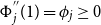$\Phi ^{''}_j(1)=\phi _j\geq 0$ . When $\phi _T=\phi _I=0$ , the model economy is equivalent to one without costly capital accumulation.

As in Jermann and Quadrini (Reference Jermann and Quadrini2012), we assume that firms use two broad categories of financing: equity and debt. Debt is preferred to equity because interest expenses are deductible (see also Hennessy and Whited (Reference Hennessy and Whited2005)). The effective gross interest rate for the firm is given by $R_t=1+r_{t}(1-\tau )$ , where $r_t$ is the interest rate on one-period intertemporal debt, $B_t$ , and $\tau$ is the tax benefit. The firm raises funds with interest-free intraperiod loans, $L_t$ , to finance working capital. This loan, which is repaied at the end of the period $t$ , is defined as

(4) \begin{equation} L_{t}=W_{t}N_{t}+I_{T,t}+I_{I,t}+B_{t}-\frac{B_{t+1}}{R_{t}}+\varphi (D_{t}), \end{equation}

where $W_{t}$ is the wage rate and $\varphi (D_{t})$ are total equity payout costs. The latter comprise the actual equity payout and equity payout adjustment costs, which account for the empirical regularity with which firm managers tend to smooth dividend payments (see, for example, Lintner (Reference Lintner1956) and Brav, et al. (Reference Brav, Graham, Harvey and Michaely2005)). The functional form for $\varphi (D_{t})$ is given by

(5) \begin{equation} \varphi (D_{t})=D_{t}+\kappa (D_t-{D})^2, \end{equation}

where the parameter $\kappa \gt 0$ determines the sensitivity of the equity payout adjustment costs to the actual equity payout, $D_t$ , and $D$ denotes the steady state level of $D_t$ . The firm’s flow of funds constraint is

(6) \begin{equation} W_{t}N_{t}+I_{T,t}+I_{I,t}+B_{t}+\varphi (D_{t})=\frac{B_{t+1}}{R_t}+Y_t. \end{equation}

Substituting equation (4) into equation (6), it is possible to verify that the intraperiod loan is equal to the firm’s production (i.e. $L_t=Y_t$ ).

Following closely Jermann and Quadrini (Reference Jermann and Quadrini2012), we assume that firms’ debt capacity is limited due to a limited enforceability of debt contracts, as firms can default on their obligations. Crucial to understand the financial contract is the assumption that the firm has all the bargaining power in the renegotiation and that the lender receives only the threat value. More specifically, it is assumed that liquidity can be easily diverted and the lender can only expropriate capital. At any time $t$ , a default may materialize after the realization of revenues but before the redemption of the intraperiod loan. At the time of default, the firm’s total liabilities are $L_t+\frac{B_{t+1}}{1+r_t}$ and the only assets available for liquidation are tangible capital and a fraction $\lambda _I$ of intangible capital. As in Jermann and Quadrini (Reference Jermann and Quadrini2012), we assume that, at the moment of contracting the loan, the liquidation value of capital is uncertain and with probability $\chi _t$ the lender is able to recover the full value of tangible capital, whereas with probability $1-\chi _t$ the lender recovers zero. When the condition occurs in which capital has a positive liquidation value, the firm offers a payment of $K_{T,t+1}+\lambda _I K_{I,t+1}-B_{t+1}/(1+r_t)$ in period $t$ and promises to pay $B_{t+1}$ tomorrow to make the lender indifferent. If capital has a liquidation value of zero, the firm does not need to make a payment in period $t$ , as the lender has no claims to settle. Based on the anticipated outcome of the renegotiation process between the firm and the lender, we derive the following borrowing constraint for the firm:Footnote ¹⁰

(7) \begin{equation} L_{t}\leq{\chi _t}\!\left (K_{T,t+1}+\lambda _I K_{I,t+1}-\frac{B_{t+1}}{1+r_{t}}\right ). \end{equation}

The parameter $\lambda _I$ , with $0\le \lambda _I\le 1$ reflects the limited collateral value of intangible capital.Footnote ¹¹ Equation (7) implies that the maximum amount of the intratemporal loan available to the firm is tied to the value of tangible capital and a limited value of intangible capital net of intertemporal debt. Hence, it is implicitly assumed that firms can also not commit to repay interperiod debt. As in Jermann and Quadrini (Reference Jermann and Quadrini2012), we conjecture that the borrowing constraint is always satisfied with equality.Footnote ¹² Using $L_t=Y_t$ , we can thus rewrite equation (7) as

(8) \begin{equation} Y_{t}={\chi _t}\!\left (K_{T,t+1}+\lambda _I K_{I,t+1}-\frac{B_{t+1}}{1+r_{t}}\right ). \end{equation}

Note that, throughout the paper, we refer to $\chi _t$ as the financial conditions variable. Similar to Jermann and Quadrini (Reference Jermann and Quadrini2012), this variable is assumed to depend on (unspecified) financial market conditions and is subject to stochastic disturbances, that is, financial shocks.

The optimization problem of the firm is to maximize the expected present value of the future equity payouts, which is given by

(9) \begin{equation} E_{t-1}\sum _{s=0}^\infty \beta ^{s}\frac{U_{C,t+s}}{U_{C,t}}(D_{t+s}), \end{equation}

where $\beta$ is the household’s discount factor, $U_{C,t}$ is the household’s marginal utility of consumption, and $E_{t-1}$ is the expectation operator conditional on information available in period $t-1$ .Footnote ¹³ The firm chooses $\{D_{t}, Y_{t}, K_{T,t+1}, K_{I,t+1}, I_{T,t}, I_{I,t}, N_t, B_{t+1}\}$ to maximize (9) subject to equations (1), (2), (6), and (8). Denoting by $\mu _t$ the multiplier for the borrowing constraint, we can summarize the first-order conditions for the firm’s optimization problem as follows:

Debt:

(10) \begin{align} 1&={\beta }{R_t}{E_{t-1}}\left (\frac{U_{C,t+1}}{U_{C,t}}\frac{\varphi^{\prime}(D_{t})}{\varphi^{\prime}(D_{t+1})}\right )+{\chi _t}{\mu _{t}}\varphi^{\prime}(D_{t})\frac{R_t}{1+r_{t}}, \end{align}

Labor:

(11) \begin{align} \frac{\partial{Y_{t}}}{\partial{N_{t}}}&=\frac{W_{t}}{1-{\mu _{t}}\varphi^{\prime}(D_{t})}, \end{align}

Tangible capital:

(12) \begin{align} Q_{T,t} &= \beta{E_{t-1}}\Bigg (\frac{U_{C,t+1}}{U_{C,t}}\frac{\varphi^{\prime}(D_{t})}{\varphi^{\prime}(D_{t+1})}\Bigg [\frac{\partial{Y_{t+1}}}{\partial{K_{T,t+1}}}\left (1-\mu _{t+1}\varphi^{\prime}(D_{t+1})\right )+Q_{T,t+1}(1-\delta _T)\Bigg ]\Bigg ) \nonumber \\ &\quad +{\chi _t}\mu _t\varphi^{\prime}(D_{t}), \end{align}

Intangible capital:

(13) \begin{align} Q_{I,t} &= \beta{E_{t-1}}\Bigg (\frac{U_{C,t+1}}{U_{C,t}}\frac{\varphi^{\prime}(D_{t})}{\varphi^{\prime}(D_{t+1})}\Bigg [\frac{\partial{Y_{t+1}}}{\partial{K_{I,t+1}}}\left (1-\mu _{t+1}\varphi^{\prime}(D_{t+1})\right )+Q_{I,t+1}(1-\delta _I)\Bigg ]\Bigg ) \nonumber \\ &\quad +{\chi _t} \lambda _I \mu _t\varphi^{\prime}(D_{t}), \end{align}

Tangible and intangible investment:

(14) \begin{align} \quad Q_{j,t}&=\frac{1-\beta{E_{t-1}}\Bigg (\frac{U_{C,t+1}}{U_{C,t}}\frac{\varphi^{\prime}(D_{t})}{\varphi^{\prime}(D_{t+1})}Q_{j,t+1}\Phi^{\prime}_j\left (\frac{I_{j,t+1}}{I_{j,t}}\right )\left (\frac{I_{j,t+1}}{I_{j,t}}\right )^2\Bigg )}{1-\Phi _j\!\left (\frac{I_{j,t}}{I_{j,t-1}}\right )-\Phi^{\prime}_j\left (\frac{I_{j,t}}{I_{j,t-1}}\right )\left (\frac{I_{j,t}}{I_{j,t-1}}\right )}, \quad \text{for}\quad j={T,I}, \end{align}

where $\frac{\partial{Y_{t}}}{\partial{N_{t}}}$ is the marginal productivity of labor, $\frac{\partial{Y_{t+1}}}{\partial{K_{T,t+1}}}$ and $\frac{\partial{Y_{t+1}}}{\partial{K_{I,t+1}}}$ are the future returns on tangible capital and intangible capital, respectively. $Q_{j,t}$ denotes the current value of type- $j$ capital, and $\varphi '(D_{t})$ is the first derivative of $\varphi (D_{t})$ with respect to $D_t$ .Footnote ¹⁴ Equation (10) is the optimally condition for intertemporal debt. It implies that a negative financial shock induces a rise in the multiplier for the borrowing constraint. Equation (11) is the optimally condition for labor demand that requires the firm to equate the marginal productivity of labor to its marginal cost. The marginal cost of labor depends negatively on $\mu _{t}$ . A higher $\mu _t$ (i.e. a tighter borrowing constraint in period $t$ ) increases the effective costs of labor and thus reduces its demand. Equations (12) and (13) are the optimally conditions for tangible capital and intangible capital, respectively. Note that the financial shock $\chi _t$ operates through opposing transmission channels in equilibrium on the value of tangible capital $Q_{T,t}$ . On the one hand, an adverse shock reduces the value of tangible capital and thus the available amount of intra-period loans. This is the direct effect of the shock to the borrowing constraint in equation (7). On the other hand, there exists an opposing indirect transmission channel operating through $\mu _t$ . Concretely, the current value of tangible capital, $Q_{T,t}$ , depends positively on $\mu _{t}$ and negatively on $\mu _{t+1}$ . The higher $\mu _{t}$ , the higher the benefit of acquiring today an additional unit of tangible capital, which allows, by relaxing the borrowing constraint, to increase the current production. Hence, when $\mu _{t}$ rises, the firm demands more tangible capital. Since intangible capital cannot be pledged as collateral in debt contracts when $\lambda _I=0$ , $\mu _t$ has no direct impact on the current value of intangible capital, $Q_{I,t}$ . Similar to tangible capital, intangible capital also depends negatively on $\mu _{t+1}$ . A higher $\mu _{t+1}$ (i.e. a tighter borrowing constraint in period $t+1$ ), decreases the current value of an additional unit of tangible capital, respectively, intangible capital, as the additional capital requires a higher working capital loan in the future. Thus, a higher $\mu _{t+1}$ reduces the demand for both tangible capital and intangible capital. Equation (14) is the Euler equation for investment in capital of type $j$ . Note that when $\phi _T=\phi _I=0$ , it follows that $Q_{T,t}=Q_{I,t}=1$ .

2.2 The representative household

The representative household maximizes its expected lifetime utility, which reads:

(15) \begin{equation} E_{t-1}\sum _{s=0}^\infty \beta ^{s}U_{t+s}(C_{t+s}, N_{t+s}), \end{equation}

where $\beta$ denotes the household’s discount factor, $C_t$ is the consumption, and $N_t$ stands for labor supply. The period utility function is defined as

(16) \begin{equation} U_t=\text{log}(C_{t}-{\epsilon }C_{t-1})+\nu \text{log}(1-N_{t}). \end{equation}

Following Smets and Wouters (Reference Smets and Wouters2003), we assume external habit formation in consumption, with $\epsilon$ measuring the influence of past economy-wide average consumption on current utility. The household’s budget constraint is

(17) \begin{equation} C_t+\frac{B_{t+1}}{1+r_t}+T_t=B_{t}+W_{t}N_{t}+D_{t}, \end{equation}

where $W_t$ denotes the wage rate, $D_t$ is the equity payout, $B_{t+1}$ stands for the new one-period intertemporal bond issued by the firm, $r_t$ is the interest rate, and 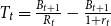$T_t=\frac{B_{t+1}}{R_t}-\frac{B_{t+1}}{1+r_t}$ is a lump-sum tax, which is equal to the firm’s tax benefit of debt.

The household chooses $\{C_t, N_t, B_{t+1}\}$ to maximize (15) subject to equation (17). The first-order conditions for the household’s optimization problem are given by

(18) \begin{align}{\beta }(1+r_{t}){E_{t-1}}\left (\frac{U_{C,{t+1}}}{U_{C,t}}\right ) &= 1, \end{align}

(19) \begin{align}U_{N,t}+U_{C,t}W_{t} &=0 \end{align}

where $U_{C,t}\equiv \frac{\partial{U_{t}}}{\partial{C_{t}}}$ is the marginal utility of consumption and $U_{N,t}\equiv \frac{\partial{U_{t}}}{\partial{N_{t}}}$ is the marginal utility of labor supply.

2.3 Discussion

In this section, we discuss the main mechanisms at work. To this end, we show in Figure 2 impulse response functions of selected model variables to a negative one standard deviation financial shock.Footnote ¹⁵ The solid lines correspond to the responses when we hold the key model parameters at their calibrated or estimated values (see Section 4), implying, most importantly, that intangible investment is much more costly to adjust than tangible investment. The dashed lines in Figure 2 correspond to the responses for an alternative setting of the investment adjustment cost parameters, where we set $\phi _T=\phi _I=0$ so that the model economy is equivalent to one without costly capital accumulation.

Figure 2.

Impulse response functions of selected model variables. Note: The figure displays impulse responses to a negative one standard deviation financial shock. The solid lines correspond to the responses when we hold the model parameters at their calibrated or estimated values, implying, most importantly, that intangible investment is much more costly to adjust than tangible investment. The dashed lines correspond to the responses of a model economy without investment adjustment costs. The marked solid lines correspond to a model economy without investment adjustment costs when we shut down the endogenous feedback of a tightening in $\mu _t$ on the value of tangible capital, $Q_{T,t}$ . Note that the dashed line and the marked solid line in the subplot for Intangible investment correspond to the scale of the y-axis on the right-hand side.

We first discuss the model-implied responses for the latter case. As is evident from the figure, a negative financial shock reduces the available amount of liabilities to finance the firm’s operations, which illustrates the direct effect of tighter financial conditions. In response, the firm reacts by reducing the equity payout. Since it is costly for the firm to change the equity payout, the firm is also forced to reduce labor. Overall, the direct effect from the borrowing constraint dominates, as output, labor, liabilities, intangible investment, and the equity payout decline. However, the indirect effect of the shock operating through an increase in the multiplier $\mu _t$ dominates on impact for the response of tangible investment. Interestingly, the firm increases tangible investment and sharply reduces intangible investment in response to the shock. The reason for this is that the tighter borrowing constraint leads the firm to reallocate resources toward pledgeable tangible capital and away from nonpledgeable intangible capital in order to mitigate the tightening of financial conditions. The firm achieves this by sharply reducing intangible investment and increasing tangible investment after the shock is realized. Hence, tangible investment and intangible investment co-move negatively in the aftermath of the financial shock.Footnote ¹⁶ This finding illustrates that the financial shock operates through two opposing transmission channels on the relative attractiveness of tangible capital. On the one hand, the direct borrowing constraint channel reduces the attractiveness of tangible investment as a marginal unit of tangible investment has a smaller relieving effect on the collateral constraint. On the other hand, the current value of tangible capital, $Q_{T,t}$ , depends positively on $\mu _t$ . The higher $\mu _t$ , the higher the benefit of acquiring today an additional unit of tangible capital, which allows, by relaxing the borrowing constraint, to increase the current production. To illustrate the quantitative importance of the direct effect from the tighter borrowing constraint for tangible investment, we shut down the multiplier channel $\mu _t$ on the value of tangible capital, $Q_{T,t}$ . To do so, we simulate the model by fixing the multiplier $\mu _t$ in equation (12) at its steady-state value to prevent that an increase in the multiplier makes tangible investment more attractive. The solid marked lines illustrate that, once the multiplier effect on the value of tangibles $Q_{T,t}$ is shut down, both types of investment decline on impact as the incentive to increase tangible investment disappears. Overall, in equilibrium, the distance between the dashed and the solid marked lines illustrates the importance of the increase of the multiplier $\mu _t$ for the case with no adjustment cost in dominating the direct effect of the borrowing constraint on impact for tangible investment.

One possible explanation for the negative co-movement between the two investment types in response to the financial shock is that it involves no cost for the firm to adjust tangible and intangible capital. The crucial role played by the presence of investment adjustment costs in the relative dynamics of tangible and intangible investment in the aftermath of a financial shock becomes evident from the solid lines in Figure 2. As can be seen, the tighter borrowing constraint forces the firm to reduce all productions inputs, which is reflected in the fall in labor as well as in tangible and intangible investment. In the presence of investment adjustment costs, it is costly for the firm to change tangible and intangible investment and, therefore, the firm is forced to cut tangible investment along with intangible investment. Intuitively, when intangible investment is much more costly to adjust than tangible investment is, the firm reduces tangible investment to a larger extent than intangible investment in order to minimize adjustment costs. Hence, the model generates a positive co-movement between tangible and intangible investment in the aftermath of the shock, with intangible investment declining much less than tangible investment.

In Figure 3, we take a closer look at the role of the relative size of the adjustment costs for tangible and intangible investment and also discuss the role of depreciation rates and the collateral value of intangible capital. To do so, we display in the figure the response of the intangible/tangible investment ratio in the left-hand side panels along with the responses of tangible and intangible investment in the right-hand side panels. The responses of tangible and intangible investment on the right correspond to the dashed-dotted lines on the left (representing the most favorable calibration of model parameters in terms of solving the co-movement problem), except in the first row where they correspond to the solid line. As the figure illustrates in the first row on the left-hand side, when tangible investment is equally costly to adjust as intangible investment is (i.e. $\phi _T = \phi _I$ = 9), the firm still reduces intangible investment by more than tangible investment so that the intangible/tangible investment ratio declines (dashed line). In this case, the firm is indifferent, in terms of minimizing adjustment costs, between reducing tangible or intangible investment. Thus, the larger decline in intangible investment than in tangible investment is due to the positive impact of the tighter borrowing constraint on the firm’s demand for tangible investment. However, at some point, when the adjustment costs for intangible investment are much higher than those for tangible investment (i.e. $\phi _T = 2, \phi _I$ = 9), the costs of reducing intangible investment to maintain tangible investment outweigh the benefits. On the one hand, the tightening of the borrowing constraint leads the firm to tilt resources toward pledgeable tangible capital at the expense of nonpledgeable intangible capital. On the other hand, the relatively high adjustment costs for intangible investment forces the firm to maintain intangible investment by reducing tangible investment. On balance, when adjustment costs for intangible investment are sufficiently larger than those for tangible investment, the firm reduces tangible investment by more than it reduces intangible investment so that the intangible/tangible investment ratio increases. The panel on the right-hand side in the first row illustrates that the impulse responses for $\phi _T=2$ and $\phi _I=9$ supports two prominent features of the data in response to a shock to the borrowing constraint. First, intangible investment is more resilient to shocks to the collateral constraint than intangible investment. Second, there is a positive co-movement between the impulses of tangibles and intangibles investment. Moreover, investment adjustment costs lead to the typical hump-shaped responses that characterizes the empirical impulse responses.

Figure 3.

Impulse response functions of the intangible/tangible investment ratio as well as tangible and intangible investment. Note: The figure displays on the left-hand side the response of the intangible/tangible investment ratio to a negative one standard deviation financial shock based on alternative settings for the investment adjustment cost parameters, the degree of collateralizability, depreciation rates and investment-to-output ratios. In the subplots in the column on the right-hand side, we show the responses for intangible and tangible investment that correspond to the dashed-dotted lines on the left, except in the first row where they correspond to the solid line.

In the model, tangible and intangible capital differ not only in terms of adjustment costs but also in terms of collateralizability, depreciation rates, and investment-to-output ratios, which we address in the following sensitivity analysis. In the panels in the second row, we set the investment adjustment costs to zero but alter the collateralizability of intangibles with $\lambda _I$ moving from no collateralbility, $\lambda _I=0$ , to full collateralizability, $\lambda _I=1$ . The right-hand panel in row two illustrates that full collateralizability solves the negative co-movement in the impulse responses of tangible and intangible investment. Nevertheless, the ratio of intangible to tangible investment falls, as shown in the panel on the left. Since the capital share of tangibles is larger than the share of intangibles, firms have an incentive to cut back more on intangible investment to cushion the tightening of financial conditions in the face of a shrinking debt capacity. However, this incentive weakens as the collateral value of intangible capital increases. Furthermore, the introduction of collateralizability into the model does not accommodate hump-shaped responses of the impulse responses of tangible and intangible investment. In the panels in the third row, we set the investment adjustment costs to zero and assume that intangible capital is not collateralizable, but let the depreciation rates move from $\delta _I=0.025$ to $\delta _I=0.1375$ . The impulse responses are shown on the right, and it can be seen that higher depreciation rates solve the co-movement problem in terms of responses of tangible and intangible investment and mitigate the decline in intangible investment. This is in line with the literature that argues that higher depreciation rates for intangibles tend to dominate the user cost of capital and make other factors, such as variations in financial conditions, relatively unimportant (see, e.g. Crouzet and Eberly (Reference Crouzet and Eberly2019)). Again, variations in the depreciation rate do not lead to hump-shaped responses and do not prevent the investment ratio (left-hand side) from falling, contrary to the data. In the panels in the last row, we illustrate the effects of increasing the intangible investment-to-output ratio from $3.4\%$ , which is the value from the national accounts data, to $6.3\%$ , which is the value for the big four euro area countries when defining intangibles in a broader sense along the lines of Corrado et al. (Reference Corrado, Haskel, Jona-Lasinio and Iommi2018). The impulse response analysis reveals that higher shares of intangible investment do not solve the co-movement problem for the range of values under consideration. The incentive to mitigate financial frictions remains the driving factor in the light of a binding collateral constraint. In sum, the results confirm our main finding within our model that when tangible and intangible investment are not costly to adjust, the intangible/tangible investment ratio falls in response to a negative financial shock.

3.1 Financial conditions

As in Jermann and Quadrini (Reference Jermann and Quadrini2012), we use the Solow residual approach to recover the series for the financial conditions variable from the model’s borrowing constraint. As shown in Section 2, the ability of the firm to borrow is affected by the variable $\chi _t$ via equation (8). Rearranging this equation and defining $B^e_{t}\equiv \frac{B_{t+1}}{1+r_t}$ as the end-of-period $t$ debt as well as $K^e_{T,t}\equiv{K_{T,t+1}}$ as the end-of-period $t$ stock of tangible capital, we can rewrite $\chi _t$ as

(20) \begin{equation} \chi _{t}=\frac{Y_{t}}{K^e_{T,t}-B^e_{t}}. \end{equation}

Log-linearizing equation (20) around the steady state, we obtain

(21) \begin{equation} \hat{\chi }_t={\chi }\frac{B^e}{Y}\hat{B}^e_{t}-{\chi }\frac{K^e_T}{Y}\hat{K}^e_{T,t}+\hat{Y}_t, \end{equation}

where the variables without a time subscript denote steady-state values and those with a hat sign represent log-deviations from steady-state values. We can use equation (21) to compute the $\hat{\chi }_t$ series once we have empirical measurements for $\hat{B}^e_{t}$ , $\hat{K}^e_{T,t}$ , and $\hat{Y}_t$ as well as appropriate values for $\chi$ , $\frac{B^e}{Y}$ and $\frac{K^e_T}{Y}$ .

To compute the series for $\hat{B}^e_{t}$ , $\hat{K}^e_{T,t}$ and $\hat{Y}_t$ , we extract the business cycle components of the empirical series for $B^e_{t}$ , $K^e_{T,t}$ and $Y_t$ , respectively.Footnote ¹⁷ For the $B^e_{t}$ , $K^e_{T,t}$ and $Y_t$ series, we use aggregated quarterly national and financial accounts data from the four largest euro area countries for the period from 1999.Q1 to 2018.Q4. The data are taken from Eurostat and ECB databases. The beginning of our sample is determined by the financial accounts data, which are available as of 1999.Q1. We construct the series for $B^e_t$ using the cumulative sum of new borrowing of non-financial corporations measured by the net flows of debt securities issued and loans received. The initial debt is set to the outstanding stock of debt securities and loans in 1999.Q1.Footnote ¹⁸ To construct the series for $K^e_{T,t}$ , we use the perpetual inventory method based on a geometric depreciation at the constant rate $\delta _T$ . Following Jermann and Quadrini (Reference Jermann and Quadrini2012), we compute the initial stock of tangible capital so that the tangible capital-to-output ratio fluctuates around a zero growth trend over the period from 1999.Q1 to 2018.Q4.Footnote ¹⁹ We assume that $\delta _T=0.025$ , which implies an annual depreciation rate of tangible capital of $10\%$ , and iterate forward using the empirical series for tangible investment, which is measured as machinery and equipment investment plus non-residential construction investment. Furthermore, we use total GDP as an empirical proxy for $Y_t$ . All data are seasonally adjusted and expressed in real terms.Footnote ²⁰ To pin down $\chi$ , $\frac{B^e}{Y}$ and $\frac{K^e_T}{Y}$ , we evaluate the model equations described in Section 2 in the steady state. After calibrating the parameters that govern the steady state of the model, we obtain $\chi =0.13$ , $\frac{B^e}{Y}=3.3$ , and $\frac{K^e_T}{Y}=11$ . Note that we provide a detailed description of the model calibration in Section 4.

Next, given the series for $\hat{B}^e_{t}$ , $\hat{K}^e_{T,t}$ , and $\hat{Y}_t$ as well as the values for $\chi$ , $\frac{B^e}{Y}$ , and $\frac{K^e_T}{Y}$ , we compute the $\hat{\chi }_t$ series. The results are shown in Figure 4. The solid line in the upper panel depicts the level series of $\hat{\chi }_t$ and the solid line in the lower panel depicts the series of the one-period changes in $\hat{\chi }_t$ . As is evident from the figure, the constructed financial conditions variable is pro-cyclical and displays pronounced fluctuations. According to our measure, borrowing conditions for firms in the euro area big four deteriorated prior to the Great Recession and tightened sharply during it. Following a temporary improvement, the measured borrowing conditions also tightened somewhat during the 2011—2013 recession, which is associated with the euro area sovereign debt crisis. Figure 4 further compares our measure to alternative indicators for proxying the degree of firms’ borrowing constraints. In the upper panel of the figure, we compare the level series of $\hat{\chi }_t$ and the credit spread index as provided by Gilchrist and Mojon (Reference Gilchrist and Mojon2018), which carefully measures the cost of market funding for non-financial firms in the four largest euro area countries a whole. For comparison purposes, the credit spread index, which is shown with dashed lines, is multiplied by $-1$ , standardized and rescaled to have the same mean and standard deviation as $\hat{\chi }_t$ . In the lower panel of the figure, we compare the series of the changes in $\hat{\chi }_t$ and the weighted average of the national diffusion indices of the change in bank credit standards for loans to non-financial corporations for the four largest euro area countries.Footnote ²¹ The bank credit standards indicator is shown by dashed lines. Note that it is multiplied by $-1$ , standardized and rescaled to have the same mean and standard deviation as the changes in $\hat{\chi }_t$ . Our financial conditions variable constructed from the theoretical model is quite good at tracking alternative measures of borrowing constraints for firms in the euro area big four. In particular, all three measures indicate a sharp deterioration in borrowing conditions during the Great Recession.

Figure 4.

Constructed financial conditions variable and alternative indicators. Note: Upper panel: The solid line depicts the level series of $\hat{\chi }_t$ . The dashed line depicts the quarterly averages of the monthly series for the credit spread index as provided by Gilchrist and Mojon (Reference Gilchrist and Mojon2018). The credit spread index is multiplied by $-1$ , standardized and rescaled to have the same mean and standard deviation as $\hat{\chi }_t$ . Lower panel: The solid line depicts the series of the one-period changes in $\hat{\chi }_t$ . The dashed line depicts the weighted average of the national diffusion indices of the net tightening of bank credit standards for loans to non-financial corporations for the four largest euro area countries. The series for the change in bank credit standards is multiplied by $-1$ , standardized and rescaled to have the same mean and standard deviation as the changes in $\hat{\chi }_t$ . The shaded areas in the upper and lower panel indicate Center for Economic Policy Research (CEPR) recession dates for the euro area as a whole.

3.2 Estimation results from the SVAR

In this section, we examine the macroeconomic effects of exogenous financial shocks. We do so by introducing the constructed financial conditions variable into a SVAR that comprises the following variables: output, household consumption, tangible investment, and intangible investment. The SVAR takes the following form:

(22) \begin{align} A \begin{bmatrix} \hat{Y}_t \\ \\[-9pt]\hat{C}_{t} \\ \\[-9pt]\hat{I}_{T,t} \\ \\[-9pt]\hat{I}_{I,t} \\ \\[-9pt]\hat{\chi }_t \end{bmatrix} = B(L) \begin{bmatrix} \hat{Y}_{t-1} \\ \\[-9pt]\hat{C}_{t-1} \\ \\[-9pt]\hat{I}_{T,t-1} \\ \\[-9pt]\hat{I}_{I,t-1} \\ \\[-9pt]\hat{\chi }_{t-1} \end{bmatrix} + u_t, \end{align}

where the factor $B(L)$ denotes a lag polynomial, with $L$ denoting the lag operator, $A$ and $B_i$ are $5\times 5$ matrices of coefficients, and $u_t$ is a mean-zero, serially uncorrelated $5\times 1$ vector of stochastic disturbances with a diagonal variance-covariance matrix. To estimate the SVAR, we use aggregated national accounts data from France, Germany, Italy, and Spain, which we obtain from Eurostat’s national accounts database. We measure output as total GDP, household consumption as final consumption of households and nonprofit institutions serving households, tangible investment as machinery and equipment investment plus nonresidential construction investment and intangible investment as investment in intellectual property products. All data are seasonally adjusted, expressed in real terms and detrended in logs using the same detrending procedure used for the construction of the $\hat{\chi }_t$ series. Following the related literature (see, e.g. Lown and Morgan (Reference Lown and Morgan2006), Gilchrist and Zakrajsek (Reference Gilchrist and Zakrajsek2012), and Walentin (Reference Walentin2014)), we identify financial shocks by applying a recursive identification scheme. That is, we assume that financial shocks affect real economy variables only with a time lag, while shocks to real economy variables impact the financial conditions variable contemporaneously. We implement these restrictions by requiring the matrix $A$ to be an unit lower triangular matrix. The SVAR is estimated over the sample from 1999.Q1 to 2018.Q4. Note that the SVAR features a constant and two lags of each variable.

Figure 5 presents the impulse response functions of all variables included in the SVAR to a negative one standard deviation financial shock. The solid lines correspond to the point estimates, and the shaded areas indicate one and two standard deviations confidence intervals, which we obtain from $2000$ bootstrap replications. As can be seen, a negative financial shock causes a significant hump-shaped reduction in the aggregate quantities as well as the constructed financial conditions variable. GDP bottoms out around $0.4$ % below trend around one year after the shock. The fall in household consumption is somewhat less pronounced in terms of amplitude than the decline in output, while the contraction in tangible investment is relatively large. The fall in intangible investment is much smaller at the peak than the decline in tangible investment. The shock also causes a gradual decline in the financial conditions variable, which bottoms out after about one year and reverts to the trend after about four years. Overall, the results suggest that financial shocks lead to economically meaningful and statistically significant declines in output, household consumption, and the two investment aggregates. Importantly, tangible and intangible investment co-move positively in response to the financial shock, with intangible investment declining much less than tangible investment. Note that these results are robust to the specification of additional lags, the use of alternative detrending methods and the introduction of additional variables.Footnote ²² In addition, these results are in line with what Bianchi et al. (Reference Bianchi, Kung and Morales2019) find for the US. In particular, they report that intangible investment roughly drops by only half as much as tangible investment does in response to a debt financing shock.

Figure 5.

SVAR- and model-based impulse response functions. Note: The figure displays SVAR- and model-based impulse responses to a negative one standard deviation financial shock. The solid lines are SVAR-based impulse responses and the dashed lines are model-based impulse responses (see Section (4)). The shaded areas denote the one and two standard-deviations confidence intervals around the SVAR-based estimates based on $2{,}000$ bootstrap replications.

Table 1 depicts the amount of variation in the variables included in the SVAR explained by the identified financial shock. The financial shock accounts for a significant fraction of the variation in output, household consumption, tangible investment, and intangible investment. The finding that the financial shock is an important source of variation in intangible investment is consistent with the view that the collateral constraint implies quantitatively important spill over effects from tangible to intangible investment. For the US, Bianchi et al. (Reference Bianchi, Kung and Morales2019) argue that debt financing shocks are more important for variations in tangible investment compared to intangible investment. The structural differences between euro area and US debt and equity markets may be responsible for the divergent outcomes. Interestingly, we find that up to around 60% of the variation in the constructed financial conditions variable is due to the financial shock itself. Hence, a large part of the variation in the constructed financial conditions series is not due to exogenous shifts but, rather, reflects other shocks.

Table 1.

Percentage variance due to financial shocks

Note: The table displays SVAR-based variance decompositions from a one standard deviation financial shock. The numbers in square brackets denote the boundaries of the associated 95% confidence interval.

4.1 Calibrated model parameters and driving process for the financial conditions variable

Table 2 provides an overview of the calibrated model parameters. These parameters pertain to the steady-state values of observable variables in the model and can therefore be set with steady-state targets.Footnote ²⁴ We set $\beta =0.995$ , which implies a steady-state annual real interest rate of $2\%$ . The labor disutility parameter, $\nu$ , is set in such a way that the steady-state labor supply is equal to $0.3$ .Footnote ²⁵ We choose the intangible capital income share parameter, $\alpha _{K_I}$ , to have a steady state share of intangible investment in output of $\frac{I_I}{Y}=0.035$ , which is equal to the observed average share of investment in intellectual property products in total GDP for the euro area big four for the period from 1999.Q1 to 2018.Q4. The tangible capital income share parameter, $\alpha _{K_T}$ , is set so as to have a steady state share of labor income in output of $\frac{WN}{Y}=0.64$ . The tax wedge, $\tau$ , is set to $0.3$ . The depreciation rate of tangible capital, $\delta _T$ , is $0.025$ . As for the depreciation rate of intangible capital, $\delta _I$ , we set $\delta _I=0.05$ , which implies an annual depreciation rate of $20\%$ . This magnitude of $\delta _I$ reflects the assumption that intangible assets depreciate faster overall than tangible assets and roughly matches the unweighted average of the annual depreciation rates of R&D ( $15\%$ ), mineral exploration ( $7.5\%$ ), and computer software and databases ( $32\%$ ) as provided in Corrado et al. (Reference Corrado, Haskel, Jona-Lasinio and Iommi2018). We set the steady-state value of $\chi _t$ to have the steady-state end-of-period debt-to-output ratio equal to $\frac{B^e}{Y}=3.3$ , which matches the observed average ratio of the end-of-period debt of nonfinancial corporations over total GDP for the four largest economies of the euro area as a whole for the period from 1999.Q1 to 2018.Q4. Given the values for $\chi$ , $\beta$ , $\frac{{W}{N}}{Y}$ , $\frac{I_I}{Y}$ , $\tau$ , $\delta _T$ , $\delta _I$ , and $\frac{B^e}{Y}$ , the steady-state end-of-period tangible capital-to-output ratio is $\frac{K^e_T}{Y}=11$ . Turning to the assumed driving process for the financial conditions variable, we consider a process with feedback effects from other variables, as in the empirical model. More specifically, we assume that the driving process for $\hat{\chi }_t$ in the theoretical model is identical to the last equation of the SVAR system, which reads:Footnote ²⁶

(23) \begin{align} A^5 \begin{bmatrix} \hat{Y}_t \\ \hat{C}_{t} \\ \hat{I}_{T,t} \\ \hat{I}_{I,t} \\ \hat{\chi }_t \end{bmatrix} = B_0^5 \begin{bmatrix} \hat{Y}_{t-1} \\ \hat{C}_{t-1} \\ \hat{I}_{T,t-1} \\ \hat{I}_{I,t-1} \\ \hat{\chi }_{t-1} \end{bmatrix} + B_1^5 \begin{bmatrix} \hat{Y}_{t-2} \\ \hat{C}_{t-2} \\ \hat{I}_{T,t-2} \\ \hat{I}_{I,t-2} \\ \hat{\chi }_{t-2} \end{bmatrix}+ u_{{\chi },t}, \end{align}

where $A^5$ , $B^5_0$ , and $B^5_1$ are $5\times 1$ row vectors of coefficients that correspond to the 5th row of the matrices $A$ , $B_0$ , and $B_1$ , respectively, and $u_{{\chi },t}$ is the financial shock. Note that this implies that the theoretical model includes the same feedback effects between the financial conditions variable and the real economy variables as given in the SVAR. However, the dynamic behavior of the real economy variables is dictated by the mechanisms embedded in the theoretical model. As a result, the theoretical and the empirical responses of the financial conditions variable to a financial shock are not necessarily identical (see also Ravn et al. (Reference Ravn, Schmitt-Grohe and Uribe2012)). The standard deviation of the financial shock, which is also obtained from the SVAR, is set to $\sigma _{u_{\chi }}=0.0014$ .

Table 2.

Calibrated model parameters

4.2 Prior and posterior distributions

In the upper half of Table 3, we present the prior distributions of the estimated parameters. We assume that the habit formation parameter, $\epsilon$ , follows a beta distribution. We choose a prior mean of $0.7$ and a standard deviation equal to $0.1$ . The equity payout cost parameter, $\kappa$ , is assumed to follow an inverse gamma distribution and is centered at $0.2$ , as in Jermann and Quadrini (Reference Jermann and Quadrini2012). The prior probabilities of the investment adjustment cost parameters, $\phi _T$ and $\phi _I$ , are gamma distributions. We set the prior means to $4$ and the standard deviations to $2$ . Hence, we do not force intangible investment to be more persistent than tangible investment and allow for a large parameter domain.

Table 3.

Prior and posterior distributions of model parameters

Note: Posterior distributions of model parameters are obtained using the Metropolis-Hastings algorithm with 500,000 draws and a burn-in of 25%. The acceptance rate is 30%.

The lower half of Table 3 reports the posterior mode, mean, and 95% probability intervals for the estimated parameters. We obtain a posterior mean of $0.87$ for the habit formation parameter, implying that household consumption adjusts very slowly to financial shocks. The posterior mean of $\kappa$ is $0.6$ . This value is larger than the value for the US as estimated in Jermann and Quadrini (Reference Jermann and Quadrini2012). Turning to the investment adjustment cost parameters, we find that the posterior estimates of $\phi _T$ and $\phi _I$ are significantly different from zero, confirming that investment adjustment costs are an important feature of the model for capturing the empirical persistence of both tangible and intangible investment. Interestingly, the posterior mean of the adjustment cost parameter for intangible investment is much higher than that for tangible investment, even though we set the same prior means. Specifically, the posterior mean of $\phi _I$ implies an estimate of the elasticity of intangible investment with respect to a 1% temporary increase in the current price of installed intangible capital of $0.1$ . The corresponding elasticity for tangible investment is found to be $0.5$ . These elasticities are close to those implied by the estimates for the US reported in Bianchi et al. (Reference Bianchi, Kung and Morales2019), who use R&D investment from the national accounts to proxy intangible investment. The finding that intangible investment adjusts much more slowly to its costs than is the case for tangible investment is also fully in accord with what is obtained in the finance literature, as found in Peters and Taylor (Reference Peters and Taylor2017). In addition, the finding is in line with the estimates presented in Chiavari and Sampreet (Reference Chiavari and Sampreet2021), who report higher adjustment costs for intangibles compared to tangible investment. In the literature, many argue that intangible capital (in particular R&D capital) has high adjustment costs and possibly much higher adjustment costs than tangible capital (see, e.g. Himmelberg and Petersen (Reference Himmelberg and Petersen1994), Hall (Reference Hall2002) and Brown et al. (Reference Brown, Fazzari and Petersen2009)), because adjusting intangible capital typically involves adjusting the number of highly educated employees, who have high searching, training or replacement costs. Our estimation results are consistent with this view. Overall, we find that the priors and posteriors are quite different, suggesting that the data are informative about the model’s parameters. Given the relatively large posterior estimates for the habit formation parameter, $\epsilon$ , and the equity payout costs parameter, $\kappa$ , we have performed a sensitivity analysis with respect to these parameters. We found that the posterior estimates for the investment adjustment cost parameters, $\phi _T$ and $\phi _I$ , are not particularly sensitive to lower values of $\epsilon$ and $\kappa$ .

4.3 Model-implied impulse response functions

Figure 5 depicts with dashed lines the model-implied impulse response functions of output, household consumption, tangible investment, intangible investment, and the constructed financial conditions variable to a negative one standard deviation financial shock. As can be seen from the figure, the theoretical model does well at reproducing the observed transmission of financial shocks based on the SVAR results. The model accounts for the hump-shaped reduction in the real economic quantities as well as the constructed financial conditions variable. Most of the model responses are close to the point estimates from the SVAR; and almost all model responses lie within the one standard deviation confidence intervals around the SVAR-based estimates. Importantly, the model predicts a strong fall in tangible investment and a relatively small decline in intangible investment. As explained above, this positive co-movement between tangible and intangible investment as well as the relative resilience of intangible investment poses a challenge for a model without costly capital accumulation.