1 Introduction
The overall structure and dynamics of premixed flames are strongly altered by the presence of turbulence, particularly at high intensities, giving rise to a wealth of complicated phenomena such as front corrugations, unsteady flame stretch, chaotic pulsations, flame broadening and broken reaction layers. Characteristic regime diagrams, for instance, are attempts to estimate these changes in terms of global non-dimensional parameters such as the Reynolds, Karlovitz and Damköhler numbers (Peters Reference Peters2000), but such approaches provide only order-of-magnitude descriptions of how turbulence and flames interact. In contrast, effects of premixed flames on turbulence in the surrounding gas have traditionally received much less attention.
Thermal expansion from chemical reactions leads to hydrodynamic coupling with the ambient turbulence in a complex manner that is difficult to quantify, partly because of the challenge associated with conceptualizing turbulence physics far from the homogeneous, isotropic and solenoidal conditions that dominate classic turbulence theories (Batchelor Reference Batchelor1959). In turbulent premixed combustion, depending on the characteristic regime associated with the prevailing values of the non-dimensional parameters of the configuration, the spatial scales at which the chemical heat is released may range from the inertial subrange to thin layers embedded in Kolmogorov eddies.
Theoretical analyses of multi-scale interactions in turbulent premixed flames become rapidly intractable due to several factors, including complex chemical-kinetic and transport effects, the associated challenges of performing Fourier spectral analyses in such strongly inhomogeneous and anisotropic flows, and complications due to order-unity density variations. One relevant theoretical analysis of this type was made by Aldredge & Williams (Reference Aldredge and Williams1991) for single-step chemical kinetics in a transverse-periodic configuration similar to the one treated computationally in this study (i.e. see figure 1 and § 2 for details), but it was limited to weak turbulence passing through a thin flame, as in the wrinkled-flamelet regime. In that limit, the turbulence intensity is small and the eddy turnover time is much larger than the flame-transit time. As a consequence, to first order, the problem admits a linearized solution that describes the rapid straining of eddies as they pass across the thin flame, with the nonlinear convective dynamics required for inter-scale energy transfer and combustion-induced backscatter becoming higher-order effects that are not essential to the interaction (O’Brien et al. Reference O’Brien, Towery, Hamlington, Ihme, Poludnenko and Urzay2017). More recently, Fourier-based computational analyses of energy transfer in flames subjected to stronger turbulent intensities have also rendered useful information about the scales participating in energy fluxes, including backscatter (Kolla et al. Reference Kolla, Hawkes, Kerstein, Swaminathan and Chen2014; Towery et al. Reference Towery, Poludnenko, Urzay, O’Brien, Ihme and Hamlington2016).
In most configurations, Fourier analyses of turbulent premixed flames require transformation into spectral space of the flow variables along homogeneous planes parallel to the mean flame front. However, because of the instantaneous corrugations of the flame, both unburnt and burnt gases tend to simultaneously be captured in the Fourier-transformed fields and therefore both participate in the overall spectral dynamics across the front with individual contributions that cannot be easily separated. Given the instantaneous spatial localization of the chemical heat release, perhaps a more convenient approach is to analyse multi-scale interactions at specific locations within the flame, as characterized, for instance, by the local instantaneous value of a progress variable.
An increased degree of spatial localization of the spectral dynamics is enabled by the wavelet transform (Grossmann & Morlet Reference Grossmann and Morlet1984; Mallat Reference Mallat1989, Reference Mallat2008), which has been used previously as a diagnostic tool to characterize structural aspects of incompressible turbulent flows (Meneveau Reference Meneveau1991; Farge Reference Farge1992; Brasseur & Wang Reference Brasseur and Wang1995; Dunn & Morrison Reference Dunn and Morrison2003; Ruppert-Felsot, Farge & Petitjeans Reference Ruppert-Felsot, Farge and Petitjeans2009; Schneider & Vasilyev Reference Schneider and Vasilyev2010; Bassenne et al. Reference Bassenne, Urzay, Schneider and Moin2017; Urzay, Doostmohammadi & Yeomans Reference Urzay, Doostmohammadi and Yeomans2017). However, although concepts exist for using wavelets to numerically solve chemically reacting flows by exploiting their automatic grid adaptation and compression capabilities (Bockhorn, Froölich & Schneider Reference Bockhorn, Froölich and Schneider1999; Prosser & Cant Reference Prosser and Cant2011; Jones & Lichtl Reference Jones and Lichtl2015), they appear to have never been deployed for the fundamental task of investigating multi-scale transfer of energy in turbulent flames, the latter representing the central subject of this study.
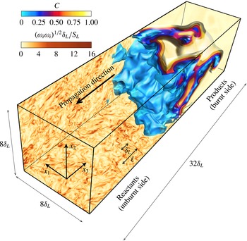
Instantaneous DNS snapshot of the flow field for the case parameters described in table 1, including progress-variable
 $C$
isosurfaces near the front along with contours of the vorticity magnitude
 $(\unicode[STIX]{x1D714}_{i}\unicode[STIX]{x1D714}_{i})^{1/2}$
. The streamwise length of the visualization domain shown here is one quarter of the full computational domain. The symbols
 $\unicode[STIX]{x1D6FF}_{L}$
and
 $\ell$
correspond to the laminar flame thickness and integral length respectively.

In this investigation, a three-dimensional (3D) discrete wavelet multi-resolution analysis of direct numerical simulations (DNS) of a turbulent premixed flame is performed, with a focus on quantifying the transfer of kinetic energy across scales. The computational set-up involves a premixed flame propagating in forced homogeneous–isotropic turbulence along an unconfined domain with periodic boundary conditions on the transverse directions, as shown in figure 1. A Cartesian coordinate system
 $\{x_{1},x_{2},x_{3}\}$
is defined in which
 $x_{3}$
is aligned with the streamwise direction pointing towards the products. The discrete wavelet multi-resolution algorithm by Mallat (Reference Mallat1989) is employed to wavelet-transform the numerical results. A spectral analysis is performed based on extending the wavelet-based energetics formulation for incompressible flows in Meneveau (Reference Meneveau1991) to chemically reacting compressible flows. Besides examining the energy spectra, an analysis of inter-scale and subfilter-scale (SFS) cumulative energy fluxes is performed, including the calculation of statistics of those quantities conditioned on the local instantaneous progress variable. In particular, the inter-scale flux describes the rate at which energy is injected or drained from a given scale at a given spatial location. Conversely, the SFS-cumulative flux corresponds to the overall transfer of energy crossing a given scale cutoff at a given region of space, with all smaller scales embedded in that region being used for the computation of the transfer rate. In the results, the focus is on energy fluxes related to the convection and pressure-gradient mechanisms of momentum transport because of their relevance for subgrid-scale energetics in turbulent premixed flames (O’Brien et al.
Reference O’Brien, Towery, Hamlington, Ihme, Poludnenko and Urzay2017).
The remainder of this paper is organized as follows. The DNS computational set-up is characterized in § 2. The wavelet multi-resolution framework is summarized in § 3. A formulation to examine energy transfer in wavelet space for compressible turbulent flows is provided in § 4. Unconditioned statistics for energy spectra and inter-scale fluxes are described in § 5. A method for conditioning the statistics on the local instantaneous progress variable is introduced in § 6. Using this method, progress-variable-conditioned statistics are provided in § 7 for energy spectra and inter-scale fluxes, and in § 8 for the SFS-cumulative fluxes. Lastly, conclusions are provided in § 9. Four appendices are included which contain supplementary definitions for the wavelet formulation (appendix A), describe the boundary conditions employed in the wavelet transform (appendix B), provide a formulation of large-scale energy fluxes (appendix C) and illustrate the collapse of the wavelet energetics formulation on well-known energy balance equations for compressible turbulent flows in triply periodic domains (appendix D).
The main emphasis of this study is on turbulent premixed combustion. However, it is worth mentioning that the resulting formulation of the energetics in wavelet space is also applicable for the analysis of multi-scale energy transfer in other variable-density flows unrelated to combustion. These include, for instance, general compressible turbulent flows, such as shock–turbulence interactions, or two-phase turbulent flows where each phase is incompressible but they have different densities.
2 Computational set-up
The formulation of the problem solved here is described elsewhere (Towery et al.
Reference Towery, Poludnenko, Urzay, O’Brien, Ihme and Hamlington2016; O’Brien et al.
Reference O’Brien, Towery, Hamlington, Ihme, Poludnenko and Urzay2017). In short, the numerical code is the finite-volume one described in Poludnenko & Oran (Reference Poludnenko and Oran2010) and integrates the unsteady compressible chemically reacting Navier–Stokes conservation equations for mass, momentum, species and total energy for a mixture of perfect gases. The dynamic viscosity, thermal conductivity and mass diffusivity follow temperature power laws with exponent 0.7. The chemical-kinetic description consists of a single-step irreversible Arrhenius reaction where the reactant mass fraction is denoted as
 $Y$
. In the following, however, use of the progress variable
 $C=1-Y$
is made, with
 $C=0$
on the reactant side and
 $C=1$
on the product side.
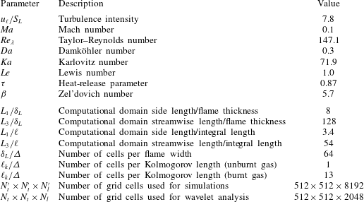
The physical and computational parameters of the simulations are summarized in table 1. In the notation, the turbulence intensity
 $u_{\ell }/S_{L}$
, Karlovitz number
 $Ka=t_{L}/t_{k}$
and Taylor–Reynolds number
 $Re_{\unicode[STIX]{x1D706}}=u_{\ell }\unicode[STIX]{x1D706}/\unicode[STIX]{x1D708}_{u}$
, are based on the integral velocity
 $u_{\ell }$
, the laminar flame speed
 $S_{L}$
, the Taylor scale
 $\unicode[STIX]{x1D706}$
and the flame-transit time
 $t_{L}=\unicode[STIX]{x1D6FF}_{L}/S_{L}$
, where
 $\unicode[STIX]{x1D6FF}_{L}$
is the laminar flame thickness, and
 $t_{k}$
and
 $\unicode[STIX]{x1D708}_{u}$
are the Kolmogorov time and kinematic viscosity on the reactant side respectively.
Physical (top) and computational (bottom) parameters of the simulations.

The computations are carried out on a uniform Cartesian grid of
 $N_{t}^{\prime }\times N_{t}^{\prime }\times N_{l}^{\prime }=512\times 512\times 8192$
elements in the
 $x_{1}$
,
 $x_{2}$
and
 $x_{3}$
directions respectively (see figure 1 for axis orientation). In this notation,
 $N_{t}^{\prime }$
and
 $N_{l}^{\prime }$
refer to the numbers of elements of the simulation grids in the spanwise and streamwise directions respectively. For the wavelet analysis described below, a portion of the simulation grid is used that is smaller in the streamwise direction and contains
 $N_{t}\times N_{t}\times N_{l}=512\times 512\times 2048$
elements, where the absence of primes in the notation distinguishes these numbers of elements from those used in the simulations. The wavelet-analysis grids move with the flame in such a way that they are centred around the streamwise location where the instantaneous spanwise-averaged progress variable reaches
 $C=0.5$
. In addition, their boundaries are always located at least
 $1000$
grid points away from the true simulation boundaries in the
 $x_{3}$
direction. The number of grid points of these shortened grids in the streamwise direction,
 $N_{l}=2048$
, ensures that the spanwise-averaged progress variable ranges at least from
 $C=0.005$
to
 $0.995$
within the domain dedicated to the wavelet analysis.
The width of the computational domain used for the simulations is
 $L_{1}/\unicode[STIX]{x1D6FF}_{L}=L_{2}/\unicode[STIX]{x1D6FF}_{L}=8$
, while its length is
 $L_{3}/\unicode[STIX]{x1D6FF}_{L}=128$
. This grid resolution provides
 $3.4$
and
 $54$
integral lengths in the spanwise and streamwise directions respectively. The minimum grid spacing
 $\unicode[STIX]{x1D6E5}$
is comparable to the Kolmogorov length on the reactant side,
 $\ell _{k}/\unicode[STIX]{x1D6E5}=1$
. In the burnt gases, the effective resolution increases as a result of the increase in kinematic viscosity with temperature, which yields
 $\ell _{k}/\unicode[STIX]{x1D6E5}=13$
there. Additionally, the flame thickness is resolved with 64 grid points across.
The boundary conditions in the
 $x_{1}$
and
 $x_{2}$
directions are periodic. The boundaries in the
 $x_{3}$
direction are periodic prior to the establishment of the premixed flame. Extrapolation boundary conditions are used thereafter, in which the variables in the cell adjacent to the boundary are copied into the four ghost cells beyond the boundary. In practice, this allows gases to flow into and out of the domain without causing a build-up of pressure (Poludnenko Reference Poludnenko2015).
The simulations are initialized as follows. First, in the absence of combustion, forced turbulence is allowed to develop everywhere in the computational domain for a duration of
 $6t_{\ell }$
, where
 $t_{\ell }=\ell /u_{\ell }$
is the integral time. After the initial transient, a planar laminar flame is inserted in the simulation domain and is allowed to develop for another
 $6t_{\ell }$
, during which transition to a fully turbulent reacting regime occurs, with 15 three-dimensional solution snapshots recorded thereafter during a time interval of approximately
 $3t_{\ell }$
. All spectral statistics shown below are ensemble-averaged over this sampling time interval, during which the solutions are relatively stationary. The turbulence is sustained through a solenoidal isotropic forcing term in the momentum equation that remains active for the remainder of the simulations. This term only acts upon the largest scales and its details can be found elsewhere (Poludnenko & Oran Reference Poludnenko and Oran2010). It should be noted that the kinetic energy of unforced turbulence would have otherwise decayed by a factor of order unity after approximately one flame-transit time, as prescribed by the relatively low Damköhler number
 $Da=t_{\ell }/t_{L}=0.3$
employed here.
In table 1, additional parameters participating in the simulations are the unity Lewis number of the reactant
 $Le=D_{T,u}/D_{F,u}$
based on the thermal
 $D_{T,u}$
and mass
 $D_{F,u}$
diffusivities on the unburnt side, the Mach number
 $Ma=S_{L}/a_{u}$
based on the speed of sound on the reactant side
 $a_{u}$
, the heat-release parameter
 $\unicode[STIX]{x1D70F}=(T_{b}-T_{u})/T_{b}$
based on the temperatures on the burnt
 $T_{b}$
and unburnt
 $T_{u}$
sides of the flame, and the Zel’dovich number
 $\unicode[STIX]{x1D6FD}=\unicode[STIX]{x1D70F}T_{a}/T_{b}$
based on the activation temperature
 $T_{a}$
. The value of the heat-release parameter
 $\unicode[STIX]{x1D70F}$
indicates that the temperature increases by a factor of approximately 7, which leads to a
 $28$
-fold increase in the kinematic viscosity on the burnt side of the flame. In addition, the Mach number is necessarily a small parameter in premixed flame propagation, as required by the many molecular collisions needed to release chemical heat, while
 $\unicode[STIX]{x1D6FD}$
is a moderately large parameter, as typically occurs in combustion processes which tend to involve exothermic chemical reactions with large energy barriers.
The numerical integrations based on the aforementioned computational set-up yield the flow fields shown in figure 1 for the set of characteristic parameters given in table 1. In the visualizations, it is important to notice that the flame thickness
 $\unicode[STIX]{x1D6FF}_{L}=0.42\ell$
is located at intermediate eddy scales that could be associated with an inertial subrange. In principle, the resulting combustion regime corresponds to the thin-reaction zones (Peters Reference Peters2000), although the simulation results do not show significant flame broadening.
The flow field upstream of the flame is characterized in figure 1 by the contours of the vorticity magnitude, showing a wide range of eddy scales. As the flame propagates into the upstream turbulence, it becomes highly corrugated across wavelengths that span from the integral length
 $\ell$
to smaller lengths observed on the cold edge of the preheat zone. The flame front ceases to be a well-defined one to become a highly contorted structure that simultaneously extends up to long distances upstream and downstream from its mean streamwise position, including long tongues of reactant penetrating far downstream. Detailed analyses of turbulent-flame dynamics in similar configurations are available elsewhere (Poludnenko & Oran Reference Poludnenko and Oran2010; Hamlington, Poludnenko & Oran Reference Hamlington, Poludnenko and Oran2011).
In the context of the Fourier analyses discussed in § 1, the large departures from a planar front found in these simulations lead to conceptual difficulties in deploying Fourier transforms along spanwise planes to study energy-transfer dynamics, since the front becomes highly delocalized in the streamwise coordinate. As a result, each
 $x_{3}$
slice tends to be well populated with both burnt and unburnt gases. Conversely, wavelet methods circumvent this problem, with some limitations, by enabling the localization of the spectral analysis along the contorted front, as shown below.
3 Wavelet formulation
Consider a general 3D scalar field
 $y$
(e.g. the progress variable
 $C$
or one component of the velocity
 $u_{i}$
or vorticity
 $\unicode[STIX]{x1D714}_{i}$
), described in physical space by its pointwise values at cell-centre locations
 $$\begin{eqnarray}\boldsymbol{x}_{\mathbf{0}}=(i\unicode[STIX]{x1D6E5},j\unicode[STIX]{x1D6E5},k\unicode[STIX]{x1D6E5})\end{eqnarray}$$
of the primitive grid
 $N_{t}\times N_{t}\times N_{l}$
used for the wavelet analysis, which corresponds to a subset of the DNS grid that has the same resolution
 $\unicode[STIX]{x1D6E5}$
as described in § 2 and where
 $i=1/2,3/2,\ldots ,N_{t}-1/2$
,
 $j=1/2,3/2,\ldots ,N_{t}-1/2$
and
 $k=1/2,3/2,\ldots ,N_{l}-1/2$
are the spatial index positions. The dependence of
 $y$
on time
 $t$
will be omitted for brevity. The expansion of
 $y$
in a fully discrete 3D wavelet series is

The discrete wavelet representation (3.2) is a particular choice for the notation that is convenient here because of the numerical data emerging from the simulations. Alternative representations, including formally equivalent semi-discrete wavelet formulations, could have also been employed without any loss of generality by performing minimal modifications of the notation. In this formulation,
 ${\mathcal{G}}^{(s,d)}[\boldsymbol{x}_{\mathbf{0}}-\boldsymbol{x}_{\boldsymbol{s}}]$
and
 ${\mathcal{H}}^{({\mathcal{S}})}[\boldsymbol{x}_{\mathbf{0}}-\boldsymbol{x}_{\boldsymbol{{\mathcal{S}}}}]$
are 3D multiplicative combinations of the one-dimensional (1D) discrete orthonormal wavelet basis and scaling functions. The wavelets are collocated at a given scale
 $s$
in scale-dependent grids denoted by
 $\boldsymbol{x}_{\boldsymbol{s}}=2^{s-1}(i\unicode[STIX]{x1D6E5},j\unicode[STIX]{x1D6E5},k\unicode[STIX]{x1D6E5})$
. These are grids of size
 $N_{s}=N_{t}/2^{s}\times N_{t}/2^{s}\times N_{l}/2^{s}$
, with
 $i=1,3,5,\ldots ,N_{t}/2^{s-1}-1$
,
 $j=1,3,5,\ldots ,N_{t}/2^{s-1}-1$
and
 $k=1,3,5,\ldots ,N_{l}/2^{s-1}-1$
. Additionally,
 $d=(1,2,\ldots ,7)$
is a wavelet-directionality index and
 $s=(1,2,\ldots ,{\mathcal{S}})$
are scale exponents, with
 ${\mathcal{S}}=\log _{2}N_{t}=9$
the maximum number of resolution levels allowed by the grid in these simulations. In the present configuration,
 $\boldsymbol{x}_{\mathbf{1}}$
is a grid of
 $256\times 256\times 1024\simeq 67\,000\,000$
elements, while
 $\boldsymbol{x}_{\boldsymbol{{\mathcal{S}}}}$
has
 $1\times 1\times 4=4$
elements. A simpler example of the wavelet-collocation grids
 $\boldsymbol{x}_{\boldsymbol{s}}$
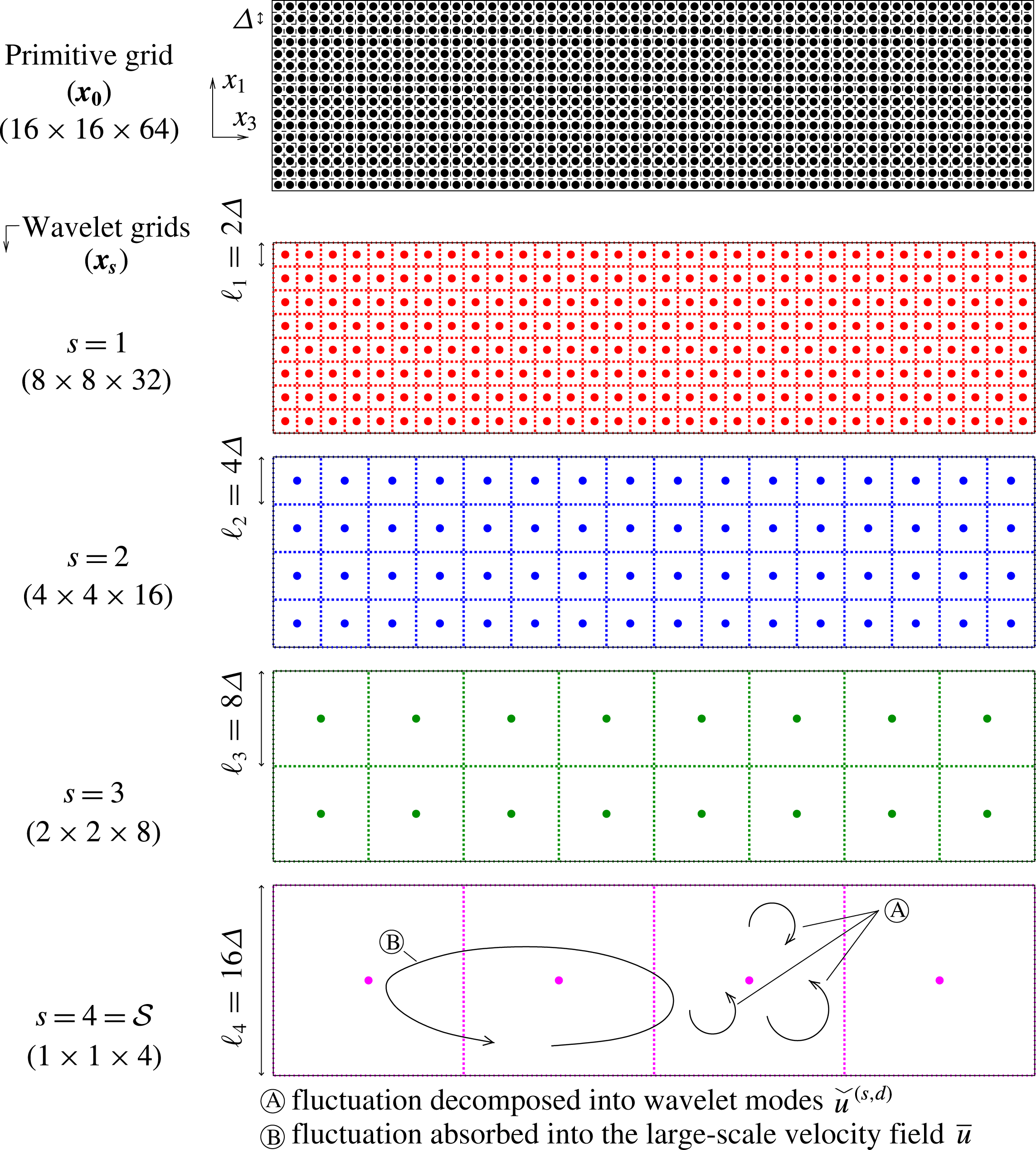
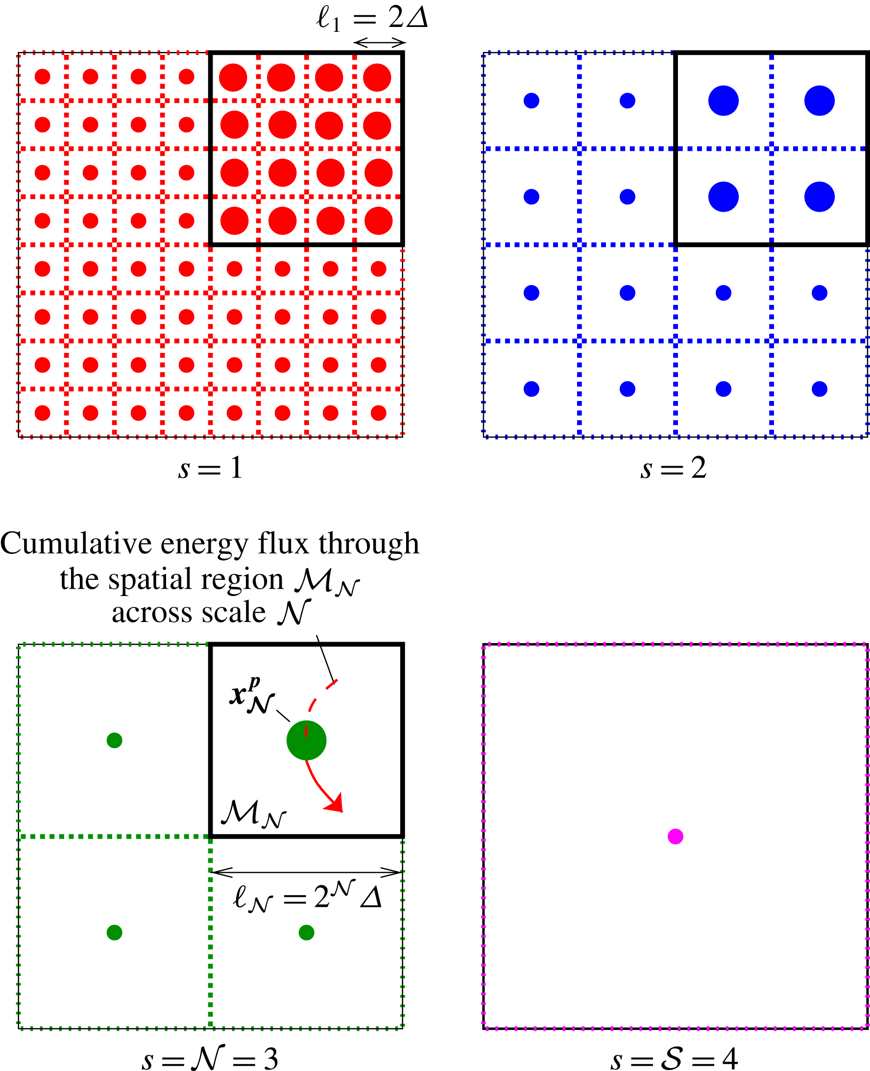
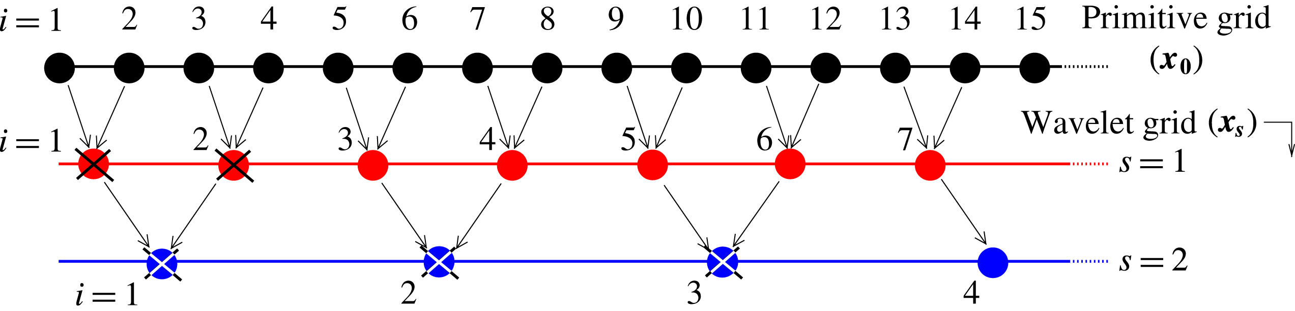
resulting from the wavelet multi-resolution framework is provided in figure 2 for a coarser grid that nonetheless has the same aspect ratio as the one used in these simulations. For completeness, basic relations between discrete wavelet representations and the more traditional continuous ones, including definitions of
 ${\mathcal{G}}^{(s,d)}[\boldsymbol{x}_{\mathbf{0}}-\boldsymbol{x}_{\boldsymbol{s}}]$
and
 ${\mathcal{H}}^{({\mathcal{S}})}[\boldsymbol{x}_{\mathbf{0}}-\boldsymbol{x}_{\boldsymbol{{\mathcal{S}}}}]$
along with derivations of relevant orthonormality conditions, are provided in appendix A.
Lateral view of wavelet-collocation grids
 $\boldsymbol{x}_{\boldsymbol{s}}$
for each decomposition level
 $s$
in the wavelet multi-resolution framework, illustrated for a simpler primitive grid
 $\boldsymbol{x}_{\mathbf{0}}$
of
 $N_{t}\times N_{t}\times N_{l}=16\times 16\times 64$
elements in the
 $x_{1}$
,
 $x_{2}$
and
 $x_{3}$
directions respectively. The maximum wavelet-decomposition level allowed by the grid in this example is
 ${\mathcal{S}}=\log _{2}16=4$
. Schematics of fluctuations A (of size smaller than or equal to
 $\ell _{{\mathcal{S}}}$
and that can be decomposed into wavelets) and B (of size larger than
 $\ell _{{\mathcal{S}}}$
and that are absorbed into the large-scale field) are sketched in the bottom panel.

In (3.2), the symbol
 $\check{y}^{(s,d)}$
represents a set of
 $(N_{t}^{3}-1)N_{l}/N_{t}\simeq 537\,000\,000$
wavelet coefficients, whose expression is obtained by multiplying (3.2) by
 ${\mathcal{G}}^{(s^{\prime },d^{\prime })}[\boldsymbol{x}_{\mathbf{0}}-\boldsymbol{x}_{\boldsymbol{s}^{\prime }}]$
, summing over
 $\boldsymbol{x}_{\mathbf{0}}$
and making use of the following orthonormality conditions in the discrete wavelet representation:
 $$\begin{eqnarray}\mathop{\sum }_{\boldsymbol{x}_{\mathbf{0}}}{\mathcal{G}}^{(s,d)}[\boldsymbol{x}_{\boldsymbol{ 0}}-\boldsymbol{x}_{\boldsymbol{s}}]{\mathcal{G}}^{(s^{\prime },d^{\prime })}[\boldsymbol{x}_{\mathbf{0}}-\boldsymbol{x}_{\boldsymbol{s}^{\prime }}]=\unicode[STIX]{x1D6FF}_{s,s^{\prime }}\unicode[STIX]{x1D6FF}_{d,d^{\prime }}\unicode[STIX]{x1D6FF}_{\boldsymbol{x}_{\boldsymbol{s}},\boldsymbol{x}_{\boldsymbol{s}^{\prime }}}\end{eqnarray}$$
and
 $$\begin{eqnarray}\mathop{\sum }_{\boldsymbol{x}_{\mathbf{0}}}{\mathcal{G}}^{(s,d)}[\boldsymbol{x}_{\boldsymbol{ 0}}-\boldsymbol{x}_{\boldsymbol{s}}]{\mathcal{H}}^{({\mathcal{S}})}[\boldsymbol{x}_{\boldsymbol{ 0}}-\boldsymbol{x}_{\boldsymbol{{\mathcal{S}}}}]=0,\end{eqnarray}$$
which yield
 $$\begin{eqnarray}\check{y}^{(s,d)}[\boldsymbol{x}_{\boldsymbol{ s}}]=\mathop{\sum }_{\boldsymbol{x}_{\mathbf{0}}}y[\boldsymbol{x}_{\mathbf{0}}]{\mathcal{G}}^{(s,d)}[\boldsymbol{x}_{\boldsymbol{ 0}}-\boldsymbol{x}_{\boldsymbol{s}}],\end{eqnarray}$$
where
 $\unicode[STIX]{x1D6FF}_{ij}$
is the Kronecker delta. In this study, the orthonormal basis functions
 ${\mathcal{G}}^{(s,d)}[\boldsymbol{x}_{\mathbf{0}}-\boldsymbol{x}_{\boldsymbol{s}}]$
are constructed based on integrals of products of 1D Daubechies-4 (db-4) wavelets and scaling functions (Daubechies Reference Daubechies1992), as described in appendix A. The wavelet coefficients are calculated using the recursive algorithm in the discrete multi-resolution analysis framework described by Mallat (Reference Mallat1989), in which
 $y[\boldsymbol{x}_{\mathbf{0}}]$
is employed as the approximation coefficient at the zeroth (grid-resolution
 $\unicode[STIX]{x1D6E5}$
) scale (Meneveau Reference Meneveau1990; Addison Reference Addison2002). Further assessments of this approximation, which is convenient when the exact continuous fields are unavailable, can be found in reference textbooks (Strang & Nguyen Reference Strang and Nguyen1996).
Because of the cuboidal shape of the wavelet-analysis grid in the streamwise direction, the 3D wavelet decomposition is only made up to the spanwise length of the grid
 $L_{1}=L_{2}=N_{t}^{\prime }h=N_{t}h$
in its present form (3.2). This maximum length corresponds to the level
 $s={\mathcal{S}}=9$
. As a result, the second term on the right-hand side of (3.2), redefined as

refers to the physical-space representation of the leftover portion of the field
 $y[\boldsymbol{x}_{\mathbf{0}}]$
obtained after the inverse transformation of the wavelet coefficients
 $\check{y}[\boldsymbol{x}_{\boldsymbol{s}}]$
up to the spanwise domain length. It is written in terms of the approximation coefficients

which have been obtained by multiplying (3.2) by
 ${\mathcal{H}}^{({\mathcal{S}})}[\boldsymbol{x}_{\mathbf{0}}-\boldsymbol{x}_{\boldsymbol{{\mathcal{S}}}}^{\prime }]$
, summing over
 $\boldsymbol{x}_{\mathbf{0}}$
and making use of the orthogonality condition (3.3) along with the relation
 $$\begin{eqnarray}\mathop{\sum }_{\boldsymbol{x}_{\mathbf{0}}}{\mathcal{H}}^{({\mathcal{S}})}[\boldsymbol{x}_{\boldsymbol{ 0}}-\boldsymbol{x}_{\boldsymbol{{\mathcal{S}}}}]{\mathcal{H}}^{({\mathcal{S}})}[\boldsymbol{x}_{\boldsymbol{ 0}}-\boldsymbol{x}_{\boldsymbol{{\mathcal{S}}}}^{\prime }]=\unicode[STIX]{x1D6FF}_{\boldsymbol{ x}_{\boldsymbol{{\mathcal{S}}}},\boldsymbol{x}_{\boldsymbol{{\mathcal{S}}}}^{\prime }}.\end{eqnarray}$$
In this study,  is defined on a grid
 $\boldsymbol{x}_{\boldsymbol{{\mathcal{S}}}}$
similar to the one in the bottom panel of figure 2. In the present configuration, the second term on the right-hand side of (3.2) translates into a 1D distribution
 $\overline{y}[\boldsymbol{x}_{\mathbf{0}}]$
given by (3.6), whose variations occur solely in the
 $x_{3}$
direction, and which represents an average-like profile of
 $y[\boldsymbol{x}_{\mathbf{0}}]$
in the following sense. For Haar wavelets,
 $\overline{y}[\boldsymbol{x}_{\mathbf{0}}]$
has the shape of a staircase profile with four steps, each step corresponding to the spatial average of
 $y[\boldsymbol{x}_{\mathbf{0}}]$
on each of the cells in the bottom panel of figure 2 as a result of the box-filtering implied by the Haar scaling functions. For the db-4 wavelets employed in this study, the profile of
 $\overline{y}[\boldsymbol{x}_{\mathbf{0}}]$
is smooth and can be interpreted as a large-scale filtered version of
 $y[\boldsymbol{x}_{\mathbf{0}}]$
with a different 3D filter kernel that corresponds to the db-4 scaling function (Daubechies Reference Daubechies1992) and whose width is of the same order as the spanwise length of the computational domain.
The characteristic size of the spatial support of the wavelet basis functions can be ascribed to a representative wavenumber
 $$\begin{eqnarray}\unicode[STIX]{x1D705}=2\unicode[STIX]{x03C0}2^{-s}/\unicode[STIX]{x1D6E5},\end{eqnarray}$$
or, equivalently, to a length scale
 $$\begin{eqnarray}\ell _{s}=2\unicode[STIX]{x03C0}/\unicode[STIX]{x1D705}=2^{s}\unicode[STIX]{x1D6E5}.\end{eqnarray}$$
Using these expressions, the wavenumber
 $\unicode[STIX]{x1D705}$
and the scale exponent
 $s$
can be used interchangeably in the formulation. Alternative expressions exist for
 $\unicode[STIX]{x1D705}$
that include an order-unity prefactor corresponding to the normalized centroid wavenumber of the particular wavelet family (Schneider & Vasilyev Reference Schneider and Vasilyev2010; Bassenne et al.
Reference Bassenne, Urzay, Schneider and Moin2017), and which is set to unity here for simplicity.
As indicated in (3.10), the smallest and largest length scales of the structures supported in wavelet space are
 $\ell _{1}=2\unicode[STIX]{x1D6E5}$
(i.e.
 $\ell _{1}=2\ell _{k}$
) and
 $\ell _{{\mathcal{S}}}=L_{1}=L_{2}=N_{t}h$
(i.e.
 $\ell _{{\mathcal{S}}}=512\ell _{k}$
) respectively, which correspond to maximum and minimum wavenumbers
 $\unicode[STIX]{x1D705}_{1}=2\unicode[STIX]{x03C0}/\ell _{1}$
and
 $\unicode[STIX]{x1D705}_{{\mathcal{S}}}=2\unicode[STIX]{x03C0}/\ell _{{\mathcal{S}}}$
. In these simulations, the laminar flame thickness
 $\unicode[STIX]{x1D6FF}_{L}$
is chosen such that
 $\unicode[STIX]{x1D6FF}_{L}=2^{6}\unicode[STIX]{x1D6E5}$
, as indicated in table 1. In this way, using (3.10),
 $\unicode[STIX]{x1D6FF}_{L}$
corresponds to the scale index
 $s=6$
, whose representative wavenumber is
 $\unicode[STIX]{x1D705}=2\unicode[STIX]{x03C0}/\unicode[STIX]{x1D6FF}_{L}$
.
3.1 Effects of the uncertainty principle on the localization of spectral statistics in the flame front
The discrete wavelet transformation of
 $y[\boldsymbol{x}_{\mathbf{0}}]$
given by (3.5) corresponds to a band-pass filtering operation that ensures absence of redundancy when the inverse transform (3.2) is employed to recover the original field from the filtered one. As described above, the operation involves a multi-resolution algorithm described by Mallat (Reference Mallat1989), in which the wavelet coefficients
 $\check{y}^{(s,d)}(\boldsymbol{x}_{\boldsymbol{s}})$
are defined on wavelet-collocation grids
 $\boldsymbol{x}_{\boldsymbol{s}}$
whose resolutions
 $\unicode[STIX]{x1D6FF}x_{s}=\ell _{s}$
are increasingly coarser than that of the primitive grid
 $\boldsymbol{x}_{\mathbf{0}}$
as the wavenumber (3.9) decreases (see figure 2), with a proportionality rule that ensures a constant product of spatial and spectral resolutions as follows. The discrete wavenumber increment
 $\unicode[STIX]{x1D6FF}\unicode[STIX]{x1D705}$
at each scale is proportional to the wavenumber itself, namely
 $$\begin{eqnarray}\unicode[STIX]{x1D6FF}\unicode[STIX]{x1D705}=\unicode[STIX]{x1D705}\ln 2=\frac{2\unicode[STIX]{x03C0}\ln 2}{\unicode[STIX]{x1D6FF}x_{s}},\end{eqnarray}$$
as is easily observed by differentiating (3.9) and using (3.10). In this way, the larger the wavenumber
 $\unicode[STIX]{x1D705}$
is, the smaller the length scale
 $\ell _{s}$
associated with it is and the wider the effective wavenumber band
 $\unicode[STIX]{x1D6FF}\unicode[STIX]{x1D705}$
to which that scale belongs is, in a fashion that is reminiscent of Lumley’s eddy concept (Tennekes & Lumley Reference Tennekes and Lumley1972), in that smaller eddies tend to be increasingly more broadband.
A consequence of (3.11) is that, in the wavelet framework, large wavenumbers are associated with low spectral resolution and high spatial localization. Conversely, small wavenumbers involve high spectral resolution but little spatial localization. This effect limits the computation of spatially localized spectral dynamics and is known as the uncertainty principle from signal-processing theory (Mallat Reference Mallat2008). This principle states that infinite spectral and spatial resolutions are not simultaneously attainable, but rather their product must be equal to or larger than a constant. It should be noted that this constraint affects localization in physical space,
 $\boldsymbol{x}_{\mathbf{0}}$
, as well as in progress-variable space, since both are mapped according to
 $C=C[\boldsymbol{x}_{\mathbf{0}}]$
as resulting from the solution of the conservation equations and the associated boundary conditions. It is worth emphasizing that this constraint applies to all other known spectral approaches that could have been undertaken, including Fourier-based spectral analyses (Towery et al.
Reference Towery, Poludnenko, Urzay, O’Brien, Ihme and Hamlington2016) and alternative techniques for extracting scale information using physical-space filters (O’Brien et al.
Reference O’Brien, Urzay, Ihme, Moin and Saghafian2014a
,Reference O’Brien, Urzay, Poludnenko, Hamlington and Ihme
b
, Reference O’Brien, Towery, Hamlington, Ihme, Poludnenko and Urzay2017).
Based on the considerations given above, it is clear that the answer to the question addressed here, namely that of quantifying the spectral dynamics conditioned on the spatial location or progress variable near the flame front, is fundamentally limited by the impossibility of withdrawing high-resolution information simultaneously in both spectral and physical spaces. In particular, the spectral characterization of narrow spatial regions, such as flame fronts, is bound to become spectrally leaky at large wavenumbers and spatially delocalized at small wavenumbers.
This limitation is consistent with the following physical observations. First, small eddies are compact in space and, correspondingly, necessarily more difficult to characterize spectrally. Second, the spatial region occupied by an eddy increases with the eddy characteristic size, which, in this particular problem, translates into an increasingly larger bandwidth of values of the progress variable spanned by the eddy. As a result, the spectral dynamics of large eddies are necessarily associated with large spatial regions and wide ranges of the progress variable (i.e. see § 6 for the progress-variable-conditioning methodology that directly emerges from this discussion).
The discrete db-4 wavelets are employed here as a compromise solution to counterbalance the larger amount of spectral leakage that would otherwise be observed at high wavenumbers had more spatially localized wavelet families such as Haar been used. Nonetheless, the compromise solution is achieved at the cost of reducing the spatial localization of the spectra at high wavenumbers, even though the db-4 wavelets still provide significantly higher spatial localization than the fully delocalized high-spectral-resolution Fourier basis.
4 Compressible energy conservation equations in wavelet space
The construction of a suitable spectral kinetic energy in compressible turbulent flows is not straightforward. For instance, in contrast to incompressible flows, the Fourier-based spectral kinetic energy obtained by simply multiplying the Fourier-transformed velocity by its conjugate renders a transport equation in which the triadic flux originated from convection is no longer conservative, even in the case of triply periodic flows. A similar problem is encountered in wavelet space, in that the multiplication of the wavelet-transformed velocity by itself corresponds to a spectral kinetic energy whose transport equation contains a convective flux that is not conservative when compressibility is brought into effect. This detracts from the usefulness of those definitions of the spectral kinetic energy, since the conservative properties of the convective flux are central to the concept of energy transfer across the turbulence cascade.
Elaborate spectral descriptions of compressible turbulent flows in Fourier space exist under the framework of Craya–Herring, Helmholtz or Moyal’s decompositions of the velocity field into solenoidal and irrotational components by convenient projections of the velocity field onto parallel and perpendicular directions to the wavenumber vector (Moyal Reference Moyal1952; Craya Reference Craya1958; Sagaut & Cambon Reference Sagaut and Cambon2008; Pouransari et al. Reference Pouransari, Kolla, Chen and Mani2017). The pursuit of these classic alternatives in spectral space, however, offers no advantage with the types of wavelet bases regularly employed in turbulent flow analyses, in that the solenoidal or irrotational conditions do not translate into any useful relationship for the wavelet-transformed velocity field. More complex representations involving bi-orthogonal wavelets are, however, available that enable a Craya decomposition (Deriaz, Farge & Schneider Reference Deriaz, Farge and Schneider2010), although these are not amenable to multi-resolution analyses of the type discussed in this study. Additionally, alternative methods for Fourier space include recent redefinitions of the spectral energy tensor based on a density-weighted two-point correlation tensor (Kolla et al. Reference Kolla, Hawkes, Kerstein, Swaminathan and Chen2014), although such exploitation of the fundamental Fourier-transformation-pair relation between both of those modified quantities does not appear to be easily translatable into wavelet space. It should therefore be emphasized that the present problem lends itself to various ways of constructing a spectral kinetic energy, each leading to different definitions of the energy spectra and energy-transfer fluxes, and correspondingly engendering potentially different results.
The approach followed in this study is a simpler one inspired by that originally developed for Fourier space by Kida & Orszag (Reference Kida and Orszag1990), defining the spectral kinetic energy as the product of the Fourier transform of
 $\unicode[STIX]{x1D70C}^{1/2}u_{i}$
by its conjugate. This approach leads to a positive spectral energy, satisfies the conservation of convective flux in triply periodic domains and has been followed in subsequent Fourier spectral analyses of compressible turbulence (Livescu, Jaberi & Madnia Reference Livescu, Jaberi and Madnia2002; Wang et al.
Reference Wang, Yang, Shi, Xiao, He and Chen2013). Nonetheless, it is not exempt from caveats, since it prolongs the interaction range of the viscous energy-transfer terms across an extended interval of wavenumbers due to multi-scale dynamics introduced by the premultiplying density terms (Aluie Reference Aluie2013).
The present study employs a wavelet-based spectral kinetic energy equivalent to that of Kida & Orszag (Reference Kida and Orszag1990), which is also subject to a convective inter-scale flux that becomes conservative in both constant- and variable-density triply periodic turbulent flows, thereby enabling a consistent collapse of the wavelet-based spectral kinetic-energy equation on a well-known physical-space counterpart, as shown below. The resulting formulation is significantly more involved than the incompressible one derived by Meneveau (Reference Meneveau1991), and also incorporates modifications required by the non-unity grid aspect ratio employed in the present simulations.
Before introducing additional considerations about the kinetic energy, it is worth mentioning that, because of the orthogonality conditions (3.3)–(3.4) and the relation (3.8), the spatially averaged product of any two functions, for instance
 $y[\boldsymbol{x}_{\mathbf{0}}]$
and
 $z[\boldsymbol{x}_{\mathbf{0}}]$
, satisfies Plancherel’s formula

In this formulation, the bracketed operator
 $\langle \rangle _{\boldsymbol{x}_{\mathbf{0}}}$
applied to an arbitrary function, e.g.
 $\langle y[\boldsymbol{x}_{\mathbf{0}}]\rangle _{\boldsymbol{x}_{\mathbf{0}}}=\sum _{\boldsymbol{x}_{\mathbf{0}}}y[\boldsymbol{x}_{\mathbf{0}}]/(N_{t}^{2}N_{l})$
, denotes the global volume average of that function in the primitive DNS grid
 $\boldsymbol{x}_{\mathbf{0}}$
. Similarly,
 $\langle y[\boldsymbol{x}_{\boldsymbol{s}}]\rangle _{\boldsymbol{x}_{\boldsymbol{s}}}=\sum _{\boldsymbol{x}_{\boldsymbol{s}}}2^{3s}y[\boldsymbol{x}_{\boldsymbol{s}}]/(N_{t}^{2}N_{l})$
indicates spatial averaging of the function over all positions of the wavelet-collocation grid
 $\boldsymbol{x}_{\boldsymbol{s}}$
.
A volume-averaged kinetic energy
 $K$
can be introduced by conveniently defining the functions
 $y$
and
 $z$
in (4.1). Consider, for instance,
 $y[\boldsymbol{x}_{\mathbf{0}}]=z[\boldsymbol{x}_{\mathbf{0}}]=U_{i}[\boldsymbol{x}_{\mathbf{0}}]$
, where
 $$\begin{eqnarray}U_{i}[\boldsymbol{x}_{\mathbf{0}}]=\unicode[STIX]{x1D70C}^{1/2}[\boldsymbol{x}_{\boldsymbol{ 0}}]u_{i}[\boldsymbol{x}_{\mathbf{0}}]\end{eqnarray}$$
is proportional to the momentum divided by the square root of the density
 $\unicode[STIX]{x1D70C}$
. With this definition, (4.1) becomes
 $$\begin{eqnarray}K={\textstyle \frac{1}{2}}\langle \unicode[STIX]{x1D70C}[\boldsymbol{x}_{\mathbf{0}}]u_{i}[\boldsymbol{x}_{\mathbf{0}}]u_{i}[\boldsymbol{x}_{\mathbf{0}}]\rangle _{\boldsymbol{x}_{\mathbf{0}}}={\textstyle \frac{1}{2}}\langle U_{i}[\boldsymbol{x}_{\mathbf{0}}]U_{i}[\boldsymbol{x}_{\mathbf{0}}]\rangle _{\boldsymbol{x}_{\mathbf{0}}}=k+\overline{k},\end{eqnarray}$$
with
 $$\begin{eqnarray}k=\frac{1}{2}\mathop{\sum }_{s=1}^{{\mathcal{S}}}2^{-3s}\mathop{\left\langle \mathop{\sum }_{d=1}^{7}\check{U}_{i}^{(s,d)}[\boldsymbol{x}_{\boldsymbol{ s}}]\check{U}_{i}^{(s,d)}[\boldsymbol{x}_{\boldsymbol{ s}}]\right\rangle }\nolimits_{\boldsymbol{x}_{\boldsymbol{s}}}\end{eqnarray}$$
as the volume-averaged kinetic energy of the turbulence fluctuations associated with scales
 $\ell \leqslant \ell _{{\mathcal{S}}}$
, which are represented by the decomposition of
 $U_{i}$
into wavelet modes, and

as the volume-averaged kinetic energy associated with the large-scale motion
 $\ell >\ell _{{\mathcal{S}}}$
. The two energy components,
 $k$
and
 $\overline{k}$
, define the corresponding kinetic energies in wavelet space, namely
 $$\begin{eqnarray}\check{e}^{(s)}[\boldsymbol{x}_{\boldsymbol{ s}}]=\frac{1}{2}\mathop{\sum }_{d=1}^{7}\check{U}_{i}^{(s,d)}[\boldsymbol{x}_{\boldsymbol{ s}}]\check{U}_{i}^{(s,d)}[\boldsymbol{x}_{\boldsymbol{ s}}],\end{eqnarray}$$
representing the local spectral kinetic energy of the turbulent fluctuations at scales
 $\ell \leqslant \ell _{{\mathcal{S}}}$
, and

referring to the local kinetic energy of the motion at scales
 $\ell >\ell _{{\mathcal{S}}}$
in wavelet space, with
 $$\begin{eqnarray}k=\mathop{\sum }_{s=1}^{{\mathcal{S}}}2^{-3s}\langle \check{e}^{(s)}[\boldsymbol{x}_{\boldsymbol{ s}}]\rangle _{\boldsymbol{x}_{\boldsymbol{s}}}\end{eqnarray}$$
and

being satisfied by construction.
The bottom panel of figure 2 shows schematically both types of physical fluctuations mentioned above. They consist of (A) fluctuations with
 $\ell \leqslant \ell _{{\mathcal{S}}}$
that can be decomposed into wavelet modes and therefore contribute to the spectral kinetic energy
 $\check{e}^{(s)}$
and its corresponding physical-space representation
 $k$
and (B) fluctuations that cannot be decomposed under the present algorithm since they have
 $\ell >\ell _{{\mathcal{S}}}$
and fall into the large-scale energy
 and its corresponding physical-space representation
 $\overline{k}$
. It is shown below that, in clear parallelism with large-eddy simulation formalisms, the large-scale field can inject or drain energy from the wavelet-decomposed fluctuations depending on the configuration, particularly in problems subject to non-periodic boundary conditions or in cuboidal computational domains where there is energy associated with the motion at scales larger than the domain width, with the present computational set-up satisfying both conditions.
Conservation equations for
 $\check{e}^{(s)}[\boldsymbol{x}_{\boldsymbol{s}}]$
and
 can be derived in the following manner. Consider the mass and momentum conservation equations
 $$\begin{eqnarray}\displaystyle & \displaystyle \frac{\unicode[STIX]{x2202}\unicode[STIX]{x1D70C}}{\unicode[STIX]{x2202}t}+\frac{\unicode[STIX]{x2202}}{\unicode[STIX]{x2202}x_{i}}(\unicode[STIX]{x1D70C}u_{i})=0, & \displaystyle\end{eqnarray}$$
 $$\begin{eqnarray}\displaystyle & \displaystyle \unicode[STIX]{x1D70C}\frac{\unicode[STIX]{x2202}u_{i}}{\unicode[STIX]{x2202}t}+\unicode[STIX]{x1D70C}u_{j}\frac{\unicode[STIX]{x2202}u_{i}}{\unicode[STIX]{x2202}x_{j}}=-\frac{\unicode[STIX]{x2202}P}{\unicode[STIX]{x2202}x_{i}}+\frac{\unicode[STIX]{x2202}\unicode[STIX]{x1D70F}_{ij}}{\unicode[STIX]{x2202}x_{j}}+\unicode[STIX]{x1D70C}F_{i}, & \displaystyle\end{eqnarray}$$
where
 $x_{i}$
(
 $i=1,2,3$
) are continuous spatial coordinates,
 $F_{i}$
is a forcing term and
 $P$
is the pressure. It should be noted that the numerical results presented below are obtained with
 $P$
being the thermodynamic pressure, as explained in § 2. However, this formulation can be easily rewritten in terms of a hydrodynamic pressure in treatments that exploit the low Mach numbers typically associated with premixed flames and other low-speed variable-density flows. In (4.11),
 $\unicode[STIX]{x1D70F}_{ij}=2\unicode[STIX]{x1D707}S_{ij}+(\unicode[STIX]{x1D707}_{v}-2\unicode[STIX]{x1D707}/3)\unicode[STIX]{x1D6E5}_{v}\unicode[STIX]{x1D6FF}_{ij}$
is the viscous stress tensor, with
 $\unicode[STIX]{x1D6E5}_{v}=S_{ii}$
being the flow dilatation,
 $S_{ij}=(1/2)(\unicode[STIX]{x2202}u_{i}/\unicode[STIX]{x2202}x_{j}+\unicode[STIX]{x2202}u_{j}/\unicode[STIX]{x2202}x_{i})$
the strain-rate tensor,
 $\unicode[STIX]{x1D707}$
the dynamic viscosity and
 $\unicode[STIX]{x1D707}_{v}$
the bulk viscosity. In these simulations,
 $\unicode[STIX]{x1D707}_{v}=\unicode[STIX]{x1D707}$
is employed following approximately the values reported for nitrogen at low to moderate temperatures in figure 2 in Cramer (Reference Cramer2012). The continuity equation (4.10) can be recast into the form
 $$\begin{eqnarray}\frac{\unicode[STIX]{x2202}}{\unicode[STIX]{x2202}t}(\unicode[STIX]{x1D70C}^{1/2})+\frac{u_{j}}{2}\frac{\unicode[STIX]{x2202}}{\unicode[STIX]{x2202}x_{j}}(\unicode[STIX]{x1D70C}^{1/2})+\frac{1}{2}\frac{\unicode[STIX]{x2202}U_{j}}{\unicode[STIX]{x2202}x_{j}}=0,\end{eqnarray}$$
with
 $U_{j}$
given by (4.2). Similarly, the multiplication of (4.11) by
 $1/\unicode[STIX]{x1D70C}^{1/2}$
and the utilization of (4.12) in the resulting expression, leads to the modified momentum equation
 $$\begin{eqnarray}\frac{\unicode[STIX]{x2202}U_{i}}{\unicode[STIX]{x2202}t}+u_{j}\frac{\unicode[STIX]{x2202}U_{i}}{\unicode[STIX]{x2202}x_{j}}+\frac{U_{i}}{2}\frac{\unicode[STIX]{x2202}u_{j}}{\unicode[STIX]{x2202}x_{j}}=-\frac{1}{\unicode[STIX]{x1D70C}^{1/2}}\frac{\unicode[STIX]{x2202}P}{\unicode[STIX]{x2202}x_{i}}+\frac{1}{\unicode[STIX]{x1D70C}^{1/2}}\frac{\unicode[STIX]{x2202}\unicode[STIX]{x1D70F}_{ij}}{\unicode[STIX]{x2202}x_{j}}+\unicode[STIX]{x1D70C}^{1/2}F_{i}.\end{eqnarray}$$
Upon wavelet transforming (4.13), multiplying the resulting equation by
 $\check{U_{i}}^{(s,d)}[\boldsymbol{x}_{\boldsymbol{s}}]$
and summing over
 $d$
, the conservation equation for the spectral kinetic energy
 $$\begin{eqnarray}\frac{\unicode[STIX]{x2202}}{\unicode[STIX]{x2202}t}\check{e}^{(s)}[\boldsymbol{x}_{\boldsymbol{ s}}]=\check{T}_{C}^{(s)}[\boldsymbol{x}_{\boldsymbol{ s}}]+\check{T}_{P}^{(s)}[\boldsymbol{x}_{\boldsymbol{ s}}]+\check{T}_{V}^{(s)}[\boldsymbol{x}_{\boldsymbol{ s}}]+\check{T}_{F}^{(s)}[\boldsymbol{x}_{\boldsymbol{ s}}]\end{eqnarray}$$
is obtained, where
 $$\begin{eqnarray}\displaystyle & \displaystyle \check{T}_{C}^{(s)}[\boldsymbol{x}_{\boldsymbol{s}}]=-\mathop{\sum }_{d=1}^{7}\check{U_{i}}^{(s,d)}[\boldsymbol{x}_{\boldsymbol{s}}]\check{\displaystyle \left\{u_{j}\frac{\unicode[STIX]{x2202}U_{i}}{\unicode[STIX]{x2202}x_{j}}\right\}}^{(s,d)}[\boldsymbol{x}_{\boldsymbol{s}}]-\frac{1}{2}\mathop{\sum }_{d=1}^{7}\check{U}_{i}^{(s,d)}[\boldsymbol{x}_{\boldsymbol{s}}]\check{\displaystyle \left\{U_{i}\frac{\unicode[STIX]{x2202}u_{j}}{\unicode[STIX]{x2202}x_{j}}\right\}}^{(s,d)}[\boldsymbol{x}_{\boldsymbol{s}}],\qquad & \displaystyle\end{eqnarray}$$
 $$\begin{eqnarray}\displaystyle & \displaystyle \check{T}_{P}^{(s)}[\boldsymbol{x}_{\boldsymbol{s}}]=-\mathop{\sum }_{d=1}^{7}\check{U_{i}}^{(s,d)}[\boldsymbol{x}_{\boldsymbol{s}}]\check{\displaystyle \left\{\frac{1}{\unicode[STIX]{x1D70C}^{1/2}}\frac{\unicode[STIX]{x2202}P}{\unicode[STIX]{x2202}x_{i}}\right\}}^{(s,d)}[\boldsymbol{x}_{\boldsymbol{s}}], & \displaystyle\end{eqnarray}$$
 $$\begin{eqnarray}\displaystyle & \displaystyle \check{T}_{V}^{(s)}[\boldsymbol{x}_{\boldsymbol{s}}]=\mathop{\sum }_{d=1}^{7}\check{U_{i}}^{(s,d)}[\boldsymbol{x}_{\boldsymbol{s}}]\check{\displaystyle \left\{\frac{1}{\unicode[STIX]{x1D70C}^{1/2}}\frac{\unicode[STIX]{x2202}\unicode[STIX]{x1D70F}_{ij}}{\unicode[STIX]{x2202}x_{j}}\right\}}^{(s,d)}[\boldsymbol{x}_{\boldsymbol{s}}], & \displaystyle\end{eqnarray}$$
 $$\begin{eqnarray}\displaystyle & \displaystyle \check{T}_{F}^{(s)}[\boldsymbol{x}_{\boldsymbol{s}}]=\mathop{\sum }_{d=1}^{7}\check{U}_{i}^{(s,d)}[\boldsymbol{x}_{\boldsymbol{s}}]\check{\unicode[STIX]{x1D70C}^{1/2}F_{i}}^{(s,d)}[\boldsymbol{x}_{\boldsymbol{s}}] & \displaystyle\end{eqnarray}$$
represent respectively the energy fluxes due to convection, pressure gradient, viscous forces and external forcing. In (4.15)–(4.18), the terms between curly brackets are in practice numerically evaluated at the discrete spatial positions
 $\boldsymbol{x}_{\mathbf{0}}$
defined in (3.1), as prescribed by the wavelet-transform operator (3.5).
Equations (4.15)–(4.18) quantify the transport of spectral kinetic energy across scales and positions, and represent non-local wavelet-space multi-degree interactions between positions
 $\boldsymbol{x}_{\boldsymbol{s}}$
, directions
 $d$
and scales
 $s$
. Specifically, the energy fluxes induced by convection and pressure gradients can be rewritten in equivalent forms that reveal interactions of third degree by using (3.2) and (3.5) to expand the wavelet transform of the products in (4.15) and (4.16), which yields the expressions
 $$\begin{eqnarray}\displaystyle & & \displaystyle \check{T}_{C}^{(s)}[\boldsymbol{x}_{\boldsymbol{s}}]=-\mathop{\sum }_{d=1}^{7}\check{U}_{i}^{(s,d)}[\boldsymbol{x}_{\boldsymbol{s}}]\mathop{\sum }_{\boldsymbol{x}_{\mathbf{0}}}\mathop{\sum }_{s^{\prime }=1}^{{\mathcal{S}}}\mathop{\sum }_{s^{\prime \prime }=1}^{{\mathcal{S}}}\mathop{\sum }_{\boldsymbol{x}_{\boldsymbol{s}}^{\prime }}\mathop{\sum }_{\boldsymbol{x}_{\boldsymbol{s}}^{\prime \prime }}\mathop{\sum }_{d^{\prime }=1}^{7}\mathop{\sum }_{d^{\prime \prime }=1}^{7}\left[\check{u}_{j}^{(s^{\prime },d^{\prime })}[\boldsymbol{x}_{\boldsymbol{s}}^{\prime }]\check{\displaystyle \left\{\frac{\unicode[STIX]{x2202}U_{i}}{\unicode[STIX]{x2202}x_{j}}\right\}}^{(s^{\prime \prime },d^{\prime \prime })}[\boldsymbol{x}_{\boldsymbol{s}}^{\prime \prime }]\right.\nonumber\\ \displaystyle & & \displaystyle \quad +\left.\frac{1}{2}\check{U}_{i}^{(s^{\prime },d^{\prime })}[\boldsymbol{x}_{\boldsymbol{s}}^{\prime }]\check{\displaystyle \left\{\frac{\unicode[STIX]{x2202}u_{j}}{\unicode[STIX]{x2202}x_{j}}\right\}}^{(s^{\prime \prime },d^{\prime \prime })}(\boldsymbol{x}_{\boldsymbol{s}}^{\prime \prime })\right]{\mathcal{G}}^{(s,d)}[\boldsymbol{x}_{\mathbf{0}}-\boldsymbol{x}_{\boldsymbol{s}}]{\mathcal{G}}^{(s^{\prime },d^{\prime })}[\boldsymbol{x}_{\mathbf{0}}-\boldsymbol{x}_{\boldsymbol{s}}^{\prime }]{\mathcal{G}}^{(s^{\prime \prime },d^{\prime \prime })}[\boldsymbol{x}_{\mathbf{0}}-\boldsymbol{x}_{\boldsymbol{s}}^{\prime \prime }]\nonumber\\ \displaystyle & & \displaystyle\end{eqnarray}$$
and
 $$\begin{eqnarray}\displaystyle & & \displaystyle \check{T}_{P}^{(s)}[\boldsymbol{x}_{\boldsymbol{s}}]=-\mathop{\sum }_{d=1}^{7}\check{U}_{i}^{(s,d)}[\boldsymbol{x}_{\boldsymbol{s}}]\mathop{\sum }_{\boldsymbol{x}_{\mathbf{0}}}\mathop{\sum }_{s^{\prime }=1}^{{\mathcal{S}}}\mathop{\sum }_{s^{\prime \prime }=1}^{{\mathcal{S}}}\mathop{\sum }_{\boldsymbol{x}_{\boldsymbol{s}}^{\prime }}\mathop{\sum }_{\boldsymbol{x}_{\boldsymbol{s}}^{\prime \prime }}\mathop{\sum }_{d^{\prime }=1}^{7}\mathop{\sum }_{d^{\prime \prime }=1}^{7}\left[\check{\unicode[STIX]{x1D70C}^{-1/2}}^{(s^{\prime },d^{\prime })}[\boldsymbol{x}_{\boldsymbol{s}}^{\prime }]\right.\nonumber\\ \displaystyle & & \displaystyle \quad \times \left.\check{\displaystyle \left\{\frac{\unicode[STIX]{x2202}P}{\unicode[STIX]{x2202}x_{i}}\right\}}^{(s^{\prime \prime },d^{\prime \prime })}[\boldsymbol{x}_{\boldsymbol{s}}^{\prime \prime }]\right]{\mathcal{G}}^{(s,d)}[\boldsymbol{x}_{\mathbf{0}}-\boldsymbol{x}_{\boldsymbol{s}}]{\mathcal{G}}^{(s^{\prime },d^{\prime })}[\boldsymbol{x}_{\mathbf{0}}-\boldsymbol{x}_{\boldsymbol{s}}^{\prime }]{\mathcal{G}}^{(s^{\prime \prime },d^{\prime \prime })}[\boldsymbol{x}_{\mathbf{0}}-\boldsymbol{x}_{\boldsymbol{s}}^{\prime \prime }].\end{eqnarray}$$
Further details about the structures of multi-scale interactions in wavelet space, albeit for the simpler case of incompressible flows, can be found in Iima & Toh (Reference Iima and Toh1995), including connections with triads in Fourier space.
In Fourier representations of incompressible turbulent flows, the velocity is perpendicular to the wavenumber vector, as prescribed by the transformation of the solenoidal velocity condition. As a result, the pressure gradient, along with the convective acceleration parallel to the wavenumber vector, does not play any role in the energy transfer across scales. Only the convective acceleration perpendicular to the wavenumber vector is responsible for inter-scale transfer of energy in Fourier space. Similar conclusions apply to the velocity component in the Craya frame in compressible turbulent flows (Moyal Reference Moyal1952). It should be noted that such simplifications cannot be made in the equivalent wavelet formulation given above, even in the case of constant density. Correspondingly, the spectral kinetic-energy fluxes due to convection and pressure gradient have to be considered in their separate forms (4.15) and (4.16).
In the present DNS configuration, the convective inter-scale flux (4.15) does not have to be necessarily conserved, or, equivalently, it does not have to lead to zero net transfer when summation over all scales and positions is performed. This lack of conservation has two different causes elucidated by the formulation, which can be explained as follows.
The first cause of the lack of conservation of the convective inter-scale flux (4.15) is the cuboidal shape of the computational grid
 $\boldsymbol{x}_{\mathbf{0}}$
, which limits the wavelet transform to the level
 ${\mathcal{S}}$
corresponding to the domain width. This opens up a channel for energy transfer between wavelet-decomposed fluctuations, represented by the first term on the right-hand side of (3.2), corresponding to the energies
 $k$
in physical space and
 $\check{e}^{(s)}[\boldsymbol{x}_{\boldsymbol{s}}]$
in wavelet space, and the large-scale motion, represented by the second term on the right-hand side of (3.2), corresponding to the energies
 $\overline{k}$
in physical space and
 in wavelet space. The energy fluxes for the latter, namely
 ,
 ,
 and
 , are derived in appendix C and are not the focus of the present study. Further details about the conservation properties of the convective inter-scale flux in cuboidal domains are discussed in appendix D.
The second cause of the lack of conservation of the convective inter-scale flux (4.15) is the non-periodicity of the flow in the streamwise direction due to thermal expansion, which leads to boundary fluxes of energy being described by the non-zero left-hand side of Plancherel’s formula (4.1). A necessary consequence of these considerations is that none of the spectral kinetic-energy fluxes (4.15)–(4.18) are conservative, in that none of them sum up to zero when all contributions from all scales and positions are summed. In particular, the lack of conservation of the convective inter-scale flux in general flow configurations is discussed in appendix D. However, as also shown in appendix D, the convective flux (4.15) becomes conservative in homogeneous–isotropic turbulent flows integrated in triply periodic cubic domains with constant or variable density, leading to a collapse of the wavelet-based spectral energy equation (4.14) on the well-known overall balance equation (D 1) for the turbulent kinetic energy, and enabling physical interpretations based on the classic turbulence cascade in those simplified flows.
5 Unconditioned spectrum and inter-scale energy transfer
Upon spatially averaging (4.14) per scale on the corresponding wavelet-collocation grid
 $\boldsymbol{x}_{\boldsymbol{s}}$
, multiplying by
 $2^{-3s}$
and dividing by
 $\unicode[STIX]{x1D6FF}\unicode[STIX]{x1D705}$
defined in (3.11), the conservation equation
 $$\begin{eqnarray}\frac{\unicode[STIX]{x2202}\check{E}_{k}(\unicode[STIX]{x1D705})}{\unicode[STIX]{x2202}t}=\check{{\mathcal{T}}}_{C}(\unicode[STIX]{x1D705})+\check{{\mathcal{T}}}_{P}(\unicode[STIX]{x1D705})+\check{{\mathcal{T}}}_{V}(\unicode[STIX]{x1D705})+\check{{\mathcal{T}}}_{F}(\unicode[STIX]{x1D705})\end{eqnarray}$$
is obtained for the spatially averaged kinetic-energy spectrum
 $$\begin{eqnarray}\displaystyle \check{E}_{k}(\unicode[STIX]{x1D705})=\frac{2^{-3s}}{\unicode[STIX]{x1D6FF}\unicode[STIX]{x1D705}}\langle \check{e}^{(s)}[\boldsymbol{x}_{\boldsymbol{s}}]\rangle _{\boldsymbol{x}_{\boldsymbol{s}}}=\frac{2^{-2s}\unicode[STIX]{x1D6E5}}{4\unicode[STIX]{x03C0}\ln 2}\mathop{\sum }_{d=1}^{7}\langle \check{U}_{i}^{(s,d)}[\boldsymbol{x}_{\boldsymbol{s}}]\check{U}_{i}^{(s,d)}[\boldsymbol{x}_{\boldsymbol{s}}]\rangle _{\boldsymbol{x}_{\boldsymbol{s}}}, & & \displaystyle\end{eqnarray}$$
where
 $\unicode[STIX]{x1D705}$
is given by (3.9) as a function of
 $s$
. An important property of
 $\check{E}_{k}(\unicode[STIX]{x1D705})$
is that its integral equals the mean kinetic energy per unit volume of the turbulence scales smaller than or equal to
 $\ell _{{\mathcal{S}}}$
, namely
 $$\begin{eqnarray}\mathop{\sum }_{\unicode[STIX]{x1D705}}\check{E}_{k}(\unicode[STIX]{x1D705})\unicode[STIX]{x1D6FF}\unicode[STIX]{x1D705}=k,\end{eqnarray}$$
as shown by making use of (3.11) and (4.8). An exact correspondence formula between the mean wavelet spectrum (5.2) and the Fourier spectrum is available in Perrier, Philipovitch & Basdevant (Reference Perrier, Philipovitch and Basdevant1995) for incompressible homogeneous–isotropic turbulence.
The terms on the right-hand side of (5.1) represent spatially averaged inter-scale fluxes of spectral kinetic-energy density that are given by
 $$\begin{eqnarray}\check{{\mathcal{T}}}_{X}(\unicode[STIX]{x1D705})=\frac{2^{-2s}\unicode[STIX]{x1D6E5}}{2\unicode[STIX]{x03C0}\ln 2}\langle \check{T}_{X}^{(s)}[\boldsymbol{x}_{\boldsymbol{ s}}]\rangle _{\boldsymbol{x}_{\boldsymbol{s}}},\end{eqnarray}$$
with
 $X=C$
,
 $P$
,
 $V$
or
 $F$
depending on whether the transfer originates from convective, pressure, viscous or forcing terms, as in (4.15)–(4.18). In particular, the inter-scale fluxes (5.4) describe the rate at which the spatially averaged spectral kinetic-energy density at a given scale,
 $2^{-3s}\langle \check{e}^{(s)}[\boldsymbol{x}_{\boldsymbol{s}}]\rangle _{\boldsymbol{x}_{\boldsymbol{s}}}/\unicode[STIX]{x1D6FF}\unicode[STIX]{x1D705}$
, is transferred to other scales in response to the physical mechanisms described above. Positive and negative values,
 $\check{{\mathcal{T}}}_{X}>0$
and
 $\check{{\mathcal{T}}}_{X}<0$
, correspond respectively to energy gain or energy loss at the wavenumber
 $\unicode[STIX]{x1D705}$
.
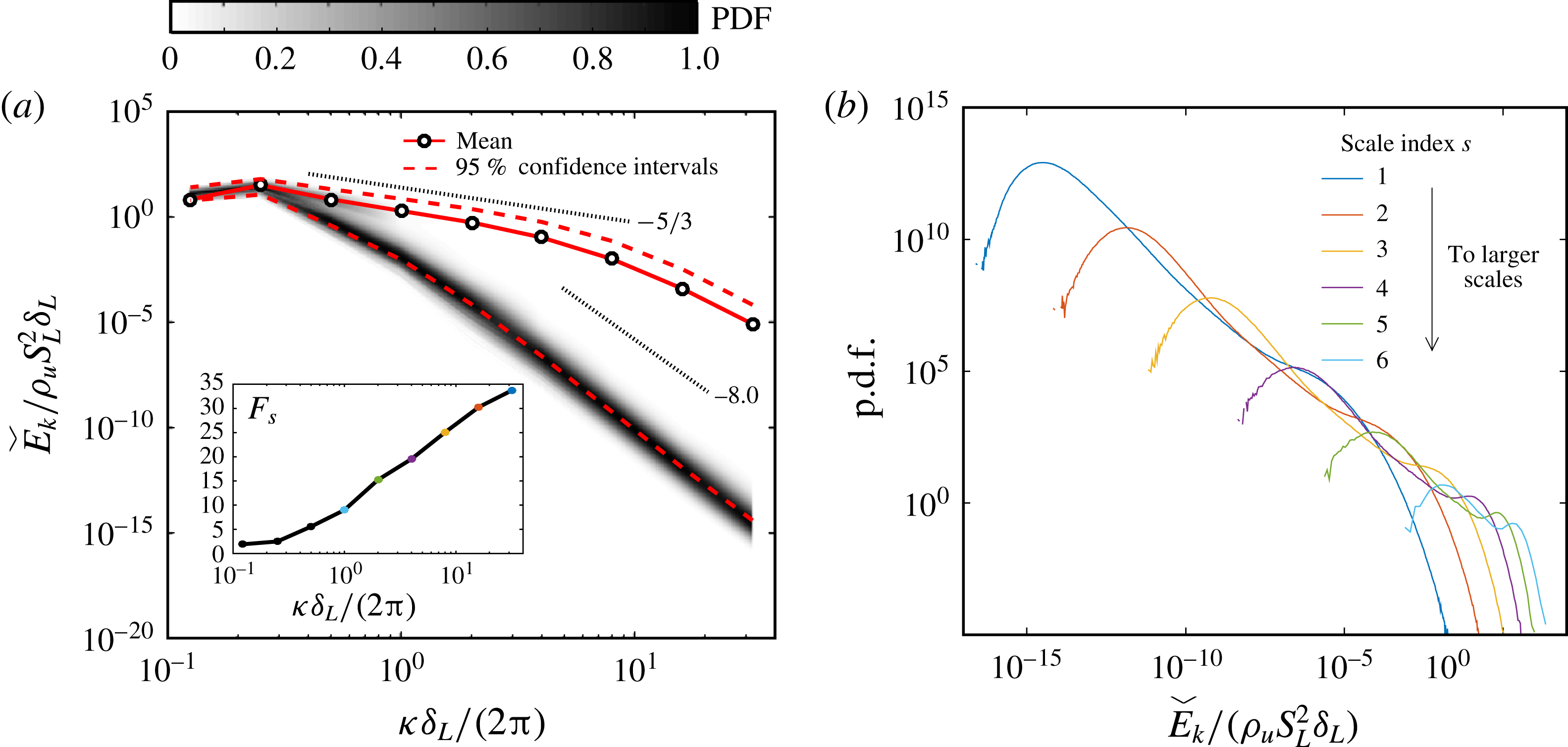
Ensemble-averaged unconditioned probability density functions (PDFs) of the energy spectrum including (a) their projections as solid contours in the spectral plane (rescaled by their corresponding maximum at each scale) and the spectral flatness coefficient (inset), along with (b) cross-sectional cuts at each scale.

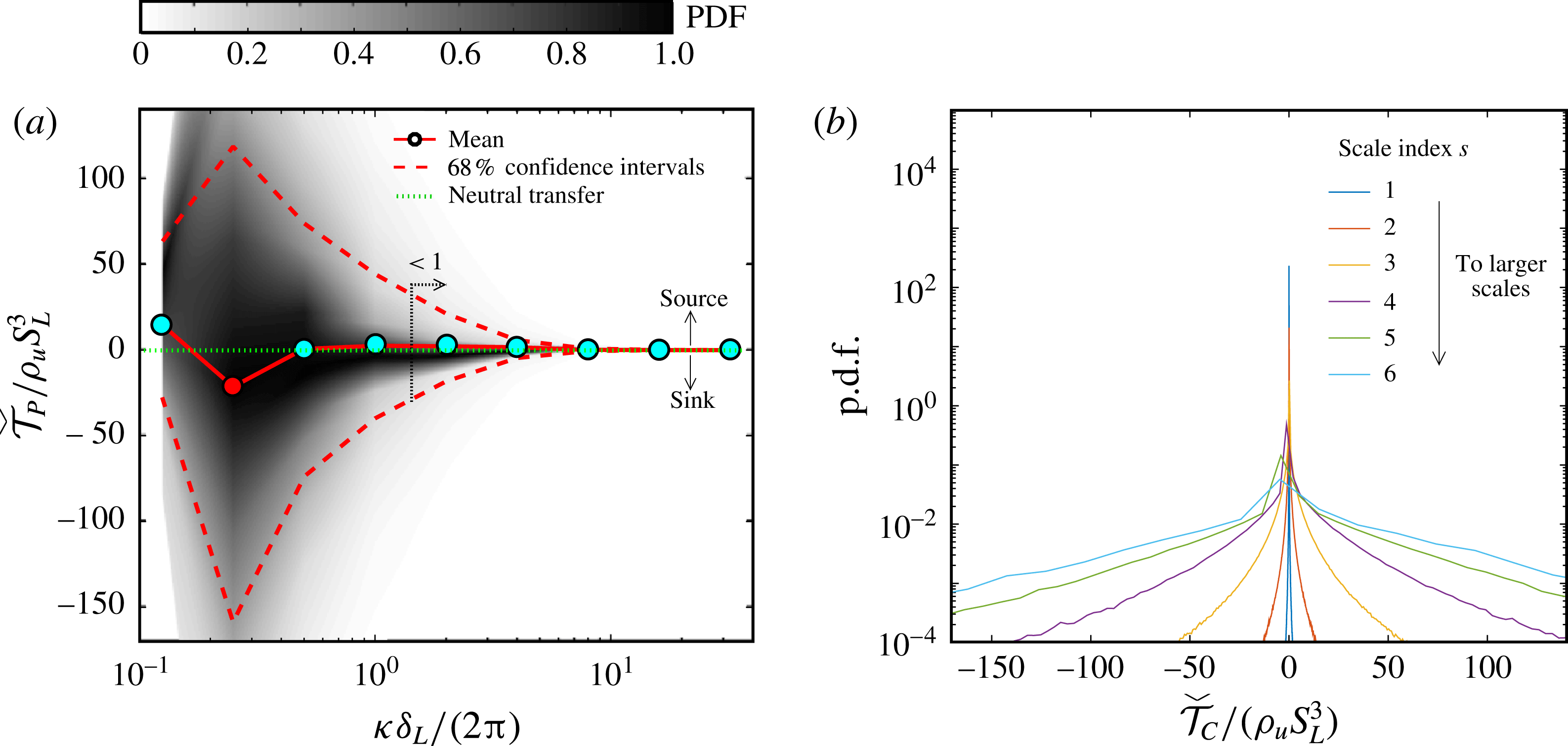
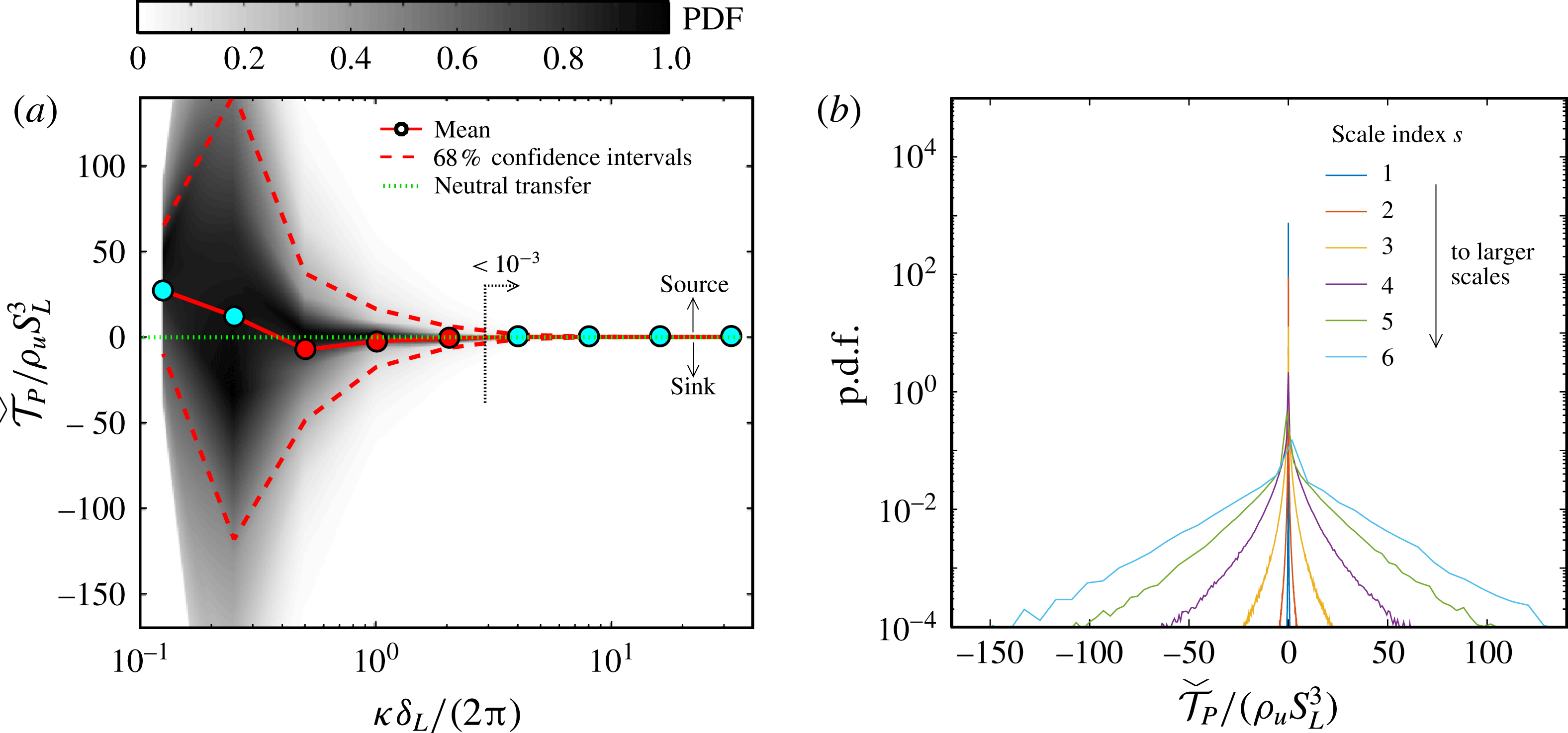
The solid lines in figures 3(a), 4(a) and 5(a) show the mean spectrum
 $\check{E}_{k}(\unicode[STIX]{x1D705})$
and inter-scale fluxes
 $\check{{\mathcal{T}}}_{C}(\unicode[STIX]{x1D705})$
and
 $\check{{\mathcal{T}}}_{P}(\unicode[STIX]{x1D705})$
computed from (5.2)–(5.4) for the DNS case described in § 2. The mean spectrum undergoes the characteristic decay with approximate
 $-5/3$
slope. The mean inter-scale flux by convection,
 $\check{{\mathcal{T}}}_{C}$
, has the largest variations at the large scales, and it flattens thereafter with a positive short-amplitude long tail as the wavenumber increases in a way that resembles the spectral dynamics observed in homogeneous turbulent flows, although in the present configuration
 $\check{{\mathcal{T}}}_{C}$
is not conservative, as explained in § 4. In particular, the scale
 $s=8$
persistently loses energy (
 $\check{{\mathcal{T}}}_{C}<0$
) while the smaller scales (
 $s<8$
) gain energy (
 $\check{{\mathcal{T}}}_{C}>0$
). The largest scale,
 $s=9$
, gains energy by convection and pressure gradient in the volume sampled by the wavelet transform, a pattern that is further investigated in §§ 7 and 8 using conditioned statistics. The mean inter-scale flux of energy due to the pressure gradient,
 $\check{{\mathcal{T}}}_{P}$
, persistently extracts energy from scales
 $s=6$
–
 $7$
around the characteristic flame scale and injects energy into all other scales. The latter corresponds to a mechanism of kinetic-energy delivery by the negative pressure gradient across the flame, which is fundamentally related to the flow acceleration across the front by the momentum equation (O’Brien et al.
Reference O’Brien, Towery, Hamlington, Ihme, Poludnenko and Urzay2017).
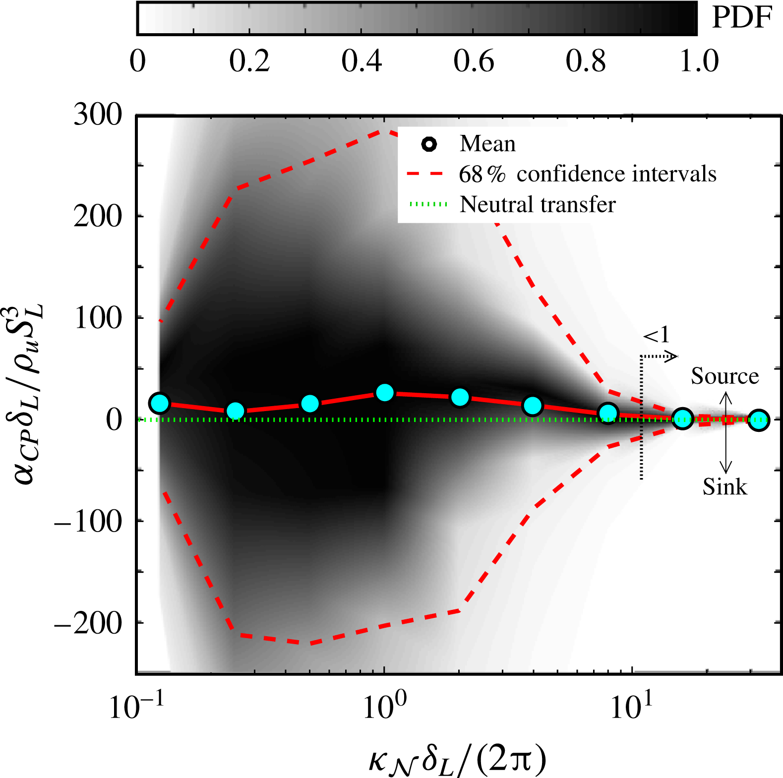
Ensemble-averaged unconditioned PDFs of the convective inter-scale flux including (a) their projections as solid contours in the spectral plane (rescaled by their corresponding maximum at each scale) and (b) cross-sectional cuts at each scale. (a) The cyan- and red-coloured data points indicate respectively positive and negative values of the mean flux, which correspondingly cause an increase and a decrease of kinetic energy on average at the associated wavenumber. The arrow denotes that all mean absolute values to the right of that abscissa are smaller than the indicated value.

Ensemble-averaged unconditioned PDFs of the pressure-gradient inter-scale flux including (a) their projections as solid contours in the spectral plane (rescaled by their corresponding maximum at each scale) and (b) cross-sectional cuts at each scale. (a) The cyan- and red-coloured data points indicate respectively positive and negative values of the mean flux, which correspondingly cause an increase and a decrease of kinetic energy on average at the associated wavenumber. The arrow denotes that all mean absolute values to the right of that abscissa are smaller than the indicated value.

The spectral results described above pertain to the whole turbulent flow field in the mean. Departures from these mean results are significant when the spatial variabilities enabled by the wavelet transform are examined. To see this, consider removing the bracketed operators in (5.2) and (5.4), which leads to local values of the spectrum and the inter-scale fluxes that are given by
 $$\begin{eqnarray}\displaystyle \check{E}_{k}[\unicode[STIX]{x1D705},\boldsymbol{x}_{\boldsymbol{s}}]=\frac{2^{-2s}\unicode[STIX]{x1D6E5}}{4\unicode[STIX]{x03C0}\ln 2}\mathop{\sum }_{d=1}^{7}\check{U}_{i}^{(s,d)}[\boldsymbol{x}_{\boldsymbol{s}}]\check{U}_{i}^{(s,d)}[\boldsymbol{x}_{\boldsymbol{s}}] & & \displaystyle\end{eqnarray}$$
and
 $$\begin{eqnarray}\displaystyle \check{{\mathcal{T}}}_{X}[\unicode[STIX]{x1D705},\boldsymbol{x}_{\boldsymbol{s}}]=\frac{2^{-2s}\unicode[STIX]{x1D6E5}}{2\unicode[STIX]{x03C0}\ln 2}\check{T}_{X}^{(s)}[\boldsymbol{x}_{\boldsymbol{ s}}]. & & \displaystyle\end{eqnarray}$$
At a given wavenumber
 $\unicode[STIX]{x1D705}$
representative of the scale index
 $s$
, the spatial variabilities of
 $\check{E}_{k}$
and
 $\check{{\mathcal{T}}}_{X}$
on the corresponding wavelet-collocation grid
 $\boldsymbol{x}_{\boldsymbol{s}}$
render PDFs whose contours are shown in figures 3–5. In particular, the spatial variabilities of the spectrum are characterized here by the 2.5th and 97.5th percentiles (i.e. approximately four standard deviations of a Gaussian distribution), while the percentiles for the variabilities of the inter-scale fluxes are the 16th and the 84th (i.e. approximately two standard deviations of a Gaussian distribution), in such a way that both sets delimit the interval of values that is observed with 95 % and 68 % frequency in the flow field respectively. It should be noted that the number of samples employed to build the PDFs at the smallest scale
 $s=1$
(or, equivalently,
 $\unicode[STIX]{x1D705}\unicode[STIX]{x1D6FF}_{L}/2\unicode[STIX]{x03C0}=32$
) is 67 000 000 wavelet-collocation points multiplied by
 $15$
snapshots (i.e.
 ${\sim}1000\,000\,000$
samples), whereas the number of samples at the largest scale
 $s=9$
(or, equivalently,
 $\unicode[STIX]{x1D705}\unicode[STIX]{x1D6FF}_{L}/2\unicode[STIX]{x03C0}=0.12$
) is given by four wavelet-collocation points multiplied by
 $15$
snapshots (i.e.
 $60$
samples), in such a way that the large scales are always more difficult to converge statistically. Nonetheless, convergence tests were performed that did not show significant variations of the first- and second-order statistics at
 $s=9$
when the number of snapshots was consecutively increased from 10 to 15.
Following the definition (5.5), figure 3(a) shows interpolated solid contours of the local spectrum
 $\check{E}_{k}(\unicode[STIX]{x1D705},\boldsymbol{x}_{\boldsymbol{s}})$
PDFs normalized by their maxima at each scale. The results indicate that the spatial variabilities of the spectrum with respect to the mean are most pronounced at high wavenumbers, where most wavelet coefficients are small except for a few that correspond to relatively energetic structures setting the mean value far above the mode of the PDF. At least two causes are responsible for the modes of the PDFs of
 $\check{E}_{k}(\unicode[STIX]{x1D705},\boldsymbol{x}_{\boldsymbol{s}})$
occurring far below the mean, along a ridge that decreases with a slope of approximately
 $-8$
. First, small scales are known to have higher intermittency, which is quantitatively ratified by the scale-conditioned flatness
 $F_{s}$
of the spectrum PDF. Specifically,
 $F_{s}$
increases from near-Gaussian values
 $F_{s}\sim 3$
at the large scales to
 $F_{s}\sim 30$
–
 $35$
at the small scales, as observed in the inset of figure 3(a). Correspondingly, the individual PDFs of the spectrum per scale shown in figure 3(b) have increasingly longer tails as the characteristic length (or scale index) decreases. Second, the intermittency of the small scales is also influenced here by the fact that these statistics are obtained by sampling the entire flow field, including the burnt and unburnt sides of the flame, where the turbulence has very different characteristics. This is manifested by the slightly bi-modal character of the PDFs in figure 3(b). It is shown in § 6 using statistics conditioned on the progress variable that the low-energy population of wavelet coefficients along the
 $-8$
-slope ridge mostly belongs to the burnt side of the flame, where the energy of the small scales has plummeted.
The interpolated PDF contours of
 $\check{{\mathcal{T}}}_{C}(\unicode[STIX]{x1D705},\boldsymbol{x}_{\boldsymbol{s}})$
and
 $\check{{\mathcal{T}}}_{P}(\unicode[STIX]{x1D705},\boldsymbol{x}_{\boldsymbol{s}})$
, along with their slices per scale, are shown in figures 4 and 5. The spatial variabilities are maximum at
 $s=8$
in both cases and rapidly decrease with increasing wavenumbers, thereby suggesting that these energy fluxes are primarily active at intermediate-to-large scales, as is expected from the diminishing importance of convection at small scales and the absence of high-wavenumber pressure gradients in this configuration. Nevertheless, the PDFs of
 $\check{{\mathcal{T}}}_{C}(\unicode[STIX]{x1D705},\boldsymbol{x}_{\boldsymbol{s}})$
and
 $\check{{\mathcal{T}}}_{P}(\unicode[STIX]{x1D705},\boldsymbol{x}_{\boldsymbol{s}})$
, divided by the widths of their corresponding 68 % confidence intervals per scale, have increasingly larger widths as the wavenumber increases (not shown here for brevity), which, similarly to the discussion above within the context of
 $\check{E}_{k}(\unicode[STIX]{x1D705},\boldsymbol{x}_{\boldsymbol{s}})$
, highlights the larger relative intermittency present in the small scales with regard to spectral energy-transfer dynamics. It should be noted that the PDF contours of
 $\check{{\mathcal{T}}}_{C}(\unicode[STIX]{x1D705},\boldsymbol{x}_{\boldsymbol{s}})$
and
 $\check{{\mathcal{T}}}_{P}(\unicode[STIX]{x1D705},\boldsymbol{x}_{\boldsymbol{s}})$
in figures 4 and 5 are subject to contributions from both burnt and unburnt gases. The following section introduces a method for separating these contributions by conditioning the fluxes on the local instantaneous progress variable.
6 Method for conditioning spectral statistics on the progress variable
The statistics depicted in figures 3–5 illustrate spatial variabilities of spectral quantities in the entire domain and are unique to the spatial localization properties of the wavelet transform. However, in turbulent premixed combustion, rather than using spatial coordinates, it is more insightful to employ a scalar variable indicating the relative position within the flame front to condition the statistics. In this section, the formulation provided above is generalized to compute the spatial variabilities of spectral quantities conditioned on the local instantaneous progress variable
 $C$
, whose isosurfaces are shown in figure 1.
Since
 $C$
is a function of the spatial coordinates, the conditioning on
 $C$
is not exempt from the constraints imposed by the uncertainty principle discussed in § 3.1. In particular, the conditioning on a particular value
 $C=C_{0}$
defined on the primitive grid
 $\boldsymbol{x}_{\mathbf{0}}$
is subject to an increasingly large spatial delocalization as the length scale
 $\ell _{s}$
increases. Physically, eddies of characteristic length
 $\ell _{s}$
sweep across comparable portions of the progress-variable field near the front in these simulations. As a result, the elements of the wavelet-collocation grids
 $\boldsymbol{x}_{\boldsymbol{s}}$
are bound to include many values of
 $C$
per scale, with an increasingly larger number of them residing in each element of
 $\boldsymbol{x}_{\boldsymbol{s}}$
as
 $\ell _{s}$
increases, and which may or may not include
 $C_{0}$
.
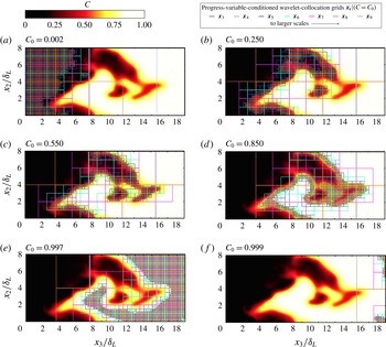
Instantaneous contours of the progress variable
 $C$
superposed on streamwise two-dimensional cross-sections of wavelet-collocation grids
 $\boldsymbol{x}_{\boldsymbol{s}}|(C=C_{0})$
employed to generate the spectral statistics conditioned on
 $C=C_{0}$
, with
 $C_{0}$
being indicated in the upper left corner of each panel. The wavelet-collocation grids for scales
 $s<3$
make the plot too dense and are not shown in order to facilitate visualization of the underlying contours. The streamwise length of the visualization domain shown here is approximately 60 % of the full wavelet-analysis grid.

The considerations given above are summarized in figure 6, which illustrates the way in which statistical conditioning is performed in this study. Specifically, given an arbitrary value of the progress variable
 $C_{0}$
, the spectral data are read only from wavelet-collocation grid elements
 $\boldsymbol{x}_{\boldsymbol{s}}|(C=C_{0})$
such that
 $C_{0}$
lies within the local extrema values of
 $C[\boldsymbol{x}_{\mathbf{0}}]$
determined by the DNS points enveloped by those wavelet-collocation grid elements. For instance, consider the elements
 $\boldsymbol{x}_{\boldsymbol{s}}|(C=0.550)$
used to condition statistics in figure 6(c). The small-scale grid elements activated by the conditioning are well localized within the front region and sweep it from the preheat to the post-flame zones as
 $C$
is increased. On the other hand, the large-scale elements activated by the conditioning are delocalized as prescribed by the uncertainty principle, and in many instances are also activated when not too different values from
 $C$
are chosen for conditioning, as evidenced by comparing the similar elements of
 $\boldsymbol{x}_{\mathbf{8}}$
and
 $\boldsymbol{x}_{\mathbf{9}}$
simultaneously activated in panels (b) and (c) corresponding to
 $C_{0}=0.250$
and
 $0.550$
. Although several other ways may be envisioned to extract conditioned statistics, visual inspections of the grid elements activated by the present method suggest that it appropriately tracks the main features of the highly corrugated turbulent flame as
 $C$
is varied.
The spectral data read from the conditioned wavelet-collocation grid elements
 $\boldsymbol{x}_{\boldsymbol{s}}|(C=C_{0})$
define the progress-variable-conditioned values of the kinetic-energy spectrum and inter-scale fluxes, namely
 $$\begin{eqnarray}\check{E}_{k}[\unicode[STIX]{x1D705},\boldsymbol{x}_{\boldsymbol{s}}|(C=C_{0})]=\frac{2^{-2s}\unicode[STIX]{x1D6E5}}{4\unicode[STIX]{x03C0}\ln 2}\mathop{\sum }_{d=1}^{7}\check{U}_{i}^{(s,d)}[\boldsymbol{x}_{\boldsymbol{ s}}|(C=C_{0})]\check{U}_{i}^{(s,d)}[\boldsymbol{x}_{\boldsymbol{ s}}|(C=C_{0})]\end{eqnarray}$$
and
 $$\begin{eqnarray}\check{{\mathcal{T}}}_{X}[\unicode[STIX]{x1D705},\boldsymbol{x}_{\boldsymbol{s}}|(C=C_{0})]=\frac{2^{-2s}\unicode[STIX]{x1D6E5}}{2\unicode[STIX]{x03C0}\ln 2}\check{T}_{X}^{(s)}[\boldsymbol{x}_{\boldsymbol{ s}}|(C=C_{0})],\end{eqnarray}$$
with
 $X=C$
,
 $P$
,
 $V$
or
 $F$
depending on whether the transfer originates from convective, pressure, viscous or forcing terms. Conditional means of (6.1) and (6.2) can be easily derived by averaging them over the wavelet-collocation grids
 $\boldsymbol{x}_{\boldsymbol{s}}|(C=C_{0})$
in a manner analogous to that introduced in § 5 (i.e. (5.2) and (5.4)).
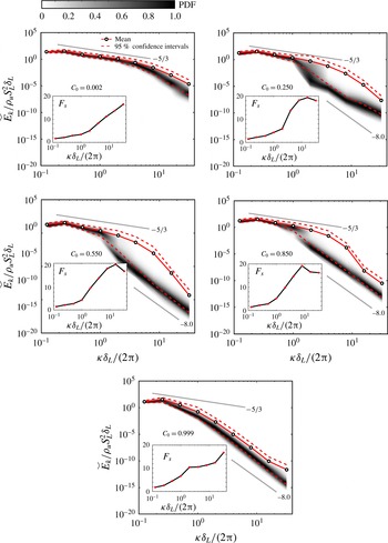
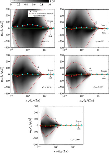
Ensemble-averaged PDF contours conditioned on the progress variable
 $C=C_{0}$
for the energy spectrum, including spectral flatness coefficients (insets).

Ensemble-averaged PDF contours conditioned on the progress variable
 $C=C_{0}$
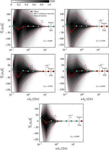
for the convective inter-scale energy flux. The cyan- and red-coloured data points indicate respectively positive and negative values of the conditional mean flux, which correspondingly cause an increase and a decrease of kinetic energy on average at the associated wavenumber. The arrows denote that all mean absolute values to the right of that abscissa are smaller than the indicated value.

7 Energy spectrum and inter-scale energy transfer conditioned on the progress variable
Using (6.1) and the conditioning method introduced in the previous section, the means, variabilities and contours of the PDFs of the progress-variable-conditioned energy spectrum (6.1) are shown in figure 7. A precipitous drop of the mode of the spectrum PDF occurs for values of
 $C$
typical of the preheat zone. This drop starts at intermediate scales
 $s\sim 5$
–
 $7$
(close to the characteristic flame scale
 $s=6$
), continues to smaller scales and then propagates upward in scales up to
 $s=8$
as
 $C$
is further increased towards the reacting regions. This is accompanied by an equally sudden increase in the spectral flatness
 $F_{s}$
of the intermediate scales (insets) as a result of the intermittent broadening of the corresponding spectrum PDFs, whose mean values vary much more gradually – in a manner similar to that predicted by the in-plane
 $\{x_{1},x_{2}\}$
Fourier analyses by Towery et al. (Reference Towery, Poludnenko, Urzay, O’Brien, Ihme and Hamlington2016) – and persist far above the mode despite the large decrease of the latter. The sudden drop takes the mode of the spectrum PDFs down to an approximately 8-slope ridge also visible in the unconditioned statistics in figure 3(a), making any remnants of an inertial subrange disappear. In this way, the final spectral state of the products is one where the energy decays rapidly from scales
 $s=1$
–8 along the aforementioned ridge.
Ensemble-averaged PDF contours conditioned on the progress variable
 $C=C_{0}$
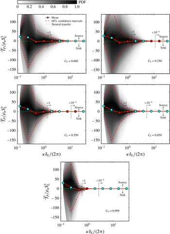
for the pressure-gradient inter-scale energy flux. The cyan- and red-coloured data points indicate respectively positive and negative values of the conditional mean flux, which correspondingly cause an increase and a decrease of kinetic energy on average at the associated wavenumber. The arrows denote that all mean absolute values to the right of that abscissa are smaller than the indicated value.

The progress-variable-conditioned inter-scale energy fluxes due to convection and pressure gradient are shown figures 8 and 9 respectively. In interpreting the results, it is important to note that, although the small values of
 $C$
are in principle associated with the homogeneous–isotropic turbulent flow upstream of the flame, the finite streamwise length of the wavelet-analysis grid makes the conditioned wavelet-collocation grid elements at the largest scale
 $s=9$
remain active near the front even at small values of
 $C$
as a result of the far-reaching long-wavelength front corrugations (see figure 6). As a consequence, the largest scales of the flow conditioned at small values of
 $C$
contain thermal-expansion effects that cause them to be net receptors of energy from both convection and pressure-gradient mechanisms.
The maximum variabilities observed in the PDFs of both energy fluxes are associated with small values of
 $C$
, where the flow field of the fresh gases has the maximum separation of scales, as indicated by the energy spectrum. As
 $C$
is increased, the largest scale
 $s=9$
keeps on receiving energy from both convective and pressure-gradient mechanisms. At values of
 $C$
corresponding to the interior of the flame brush, the convective transfer is found to drain energy primarily from
 $s=8$
while providing energy to the smaller scales. Similarly, the pressure-gradient transfer drains energy primarily from
 $s=7$
and
 $6$
, the latter corresponding to the characteristic flame scale, while injecting energy in all other scales. Although these observations resemble similar ones made within the context of the unconditioned statistics in figures 4 and 5, the conditioning reveals that some of the dynamics, such as the energy drainage from intermediate scales by the pressure gradient, are amplified at intermediate values of
 $C$
. The conditioning of the inter-scale fluxes on near-unity values of
 $C$
leads to a generalized decrease in the mean values at small scales and an attenuation in the spatial variations. Those values of
 $C$
correspond to the burnt gas left far downstream of the flame, which has significantly less separation of scales and flows under mostly neutral dilatation.
The results described above provide quantitative information on the spectrum and inter-scale fluxes conditioned on the progress variable. Since the inter-scale energy fluxes by convection and pressure gradient are created respectively by the flow inertia and thermal-expansion effects near the flame characteristic scale, both of them necessarily decrease in magnitude at small scales. The latter are the scales that are most spatially localized by this wavelet framework, and therefore represent the ones that benefit the most from employing a spatially localized spectral analysis when local multi-scale phenomena are investigated. The spatial localization of the small scales enabled by the wavelet framework is fully exploited in the computation of the cumulative energy transfer of SFS kinetic energy, as shown below.
8 Cumulative transfer of SFS kinetic energy conditioned on the progress variable
Whereas the previous section focuses on the energy spectrum and its rate of variation at a given scale, a quantification of the cumulative transfer of energy into subfilter scales is made below. A supplementary diagram is provided in figure 10 which facilitates the understanding of the computation of this quantity. Consider a high-pass filter such that only the wavelet coefficients for scales
 $s\leqslant {\mathcal{N}}$
are retained, where
 ${\mathcal{N}}$
is a scale index representative of the filter spatial threshold
 $\ell _{{\mathcal{N}}}=2^{{\mathcal{N}}}\unicode[STIX]{x1D6E5}$
, with
 $$\begin{eqnarray}\unicode[STIX]{x1D705}_{{\mathcal{N}}}=2\unicode[STIX]{x03C0}/\ell _{{\mathcal{N}}}\end{eqnarray}$$
an associated cutoff wavenumber. In the corresponding wavelet-collocation grid
 $\boldsymbol{x}_{\boldsymbol{{\mathcal{N}}}}$
, consider a cubic region
 ${\mathcal{M}}_{{\mathcal{N}}}$
of width
 $\ell _{{\mathcal{N}}}$
centred at the particular position
 $\boldsymbol{x}_{\boldsymbol{{\mathcal{N}}}}^{\boldsymbol{p}}$
, through which the local cumulative transfer of energy from all scales smaller than or equal to
 $\ell _{{\mathcal{N}}}$
is to be computed as follows.
Illustration of the computation of the local SFS-cumulative energy flux through a square region
 ${\mathcal{M}}_{{\mathcal{N}}}$
of width
 $\ell _{{\mathcal{N}}}=2^{{\mathcal{N}}}\unicode[STIX]{x1D6E5}$
centred at a spatial position
 $\boldsymbol{x}_{\boldsymbol{{\mathcal{N}}}}^{\boldsymbol{p}}$
across a filter scale cutoff
 ${\mathcal{N}}=3$
. In this example, the grid contains
 $16\times 16$
elements and correspondingly has
 ${\mathcal{S}}=4$
wavelet-decomposition levels.

Since the total number of primitive grid points contained in
 ${\mathcal{M}}_{{\mathcal{N}}}$
is
 $2^{3{\mathcal{N}}}$
, the scale-dependent spatial average of
 $y[\boldsymbol{x}_{\boldsymbol{s}}]$
over wavelet-collocation grid points located within
 ${\mathcal{M}}_{{\mathcal{N}}}$
is
 $\langle y[\boldsymbol{x}_{\boldsymbol{s}}]\rangle _{\boldsymbol{x}_{\boldsymbol{s}}\in {\mathcal{M}}_{{\mathcal{N}}}}=\sum _{\boldsymbol{x}_{\boldsymbol{s}}\in {\mathcal{M}}_{{\mathcal{N}}}}2^{3(s-{\mathcal{N}})}y[\boldsymbol{x}_{\boldsymbol{s}}]$
. As a result,
 $2^{-3(s-{\mathcal{N}})}\langle y[\boldsymbol{x}_{\boldsymbol{s}}]\rangle _{\boldsymbol{x}_{\boldsymbol{s}}\in {\mathcal{M}}_{{\mathcal{N}}}}$
represents the sum of all of the values of
 $y$
across all wavelet-collocation grid points enclosed in
 ${\mathcal{M}}_{{\mathcal{N}}}$
. Upon substituting the arbitrary variable
 $y[\boldsymbol{x}_{\boldsymbol{s}}]$
by the spectral kinetic energy
 $\check{e}^{(s)}[\boldsymbol{x}_{\boldsymbol{s}}]$
and summing from
 $s=1$
to the filter-threshold scale
 $s={\mathcal{N}}$
, the definition of the SFS kinetic energy
 $$\begin{eqnarray}k_{SFS}[\unicode[STIX]{x1D705}_{{\mathcal{N}}},\boldsymbol{x}_{\boldsymbol{{\mathcal{N}}}}^{\boldsymbol{p}}]=\mathop{\sum }_{s=1}^{{\mathcal{N}}}2^{-3(s-{\mathcal{N}})}\langle \check{e}^{(s)}[\boldsymbol{x}_{\boldsymbol{ s}}]\rangle _{\boldsymbol{x}_{\boldsymbol{s}}\in {\mathcal{M}}_{{\mathcal{N}}}}\end{eqnarray}$$
is obtained, which represents the total amount of kinetic energy accumulated in subfilter scales
 $\ell \leqslant \ell _{{\mathcal{N}}}$
locally within the spatial region
 ${\mathcal{M}}_{{\mathcal{N}}}$
. Similarly, a conservation equation for
 $k_{SFS}$
can be derived by summing (4.14) over the interval of scales
 $1\leqslant s\leqslant {\mathcal{N}}$
and spatially averaging over wavelet-collocation grid points
 $\boldsymbol{x}_{\boldsymbol{s}}$
nested in
 ${\mathcal{M}}_{{\mathcal{N}}}$
, which gives
 $$\begin{eqnarray}\displaystyle \frac{\unicode[STIX]{x2202}}{\unicode[STIX]{x2202}t}k_{SFS}[\unicode[STIX]{x1D705}_{{\mathcal{N}}},\boldsymbol{x}_{\boldsymbol{{\mathcal{N}}}}^{\boldsymbol{p}}]=\unicode[STIX]{x1D6FC}_{C}[\unicode[STIX]{x1D705}_{{\mathcal{N}}},\boldsymbol{x}_{\boldsymbol{{\mathcal{N}}}}^{\boldsymbol{p}}]+\unicode[STIX]{x1D6FC}_{P}[\unicode[STIX]{x1D705}_{{\mathcal{N}}},\boldsymbol{x}_{\boldsymbol{{\mathcal{N}}}}^{\boldsymbol{p}}]+\unicode[STIX]{x1D6FC}_{V}[\unicode[STIX]{x1D705}_{{\mathcal{N}}},\boldsymbol{x}_{\boldsymbol{{\mathcal{N}}}}^{\boldsymbol{p}}]+\unicode[STIX]{x1D6FC}_{F}[\unicode[STIX]{x1D705}_{{\mathcal{N}}},\boldsymbol{x}_{\boldsymbol{{\mathcal{N}}}}^{\boldsymbol{p}}]. & & \displaystyle\end{eqnarray}$$
In this formulation, the terms
 $\unicode[STIX]{x1D6FC}_{X}$
represent the local cumulative flux of SFS kinetic energy
 $$\begin{eqnarray}\unicode[STIX]{x1D6FC}_{X}[\unicode[STIX]{x1D705}_{{\mathcal{N}}},\boldsymbol{x}_{\boldsymbol{{\mathcal{N}}}}^{\boldsymbol{p}}]=\mathop{\sum }_{s=1}^{{\mathcal{N}}}2^{-3(s-{\mathcal{N}})}\langle \check{T}_{X}^{(s)}[\boldsymbol{x}_{\boldsymbol{ s}}]\rangle _{\boldsymbol{x}_{\boldsymbol{s}}\in {\mathcal{M}}_{{\mathcal{N}}}},\end{eqnarray}$$
with
 $X=C$
,
 $P$
,
 $V$
or
 $F$
depending on whether the transfer mechanism is related to convective, pressure, viscous or forcing terms, as in (4.15)–(4.18). In the results presented below, emphasis is placed on the sum
 $\unicode[STIX]{x1D6FC}_{C}[\unicode[STIX]{x1D705}_{{\mathcal{N}}},\boldsymbol{x}_{\boldsymbol{{\mathcal{N}}}}^{\boldsymbol{p}}]+\unicode[STIX]{x1D6FC}_{P}[\unicode[STIX]{x1D705}_{{\mathcal{N}}},\boldsymbol{x}_{\boldsymbol{{\mathcal{N}}}}^{\boldsymbol{p}}]$
, which represents the combined action of convection and pressure gradient and is given by
 $$\begin{eqnarray}\displaystyle \unicode[STIX]{x1D6FC}_{CP}[\unicode[STIX]{x1D705}_{{\mathcal{N}}},\boldsymbol{x}_{\boldsymbol{{\mathcal{N}}}}^{\boldsymbol{p}}] & = & \displaystyle \unicode[STIX]{x1D6FC}_{C}[\unicode[STIX]{x1D705}_{{\mathcal{N}}},\boldsymbol{x}_{\boldsymbol{{\mathcal{N}}}}^{\boldsymbol{p}}]+\unicode[STIX]{x1D6FC}_{P}[\unicode[STIX]{x1D705}_{{\mathcal{N}}},\boldsymbol{x}_{\boldsymbol{{\mathcal{N}}}}^{\boldsymbol{p}}]\nonumber\\ \displaystyle & = & \displaystyle \mathop{\sum }_{s=1}^{{\mathcal{N}}}2^{-3(s-{\mathcal{N}})}\langle \check{T}_{C}^{(s)}[\boldsymbol{x}_{\boldsymbol{s}}]+\check{T}_{P}^{(s)}[\boldsymbol{x}_{\boldsymbol{s}}]\rangle _{\boldsymbol{x}_{\boldsymbol{s}}\in {\mathcal{M}}_{{\mathcal{N}}}}.\end{eqnarray}$$
In these simulations, the convective and pressure-gradient terms participating in (8.5) are observed to be of the same order of magnitude.
Unconditioned ensemble-averaged PDF contours of the local cumulative flux (8.5) of SFS kinetic energy due to convection and pressure-gradient mechanisms of momentum transport as a function of the cutoff wavenumber
 $\unicode[STIX]{x1D705}_{{\mathcal{N}}}$
. The cyan-coloured data points indicate positive values of the mean flux, which correspondingly cause an increase in SFS kinetic energy on average. The arrow denotes that all mean absolute values to the right are smaller than the indicated value.

The physical interpretation of the local cumulative flux of SFS kinetic energy (8.5) is as follows. Based on the SFS kinetic-energy conservation equation (8.3), positive values
 $\unicode[STIX]{x1D6FC}_{CP}[\unicode[STIX]{x1D705}_{{\mathcal{N}}},\boldsymbol{x}_{\boldsymbol{{\mathcal{N}}}}^{\boldsymbol{p}}]>0$
indicate net gain of SFS kinetic energy caused by convection and pressure-gradient mechanisms through the spatial region
 ${\mathcal{M}}_{{\mathcal{N}}}$
, centred at
 $\boldsymbol{x}_{\boldsymbol{{\mathcal{N}}}}^{\boldsymbol{p}}$
, and across a scale
 ${\mathcal{N}}$
corresponding to the representative wavenumber
 $\unicode[STIX]{x1D705}_{{\mathcal{N}}}$
. In a similar way, negative values
 $\unicode[STIX]{x1D6FC}_{CP}[\unicode[STIX]{x1D705}_{{\mathcal{N}}},\boldsymbol{x}_{\boldsymbol{{\mathcal{N}}}}^{\boldsymbol{p}}]<0$
correspond to a local loss of SFS kinetic energy through the same spatial region, centred at the same location, and across the same scale as before. In addition, a relevant property of (8.5) is that the sum of
 $\unicode[STIX]{x1D6FC}_{CP}$
over all positions
 $\boldsymbol{x}_{\boldsymbol{{\mathcal{N}}}}$
is equivalent to the integral of the corresponding mean inter-scale flux from the smallest scale to the filter threshold
 ${\mathcal{N}}$
, namely
 $$\begin{eqnarray}2^{-3{\mathcal{N}}}\langle \unicode[STIX]{x1D6FC}_{CP}[\unicode[STIX]{x1D705}_{{\mathcal{N}}},\boldsymbol{x}_{\boldsymbol{{\mathcal{N}}}}^{\boldsymbol{p}}]\rangle _{\boldsymbol{ x}_{\boldsymbol{{\mathcal{N}}}}}=\mathop{\sum }_{\unicode[STIX]{x1D73F}}^{\unicode[STIX]{x1D705}_{{\mathcal{N}}}}[\check{{\mathcal{T}}}_{C}(\unicode[STIX]{x1D73F})+\check{{\mathcal{T}}}_{P}(\unicode[STIX]{x1D73F})]\unicode[STIX]{x1D6FF}\unicode[STIX]{x1D705},\end{eqnarray}$$
as observed by combining (3.10), (3.11), (5.4) and (8.5).
The contours of the unconditioned PDFs of
 $\unicode[STIX]{x1D6FC}_{CP}(\unicode[STIX]{x1D705}_{{\mathcal{N}}},\boldsymbol{x}_{\boldsymbol{{\mathcal{N}}}})$
are shown in figure 11 for different filter wavenumber thresholds
 $\unicode[STIX]{x1D705}_{{\mathcal{N}}}$
. The results resemble those reported for incompressible homogeneous–isotropic turbulent flows in Meneveau (Reference Meneveau1991). Notwithstanding the complex inter-scale energy-transfer dynamics that may be observed in figures 4 and 5, the cumulative outcome is that energy is transferred by convection and pressure-gradient mechanisms into subfilter scales on average and independently of the filter threshold when the flow is analysed on the whole, including both reactants and products, in a way that qualitatively resembles the direct energy cascade. This trend, however, is subject to significant dispersion, as evidenced by the large variabilities from the mean which include a large number of spatial locations in the domain where
 $\unicode[STIX]{x1D6FC}_{CP}<0$
, causing the SFS kinetic energy to decrease. Further insight into the origin of these variabilities can be gained by conditioning
 $\unicode[STIX]{x1D6FC}_{CP}$
on the local progress variable as follows.
Ensemble-averaged PDF contours conditioned on the progress variable
 $C=C_{0}$
for the local cumulative flux (8.5) of SFS kinetic energy due to convection and pressure-gradient mechanisms of momentum transport as a function of the cutoff wavenumber
 $\unicode[STIX]{x1D705}_{{\mathcal{N}}}$
. The cyan- and red-coloured data points indicate respectively positive and negative values of the conditional mean flux, which correspondingly cause an increase and a decrease of SFS kinetic energy on average. The arrows denote that all mean absolute values to the right of that abscissa are smaller than the indicated value.

The local cumulative flux of SFS kinetic energy conditioned on the progress variable is defined as
 $$\begin{eqnarray}\displaystyle \unicode[STIX]{x1D6FC}_{CP}[\unicode[STIX]{x1D705}_{{\mathcal{N}}},\boldsymbol{x}_{\boldsymbol{s}}|(C=C_{0})]=\mathop{\sum }_{s=1}^{{\mathcal{N}}}2^{-3(s-{\mathcal{N}})}\langle \check{T}_{C}^{(s)}[\boldsymbol{x}_{\boldsymbol{s}}|(C=C_{0})]+\check{T}_{P}^{(s)}[\boldsymbol{x}_{\boldsymbol{s}}|(C=C_{0})]\rangle _{\boldsymbol{x}_{\boldsymbol{s}}\in {\mathcal{M}}_{{\mathcal{N}}}},\quad & & \displaystyle\end{eqnarray}$$
which is obtained by evaluating (8.5) at the conditioned wavelet-collocation grid points, as described in § 6. At small values of
 $C$
, which correspond to the turbulent flow upstream of the flame, the tendency of the conditional mean of the cumulative flux is to replenish SFS kinetic energy, although the spatial variabilities there are the largest, as evidenced by the wide contours of the PDF of
 $\unicode[STIX]{x1D6FC}_{CP}$
for
 $C=0.002$
in figure 12. However, in contrast to the strictly positive values of the unconditioned
 $\unicode[STIX]{x1D6FC}_{CP}$
, the mean of its conditioned version (8.7) changes sign as
 $C$
increases, and becomes negative in some cases. This occurs most intensely for sufficiently large filter sizes
 $\ell _{{\mathcal{N}}}$
with
 ${\mathcal{N}}=7$
–
 $9$
, which correspond to scales similar to or larger than the flame thickness, as shown by the red circles in figure 12 indicating local drainage of SFS kinetic energy for the cases
 $C\geqslant 0.250$
in a conditional-average sense.
The results presented above suggest that, when
 ${\mathcal{N}}$
is larger than the flame characteristic scale, convection and pressure-gradient mechanisms drain significant amounts of SFS kinetic energy at a local mean rate approximately of order
 $10\unicode[STIX]{x1D70C}_{u}S_{L}^{3}/\unicode[STIX]{x1D6FF}_{L}\sim 10\unicode[STIX]{x1D70C}_{u}\unicode[STIX]{x1D716}Da(S_{L}/u_{\ell })^{2}$
, where
 $\unicode[STIX]{x1D716}$
is the overall mean dissipation. However, caution should be exercised in interpreting this reverse energy flux as a purely energy-backscatter phenomenon understood as an energy transfer in the direction from small to large scales. Specifically,
 $\unicode[STIX]{x1D6FC}_{CP}$
may not solely account for energy transfer across the filter scale
 ${\mathcal{N}}$
, but it may also account for energy transfer from adjacent positions at the same scale level. To see this, note that
 $\unicode[STIX]{x1D6FC}_{CP}$
relies on the energy fluxes
 $\check{T}_{C}^{(s)}[\boldsymbol{x}_{\boldsymbol{s}}]$
and
 $\check{T}_{P}^{(s)}[\boldsymbol{x}_{\boldsymbol{s}}]$
. Despite the fact that these energy fluxes are locally evaluated in space, they require information on
 $u_{i}$
,
 $U_{i}$
,
 $\unicode[STIX]{x1D70C}$
and
 $P$
from at least three positions at the cutoff scale level
 ${\mathcal{N}}$
, as evidenced by (4.19) and (4.20). As a consequence, if eddies were associated with fluctuations in those primitive variables, energy transfer from other spatial locations into
 ${\mathcal{M}}_{{\mathcal{N}}}$
might occur that would also be included in
 $\unicode[STIX]{x1D6FC}_{CP}$
, and that would not be necessarily related to energy transfer across the cutoff scale
 ${\mathcal{N}}$
. In triply periodic turbulent flows, it is plausible that the spatially averaged local cumulative energy flux, defined by
 $$\begin{eqnarray}\unicode[STIX]{x1D6FC}_{CP}(\unicode[STIX]{x1D705}_{{\mathcal{N}}})=\mathop{\sum }_{s=1}^{{\mathcal{N}}}2^{-3(s-{\mathcal{N}})}\langle \langle \check{T}_{C}^{(s)}[\boldsymbol{x}_{\boldsymbol{ s}}]+\check{T}_{P}^{(s)}[\boldsymbol{x}_{\boldsymbol{ s}}]\rangle _{\boldsymbol{x}_{\boldsymbol{s}}\in {\mathcal{M}}_{{\mathcal{N}}}}\rangle _{\boldsymbol{x}_{\boldsymbol{{\mathcal{N}}}}},\end{eqnarray}$$
represents a quantity that can isolate the cross-scale transfer (i.e. across the cutoff scale
 ${\mathcal{N}}$
) because the cross-spatial contributions at the scale index
 ${\mathcal{N}}$
are cancelled upon averaging. In non-periodic flows such as the one investigated here, or in progress-variable-conditioned zones of the flow, which correspond to regions of limited spatial extent, the additional cross-spatial transfer may advise against strictly stating within the context of the results presented in figure 12 that all of the kinetic energy drained from the subfilter scales at a given location is transferred to the superfilter scales at that same location across the scale of the filter. More refined descriptions that attempt to suppress the cross-spatial transfer at the cutoff level are available for incompressible flows in the form of a dual bi-spectrum of transfer (Meneveau Reference Meneveau1991). Nonetheless, to the best of the authors’ knowledge, a unique way of defining a wavelet-based dual bi-spectrum of transfer does not seem to exist in compressible turbulent flows, and a clear physical-space energy-flux counterpart upon which to rely for a physical interpretation of this quantity cannot be straightforwardly defined. Further investigation into these advanced aspects is the subject of future work.
9 Conclusions
In this study, a 3D wavelet multi-resolution analysis is carried out to investigate the spatially localized transfer of kinetic energy across scales in turbulent premixed flames obtained from DNS at a turbulent intensity of 7.8 and a Karlovitz number of 72. Specifically, the DNS computational set-up involves a premixed flame propagating in forced homogeneous–isotropic turbulence along a cuboidal unconfined domain with periodic boundary conditions in the transverse directions.
The wavelet-space energetics formulation for incompressible turbulent flows proposed by Meneveau (Reference Meneveau1991) is extended here to compressible chemically reacting turbulent non-periodic flows conditioned on the progress variable and integrated in cuboidal domains. In constant- and variable-density homogeneous–isotropic turbulent flows integrated in triply periodic cubic domains, the resulting formalism leads to conservation of the convective inter-scale fluxes and warrants the collapse of the spectral energy equation on the well-known balance equation for the mean turbulent kinetic energy in physical space.
Results similar to those previously reported for incompressible turbulent flows are observed when the flow is analysed on the whole, including both the unburnt and burnt sides of the flame. In particular, the convective and pressure-gradient inter-scale fluxes tend to drain or neutralize the energy of the large scales and increase the energy of the small scales. However, richer dynamics are unveiled when examining particular regions of space representative of the flame front at different scales, which are discriminated using a method for conditioning on the local instantaneous progress variable.
As the progress variable is varied across the flame brush, the conditioned energy spectra are shown to undergo, in most spatial locations, a precipitous drop that begins around the flame characteristic scale, is accompanied by an increase in the spectral flatness and leads to a subsequent depletion of kinetic energy of increasingly larger scales. However, the corresponding decrease in the spatially averaged value of the spectra is much more gradual and resembles that observed in early studies based on two-dimensional Fourier transforms along transverse planes parallel to the mean flame brush.
Convection increases the kinetic energy of the small scales and mostly drains it from the large scales across the flame. However, as elicited by the formulation and observed from the results, the cuboidal shape of the grid and the non-periodic boundary conditions necessarily cause the convective transfer to be non-conservative. As a consequence, physical interpretations of energy-transfer phenomena based on the classic turbulence cascade cannot be straightforwardly employed in the present configuration. In addition, because of thermal expansion across the flame, the pressure-gradient inter-scale flux extracts energy from intermediate scales similar to the flame characteristic scale, and energizes the small and large scales.
The local cumulative transfer of SFS kinetic energy across a cutoff scale imposed by a high-pass wavelet filter is quantified in order to study the conditions under which kinetic energy is injected or drained from the small scales by the combined contribution of convective and pressure-gradient mechanisms of momentum transport. Unconditioned results indicate that SFS kinetic energy is injected in the subfilter scales on average, in a way that resembles the direct cascade observed in incompressible homogeneous–isotropic turbulent flows. However, the local cumulative flux conditioned on the progress variable is shown to drain SFS kinetic energy on average from the small scales within the flame brush by convective and pressure-gradient mechanisms of momentum transport. This occurs most intensely when the cutoff scale, across which the transfer is computed, is larger than the flame characteristic scale. The resulting reverse energy transfer, which is reminiscent of the physical-space combustion-induced backscatter observed by O’Brien et al. (Reference O’Brien, Towery, Hamlington, Ihme, Poludnenko and Urzay2017) using physical-space filters, tends to be neutralized when the cutoff scale is increased up to the maximum decomposition level corresponding to the spanwise domain length.
It is worth emphasizing that results obtained from spectral-space analyses typically depend on the spectral basis. As a consequence, the conclusions presented in this study are expected to be quantitatively sensitive to that choice. Nonetheless, some of the findings outlined here, such as the variations of the kinetic-energy spectra across the flame or the prevailing drainage of SFS kinetic energy by multi-scale energy-transfer mechanisms related to the convective and pressure-gradient transfer terms, are qualitatively ratified by earlier work on a similar configuration using physical-space and Fourier filters (Towery et al. Reference Towery, Poludnenko, Urzay, O’Brien, Ihme and Hamlington2016; O’Brien et al. Reference O’Brien, Towery, Hamlington, Ihme, Poludnenko and Urzay2017), even though the exact equivalences between these different approaches are not straightforward to quantify. Aspects worthy of future work to clarify some of these open research questions may include (a) the consideration of wider parameter ranges in the combustion-regime diagram which may enable comparisons and elucidation of more general physical trends in flame energetics, (b) the partition of the physical-space flow field into solenoidal and irrotational components to wavelet-analyse each contribution and isolate the role of thermal expansion in the energy transfer, (c) the incorporation of complex chemical effects that are known to be important for the propagation of realistic turbulent flames and (d) the utilization of different and perhaps more practical flow configurations for turbulent combustion, including effects related to externally applied pressure gradients (Veynante & Poinsot Reference Veynante and Poinsot1997), shear layers (Wang et al. Reference Wang, Hawkes, Chen, Zhou, Li and Aldén2017; MacArt, Grenga & Mueller Reference MacArt, Grenga and Mueller2018) and high-speed compressibility phenomena (Urzay Reference Urzay2018).
Acknowledgements
This investigation was funded by the US AFOSR grants # FA9550-14-1-0219 and # FA9550-14-1-0273 managed by Dr C. Li. Computing resources were provided by the US Department of Defense, High-Performance Computing Modernization Program, under a Frontier Award. The authors are grateful to Professor P. Moin, Professor C. Pantano, Dr D. Livescu and Dr L. Jofre for helpful technical discussions.
Appendix A. Wavelet formulation: supplementary definitions
For illustration, consider the simpler case of a 1D finite-energy continuous function
 $y(x)$
defined on the real axis
 $x$
that has no significant contribution from scales smaller than the grid spacing
 $\unicode[STIX]{x1D6E5}$
introduced in the main text. The wavelet series expansion of
 $y(x)$
in semi-discrete form can be written as

where
 $\unicode[STIX]{x1D713}^{(s)}(x-x_{s})$
and
 $\unicode[STIX]{x1D719}^{(s)}(x-x_{s})$
are orthonormal wavelet and scaling functions respectively, which are defined in terms of their scale-independent counterparts
 $\unicode[STIX]{x1D713}$
(mother wavelet) and
 $\unicode[STIX]{x1D719}$
(father scaling function) as
 $$\begin{eqnarray}\unicode[STIX]{x1D713}^{(s)}(x-x_{s})=\ell _{s}^{-1/2}\unicode[STIX]{x1D713}\left(\frac{x-x_{s}}{\ell _{s}}\right),\quad \unicode[STIX]{x1D719}^{(s)}(x-x_{s})=\ell _{s}^{-1/2}\unicode[STIX]{x1D719}\left(\frac{x-x_{s}}{\ell _{s}}\right),\end{eqnarray}$$
where
 $\ell _{s}=2^{s}\unicode[STIX]{x1D6E5}$
is the characteristic length of the wavelet at scale
 $s$
(also defined in (3.10) in the main text). In this study,
 $\unicode[STIX]{x1D713}$
and
 $\unicode[STIX]{x1D719}$
are taken to be wavelet and scaling functions of the Daubechies family (Daubechies Reference Daubechies1992).
Upon multiplying both sides of the expansion (A 1) by the scaling function
 $\unicode[STIX]{x1D719}^{(0)}$
 $(x-x_{0})$
at the zeroth (grid-resolution
 $\unicode[STIX]{x1D6E5}$
) scale, integrating along
 $x$
and using the standard approximation (Meneveau Reference Meneveau1990; Addison Reference Addison2002)

to compute the first approximation coefficient  , a discrete analogue of the above series expansion,

is obtained that resembles the 1D version of (3.2), where the discrete wavelet and scaling functions can be expressed as (Meneveau Reference Meneveau1990, Reference Meneveau1991)
 $$\begin{eqnarray}g^{(s)}[x_{0}-x_{s}]=\unicode[STIX]{x1D6E5}^{-1/2}\int _{-\infty }^{\infty }\unicode[STIX]{x1D713}^{(s)}(x-x_{s})\unicode[STIX]{x1D719}^{(0)}(x-x_{0})\,\text{d}x\end{eqnarray}$$
and
 $$\begin{eqnarray}h^{({\mathcal{S}})}[x_{0}-x_{{\mathcal{S}}}]=\unicode[STIX]{x1D6E5}^{-1/2}\int _{-\infty }^{\infty }\unicode[STIX]{x1D719}^{({\mathcal{S}})}(x-x_{{\mathcal{S}}})\unicode[STIX]{x1D719}^{(0)}(x-x_{0})\,\text{d}x.\end{eqnarray}$$
It should be noted that the approximation (A 3) made above can be improved in different ways (Strang & Nguyen Reference Strang and Nguyen1996), including the utilization of Coiflet wavelets (Daubechies Reference Daubechies1993).
Based on the above expressions, and on the additional relation (Mallat Reference Mallat1989)
 $$\begin{eqnarray}\unicode[STIX]{x1D713}^{(s)}(x-x_{s})=\mathop{\sum }_{x_{0}}\left[\int _{-\infty }^{+\infty }\unicode[STIX]{x1D713}^{(s)}(x^{\prime }-x_{s})\unicode[STIX]{x1D719}^{(0)}(x^{\prime }-x_{0})\,\text{d}x^{\prime }\right]\unicode[STIX]{x1D719}^{(0)}(x-x_{0}),\end{eqnarray}$$
the classic orthogonality conditions associated with the continuous wavelet and scaling functions readily lead to corresponding orthogonality constraints for
 $g^{(s)}[x_{0}-x_{s}]$
and
 $h^{(s)}[x_{0}-x_{s}]$
, namely
 $$\begin{eqnarray}\displaystyle & \displaystyle \unicode[STIX]{x1D6E5}\mathop{\sum }_{x_{0}}g^{(s)}[x_{0}-x_{s}]g^{(s^{\prime })}[x_{0}-x_{s^{\prime }}]=\int _{-\infty }^{+\infty }\unicode[STIX]{x1D713}^{(s)}(x-x_{s})\unicode[STIX]{x1D713}^{(s^{\prime })}(x-x_{s^{\prime }})\,\text{d}x=\unicode[STIX]{x1D6FF}_{s,s^{\prime }}\unicode[STIX]{x1D6FF}_{x_{s},x_{s^{\prime }}},\quad & \displaystyle\end{eqnarray}$$
 $$\begin{eqnarray}\displaystyle & \displaystyle \unicode[STIX]{x1D6E5}\mathop{\sum }_{x_{0}}g^{(s)}[x_{0}-x_{s}]h^{({\mathcal{S}})}[x_{0}-x_{{\mathcal{S}}}]=\int _{-\infty }^{+\infty }\unicode[STIX]{x1D713}^{(s)}(x-x_{s})\unicode[STIX]{x1D719}^{({\mathcal{S}})}(x-x_{{\mathcal{S}}})\,\text{d}x=0 & \displaystyle\end{eqnarray}$$
and
 $$\begin{eqnarray}\unicode[STIX]{x1D6E5}\mathop{\sum }_{x_{0}}h^{({\mathcal{S}})}[x_{0}-x_{{\mathcal{S}}}]h^{({\mathcal{S}})}[x_{0}-x_{{\mathcal{S}}}^{\prime }]=\int _{-\infty }^{+\infty }\unicode[STIX]{x1D719}^{({\mathcal{S}})}(x-x_{{\mathcal{S}}})\unicode[STIX]{x1D719}^{({\mathcal{S}})}(x-x_{{\mathcal{S}}}^{\prime })\,\text{d}x=\unicode[STIX]{x1D6FF}_{x_{{\mathcal{S}}},x_{{\mathcal{S}}}^{\prime }}.\end{eqnarray}$$
The discrete 3D wavelet and scaling functions
 ${\mathcal{G}}^{(s,d)}[\boldsymbol{x}_{\mathbf{0}}-\boldsymbol{x}_{\boldsymbol{s}}]$
and
 ${\mathcal{H}}^{({\mathcal{S}})}[\boldsymbol{x}_{\mathbf{0}}-\boldsymbol{x}_{\boldsymbol{{\mathcal{S}}}}]$
used in the discrete wavelet series expansion (3.2) can be constructed from the multiplicative combinations of their 1D counterparts as
 $$\begin{eqnarray}\left.\begin{array}{@{}c@{}}\displaystyle {\mathcal{G}}^{(s,1)}[\boldsymbol{x}_{\mathbf{0}}-\boldsymbol{x}_{\boldsymbol{s}}]=\unicode[STIX]{x1D6E5}^{3/2}g^{(s)}[x_{0,(1)}-x_{s,(1)}]g^{(s)}[x_{0,(2)}-x_{s,(2)}]g^{(s)}[x_{0,(3)}-x_{s,(3)}],\\ \displaystyle {\mathcal{G}}^{(s,2)}[\boldsymbol{x}_{\mathbf{0}}-\boldsymbol{x}_{\boldsymbol{s}}]=\unicode[STIX]{x1D6E5}^{3/2}h^{(s)}[x_{0,(1)}-x_{s,(1)}]g^{(s)}[x_{0,(2)}-x_{s,(2)}]g^{(s)}[x_{0,(3)}-x_{s,(3)}],\\ \displaystyle {\mathcal{G}}^{(s,3)}[\boldsymbol{x}_{\mathbf{0}}-\boldsymbol{x}_{\boldsymbol{s}}]=\unicode[STIX]{x1D6E5}^{3/2}g^{(s)}[x_{0,(1)}-x_{s,(1)}]h^{(s)}[x_{0,(2)}-x_{s,(2)}]g^{(s)}[x_{0,(3)}-x_{s,(3)}],\\ \displaystyle {\mathcal{G}}^{(s,4)}[\boldsymbol{x}_{\mathbf{0}}-\boldsymbol{x}_{\boldsymbol{s}}]=\unicode[STIX]{x1D6E5}^{3/2}g^{(s)}[x_{0,(1)}-x_{s,(1)}]g^{(s)}[x_{0,(2)}-x_{s,(2)}]h^{(s)}[x_{0,(3)}-x_{s,(3)}],\\ \displaystyle {\mathcal{G}}^{(s,5)}[\boldsymbol{x}_{\mathbf{0}}-\boldsymbol{x}_{\boldsymbol{s}}]=\unicode[STIX]{x1D6E5}^{3/2}h^{(s)}[x_{0,(1)}-x_{s,(1)}]h^{(s)}[x_{0,(2)}-x_{s,(2)}]g^{(s)}[x_{0,(3)}-x_{s,(3)}],\\ \displaystyle {\mathcal{G}}^{(s,6)}[\boldsymbol{x}_{\mathbf{0}}-\boldsymbol{x}_{\boldsymbol{s}}]=\unicode[STIX]{x1D6E5}^{3/2}h^{(s)}[x_{0,(1)}-x_{s,(1)}]g^{(s)}[x_{0,(2)}-x_{s,(2)}]h^{(s)}[x_{0,(3)}-x_{s,(3)}],\\ \displaystyle {\mathcal{G}}^{(s,7)}[\boldsymbol{x}_{\mathbf{0}}-\boldsymbol{x}_{\boldsymbol{s}}]=\unicode[STIX]{x1D6E5}^{3/2}g^{(s)}[x_{0,(1)}-x_{s,(1)}]h^{(s)}[x_{0,(2)}-x_{s,(2)}]h^{(s)}[x_{0,(3)}-x_{s,(3)}],\end{array}\right\}\end{eqnarray}$$
along with
 $$\begin{eqnarray}\displaystyle {\mathcal{H}}^{({\mathcal{S}})}[\boldsymbol{x}_{\mathbf{0}}-\boldsymbol{x}_{\boldsymbol{{\mathcal{S}}}}]=\unicode[STIX]{x1D6E5}^{3/2}h^{({\mathcal{S}})}[x_{0,(1)}-x_{{\mathcal{S}},(1)}]h^{({\mathcal{S}})}[x_{0,(2)}-x_{{\mathcal{S}},(2)}]h^{({\mathcal{S}})}[x_{0,(3)}-x_{{\mathcal{S}},(3)}], & & \displaystyle\end{eqnarray}$$
where the bracketed subindexes refer to the spatial components of the 3D position vector. The orthonormality conditions for
 ${\mathcal{G}}^{(s,d)}[\boldsymbol{x}_{\mathbf{0}}-\boldsymbol{x}_{\boldsymbol{s}}]$
and
 ${\mathcal{H}}^{({\mathcal{S}})}[\boldsymbol{x}_{\mathbf{0}}-\boldsymbol{x}_{\boldsymbol{{\mathcal{S}}}}]$
, namely (3.3), (3.4) and (3.8) in the main text, follow directly upon substituting the definitions (A 11)–(A 12) and making use of the relations (A 8)–(A 10).
Appendix B. Boundary conditions in the wavelet analysis
In this study, the streamwise non-periodicity of the computational grid requires particular attention in handling the wavelet transform. Specifically, when triply periodic boundary conditions are employed for wavelet transforming the DNS data, spurious effects emerge near the streamwise boundaries since the flow is not periodic in that direction. There are multiple ways of handling this issue, including the utilization of boundary-adapted wavelets (Sakurai et al.
Reference Sakurai, Yoshimatsu, Schneider, Farge, Morishita and Ishihara2017), but perhaps a more straightforward one that does not require significant modifications in the wavelet-transform algorithm consists of taking advantage of the fact that DNS data are available in the portion of the computational grid outside the wavelet-analysis domain (see § 2 and table 1). In this way, it is possible to artificially periodize the streamwise boundaries in the wavelet transforms, which is carried out on a grid augmented in size in the streamwise direction by a sufficient number of points
 $N_{a}$
with respect to the wavelet-analysis grid, such that the wavelet coefficients sampled from the latter are computed independently from those close to the artificially periodized boundaries. As a result, even though the transform is performed in a longer domain,
 $N_{t}\times N_{t}\times (N_{l}+N_{a})$
, the wavelet analysis of the simulation results in this investigation considers only a spatially truncated version of the entire set of coefficients. The spatial truncation retains all coefficients within the wavelet-analysis domain
 $N_{t}\times N_{t}\times N_{l}$
, which are free of artificial periodization effects, with the rest outside being discarded. However, the streamwise length of the augmented grid, and correspondingly the number of grid points
 $N_{a}$
to be added, increases proportionally with the length of the spatial support of the wavelet basis function, as intuitively expected from the increased delocalization. In this way, the choice of the wavelet basis plays a role in determining
 $N_{a}$
. For illustration,
 $N_{a}$
is estimated below based on the upstream boundary, while the treatment for the downstream one is analogous.
A simplified diagram for a multi-resolution dyadic grid configuration near the left boundary
 $i=1$
of a primitive grid
 $\boldsymbol{x}_{\mathbf{0}}$
. Crossed symbols represent db-4 wavelet-collocation grid points whose corresponding wavelet coefficients are affected by artificial periodization of the left boundary. The arrows are included to indicate that the wavelet-collocation grid points at level
 $s$
are located halfway between the two grid points above at level
 $s-1$
.

The sketch shown in figure 13 illustrates a primitive (DNS) grid
 $\boldsymbol{x}_{\mathbf{0}}$
along with the wavelet-collocation grids
 $\boldsymbol{x}_{\boldsymbol{s}}$
at the first two scales
 $s=1$
and
 $s=2$
, with the spatial indices of the grid points given by
 $i=1,2,3,\ldots \,$
, where
 $i=1$
in the grid
 $\boldsymbol{x}_{\mathbf{0}}$
corresponds to a boundary that has been artificially periodized in the application of the wavelet transform. Depending on the wavelet basis, a critical spatial index
 $i_{\star }(s)$
exists per scale
 $s$
such that the computation of the wavelet coefficient at that position and scale
 $s$
becomes independent of the wavelet coefficients at scale
 $s-1$
that are contaminated by periodizing the boundary. For instance, for a db-4 wavelet, the multi-resolution algorithm of Mallat (Reference Mallat1989) requires the computation of the wavelet coefficient at position
 $i=3$
and scale
 $s=1$
to be obtained from the convolution of the DNS field with a wavelet basis function of eight points across, and therefore relies on the values of the DNS field at the spatial locations
 $i=2,3,4,\ldots ,9$
on the grid
 $\boldsymbol{x}_{\mathbf{0}}$
. As a result, the wavelet coefficient at position
 $i=3$
and scale
 $s=1$
is obtained independently from the boundary treatment. Conversely, it is straightforward to see that the wavelet coefficient at position
 $i=2$
and scale
 $s=1$
requires information on the DNS field outside the boundary, and is therefore contaminated by the artificial periodization. Specifically,
 $i_{\star }(1)=3$
and
 $i_{\star }(2)=4$
for db-4 wavelets, as schematically shown in figure 13. More generally, for a wavelet coefficient at position
 $i$
and scale
 $s$
to be free from border effects, its corresponding stencil points at scale
 $s-1$
used for convolution should be free from border effects as well. As a result, to the left of
 $i_{\star }(s)$
there must be at least
 $M$
grid points at scale
 $s-1$
not influenced by the artificial periodization, where
 $M$
is the number of vanishing moments of the wavelet basis (e.g.
 $M=4$
for db-4 wavelets). In Daubechies wavelets, this requires
 $i_{\star }(s)$
and
 $i_{\star }(s-1)$
to be related by the expression
 $i_{\star }(s)=\text{ceiling}[M+i_{\star }(s-1)]/2$
(it should be noted that ceiling has to be replaced by floor at the right boundary). In this way,
 $i_{\star }(s)$
can be computed recursively, with
 $2^{s}[i_{\star }(s)-1]$
corresponding to the number of points on the primitive grid
 $\boldsymbol{x}_{\mathbf{0}}$
lying on the left of the critical spatial index
 $i_{\star }(s)$
, outside the interval of primitive points spanned by the length
 $\ell _{s}$
of the wavelet-collocation grid cell where
 $i_{\star }(s)$
is centred.
In this study, db-4 wavelets are chosen such that the border effects are fully suppressed in the wavelet-analysis grid up to
 $s=8$
, with
 $i_{\star }(8)=4$
. Full suppression of border effects at the coarsest wavelet-collocation grid level requires an excessively large size augmentation of the wavelet-analysis grid which creates a significant burden of computational memory and exacerbates the biasing towards products or reactants in the unconditioned statistics, since the augmented grid for transformation is more likely to approach the simulation boundaries.
Based on the above considerations, the minimum number of points by which the wavelet-analysis grid needs to be augmented in this study is
 $3\times 2^{8}=768$
on the left of the upstream boundary. If, for maintaining dyadic grid proportions, this number is increased to
 $1024$
points on the right and left sides of the downstream and upstream boundaries respectively, the wavelet transform on the augmented grid
 $N_{t}\times N_{t}\times (N_{l}+2048)$
warrants that none of the coefficients up to scale
 $s=8$
within the wavelet-analysis grid
 $N_{t}\times N_{t}\times N_{l}$
are affected by the artificial periodization. At scale
 $s={\mathcal{S}}=9$
, however, only the leftmost (
 $i=1$
) and rightmost (
 $i=4$
) wavelet coefficients are influenced by the border effects, while the centre ones (
 $i=2$
and
 $i=3$
) are not.
The non-periodic boundary treatment described in this appendix has been enabled by the spatial localization properties of the wavelet basis function. By way of contrast, the Fourier basis function has infinite spatial support and therefore leads to spurious border effects in all Fourier coefficients when artificial periodization is used.
Appendix C. Wavelet-based formulation of the energetics of the large-scale motion
The conservation equation for  is obtained by applying the large-scale filtering operator defined in (3.6) to the momentum equation (4.13) and multiplying the resulting equation by
 , thereby yielding

where


These correspond to large-scale energy fluxes analogous to (4.15)–(4.18). However, while an objective of (4.14) is to describe the cascade of energy across scales
 $\ell \leqslant \ell _{{\mathcal{S}}}$
, (C 1) describes the dynamics of the kinetic energy accumulated in all turbulence scales larger than
 $\ell _{{\mathcal{S}}}$
, which cannot be decomposed in wavelet fluctuations since they correspond to lengths larger than the width of the computational domain (i.e. see bottom panel in figure 2 and discussion in § 3). For instance,
 includes, in the present problem, the kinetic energy of the mean streamwise velocity and its corresponding variation through the turbulent flame due to thermal expansion. More generally,
 represents a reservoir of energy that is accumulated or drained by the large-scale fluxes (C 2)–(C 5), which are balanced through Plancherel’s formula (4.1) with surface energy fluxes across the domain boundaries and with the spectral energy fluxes (4.15)–(4.18) of the wavelet-decomposed fluctuating motion, as explained in more detail in appendix D.
Appendix D. Physical-space conversion of the wavelet-based spectral energy conservation equation
In order to interpret the physical meaning of the energy formulation in wavelet space described in § 4, it is expedient to translate (4.14) into its full-scale physical-space counterpart. For illustration, the translation is made here for the simplest case of compressible homogeneous–isotropic turbulence in triply periodic cubic domains. In this case, upon summing the spectral kinetic-energy equation (4.14) over all scales
 $s$
and positions
 $\boldsymbol{x}_{\boldsymbol{s}}$
and using (4.8), the physical-space kinetic-energy balance equation
 $$\begin{eqnarray}\frac{\text{d}k}{\text{d}t}=\langle P\unicode[STIX]{x1D6E5}_{v}\rangle _{\boldsymbol{x}_{\mathbf{0}}}-\langle \unicode[STIX]{x1D716}\rangle _{\boldsymbol{x}_{\mathbf{0}}}+\langle \unicode[STIX]{x1D70C}u_{i}F_{i}\rangle _{\boldsymbol{x}_{\mathbf{0}}}\end{eqnarray}$$
is obtained. In this formulation,
 $k=\langle \unicode[STIX]{x1D70C}u_{i}u_{i}\rangle _{\boldsymbol{x}_{\mathbf{0}}}/2$
is the volume-averaged turbulent kinetic energy per unit volume, whose expression can be derived from (4.3) by taking into account that the kinetic energy of the mean,
 $\overline{k}=\langle \unicode[STIX]{x1D70C}^{1/2}u_{i}\rangle _{\boldsymbol{x}_{\mathbf{0}}}\langle \unicode[STIX]{x1D70C}^{1/2}u_{i}\rangle _{\boldsymbol{x}_{\mathbf{0}}}/2$
, vanishes statistically to machine precision in forced compressible homogeneous–isotropic turbulence (Petersen & Livescu Reference Petersen and Livescu2010). The turbulent kinetic energy
 $k$
can be expressed in a more familiar form as
 $k=\overline{\unicode[STIX]{x1D70C}}\widetilde{u_{i}^{\prime \prime }u_{i}^{\prime \prime }}/2$
, where the overline operator refers to regular (Reynolds) volume averaging,
 $\overline{\unicode[STIX]{x1D70C}}=\langle \unicode[STIX]{x1D70C}\rangle _{\boldsymbol{x}_{\mathbf{0}}}$
, while the tilde operator refers to density-weighted (Favre) volume averaging,
 $\widetilde{u_{i}^{\prime \prime }u_{i}^{\prime \prime }}=\langle \unicode[STIX]{x1D70C}u_{i}^{\prime \prime }u_{i}^{\prime \prime }\rangle _{\boldsymbol{x}_{\mathbf{0}}}/\overline{\unicode[STIX]{x1D70C}}$
, with double primes indicating Favre fluctuations.
Equation (D 1) represents the building block classically employed to study the dynamics of forced compressible homogeneous–isotropic turbulence (e.g. see (4.4) in Kida & Orszag (Reference Kida and Orszag1990) or (6) in Petersen & Livescu (Reference Petersen and Livescu2010)). Its right-hand side comprises source terms corresponding to pressure-dilatation work
 $\langle P\unicode[STIX]{x1D6E5}_{v}\rangle _{\boldsymbol{x}_{\mathbf{0}}}$
, viscous dissipation
 $\langle \unicode[STIX]{x1D716}\rangle _{\boldsymbol{x}_{\mathbf{0}}}=\langle 2\unicode[STIX]{x1D707}S_{ij}S_{ij}+(\unicode[STIX]{x1D707}_{v}-2\unicode[STIX]{x1D707}/3)\unicode[STIX]{x1D6E5}_{v}^{2}\rangle _{\boldsymbol{x}_{\mathbf{0}}}$
and energy injection
 $\langle w\rangle _{\boldsymbol{x}_{\mathbf{0}}}=\langle \unicode[STIX]{x1D70C}u_{i}F_{i}\rangle _{\boldsymbol{x}_{\mathbf{0}}}$
due to forcing of the momentum equation. In contrast, the convective transport of kinetic energy plays no role in the volume-averaged energetics. The energy conservation properties of the present wavelet-based spectral formulation readily yield the right-hand side of (D 1) by noticing that, in triply periodic flows, the summation over all scales
 $s$
and positions
 $\boldsymbol{x}_{\boldsymbol{s}}$
of the inter-scale fluxes (4.15)–(4.18) gives
 $$\begin{eqnarray}\displaystyle & \displaystyle \mathop{\sum }_{s=1}^{{\mathcal{S}}}2^{-3s}\langle \check{T}_{C}^{(s)}[\boldsymbol{x}_{\boldsymbol{s}}]\rangle _{\boldsymbol{x}_{\boldsymbol{s}}}=-\left\langle U_{i}u_{j}\frac{\unicode[STIX]{x2202}U_{i}}{\unicode[STIX]{x2202}x_{j}}+\frac{1}{2}U_{i}U_{i}\frac{\unicode[STIX]{x2202}u_{j}}{\unicode[STIX]{x2202}x_{j}}\right\rangle _{\boldsymbol{x}_{\mathbf{0}}}\simeq -\left\langle \frac{\unicode[STIX]{x2202}}{\unicode[STIX]{x2202}x_{j}}\left(\unicode[STIX]{x1D70C}u_{j}\frac{u_{i}u_{i}}{2}\right)\right\rangle _{\boldsymbol{x}_{\mathbf{0}}}\simeq 0, & \displaystyle \nonumber\\ \displaystyle & & \displaystyle\end{eqnarray}$$
 $$\begin{eqnarray}\displaystyle & \displaystyle \mathop{\sum }_{s=1}^{{\mathcal{S}}}2^{-3s}\langle \check{T}_{P}^{(s)}[\boldsymbol{x}_{\boldsymbol{s}}]\rangle _{\boldsymbol{x}_{\boldsymbol{s}}}=-\left\langle u_{i}\frac{\unicode[STIX]{x2202}P}{\unicode[STIX]{x2202}x_{i}}\right\rangle _{\boldsymbol{x}_{\mathbf{0}}}\simeq \langle P\unicode[STIX]{x1D6E5}_{v}\rangle _{\boldsymbol{x}_{\mathbf{0}}}, & \displaystyle\end{eqnarray}$$
 $$\begin{eqnarray}\displaystyle & \displaystyle \mathop{\sum }_{s=1}^{{\mathcal{S}}}2^{-3s}\langle \check{T}_{V}^{(s)}[\boldsymbol{x}_{\boldsymbol{s}}]\rangle _{\boldsymbol{x}_{\boldsymbol{s}}}=\left\langle u_{i}\frac{\unicode[STIX]{x2202}\unicode[STIX]{x1D70F}_{ij}}{\unicode[STIX]{x2202}x_{j}}\right\rangle _{\boldsymbol{x}_{\mathbf{0}}}\simeq -\langle \unicode[STIX]{x1D716}\rangle _{\boldsymbol{x}_{\mathbf{0}}}, & \displaystyle\end{eqnarray}$$
 $$\begin{eqnarray}\displaystyle & \displaystyle \mathop{\sum }_{s=1}^{{\mathcal{S}}}2^{-3s}\langle \check{T}_{F}^{(s)}[\boldsymbol{x}_{\boldsymbol{s}}]\rangle _{\boldsymbol{x}_{\boldsymbol{s}}}=\langle \unicode[STIX]{x1D70C}u_{i}F_{i}\rangle _{\boldsymbol{x}_{\mathbf{0}}}. & \displaystyle\end{eqnarray}$$
Equations (D 2)–(D 5) can be derived by using Plancherel’s formula (4.1), the definition (4.2) for
 $U_{i}$
, the definitions (4.15)–(4.18) for the energy fluxes, the chain rule and the divergence theorem. In writing (D 2)–(D 4), approximately equal signs have been employed to highlight the fact that the chain rule and the divergence theorem are discretely satisfied up to small numerical errors that generally vanish as the grid spacing becomes increasingly small. It should be emphasized that the numerical results presented above in figures 3–12 are not influenced by any of these approximations, since the corresponding quantities are computed directly from their definitions without the manipulations involved in deriving any conservation properties other than those related to the exact construction of the modified conservation equations (4.12)–(4.13).
The considerations above pertain to compressible homogeneous–isotropic flows in cubic triply periodic computational domains. In these flows, the convective inter-scale flux becomes conservative by construction and the wavelet formulation simplifies to the energy balance equation (D 1), which is amenable to conceptual interpretations based on the turbulence cascade (Aluie, Li & Li Reference Aluie, Li and Li2012). In contrast, the analysis becomes much less straightforward in more general configurations, such as the turbulent reacting flow treated in the present study. For instance, the cuboidal shape of the grid limits the wavelet decomposition to the domain width. As a result, velocity fluctuations of structures larger than the domain width, including the fast acceleration of the mean flow through the flame, cannot be decomposed into wavelet fluctuations and are accounted for in the large-scale wavelet energy equation (C 1) in a cumulative manner. In this general case, the convective inter-scale flux (4.15) is not conserved as in expression (D 2), but Plancherel’s formula (4.1) yields

with  given by (C 2). In triply periodic flows, where the last term in (D 6) is zero, the conservation character of the convective energy transfer across scales only holds for the combined exchange between the wavelet-decomposed eddies (
 $\ell \leqslant \ell _{{\mathcal{S}}}$
) and the large-scale motion (
 $\ell >\ell _{{\mathcal{S}}}$
). However, due to the non-periodicity of the streamwise boundaries caused by thermal expansion in the present configuration, the last term in (D 6) becomes equal to the non-zero difference between the surface fluxes of kinetic energy through the upstream and downstream boundaries of the wavelet-analysis domain, thereby preventing the combined convective transfer of kinetic energy from being conserved across scales. In this general case, (D 1) needs to be rewritten to account for surface fluxes of kinetic energy as well as surface work by pressure and viscous forces. In addition, the turbulent kinetic energy
 $k$
appearing in (D 1) has to be substituted by the volume average of the total amount of kinetic energy
 $K$
contained in the computational domain, which is defined in (4.3) and includes the energy associated with wavelet-decomposed eddies (
 $\ell \leqslant \ell _{{\mathcal{S}}}$
) as well as the large scales (
 $\ell >\ell _{{\mathcal{S}}}$
), the latter incorporating also the energy of the mean motion. As a result, the corresponding version of (D 1) augmented with these additional terms, required to describe the present turbulent reacting flow, is significantly more involved and in principle does not lend itself to straightforward physical interpretations in scale space.