1. Introduction
A significant research interest in computational fluid dynamics focuses on numerically solving the incompressible Navier–Stokes (NS) equations, involving the primary variables of divergence-free (solenoidal) velocity and mechanical pressure. In contrast to compressible flows, the pressure in incompressible flows does not operate as a thermodynamic variable adhering to the equation of state; rather, the pressure is derived from solving the pressure Poisson equation. From a mathematical standpoint, pressure operates as an implicit Lagrange multiplier, exhibiting infinite propagation speed in transient flows and dynamically adjusting itself to satisfy the divergence-free condition of the global velocity field. Conventional approaches, such as the SIMPLE (Semi-Implicit Method for Pressure-Linked Equations) algorithm (Patankar Reference Patankar1980) on a staggered mesh, rely on the Poisson or Helmholtz solvers to address the coupling between pressure and velocity. However, these methods typically require iterations across all grid points and/or extensive data communication among different threads, thereby hindering their capacity to fully leverage the computational advantages of modern high-performance parallel computer architectures.
To enhance computational efficiency and reduce the requirement for global data communication, computational methods that only require local data communication have also been developed to simulate unsteady incompressible flows, and they include artificial compressibility methods (Chorin Reference Chorin1967) and mesoscopic Boltzmann-equation-based methods (Chen & Doolen Reference Chen and Doolen1998). Artificial compressibility methods introduce pseudo-compressibility into the fluid, incorporating a temporal derivative of pressure into the continuity equation. This allows pressure to be locally solved through temporal evolution, eliminating the requirement for solving the Poisson equation. On the other hand, mesoscopic methods, including the lattice Boltzmann method (LBM) (Chen & Doolen Reference Chen and Doolen1998; Aidun & Clausen Reference Aidun and Clausen2009) and the multiple-relaxation-time lattice Boltzmann equation (MRT-LBE) (d'Humieères et al. Reference d'Humieères, Ginzburg, Krafczyk, Lallemand and Luo2002), approximate incompressible flows by recovering isothermal compressible or weakly compressible NS equations.
Majda (Reference Majda1984) proved that, as the Mach number approaches zero, the solution of the compressible NS equation converges to the incompressible NS equation, implying that the mesoscopic method could approximate incompressible flows at low Mach numbers. To recover specific macroscopic equations, mesoscopic methods require discrete velocity models to satisfy a certain Gaussian–Hermite quadrature accuracy (Shan, Yuan & Chen Reference Shan, Yuan and Chen2006). Among them, the D2Q9 (a two-dimensional lattice with 9 discrete velocities) and D3Q19 (a three-dimensional lattice with 19 discrete velocities) discrete velocity models (Qian, Humieères & Lallemand Reference Qian, d'Humieères and Lallemand1992) are commonly used, specifically for two-dimensional and three-dimensional isothermal flows, respectively. In practical applications, Li et al. (Reference Li, Shock, Zhang and Chen2004) employed the D3Q19 model to simulate the flow past an impulsively started cylinder. Djenidi (Reference Djenidi2006) also utilized the D3Q19 model with a large-eddy simulation scheme to simulate the three-dimensional grid-generated turbulence. Furthermore, Semiao & Silva (Reference Semiao and Silva2012) applied the D2Q9 model and a modified equilibrium (He & Luo Reference He and Luo1997) to better represent nearly incompressible flows. To improve numerical stability at a high Reynolds number, Dorschner et al. (Reference Dorschner, Bösch, Chikatamarla, Boulouchos and Karlin2016) developed the entropic MRT-LBE model for simulating three-dimensional turbulence, including Kida vortex flow (Kida Reference Kida1985) and circular pipe flow. These studies demonstrate the validity of the mesoscopic method for representing incompressible flows. They can be viewed as different alternative formulations of the artificial compressibility method.
In general, due to the inherent acoustic waves in the artificial compressibility method, numerical solutions may incur acoustic-wave-like oscillations at high Reynolds numbers. Specifically, the long-term pressure field by the MRT-LBE method tends to contain such oscillations, making the results different from those predicted by the pseudo-spectral (PS) method for truly incompressible flows with rapidly decaying mechanical pressure, such as decaying homogeneous isotropic turbulence (DHIT) (Peng et al. Reference Peng, Liao, Luo and Wang2010). For the artificial compressibility method based on the NS equation, certain artificial dissipation terms were introduced into the continuity equation (Ohwada & Asinari Reference Ohwada and Asinari2010; Clausen Reference Clausen2013) to mitigate the compressibility-induced oscillations (CIOs). Another approach to limiting CIOs involves the incorporation of bulk viscosity into the momentum equation. This idea has been explored in the macroscopic NS solvers, indicating that bulk viscosity is effective in suppressing pressure oscillations in both steady (Ramshaw & Mousseau Reference Ramshaw and Mousseau1990) and unsteady flows (Yasuda et al. Reference Yasuda, Tanno, Hashimoto, Morinishi and Satofuka2023). Using the linear analysis of the corresponding macroscopic equations for an artificial compressibility method, Ohwada, Asinari & Yabusaki (Reference Ohwada, Asinari and Yabusaki2011) argued that the numerical errors could be separated into two parts: the slowly varying diffusive mode and the rapidly varying artificial acoustic mode. They found that the former is proportional to the square of the sound speed, and the latter could be efficiently suppressed by both bulk and shear viscosities.
While the mesoscopic methods, such as the LBM (Chen & Doolen Reference Chen and Doolen1998; Aidun & Clausen Reference Aidun and Clausen2009), gas kinetic scheme (Xu & He Reference Xu and He2003), discrete unified gas kinetic scheme (Guo, Xu & Wang Reference Guo, Xu and Wang2013) and lattice Boltzmann flux solver (Shu et al. Reference Shu, Wang, Yang and Wu2014), have been increasingly applied to simulate both single-phase and multiphase incompressible turbulent flows, the effects of CIOs on the quality of the resulting flows have not been explicitly and systematically addressed. Despite occasional complications in the MRT-LBE model, such as the physical inconsistencies observed in multiphase flow simulations using the Shan–Chen pseudopotential MRT-LBE method (Chiappini et al. Reference Chiappini, Sbragaglia, Xue and Falcucci2019), the adjustable parameters in the MRT-LBE method enable the study of the bulk viscosity effects on the simulation of single-phase incompressible turbulence. Few studies (Lallemand & Luo Reference Lallemand and Luo2003) have indicated that bulk viscosity can be used to suppress numerical oscillations or enhance numerical stability; direct analysis of the origin of CIOs has not been attempted for incompressible turbulent flow simulations. Besides, for the MRT-LBE method, CIOs are influenced by several aspects, such as grid resolutions, initial turbulent Mach numbers, initialization conditions and bulk viscosity. The effects of these parameters on the CIOs and their influence on flow statistics, particularly for the pressure field, have yet to be comprehensively understood.
In this study, the characteristics of CIOs in the MRT-LBE method are delved into thoroughly from two perspectives: numerical results and theoretical analysis. From a numerical standpoint, the three-dimensional DHIT is considered, and the effects of various parameters on the CIOs and the quality of flow statistics are carefully discussed by comparing the simulation results with the benchmark PS simulation results without CIOs. By modifying the bulk-to-shear viscosity ratio, a robust method for suppressing the CIOs is developed for the MRT-LBE method.
Theoretically, the asymptotic analysis method proposed by Majda (Reference Majda1984), which is based on the Mach number, is adopted to expand the isothermal compressible NS equation. And the incompressible NS equation appears at the  $O(1)$ order of magnitude in the series of equations, while the equations governing the compressible flow emerge at
 $O(Ma^2)$ and higher orders. To further validate these expansions, the Helmholtz–Hodge decomposition (Wu, Ma & Zhou Reference Wu, Ma and Zhou2015) is applied to the density field, velocity field and pressure field in the MRT-LBE method. The relative magnitudes between the solenoidal and compressive components are investigated, and a comparison of the solenoidal components with the results obtained from the PS method reveals that the compressive components serve as the origin of CIOs in the simulated turbulence. Moreover, a theoretical analysis of the pressure fluctuations in the MRT-LBE method will establish a model that describes the evolution of pressure fluctuations in the MRT-LBE method. This model, derived from the weakly compressible NS equation, reveals the origin of the pressure oscillations in weakly compressible flows.
The remainder of this paper is organized as follows: after a description of the weakly compressible NS equations in the MRT-LBE method (§ 2.1), an asymptotic analysis is implemented for these weakly compressible NS equations (§ 2.2), and the equation of the mean-square pressure fluctuations is derived for the MRT-LBE method (§ 2.3). Important statistics of the three-dimensional incompressible DHIT and the numerical results at a prescribed Taylor microscale Reynolds number are summarized and compared in § 3. Specifically, the solenoidal and compressive components are carefully discussed in § 4. And in § 5, a quantitative model is constructed to predict the evolution of pressure fluctuations in the MRT-LBE method. Section 6 summarizes our work and key conclusions. In Appendices A–D, the implementations of the MRT-LBE (Appendix A), the PS method (Appendix B) for the three-dimensional DHIT and deviation details of (2.8) (Appendix C) are presented.
2. Analysis of pressure oscillations in weakly compressible flows
2.1. The weakly compressible NS equations in the artificial compressibility methods
One of the popular formulations of the artificial compressibility methods is to split the density  $\rho$ into two components: the mean density
 $\rho _0$ and the time-varying density fluctuation, and the density fluctuation
 $\delta \rho$ is assumed to be substantially less in magnitude than the mean density
 $\rho _0$. Such a treatment is often used in Boltzmann-equation-based methods such as the LBM (He & Luo Reference He and Luo1997; d'Humieères et al. Reference d'Humieères, Ginzburg, Krafczyk, Lallemand and Luo2002). The corresponding weakly compressible NS equations can be described as follows:
 $$\begin{gather} \partial_{t} \delta\rho + \rho_0 \boldsymbol{\nabla} \boldsymbol{\cdot} \boldsymbol{u} = 0 , \end{gather}$$
 $$\begin{gather}\rho_0 \partial_{t} \boldsymbol{u} + \rho_0 \boldsymbol{\nabla} \boldsymbol{\cdot} ( \boldsymbol{u} \boldsymbol{u} ) ={-} \boldsymbol{\nabla} p + \boldsymbol{\nabla} \boldsymbol{\cdot} \boldsymbol{\sigma} , \end{gather}$$
where  $\boldsymbol {u}(\boldsymbol {x},t)$ is the hydrodynamic velocity,
 $\boldsymbol {x}=(x,y,z)$ is the position in three-dimensional space,
 $t$ is the time,
 $p(\boldsymbol {x},t)= c_s^2 (\rho _0+\delta \rho )$ is the pressure related to the sound of speed
 $c_s$ for the barotropic fluid and
 $\boldsymbol {\sigma }(\boldsymbol {x},t)$ is the viscous stress tensor determined by the constitutive law, i.e.
 \begin{equation} \boldsymbol{\sigma} = \mu \left[ 2 \boldsymbol{S} + \left( \chi - \tfrac{2}{3} \right) \vartheta \boldsymbol{I} \right]. \end{equation}
Here,  $\mu =\rho _0\nu$ is the dynamic viscosity with a constant kinematic viscosity
 $\nu$,
 $\boldsymbol {S}=(\boldsymbol {\nabla }\boldsymbol {u}+(\boldsymbol {\nabla }\boldsymbol {u})^{\rm T})/2$ is the strain rate tensor with the superscript T denoting transpose of the tensor,
 $\chi$ is the bulk-to-shear viscosity ratio,
 $\vartheta = \boldsymbol {\nabla } \boldsymbol {\cdot } \boldsymbol {u}$ is the dilatation and
 $\boldsymbol {I}$ is the identity tensor. The Stokes relation (Wu et al. Reference Wu, Ma and Zhou2015),
 $\chi = 2/3$, holds for monatomic gases without internal degrees of freedom.
In this work, how this version of the artificial compressibility method affects the evolution of the flow statistics is investigated theoretically and numerically by considering the incompressible DHIT. A three-dimensional MRT-LBE model is employed with the D3Q19 discrete velocity model (d'Humieères et al. Reference d'Humieères, Ginzburg, Krafczyk, Lallemand and Luo2002) to recover the weakly compressible NS equations; Appendix A provides the implementation details. Furthermore, benchmark incompressible-flow data are obtained using the PS method due to its superior spatial accuracy, and Appendix B contains the related algorithm, which is the same as the one used in the Wang et al. (Reference Wang, Chen, Brasseur and Wyngaard1996) work.
2.2. An asymptotic analysis of the weakly compressible NS equations
In order to have a comprehensive understanding of the different NS solvers and to clarify the origin of the pressure oscillations in the MRT-LBE method, an asymptotic analysis is performed with respect to the Mach number for the athermal weakly compressible NS equations. We note that here the Mach number is a numerical parameter in an artificial compressibility method, and for computational efficiency it is typically set to a value of  ${O}(0.1)$.
The full density  $\rho (\boldsymbol {x},t)$, velocity
 $\boldsymbol {u}(\boldsymbol {x},t)$ and pressure
 $p(\boldsymbol {x},t)$ can be decomposed into the mean components
 $\rho _{0}$, and
 $p_{0}$, the solenoidal components
 $\boldsymbol {u}_{S}$ and
 $p_{S}$, and the compressive components
 $\delta \rho$,
 $\boldsymbol {u}_{C}$ and
 $p_{C}$, respectively, in the form of
 \begin{equation} \rho = \rho_{0} + \delta\rho , \quad\boldsymbol{u} = \boldsymbol{u}_{S} + \boldsymbol{u}_{C} , \quad p - p_0 = p_{S} + p_{C} = c_s^2 \delta \rho , \quad p_0 = c_s^2 \rho_{0} , \end{equation}
where  $\rho _{0}$ is prescribed,
 $\boldsymbol {u}_{S}$ and
 $\boldsymbol {u}_{C}$ can be approximated by the divergence-free and curl-free velocities, respectively. Then,
 $p_{S}$ is solved by the pressure Poisson equation for
 $\boldsymbol {u}_S$, namely,
 \begin{equation} \boldsymbol{\nabla} \boldsymbol{\cdot} \left( \boldsymbol{u}_S \times \boldsymbol{\omega}_S \right) = \nabla^2 \left( \frac{p_S }{\rho_0 } + \frac{ \boldsymbol{u}_S \boldsymbol{\cdot} \boldsymbol{u}_S }{2} \right) , \end{equation}
where the solenoidal vorticity field is  $\boldsymbol {\omega }_S = \boldsymbol {\nabla } \times \boldsymbol {u}_S$. With the above variable decompositions, all the components can be calculated for the simulated flows from the MRT-LBE method. Using the solenoidal velocity field, we define the Mach number
 $Ma = u_{S,rms}/c_s$, where
 $u_{S,rms} = \langle \boldsymbol {u}_S\boldsymbol {\cdot }\boldsymbol {u}_S \rangle ^{1/2}/\sqrt {3}$ is the root-mean-square (r.m.s.) solenoidal velocity and
 $\langle \cdots \rangle$ denotes the spatial average over the flow domain at a given time. It follows from (2.4) that
 $p_{S} \sim \rho _0 u_{S,rms}^2$; therefore,
 $p_S/p_0\sim O(Ma^2)$. When
 $Ma$ is small, the variables associated with the compressible component scale are (Majda Reference Majda1984)
 \begin{equation} \delta\rho/\rho_{0} \sim O(Ma^2) , \quad |\boldsymbol{u}_{C}|/|\boldsymbol{u}_{S}| \sim O(Ma) . \end{equation}
These scalings will be verified for the results of three-dimensional DHIT simulations in § 4. In addition, the scalings between solenoidal pressure  $p_{S}$ and compressive pressure
 $p_{C}$ and their corresponding moduli of pressure gradients will also be studied.
Applying the decomposition (2.3a–d) to the physical variables in the MRT-LBE method, the corresponding weakly compressible NS equations, up to the order of  $O(1)$, are
 $$\begin{gather} \boldsymbol{\nabla} \boldsymbol{\cdot} \boldsymbol{u}_{S} = 0 , \end{gather}$$
 $$\begin{gather}\partial_{t} \boldsymbol{u}_{S} + \boldsymbol{u}_{S} \boldsymbol{\cdot} \boldsymbol{\nabla} \boldsymbol{u}_{S} ={-} \frac{\boldsymbol{\nabla} p_{S} }{\rho_{0}} + \nu \nabla^2 \boldsymbol{u}_S , \end{gather}$$
and the remaining NS equations can be linearized by neglecting the high-order terms for the compressive components, in the form of
 \begin{gather} \partial_{t} \delta\rho +
\boldsymbol{u}_S \boldsymbol{\cdot} \boldsymbol{\nabla}
\delta\rho + \rho_0 \vartheta = 0
,\end{gather}
 \begin{gather} \begin{aligned}
&\partial_{t} \boldsymbol{u}_C + \boldsymbol{u}_S
\boldsymbol{\cdot} \boldsymbol{\nabla} \boldsymbol{u}_C +
\boldsymbol{u}_C \boldsymbol{\cdot} \boldsymbol{\nabla}
\boldsymbol{u}_S\nonumber\\ &\quad ={-}
\frac{\boldsymbol{\nabla} p_C }{\rho_0 } + \frac{\delta\rho
}{\rho_{0}^2 } \boldsymbol{\nabla} p_{S} + \nu \left[
\nabla^2 \boldsymbol{u}_C + \left( \chi + \frac{1 }{3}
\right) \boldsymbol{\nabla} \vartheta + \frac{ 2 }{\rho_0
}\boldsymbol{\nabla} \delta\rho \boldsymbol{\cdot}
\boldsymbol{S}_S \right],\end{aligned}
\end{gather}
where  $\boldsymbol {S}_{S} = ( \boldsymbol {\nabla }\boldsymbol {u}_{S} + (\boldsymbol {\nabla }\boldsymbol {u}_{S})^{\rm T} )/2$ is the solenoidal strain rate tensor and
 $\vartheta = \boldsymbol {\nabla } \boldsymbol {\cdot } \boldsymbol {u}_{C}$ is the dilatation in the MRT-LBE method. We notice that the incompressible NS equations solved by the PS method are equivalent to the athermal compressible NS equations truncated to the
 $O(1)$ level, where
 $\boldsymbol {u}_{S}$ and
 $p_{S}$ in (2.6) correspond to the divergence-free velocity
 $\boldsymbol {u}$ and mechanical pressure
 $p$ in (B1), respectively, and the difference between the physical quantities obtained by the MRT-LBE method and the PS method is determined by (2.7). Equation (2.7a) describing
 $\delta \rho$ might be applied to evaluate the development of pressure oscillations in the MRT-LBE method since
 $\delta \rho$ includes both the desired solenoidal pressure and the primary component of the CIOs. The time derivative
 $\partial _{t} \delta \rho$ and the advection derivative
 $\boldsymbol {u}_S \boldsymbol {\cdot } \boldsymbol {\nabla } \delta \rho$ in (2.7a) could be combined together to represent
 $\delta \rho$ propagating along the characteristic lines defined by the solenoidal velocity field. If
 $\vartheta = 0$, the approximation
 $\delta \rho = C_0 \exp {[ {\rm i} \boldsymbol {k}\boldsymbol {\cdot }( \boldsymbol {x} - \boldsymbol {u}_S t ) ]}$ with a complex constant
 $C_0$ can be directly obtained for the CIOs. On the one hand, the propagation of the CIOs should be locally restricted by the flow velocity
 $\boldsymbol {u}_S$, and on the other hand, the dilatation
 $\vartheta = \boldsymbol {\nabla } \boldsymbol {\cdot } \boldsymbol {u}_{C}$ occurs with the varying CIOs in the flows. Moreover, the equation of
 $\vartheta$ can be derived as
 \begin{align} \partial_{t} \vartheta + \boldsymbol{u}_S \boldsymbol{\cdot} \boldsymbol{\nabla}\vartheta &= \boldsymbol{\omega}_{S}\boldsymbol{\cdot}\boldsymbol{\omega}_{C} - 2 \boldsymbol{S}_{S}:\boldsymbol{S}_{C} + \frac{\boldsymbol{\nabla}\delta\rho \boldsymbol{\cdot} \boldsymbol{\nabla} p_{S} }{\rho_{0}^2} + \frac{\delta\rho \nabla^2 p_S }{\rho_{0}^2 } - \frac{\nabla^2 p_C }{\rho_0 } \nonumber\\ &\quad + \nu \left[ \left( \chi + \frac{4 }{3} \right) \nabla^2 \vartheta + \frac{2}{\rho_0 }\boldsymbol{\nabla}\boldsymbol{\nabla} \delta\rho : \boldsymbol{S}_S - \frac{\boldsymbol{\nabla} \delta\rho }{\rho_0 } \boldsymbol{\cdot} \left( \boldsymbol{\nabla}\times\boldsymbol{\omega}_S \right) \right] , \end{align}
where  $\boldsymbol {S}_{C} = ( \boldsymbol {\nabla }\boldsymbol {u}_{C} + (\boldsymbol {\nabla }\boldsymbol {u}_{C})^{\rm T} )/2$ is the compressive strain rate tensor and
 $\boldsymbol {\omega }_{C} = \boldsymbol {\nabla } \times \boldsymbol {u}_{C}$ is the compressive vorticity. A detailed derivation of (2.8) is presented in Appendix C. To suppress the oscillations in the MRT-LBE, a straightforward solution is to introduce a large bulk-to-shear viscosity ratio
 $\chi$ to enhance the diffusion of the dilatation
 $\vartheta$. A rapidly decaying dilatation
 $\vartheta$ serves as a source term in (2.7a), which can effectively dissipate the CIOs for the pressure. And the effects of the bulk-to-shear viscosity ratio
 $\chi$ on the flow statistics will be discussed in more detail in § 3.2.
2.3. The equation of the mean-square pressure fluctuation
To investigate the effects of the CIOs on the statistics in the MRT-LBE method, the evolution of the r.m.s. pressure fluctuation  $(\delta p)_{rms} = \sqrt {\langle \delta p^2 \rangle }$ is considered, where
 $\delta p = p - p_0$ is the pressure fluctuation. The r.m.s. pressure fluctuation
 $(\delta p)_{rms}$ is directly related to the r.m.s. density fluctuation
 $(\delta \rho )_{rms}=\sqrt {\langle \delta \rho ^2\rangle }$, and the asymptotic equation of the mean-square density fluctuation can be simplified to
 \begin{equation} \frac{{\rm d}}{{\rm
d}t} [ \left(\delta\rho\right)_{rms}^2 ] =
\frac{{\rm d}}{{\rm d}t} \langle \delta\rho^2
\rangle ={-} 2\rho_0 \left\langle \delta\rho
\vartheta \right\rangle ,
\end{equation}
and the evolution equation for  $\langle \delta \rho \vartheta \rangle$ can be derived as
 \begin{equation} \frac{{\rm d}}{{\rm d}t} \left\langle \delta\rho \vartheta \right\rangle ={-}(A + B + C + D + E + F) , \end{equation}
where
 $$\begin{gather} A = 2 \left\langle \delta\rho \left( \boldsymbol{S}_{S}:\boldsymbol{S}_{C} - \frac{1}{2} \boldsymbol{\omega}_{S}\boldsymbol{\cdot}\boldsymbol{\omega}_{C} \right) \right\rangle , \quad B = \rho_0 \left\langle \vartheta^2 \right\rangle , \quad C ={-}{ 1\over \rho_0 } \left\langle \boldsymbol{\nabla}\delta\rho \boldsymbol{\cdot} \boldsymbol{\nabla} p_C \right\rangle , \end{gather}$$
 $$\begin{gather}D = {1 \over \rho_{0}^2 } \left\langle \delta\rho \boldsymbol{\nabla}\delta\rho \boldsymbol{\cdot} \boldsymbol{\nabla} p_{S} \right\rangle ,\quad E = { 2 \nu \over \rho_0 } \left\langle \boldsymbol{\nabla} \delta\rho \boldsymbol{\cdot} \boldsymbol{S}_S \boldsymbol{\cdot} \boldsymbol{\nabla} \delta\rho \right\rangle , \quad F = \nu \left( \chi + {4 \over 3} \right) \left\langle \boldsymbol{\nabla}\delta\rho \boldsymbol{\cdot}\boldsymbol{\nabla}\vartheta \right\rangle . \end{gather}$$
Further, the equation of the mean-square pressure fluctuation shall be deduced as follows:
 \begin{equation} \frac{{\rm d}^2}{{\rm
d}t^2} [ \left(\delta p\right)_{rms}^2 ] =
\frac{{\rm d}^2}{{\rm d}t^2} \langle \delta p^2\rangle = 2\rho_0 c_s^4 \left( A + B + C + D + E + F\right) , \end{equation}
where  $A$ represents the coupling effect generated by the vorticity and density fluctuation,
 $B$ denotes the dilatation effect,
 $C$ is the coupling effect resulting from the density and compressive-pressure gradients,
 $D$ represents the coupling effect induced by the density and solenoidal-pressure gradients,
 $E$ denotes the viscous dissipation triggered by the solenoidal strain and density gradient and
 $F$ is the viscous dissipation caused by the dilatation and density gradients, which is related to the bulk-to-shear viscosity ratio
 $\chi$. As the bulk-to-shear viscosity ratio
 $\chi$ rises, the evolution of the r.m.s. pressure fluctuation is dominated by
 $F$. And the magnitude of each term in (2.12) will be discussed in § 5.
3. Mesoscopic simulations of three-dimensional incompressible decaying homogeneous isotropic turbulence
3.1. Problem statement and parameter setting
For the PS method, the incompressible DHIT with a given initial energy spectrum is primarily characterized by the Reynolds number. On the other hand, a prescribed temperature is required for the MRT-LBE method, adding an extra dimensionless parameter called the numerical Mach number to the simulation. For both methods, the simulations of DHIT are performed in a periodic cube with a size of  $L^3$, and the flow domain is discretized with a uniform grid. The various statistics evaluated by the MRT-LBE method are compared with those from the PS method due to its superior spatial accuracy. In the MRT-LBE method, the lattice units are used, with the time step
 $\Delta t$ and grid spacing
 $\Delta x$ both being
 $1$, the speed of sound
 $c_s$ being
 $1/\sqrt {3}$ and the domain size being the grid resolution
 $N$. The conversion between the physical units in the PS method and the lattice units in the MRT-LBE method involves a velocity scale
 $V_s$, which is the ratio of the flow velocity magnitude in the MRT-LBE method to the velocity magnitude in the PS method (Peng et al. Reference Peng, Liao, Luo and Wang2010; Wang, Wang & Guo Reference Wang, Wang and Guo2016).
With the same initial density  $\rho _0 = 1.0$, the domain size
 $L$ is set to
 $2{\rm \pi}$ for the PS method and
 $N$ for the MRT-LBE method. The incompressible initial flow is specified by a Gaussian random velocity field with a prescribed radial kinetic energy spectrum
 $E(k, t = 0)$ in the spectral space, and then the inverse Fourier transform is applied to obtain the divergence-free initial velocity field
 $\boldsymbol {u}(\boldsymbol {x}, t = 0)$ in the physical space. In the physical unit, the prescribed radial kinetic energy spectrum is given as
 \begin{equation} E( k, t=0 ) = \left\{\!\!\begin{array}{ll} A_0 k^4 \exp( - 2k^2 / k_0^2), & 3 \leqslant k \leqslant 8, \\ 0, & \mbox{others} , \end{array} \right. \end{equation}
where  $k$ is the wavenumber magnitude and the constant
 $A_0$ is set to
 $2.0\times 10^{-3}$.
The discrete forms of the radical kinetic energy spectrum  $E(k,t)$ and the energy dissipation rate spectra
 $D(k,t)$ are given by
 \begin{equation} E(k,t) = \sum\limits_{ k-{1}/{2} \leqslant |\boldsymbol{k}| < k+{1}/{2} } \frac{1}{2} \left| \hat{\boldsymbol{u}} \right|^2(\boldsymbol{k},t) ,\quad D(k,t) = 2\nu k^2 E(k,t) , \end{equation}
where  $\nu$ is fixed to be
 $1.04\times 10^{-2}$ for the simulations. The turbulent kinetic energy
 $K(t)$, the enstrophy
 $\varOmega (t)$, the dissipation rate
 $\varepsilon (t)$ and the Kolmogorov length scales are as follows:
 \begin{align} \left.\begin{gathered} K(t) = \sum\limits_{k} E(k,t) , \quad\varOmega(t) = \sum\limits_{k} k^2 E(k,t) , \quad\varepsilon(t) = 2\nu \varOmega(t) = \sum\limits_{k} D(k,t) ,\\ \quad\eta = \left( \frac{ \nu^3 }{ \varepsilon } \right)^{1/4} . \end{gathered}\right\} \end{align}
The Taylor microscale  $\lambda$, the Taylor microscale Reynolds number
 $Re_\lambda$ and the turbulent Mach number
 $Ma_{t}$ are defined as
 \begin{equation} \lambda = u_{rms}\sqrt{15 \over 2\varOmega} , \quad Re_{\lambda} = \frac{ u_{rms} \lambda }{ \nu } , \quad Ma_{t} = \frac{ u_{rms} }{ c_s } , \end{equation}
where  $u_{rms} = \langle \boldsymbol {u}\boldsymbol {\cdot }\boldsymbol {u} \rangle ^{1/2}/\sqrt {3}$ is the r.m.s. velocity. The initial Taylor microscale Reynolds number
 $Re_{\lambda,0}$ and the initial turbulent Mach number
 $Ma_{t,0}$ can be obtained from the kinetic energy spectrum. The spatial resolution parameter
 $(k_{max}\eta )$ can be found with the maximum wavenumber magnitude
 $k_{max}$ and the Kolmogorov length scale
 $\eta$. The r.m.s. pressure fluctuation
 $(\delta p)_{rms}$ and the pressure fluctuation spectrum
 $\delta P(k,t)$ are evaluated by
 \begin{equation} (\delta p)_{rms} = \sqrt{ \langle \delta p^2 \rangle } = \sqrt{ \langle (p - p_0)^2 \rangle } , \quad\delta P(k,t) = \sum\limits_{ k-{1}/{2} \leqslant |\boldsymbol{k}| < k+{1}/{2} } \left| \widehat{\delta p} \right|^2(\boldsymbol{k},t) . \end{equation}
Other statistical quantities of interest are the velocity-derivative skewness  $S_{u}$ and flatness
 $F_{u}$, defined as
 $$\begin{gather} S_u = \frac{ \left\langle \left[ (\partial u_x/\partial x)^3 + (\partial u_y/\partial y)^3 + (\partial u_z/\partial z)^3 \right]/3 \right\rangle }{ \left\langle \left[ (\partial u_x/\partial x)^2 + (\partial u_y/\partial y)^2 + (\partial u_z/\partial z)^2 \right]/3 \right\rangle^{3/2} } , \end{gather}$$
 $$\begin{gather}F_u = \frac{ \left\langle \left[ (\partial u_x/\partial x)^4 + (\partial u_y/\partial y)^4 + (\partial u_z/\partial z)^4 \right]/3 \right\rangle }{ \left\langle \left[ (\partial u_x/\partial x)^2 + (\partial u_y/\partial y)^2 + (\partial u_z/\partial z)^2 \right]/3 \right\rangle^2 } . \end{gather}$$
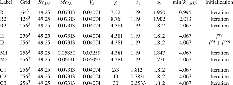
To investigate the effects of various factors on statistics, the simulations are employed with distinct parameter settings, as summarized in table 1. The influence of resolution is studied by comparing cases R1, R2 and R3 with different grids. The parameter  $s_1$ is fixed at the recommended value of
 $1.19$ proposed by Lallemand & Luo (Reference Lallemand and Luo2000), while
 $s_9$ is adjusted based on the resolution to keep the initial Taylor microscale Reynolds number the same. Besides, cases I1 and I2 utilize different initialization formulas in Appendix A to study their impact on the simulated results. Cases M1, M2 and R3 aim to explore the influence of the initial turbulent Mach number on the statistics. Here,
 $s_1$ also adopts the recommended value of
 $1.19$, and
 $s_9$ is modified to fix the initial Reynolds number at different reference temperatures. The effect of bulk-to-shear viscosity ratio on the results is studied with cases C1, C2, C3 and R3. In these cases,
 $s_1$ is modified to acquire a specific bulk-to-shear viscosity ratio, while
 $s_9$ is fixed since the reference temperature and initial Reynolds number remain constant. The same initial velocity field is applied for all cases with a resolution of
 $256^3$. And a
 $256^3$-grid resolution is chosen for the reference data acquired by the PS method, which ensures the spatial resolution
 $(k_{max}\eta ) \geqslant {\rm \pi}(1-3/N)/2.1 \approx 1.478$, as typically suggested by Pope (Reference Pope2000) for PS simulations. It is worth emphasizing that, here, the grid resolution of
 $256^3$ is adequate for resolving flow statistics at the given flow Reynolds number; however, a higher resolution may be required when exploring flow structures at higher flow Reynolds numbers or resolving solid boundaries (Falcucci et al. Reference Falcucci, Amati, Fanelli, Krastev, Polverino, Porfiri and Succi2021, Reference Falcucci, Amati, Bella, Facci, Krastev, Polverino, Succi and Porfiri2024). The main conclusions of our work remain valid for higher flow Reynolds numbers.
Parameters used in the MRT-LBE simulations.

3.2. Flow statistics associated with the velocity field
The flow statistics associated with the velocity field, including the turbulent kinetic energy, dissipation rate and velocity-derivative skewness and flatness, are discussed in this subsection. Specifically, CIOs do not appear in kinetic energy and dissipation but in higher-order statistics for velocity, including the dilatation, skewness and flatness of velocity derivatives.
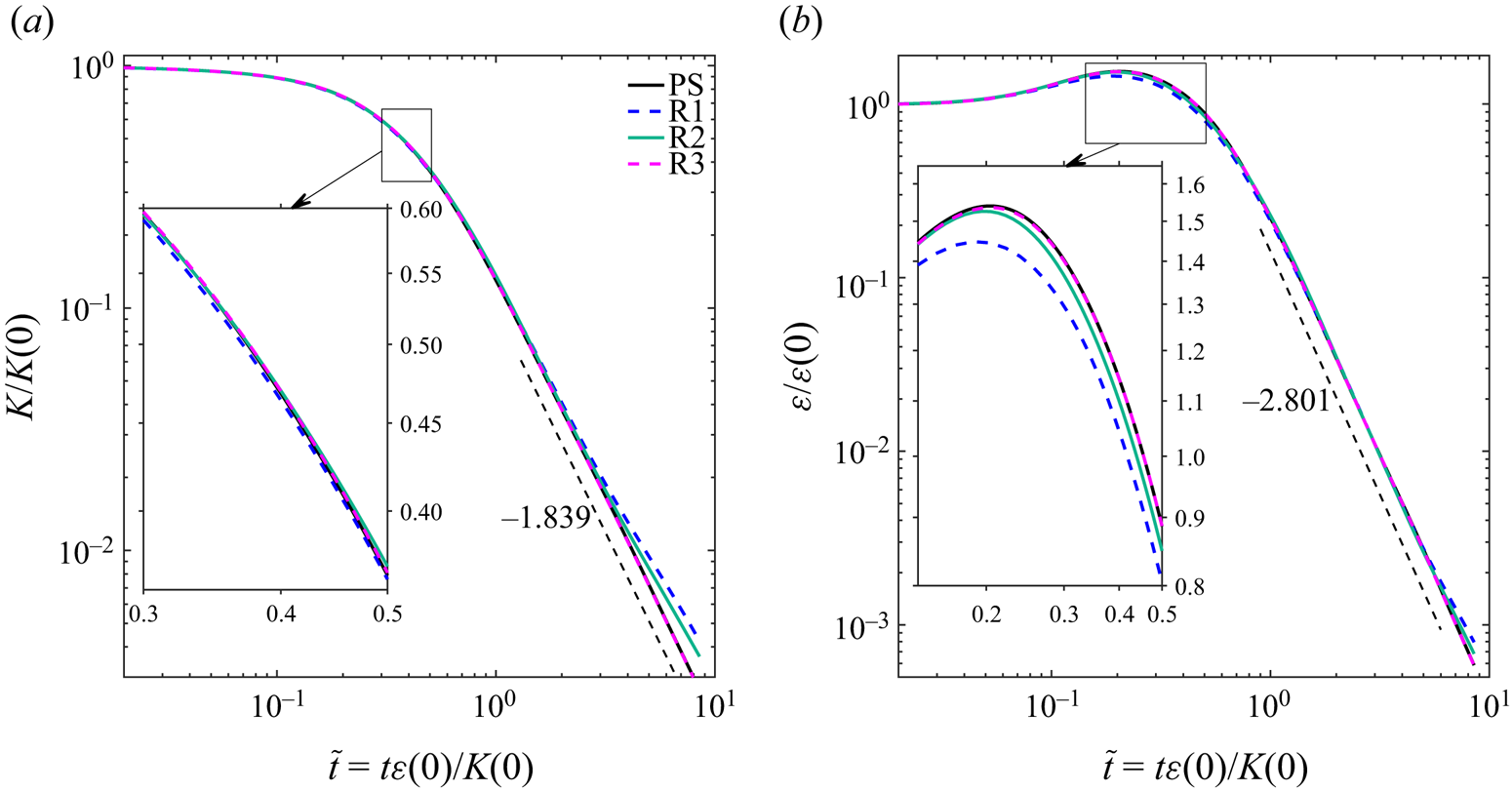
Figure 1 shows the evolutions of the turbulent kinetic energy and dissipation rate at three different grid resolutions (cases R1, R2 and R3 in table 1). In the absence of energy input, the turbulent kinetic energy decays monotonically over time, but the dissipation rate initially increases due to the development of small-scale eddies and reaches a peak at around  $0.2\sim 0.3$ dimensionless times. The results at the resolution of
 $256^3$ (case R3) agree well with the reference data obtained from the PS method, while the results at the resolutions of
 $64^3$ and
 $128^3$ appear to deviate from the PS data. The converged curves in figures 1(
 $a$) and 1(
 $b$) satisfy the scaling laws of
 $\tilde {t}^{-1.839}$ and
 $\tilde {t}^{-2.801}$, respectively, which indicates that the dissipation rate, or
 ${\rm d}K/{\rm d}t=\varepsilon$, may be used to estimate the change rate of kinetic energy in the long-term evolution. Furthermore, the results for other cases are not plotted for brevity but with the following observations: the simulation results for cases using different initialization methods, such as case I1 using only (A12a) and case I2 using both equations in (A12), are highly consistent with the reference data; the results for the cases with different initial turbulent Mach numbers (cases M1 and M2) and with different bulk-to-shear viscosity ratios (cases C1, C2 and C3), are all in good agreement with one another.
Evolutions of ( $a$) the normalized turbulent kinetic energy and (
 $b$) the normalized dissipation rate at different mesh resolutions; ‘PS’ denotes the reference data calculated by the PS method on a
 $256^3$ mesh.

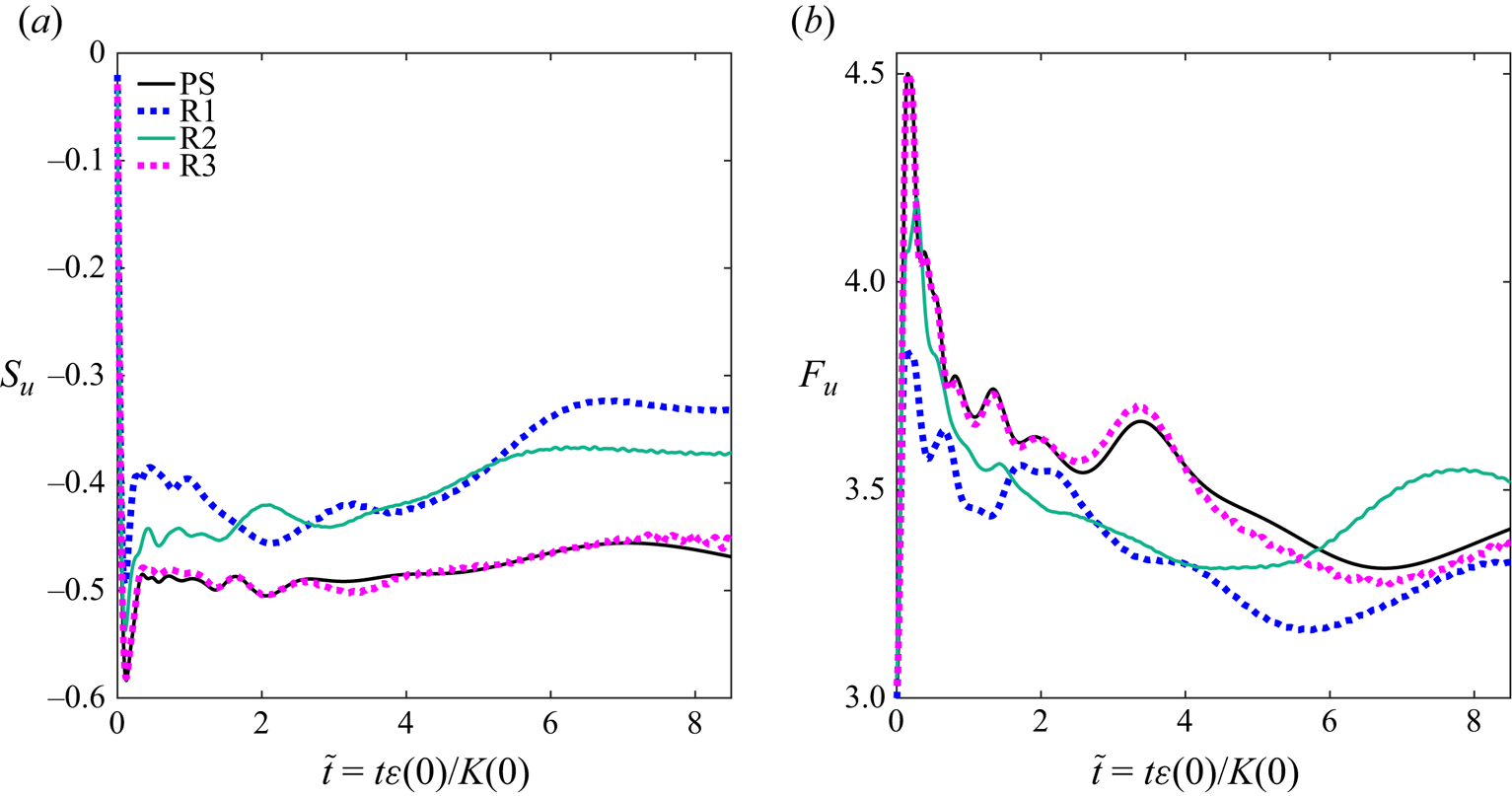
The velocity-derivative skewness is connected to vortex stretching and energy transfer among different scales, while the velocity-derivative flatness is related to internal intermittency (Pope Reference Pope2000). In order to correctly evaluate the statistics related to small scales such as the skewness and flatness shown in figure 2, the MRT-LBE method necessitates a finer resolution, namely  $(k_{max}\eta ) > 4$, compared with the PS method. This is a higher resolution requirement than what was stated in Peng et al. (Reference Peng, Liao, Luo and Wang2010), who recommended a resolution for the MRT-LBE method of
 $(k_{max}\eta ) > 2$ to resolve incompressible turbulence. Additionally, while the results for other cases are omitted here to avoid redundancy, it is worth noting that the initial Mach number and bulk-to-shear viscosity ratio, rather than different initialization methods, influence the CIOs in the skewness and flatness of the velocity derivative. Specifically, the amplitude of the CIOs decreases with decreasing initial Mach numbers or increasing bulk-to-shear viscosity ratios.
Evolutions of the velocity-derivative ( $a$) skewness and (
 $b$) flatness averaged over three directions at different mesh resolutions.

Different from the solenoidal velocity in the PS method, the velocity in the MRT-LBE method has a small but non-zero dilatation, implying that compressibility influences small-scale structures in the flow field. Figure 3 demonstrates the normalized r.m.s. dilatation for the cases in table 1. There is a significant leap in the dilatation at early times since the initial velocity is divergence free. In figure 3( $a$), the development of dilatation is suppressed as the numerical viscosity and bulk-to-shear viscosity ratio increase. In addition, figure 3(
 $b$) indicates that different initialization methods have nearly no impact on the dilatation. The Mach number mainly affects the magnitude rather than the trend of r.m.s. dilatation, while the bulk-to-shear viscosity ratio
 $\chi$ influences both trend and magnitude of r.m.s. dilatation, as shown in figures 3(
 $c$) and 3(
 $d$). A larger
 $\chi$ benefits the dampening of the r.m.s. dilatation since
 $\chi$ contributes to the diffusion term of dilatation in (2.8).
Evolutions of the normalized r.m.s. dilatation for the cases with ( $a$) different resolutions, (
 $b$) different initializations, (
 $c$) different initial turbulent Mach numbers and (
 $d$) different bulk-to-shear viscosity ratios.

Additionally, we conducted two  $512^3$ cases with
 $\chi = 0$ and
 $\chi = 15$, respectively, and compared the three-dimensional vortex structures at different times (figures omitted here for brevity). The results indicate that the compressibility effect has essentially little influence on the vortex structures at early stages, while it may suppress one or two minuscule point-like vortex structures at later stages.
3.3. Flow statistics associated with the pressure field
The CIOs are not significant in the evolution of turbulent kinetic energy and dissipation rate as the magnitude of  $\boldsymbol {u}_{C}$ is much smaller than that of
 $\boldsymbol {u}_{S}$ since
 $|\boldsymbol {u}_{C}|/|\boldsymbol {u}_{S}| \sim O(Ma)$, as shown in figure 6(
 $b$) later on. In particular, CIOs gradually emerge in pressure-related statistics with time, but they are not visible in the early stage (
 ${\tilde t} < 0.5$) of DHIT, which indicates that
 $p_{S}$ decays faster than
 $p_{C}$. In figure 4(
 $a$), the r.m.s. pressure fluctuations are jointly influenced by the varying bulk viscosity and numerical viscosity at different resolutions. When considering different initialization methods in figure 4(
 $b$), the curves of cases I1 and I2 are closer to the reference data, implying that the magnitude of the non-equilibrium distribution is significantly less than the equilibrium distribution and that the distribution function derived from the non-equilibrium distribution is more consistent with the initial hydrodynamic condition than the iterative method. As shown in figure 4(
 $c$), the r.m.s. pressure fluctuation is also impacted by the initial turbulent Mach number. And the lower the initial turbulent Mach number, the lower the CIOs in the r.m.s. pressure fluctuation. This demonstrates that, in order to eliminate CIOs and obtain a result that is more comparable to the divergence-free simulation, it is necessary to use a lower velocity scale
 $V_s$, implying more time steps and extra computational costs are needed for a simulation with the same physical time duration. Furthermore, the effects of the bulk-to-shear viscosity ratio
 $\chi$ are discussed by changing
 $s_1$. It should be emphasized that
 $\chi$ refers to a physical phenomenon and is used to describe the viscous effect triggered by the internal degrees of freedom of the gas. Here,
 $\chi$ is varied to see if the CIOs can be suppressed. Figure 4(
 $d$) illustrates that, as
 $\chi$ increases, not only are the CIOs gradually weakened, but also the r.m.s. pressure fluctuation approaches closer to the reference data.
Evolutions of the normalized r.m.s. pressure fluctuation for the cases with ( $a$) different resolutions, (
 $b$) different initializations, (
 $c$) different initial turbulent Mach numbers and (
 $d$) different bulk-to-shear viscosity ratios.

In figure 5, two pressure fluctuation spectra, corresponding to the early and fully developed stages of the flow field for the moments  $\tilde {t}=t\varepsilon (0)/K(0)=0.4258$ (
 $t=1$) and
 $\tilde {t}=t\varepsilon (0)/K(0)=2.129$ (
 $t=5$), respectively, are presented for the cases with different initial turbulent Mach numbers and bulk-to-shear viscosity ratios. To maintain brevity, the results of other cases are skipped, but the observations are noteworthy: the initialization method does not obviously affect the spectra, and the differences for different cases occur in the pressure fluctuation spectra rather than the kinetic energy and dissipation spectra. Specifically, deviations from reference data are observed in the pressure fluctuation spectra at both low- and high-wavenumber ranges, which might result from CIOs and numerical errors in the MRT-LBE method. A comparison of pressure fluctuation spectra at different times reveals minor differences in the high-wavenumber range, but the differences in the low-wavenumber range increase over time. The deviations observed in the low-wavenumber range might correlate with the different magnitudes of CIOs in each case, indicating that the pressure-related statistics in the low-wavenumber range are primarily contaminated by CIOs. Finally, it should be pointed out that
 $\chi$ modulates the low-wavenumber parts of the pressure fluctuation spectra, bringing the curve closer to the reference data.
The pressure fluctuation spectra  $\delta P(k,t)$ with the resolution of
 $256^3$ at (
 $a$)
 $\tilde {t}=t\varepsilon (0)/K(0)=0.4258$ (
 $t=1$) and (
 $b$)
 $\tilde {t}=t\varepsilon (0)/K(0)=2.129$ (
 $t=5$).

It is important to emphasize that raising  $\chi$ has the same effect as raising the total viscosity (the sum of shear and bulk viscosity) at a given shear viscosity, which is typically believed to improve numerical stability. However, our code blows up when
 $\chi =100$ (
 $s_1 = 0.1209$), so a very large
 $\chi$ can cause numerical instability. The linear instability analysis (Lallemand & Luo Reference Lallemand and Luo2000) revealed that a large
 $\chi$ means a small
 $s_1$, violating the rule of thumb that
 $s_1$ is recommended to be greater than
 $0.5$ and resulting in numerical instability. Therefore, to suppress CIOs and improve the validity of the results from the MRT-LBE method,
 $s_1$ should be adjusted to be as small as is feasible for a large
 $\chi$, provided that the numerical stability is maintained.
4. Analysis of the flow field based on the Helmholtz–Hodge decomposition
To examine the validity of the magnitude relationship utilized in asymptotic analysis and better understand the underlying origin of CIOs, the Helmholtz–Hodge decomposition (Wu et al. Reference Wu, Ma and Zhou2015), which provides a unique decomposition of a vector field into its divergence-free and curl-free components, is applied to meticulously analyse the flow fields of all cases presented in table 1. In general, the divergence-free velocity projection procedure (Patankar Reference Patankar1980) may be applied to decompose the solenoid and compressive components of the flow field when wall boundaries are present. Specifically, for periodic boundary conditions, the velocity can be decomposed into a solenoidal component and a compressive component in spectral space, namely,
 \begin{equation} \hat{\boldsymbol{u}}_S (\boldsymbol{k},t) = \hat{\boldsymbol{u}} (\boldsymbol{k},t) - \frac{ \hat{\boldsymbol{u}} (\boldsymbol{k},t) \boldsymbol{\cdot} \boldsymbol{k} }{k^2} \boldsymbol{k},\quad \hat{\boldsymbol{u}}_C (\boldsymbol{k},t) = \frac{ \hat{\boldsymbol{u}} (\boldsymbol{k},t) \boldsymbol{\cdot} \boldsymbol{k} }{k^2} \boldsymbol{k}, \end{equation}
where  $\widehat { ( \cdots ) }$ denotes the converted physical variable in the
 $\boldsymbol {k}$ spectral space and each component of the wavenumber vector
 $\boldsymbol {k}=(k_x,k_y,k_z)$ ranges from
 $1-N/2$ to
 $N/2$ depending on the grid resolution
 $N$. The solenoidal and compressive pressure can be evaluated by
 \begin{equation} \widehat{ p_S } ={-} \rho_0 \frac{ {\rm i} \boldsymbol{k} }{k^2} \boldsymbol{\cdot} \widehat{ \left( \boldsymbol{u}_S\times\boldsymbol{\omega}_S \right) } - \rho_0 \widehat{ \left( \frac{u_S^2 }{2} \right) } ,\quad p_C = c_s^2 \delta \rho - p_S , \end{equation}
where  ${\rm i} \equiv \sqrt {-1}$.
Figures 6( $a$) and 6(
 $b$) clearly demonstrate the evolution of the amplitude relationships pertaining to the r.m.s. values of density and velocity components, respectively. Consequently, the magnitude assumptions between solenoidal and compressional components in (2.5a,b) are validated, confirming that the corresponding results of asymptotic analysis are applicable to DHIT. Specifically, figure 6(
 $c$) confirms that
 $p_{S}$ decays faster than
 $p_{C}$, which explains why CIOs emerge and contaminate the simulated results over time, and the ratio between the moduli for different pressure gradients in figure 6(
 $d$) reveals that the compressive pressure affects the flow field along with the solenoidal pressure over time. Furthermore, different cases imply that the ratios of the compressive components
 $u_{C,rms}$ and
 $p_{C,rms}$ in the flow can be reduced by augmenting the bulk-to-shear viscosity ratio or decreasing the initial turbulent Mach number, providing us with a method to suppress the CIOs in the pressure-related statistics.
Evolutions of the magnitude relationships for ( $a$) the density, (
 $b$) velocity, (
 $c$) pressure and (
 $d$) the ratio between the moduli for different pressure gradients in the MRT-LBE method.

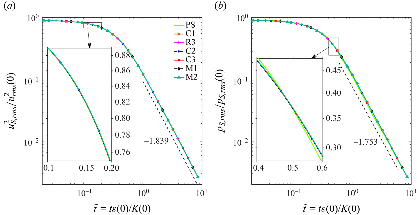
The evolution of r.m.s. solenoidal velocity and pressure for the MRT-LBE method is shown in figure 7. Several observations can be made. First, in all cases, the results are essentially identical and are in excellent agreement with the PS method, showing that, in the case of DHIT in a periodic domain, the solenoidal components can in fact be precisely recovered when the compressive components are removed, and both  $\boldsymbol {u}_S$ and
 $p_S$ are independent of the numerical Mach number and bulk-to-shear viscosity ratio. Figure 7(
 $a$) depicts the evolution of the mean-square solenoidal velocity, which yields a long-term scaling behaviour
 $\tilde {t}^{-1.839}$. It is noteworthy that this slope is identical to the slope
 $\tilde {t}^{-1.839}$ in figure 1(
 $a$), indicating that the compressive velocity has little effect on the turbulent kinetic energy in the MRT-LBE method. The solenoidal components in the MRT-LBE approach are accurate and noise free, as the solenoidal pressure solely depends on the solenoidal velocity. Note that the initial values
 $u_{rms}(0) = 1.036$ and
 $p_{S, rms}(0) = 1.153$ in spectral-simulation units, combined with the two plots in figure 7, confirm that the scaling relation
 $p_{S,rms}\sim \rho _0 u_{rms}^2$ holds. The above results indicate that the underlying causes of CIOs are
 $\boldsymbol {u}_{C}$ and
 $p_{C}$, which result from the compressibility inherent in the MRT-LBE method.
Evolutions of ( $a$) the normalized r.m.s. solenoidal velocity and (
 $b$) the normalized r.m.s. solenoidal pressure calculated from the solenoidal velocity where
 $u_{rms}(0) = 1.036$ and
 $p_{S,rms}(0) = 1.153$, both in spectral-simulation units, on a
 $256^3$ mesh.

The CIO period is comparable to the sound wave propagation time scale and is much shorter than the typical advection time scale in the NS equations. When sound waves propagate in a periodic cube, their characteristic time may be written as  $L V_s/c_s$ in spectral units, and their dimensionless characteristic time is
 $L V_s\varepsilon (0)/(c_s K(0))$. The dimensionless average periods of CIOs obtained from the r.m.s. pressure fluctuation are listed in table 2, which are approximately half of the dimensionless characteristic time
 $L V_s\varepsilon (0)/(c_s K(0))$, confirming the acoustics-like behaviour of the CIOs.
Average periods of the CIOs in the normalized r.m.s. pressure fluctuation for different cases.

5. Analysis of the evolution of the mean-square pressure fluctuations
5.1. Analysis of different terms in the evolution equation
Here, a quantitative model is developed to describe the evolution of the mean-square pressure fluctuation in the MRT-LBE method. The evolution and magnitude of each term in (2.12) are carefully analysed for different cases, and the result of case C3 is plotted in figure 8, for instance. In particular, the magnitudes of term  $B$ and term
 $C$ are similar and significantly larger than the other components, suggesting that the coupling effect of the density and compressive-pressure gradients along with the dilatation effect are responsible for the majority of the pressure fluctuations. The magnitude of
 $F$ increases gradually until it becomes comparable to the magnitudes of term
 $B$ and term
 $C$ as the bulk-to-shear viscosity ratio rises, as seen in figure 8(
 $b$). The magnitudes of
 $A$,
 $D$ and
 $E$ are relatively small, indicating that the coupling effects arising from the interaction of vorticity and density fluctuations, the density and solenoidal-pressure gradients, as well as the viscous dissipation induced by solenoidal strain and density gradient, primarily contribute to the local high-frequency oscillations in CIOs. These effects, despite their limited scope, are relevant to the effects of pressure fluctuations on the fine structure of the flow field in the MRT-LBE method. Consequently, when considering the long-term evolution of pressure in the flow field,
 $B$,
 $C$ and
 $F$ are paramount and need to be meticulously modelled, while
 $A$,
 $D$ and
 $E$, which only contribute primarily to finite, high-frequency oscillations, can be deemed negligible for the purposes of analysis.
Evolutions of ( $a$) the terms and (
 $b$) their absolute values in (2.12) for case C3.

The long-term evolutions of terms  $B$,
 $C$ and
 $F$ are plotted in figure 9 using the appropriate scales on the horizontal and vertical axes. At a given initial Taylor microscale Reynolds number, both terms
 $B$ and
 $C$ decay exponentially at the same rate. It is noted that terms
 $B$ and
 $C$ in case C3 decay quickly compared with the other cases, because the bulk viscosity suppresses the dilatation or compressive pressure, as shown in (2.7a) and (2.8). However, it should be noted that, while increasing the bulk-to-shear viscosity ratio inhibits dilatation, it does not necessarily weaken the coupling term between the bulk-to-shear viscosity ratio and dilatation, i.e. the magnitude of term
 $F$ may even increase, as shown in figure 9(
 $c$).
Evolutions of term ( $a$)
 $B$, term (
 $b$)
 $C$, term (
 $c$)
 $F$ and (
 $d$) the sum of other terms in (2.10) for different cases.

The numerical results imply that the sum of  $B$ and
 $C$ at long times can be quantitatively expressed as
 \begin{equation} B+C = \rho_{0}\langle\vartheta^2\rangle - \frac{ 1}{\rho_0 } \left\langle \boldsymbol{\nabla}\delta\rho \boldsymbol{\cdot} \boldsymbol{\nabla} p_C \right\rangle = C_1 \exp{( - C_2 \tilde{t} )} , \end{equation}
where  $C_1$ is related to the bulk-to-shear viscosity ratio and initial turbulent Mach number, and
 $C_2$ is an undetermined coefficient that is only related to the bulk-to-shear viscosity ratio. On the other hand,
 $F$ appears to follow a power law, which is approximated by
 \begin{equation} F = \nu \left( \chi + \tfrac{4 }{3} \right) \left\langle \boldsymbol{\nabla}\delta\rho \boldsymbol{\cdot}\boldsymbol{\nabla}\vartheta \right\rangle = \nu \left( \chi + \tfrac{4 }{3} \right) C_{3} \tilde{t}^{ {-}C_{4} } , \end{equation}
where  $C_3$ is only connected to the initial turbulent Mach number and
 $C_4$ is fixed for the case with the same initial Taylor microscale Reynolds number. By combining the aforementioned formulas, (2.12) changes to the following second-order ordinary differential equation:
 \begin{equation} \frac{{\rm d}^2}{{\rm
d}t^2} [ \left(\delta p\right)_{rms}^2 ] =
\left( \frac{\varepsilon(0)}{K(0)} \right)^2 \frac{{\rm
d}^2}{{\rm d}\tilde{t}^2} \langle \delta p^2
\rangle \approx 2\rho_0 c_s^4 \left[ C_1 {\rm e}^{ -
C_2 \tilde{t} } + \nu \left( \chi + \frac{4 }{3} \right)
C_{3} \tilde{t}^{{-}C_{4}} \right] ,
\end{equation}
and the solution is
 \begin{align} \left(\delta
p\right)_{rms}^2 = \langle \delta p^2 \rangle
\approx 2\rho_0 c_S^4 \left( \frac{K(0)}{\varepsilon(0)}
\right)^2 \left[ \frac{ C_1 }{C_2^2 } {\rm e}^{ - C_2
\tilde{t} } + \frac{ \nu \left( \chi + {4 / 3} \right)
C_{3}}{( C_4 - 1 ) ( C_4 - 2 ) } \tilde{t}^{ {-}C_4 + 2 } +
C_5 \tilde{t} + C_6 \right] ,
\end{align}
where  $C_5$ and
 $C_6$ must be equal to zero as the mean-square pressure fluctuations go to zero when
 ${\tilde t}\to \infty$.
5.2. Comparison of the model with simulation results
The quantitative model in (5.4) is applied for the cases in table 1. With  $C_2 = 0.02064 \chi + 0.1483$ and
 $C_4 = 5.617$ for the initial Taylor microscale Reynolds number
 $Re_{\lambda,0} = 49.25$, the mean-square pressure fluctuation is approximated by
 \begin{align} \left(\delta p\right)_{rms}^2 \approx 2\rho_0 c_S^4 \left( \frac{K(0)}{\varepsilon(0)} \right)^2 \left\{ \frac{ C_1 \exp({ - ( 0.02064 \chi + 0.1483 ) \tilde{t}}) }{\left( 0.02064 \chi + 0.1483 \right)^2 } + \nu \left( \chi + \frac{4}{3} \right) \frac{C_{3}}{16.70 } \tilde{t}^{{-}3.617 } \right\}, \end{align}
where  $C_1$ is determined by both the bulk-to-shear viscosity ratio and the initial turbulent Mach number, and
 $C_3$ depends on the initial turbulent Mach numbers.
To assess the accuracy of the quantitative model, the simulation results and the mean-square pressure fluctuations predicted by (5.5) are concurrently plotted in figure 10. Equation (5.5) accurately captures the long-term average behaviour of the mean-square pressure fluctuations, but it is not designed to predict the oscillations at the acoustic time scale. The success of the model indicates the usefulness of the derived evolution (2.12) for studying the CIOs in the MRT-LBM method. Moreover, further augmentation of the bulk viscosity leads to a significant increase in the magnitude of  $F$ in (2.12), which diminishes the contributions of terms
 $B$ and
 $C$. Consequently, the linear superposition of terms
 $B$,
 $C$ and
 $F$ upon which (5.5) relies ceases to be appropriate as the bulk-to-shear viscosity ratio
 $\chi$ rises. When
 $\chi$ is substantial, considering solely
 $F$, the resulting mean-square pressure fluctuations adhere to a power law of
 $\tilde {t}^{ -3.617 }$, which closely matches the power law of
 $\tilde {t}^{ -3.505 }$ obtained by the incompressible PS method. Therefore, based on the power law behaviour of
 $F$ in (5.5), it can be argued that a large
 $\chi$ effectively enhances the prediction of statistical quantities, particularly the r.m.s. pressure, within the flow field of the MRT-LBE method. In other words, a large
 $\chi$ does not affect the solenoidal component of the flow.
Evolutions of the mean-square pressure fluctuations and their long-term approximations obtained by (5.5) for different cases.

6. Summary and conclusions
In general, CIOs can significantly impact the statistical quantities of simulated turbulent flows in artificial compressibility methods, no matter whether the method is based on the macroscopic NS equations or the kinetic model Boltzmann equation. In particular, CIOs result in inaccuracies in the long-term prediction of r.m.s. pressure fluctuations. The current study intends to provide a deep understanding of the CIOs within the MRT-LBE method, from both theoretical and numerical perspectives.
On the theoretical front, the incompressible NS equations governing  $\boldsymbol {u}_{S}$ and the governing equations for the compressible velocity component
 $\boldsymbol {u}_{C}$ have been derived using the asymptotic analysis based on the Mach number proposed by Majda (Reference Majda1984). It is important to note that, in artificial compressibility methods, the Mach number is a numerical parameter, and for computational efficiency, the numerical Mach number is typically set to a finite value of
 ${O}(0.1)$. In particular, the evolution of
 $\boldsymbol {u}_{S}$ is independent of
 $\boldsymbol {u}_{C}$ and
 $\delta \rho$, but the evolution of
 $\boldsymbol {u}_{C}$ is coupled with
 $\boldsymbol {u}_{S}$ and
 $\delta \rho$. This analysis yields an evolution equation of the mean-square pressure fluctuation which reveals several coupling effects, including the couplings of density fluctuations with vorticity, solenoidal strain and the solenoidal- and compressive-pressure fields, as well as several dissipation mechanisms, including one associated with the bulk-to-shear viscosity ratio.
With the Helmholtz–Hodge decomposition, a detailed and comprehensive analysis of the solenoidal and compressive components of the flow field obtained from the MRT-LBE method has been conducted, revealing that the ratio of compressive velocity and solenoidal velocity is indeed approximately  $O(Ma^2)$, as expected for a physically weakly compressible flow. Compared with the PS method, the solenoidal components obtained from the MRT-LBE method are accurate, while the compressive components are identified as the primary source for CIOs.
Numerical simulations of DHIT at  $Re_{\lambda,0} = 49.25$ have been conducted to explore the effects of various factors on statistical quantities and spectra of a turbulent flow. The results indicate that the CIOs gradually weaken as the initial turbulent Mach number decreases and the bulk-to-shear viscosity ratio
 $\chi$ increases. To reduce the CIOs in the statistics, which are mainly caused by the compressive pressure
 $p_C$, the compressive component of pressure in the MRT-LBE method needs to be suppressed. We propose that increasing the bulk-to-shear viscosity ratio
 $\chi$ is an effective method to correct the pressure. The accuracy and reliability of the simulations are increased by this procedure, which maintains the general trends of the flow statistics while also bringing the simulated results of the MRT-LBE method closer to those of the PS method. Additional simulations had been performed with initial Taylor microscale Reynolds numbers
 $Re_{\lambda,0}$ of
 $39.40$ and
 $59.07$ (not shown here for brevity); and these simulations validate our proposed model for the mean-square pressure fluctuation and also illustrate the effectiveness of increasing bulk-to-shear viscosity ratios for reducing CIOs in pressure-related statistics.
Based on the evolution equation of the pressure fluctuation, a model is developed for the pressure fluctuation, which successfully predicts the time evolution of r.m.s. pressure fluctuation in DHIT. This model clarifies that bulk viscosity suppresses CIOs in pressure by enhancing the viscous dissipation caused by dilatation and density gradients. Given that this model is derived from the weakly compressible NS equations, it not only enhances our understanding of pressure evolution within the MRT-LBE method but also provides a better comprehension of CIOs in other artificial compressibility methods and weakly compressible flows.
Funding
Y.Q. thanks J. Shen for many useful discussions. This work has been supported by the National Natural Science Foundation of China (NSFC award numbers T2250710183, U2241269, 91852205, 11961131006), NSFC Basic Science Center Program (award number 11988102), the Taizhou-Shenzhen Innovation Center, Guangdong Provincial Key Laboratory of Turbulence Research and Applications (2023B1212060001), Guangdong-Hong Kong-Macao Joint Laboratory for Data-Driven Fluid Mechanics and Engineering Applications (2020B1212030001) and Shenzhen Science & Technology Program (grant no. KQTD20180411143441009, 2020-148). Computing resources are provided by the Center for Computational Science and Engineering of Southern University of Science and Technology.
Declaration of interests
The authors report no conflict of interest.
Data availability statement
The data that support the findings of this study are available from the corresponding author upon reasonable request.
Appendix A. The three-dimensional MRT-LBE method
The evolution equation of the MRT-LBE method (d'Humieères et al. Reference d'Humieères, Ginzburg, Krafczyk, Lallemand and Luo2002) for nearly incompressible flows is
 \begin{equation} \boldsymbol{f}\left(\boldsymbol{x} + \boldsymbol{\xi}_\alpha \Delta t, t + \Delta t\right) - \boldsymbol{f}\left(\boldsymbol{x}, t\right) ={-} \boldsymbol{M}^{{-}1}\boldsymbol{\cdot}\boldsymbol{S}\boldsymbol{\cdot}\left[ \boldsymbol{m}\left(\boldsymbol{x}, t\right) - \boldsymbol{m}^{eq}\left(\boldsymbol{x}, t\right) \right] , \end{equation}
where  $\boldsymbol {M}$ is an orthogonal transformation matrix and
 $\boldsymbol {S}$ is the collision relaxation matrix. The distribution function
 $\boldsymbol {f}$ and the moment
 $\boldsymbol {m}$ with the D3Q19 discrete velocity model
 $\boldsymbol {\xi }_\alpha$ are expressed explicitly as
 $$\begin{gather} \boldsymbol{f}\left(\boldsymbol{x}, t\right) = f_\alpha\left(\boldsymbol{x}, t\right) = \left(\, f_{0}\left(\boldsymbol{x}, t \right), f_{1}\left(\boldsymbol{x}, t \right), \ldots, f_{18}\left(\boldsymbol{x} , t \right) \right)^{\rm T} , \end{gather}$$
 $$\begin{gather}f_\alpha \left(\boldsymbol{x} + \boldsymbol{\xi}_\alpha \Delta t, t + \Delta t\right) = \left(\, f_{0}\left(\boldsymbol{x} + \boldsymbol{\xi}_{0}\Delta t, t + \Delta t\right), \ldots, f_{18}\left(\boldsymbol{x} + \boldsymbol{\xi}_{18}\Delta t, t + \Delta t\right) \right)^{\rm T}, \end{gather}$$
 $$\begin{gather}\boldsymbol{m}(\boldsymbol{x}, t) = m_\alpha\left(\boldsymbol{x}, t\right) = \left( m_{0}(\boldsymbol{x}, t), m_{1}(\boldsymbol{x}, t), \ldots, m_{18}(\boldsymbol{x}, t) \right)^{\rm T}, \end{gather}$$
 $$\begin{gather}\boldsymbol{m}^{eq}(\boldsymbol{x}, t) = m_\alpha^{eq} \left(\boldsymbol{x}, t\right) = \left( m_{0}^{eq}(\boldsymbol{x}, t), m_{1}^{eq}(\boldsymbol{x}, t), \ldots, m_{18}^{eq}(\boldsymbol{x}, t) \right)^{\rm T} . \end{gather}$$
The key concept of MRT-LBE is that the streaming substep is handled by the on-lattice discrete velocity model, while the collision substep is performed in the physical moment space. The transformation matrix  $\boldsymbol {M}$ is applied to convert the distribution function
 $\boldsymbol {f}$ in the discrete particle velocity space
 $\boldsymbol {\xi }_\alpha$ to the moment space
 $\boldsymbol {m}$ by
 \begin{equation} \boldsymbol{m}=\boldsymbol{M}\boldsymbol{\cdot}\boldsymbol{f} , \quad \boldsymbol{f}=\boldsymbol{M}^{{-}1}\boldsymbol{\cdot}\boldsymbol{m} . \end{equation}
For the D3Q19 model (d'Humieères et al. Reference d'Humieères, Ginzburg, Krafczyk, Lallemand and Luo2002), the nineteen discrete velocities are
 \begin{align} \boldsymbol{\xi}_\alpha
= \left\{\!\! \begin{array}{@{}ll} ( 0, 0, 0 ), & \alpha = 0 ,
\\ ({\pm}\sqrt{3}, 0, 0 )c_s, ( 0, \pm\sqrt{3}, 0 )c_s, (
0, 0, \pm\sqrt{3} )c_s, & \alpha = 1 \sim 6 , \\
({\pm}\sqrt{3}, \pm\sqrt{3}, 0 )c_s, ({\pm}\sqrt{3}, 0,
\pm\sqrt{3})c_s, ( 0, \pm\sqrt{3}, \pm\sqrt{3})c_s, &
\alpha = 7 \sim 18 , \end{array} \right.
\end{align}
where  $c_s = \sqrt {RT}$ is the fixed sound of speed with a prescribed specific gas constant
 $R$ and a fixed temperature
 $T$ for athermal flows.
The macroscopic hydrodynamic variables, including the density  $\rho$ and the velocity
 $\boldsymbol {u}$, are obtained from the moments of the distribution function
 $\boldsymbol {f}$ for the nearly incompressible approximation (He & Luo Reference He and Luo1997) as the following:
 \begin{equation} \rho = \rho_0 + \delta \rho , \quad\rho_0 = 1 ;\quad\delta \rho = \sum_{ \alpha } f_\alpha , \quad\rho_0 \boldsymbol{u} = \sum_{ \alpha } \boldsymbol{\xi}_\alpha f_\alpha , \end{equation}
where  $\rho _0$ is the mean density, and
 $\delta \rho$ is the density fluctuation assumed to be
 $|\delta \rho |\ll \rho _0$. The corresponding nineteen orthogonal moments
 \begin{equation} \boldsymbol{m} = m_\alpha = \left( \delta\rho, e, \epsilon, j_x, q_x, j_y, q_y, j_z, q_z, 3p_{xx}, 3{\rm \pi}_{xx}, p_{ww}, {\rm \pi}_{ww}, p_{xy}, p_{yz}, p_{xz}, m_{x}, m_{y}, m_{z} \right)^{\rm T}, \end{equation}
are defined through the element of the transformation matrix  $\boldsymbol {M}$ as
 $$\begin{gather} M_{0,\alpha} = |\boldsymbol{\xi}_\alpha|^0 = 1, \quad M_{1,\alpha} = 19|\boldsymbol{\xi}_\alpha|^2 - 30, \quad M_{2,\alpha} = \left( 21|\boldsymbol{\xi}_\alpha|^4 - 53|\boldsymbol{\xi}_\alpha|^2 + 24 \right)/2 , \end{gather}$$
 $$\begin{gather}M_{3,\alpha} = \xi_{\alpha x}, \quad M_{4,\alpha} = \left( 5|\boldsymbol{\xi}_\alpha|^2 - 9 \right) \xi_{\alpha x}, \quad M_{5,\alpha} = \xi_{\alpha y}, \end{gather}$$
 $$\begin{gather}M_{6,\alpha} = \left( 5|\boldsymbol{\xi}_\alpha|^2 - 9 \right) \xi_{\alpha y}, \quad M_{7,\alpha} = \xi_{\alpha z}, \quad M_{8,\alpha} = \left( 5|\boldsymbol{\xi}_\alpha|^2 - 9 \right) \xi_{\alpha z}, \end{gather}$$
 $$\begin{gather}M_{9,\alpha} = 3 \xi_{\alpha x}^2 - |\boldsymbol{\xi}_\alpha|^2, \quad M_{10,\alpha} = \left( 3 |\boldsymbol{\xi}_\alpha|^2 - 5 \right)\left( 3 \xi_{\alpha x}^2 - |\boldsymbol{\xi}_\alpha|^2 \right) , \end{gather}$$
 $$\begin{gather}M_{11,\alpha} = \xi_{\alpha y}^2 - \xi_{\alpha z}^2, \quad M_{12,\alpha} = \left( 3 |\boldsymbol{\xi}_\alpha|^2 - 5 \right)\left( \xi_{\alpha y}^2 - \xi_{\alpha z}^2 \right) ,\quad M_{13,\alpha} = \xi_{\alpha x} \xi_{\alpha y}, \end{gather}$$
 $$\begin{gather}M_{14,\alpha} = \xi_{\alpha y} \xi_{\alpha z}, \quad M_{15,\alpha} = \xi_{\alpha x} \xi_{\alpha z} , \quad M_{16,\alpha} = \left( \xi_{\alpha y}^2 - \xi_{\alpha z}^2 \right)\xi_{\alpha x} , \end{gather}$$
 $$\begin{gather}M_{17,\alpha} = \left( \xi_{\alpha z}^2 - \xi_{\alpha x}^2 \right)\xi_{\alpha y} , \quad M_{18,\alpha} = \left( \xi_{\alpha x}^2 - \xi_{\alpha y}^2 \right)\xi_{\alpha z} , \end{gather}$$
with the equilibrium moments given as
 $$\begin{gather} \delta\rho^{eq} = \delta\rho, \quad e^{eq} ={-}11\delta\rho + \frac{19}{\rho_0}\left( j_x^2 + j_y^2 + j_z^2 \right), \quad \epsilon^{eq} = w_\epsilon \delta\rho + \frac{w_{\epsilon j} }{\rho_0}\left( j_x^2 + j_y^2 + j_z^2 \right) , \end{gather}$$
 $$\begin{gather}j_x^{eq} = j_x = \rho_0 u_x, \quad q_x^{eq} ={-}\tfrac{2}{3}j_x, \quad j_y^{eq} = j_y = \rho_0 u_y,\quad q_y^{eq} ={-}\tfrac{2}{3}j_y, \quad j_z^{eq} = j_z = \rho_0 u_z, \end{gather}$$
 $$\begin{gather}q_z^{eq} ={-}\frac{2}{3}j_z, \quad p_{xx}^{eq} = \frac{1}{3\rho_0}\left( 2j_x^2 - j_y^2 - j_z^2 \right), \quad {\rm \pi}_{xx}^{eq} = w_{xx} p^{eq}_{xx} , \quad p_{ww}^{eq} = \frac{1}{\rho_0}\left( j_y^2 - j_z^2 \right), \end{gather}$$
 $$\begin{gather}{\rm \pi}_{ww}^{eq} = w_{xx} {\rm \pi}^{eq}_{xx} , \quad p_{xy}^{eq} = \frac{j_x j_y}{\rho_0}, \quad p_{yz}^{eq} = \frac{j_y j_z}{\rho_0}, \quad p_{xz}^{eq} = \frac{j_x j_z}{\rho_0}, \quad m^{eq}_{x} = m^{eq}_{y} = m^{eq}_{z} = 0 , \end{gather}$$
where the coefficients  $w_\epsilon$,
 $w_{\epsilon j}$ and
 $w_{xx}$ are free parameters in the D3Q19 model. The diagonal matrix
 $\boldsymbol {S}$ specifies the positive relaxation rates, which must satisfy the stability condition
 $s_\alpha >1/2$, (Lallemand & Luo Reference Lallemand and Luo2000; d'Humieères et al. Reference d'Humieères, Ginzburg, Krafczyk, Lallemand and Luo2002; Lallemand & Luo Reference Lallemand and Luo2003) for all non-conserved moments, as follows:
 \begin{equation} \boldsymbol{S} = {\rm diag}\left( 0, s_{1}, s_{2}, 0, s_{4}, 0, s_{4}, 0, s_{4}, s_{9}, s_{10}, s_{9}, s_{10}, s_{13}, s_{13}, s_{13}, s_{16}, s_{16}, s_{16} \right) . \end{equation}
The kinematic viscosity  $\nu$ and the bulk viscosity
 $\xi$ are determined by the relaxation parameters
 $s_{9}$ and
 $s_{1}$, respectively,
 $$\begin{gather} \nu = \frac{1}{\sqrt{3}}\left( \frac{1}{s_9} - \frac{1}{2} \right) c_s \Delta x , \end{gather}$$
 $$\begin{gather}\zeta = \frac{5 - 9c_s^2}{3\sqrt{3}}\left( \frac{1}{s_1} - \frac{1}{2} \right) c_s \Delta x , \end{gather}$$
where  $\Delta x$ is the grid spacing, and the bulk-to-shear viscosity ratio can be calculated as
 $\chi = \zeta / \nu$. In the simulations, we use some of the suggested parameters
 $w_\epsilon =0$,
 $w_{\epsilon j}=-475/63$,
 $w_{xx}=0$,
 $s_1=1.19$,
 $s_2=s_{10}=1.4$,
 $s_4=1.2$ and
 $s_{16}=1.98$ consistent with Lallemand and Luo's linear analysis (Lallemand & Luo Reference Lallemand and Luo2000) to maximize the stability of the model, while leaving
 $s_9=s_{13}$ as a free parameter to change the kinematic shear viscosity
 $\nu$. Additionally, for situations with varying bulk-to-shear viscosity ratios
 $\chi$, both
 $s_1$ and
 $s_9$ are altered.
By using the Chapman–Enskog analysis, He & Luo (Reference He and Luo1997) proved that the incompressible approximation, which is used in the MRT-LBE method, recovers the weakly compressible NS equations (2.1), up to the order of  $O(Ma^2)$, and recovering the weakly compressible NS equations requires the following velocity moments:
 $$\begin{gather} \sum_{ \alpha } f_\alpha^{eq} = \delta \rho , \quad \sum_{ \alpha } \boldsymbol{\xi}_\alpha\, f_\alpha^{eq} = \rho_0 \boldsymbol{u} , \quad \sum_{ \alpha } \boldsymbol{\xi}_\alpha \boldsymbol{\xi}_\alpha\, f_\alpha^{eq} = \rho_0 \left( \boldsymbol{u} \boldsymbol{u} + c_s^2\boldsymbol{I} \right) , \end{gather}$$
 $$\begin{gather}\sum_{ \alpha } f_\alpha^{neq} = 0 , \quad \sum_{ \alpha } \boldsymbol{\xi}_\alpha\, f_\alpha^{neq} = \boldsymbol{0}, \quad \left(1 - {s_9\over 2} \right) \sum_{ \alpha } \boldsymbol{\xi}_\alpha \boldsymbol{\xi}_\alpha\, f_\alpha^{neq} ={-} \boldsymbol{\sigma} , \end{gather}$$
where  $\boldsymbol {f}^{eq}$ is the equilibrium part and
 $\boldsymbol {f}^{neq}$ is the non-equilibrium part of the distribution function
 $\boldsymbol {f}=\boldsymbol {f}^{eq}+\boldsymbol {f}^{neq}$. For simplicity, all the unmentioned moments can be set to zero for the Hermite expansions of
 $f_\alpha ^{eq}$ and
 $f_\alpha ^{neq}$, and the truncated Hermite polynomial expansions (see Appendix D) are constructed from the above moments, giving
 $$\begin{gather} f_\alpha^{eq,(2)} = w_\alpha \left\{ \delta\rho + \rho_0 \left[ \frac{ \boldsymbol{u} \boldsymbol{\cdot} \boldsymbol{\xi}_\alpha }{ c_s^2 }+ \frac{1}{2}\left( \frac{ \boldsymbol{u} \boldsymbol{\cdot} \boldsymbol{\xi}_\alpha }{ c_s^2 } \right)^2 - \frac{ u^2 }{ 2 c_s^2 } \right] \right\} , \end{gather}$$
 $$\begin{gather}f_\alpha^{neq,(2)} = {2 \over 2 - s_9} w_\alpha \frac{\rho_0 \nu }{c_s^2} \left( \vartheta - \frac{ \boldsymbol{\xi}_\alpha \boldsymbol{\cdot} \boldsymbol{S} \boldsymbol{\cdot} \boldsymbol{\xi}_\alpha }{ c_s^2 } \right) , \end{gather}$$
where  $f_\alpha ^{eq,(2)}$ and
 $f_\alpha ^{neq,(2)}$ represent the second-order Hermite expansion of
 $\boldsymbol {f}^{eq}$ and the second-order Hermite expansion of
 $\boldsymbol {f}^{neq}$, respectively, and
 $w_\alpha$ is the corresponding weights of the D3Q19 velocity model (Qian et al. Reference Qian, d'Humieères and Lallemand1992). We notice that (A12b) derived for the non-equilibrium might be interpreted as an approximation up to the order of
 $O(Ma^2)$ of the formula provided by Guo & Zhao (Reference Guo and Zhao2003) with a constant mean density.
To acquire the initial distribution functions, the traditional iterative initialization relies on numerical iterations of the MRT-LBE under the constraints of initial hydrodynamic variables (Mei et al. Reference Mei, Luo, Lallemand and d'Humieères2006), and the numerical cost might be excessive for complicated flows like homogeneous isotropic turbulence. For example, in the case labelled ‘R3’, the convergence condition for the iteration scheme is set as
 \begin{equation} \frac{\left\langle | \delta p^{(n+1)}(\boldsymbol{x}, t=0 ) - \delta p^{(n)}(\boldsymbol{x}, t=0) | \right\rangle }{ \left\langle \boldsymbol{u}(\boldsymbol{x},t=0)\boldsymbol{\cdot}\boldsymbol{u}(\boldsymbol{x},t=0) \right\rangle / 2 } < 1.5 \times 10^{{-}6} , \end{equation}
where the superscripts  $(n)$ and
 $(n+1)$ denote the iteration number in the iteration scheme. For example, 15 939 iteration steps are required for case R3 initialization, which is rather expensive and inefficient when compared with the total number of time steps (20 000) needed to evolve the flow. In contrast, the density fluctuation can be calculated in the spectral space for cases with periodic boundary conditions, and the velocity gradients can be evaluated from the initial velocity field by a fourth-order finite difference scheme. The Hermite expansions in (A12) can be applied to initialize the distribution function without numerical iterations. Here, an alternative to initializing the distribution functions is presented, and the effects of different initializations are discussed in §§ 3.2 and 3.3.
Appendix B. The incompressible NS equation and PS method
The flows simulated by the PS method have divergence-free velocity and constant density, which are characterized by the incompressible NS equation, namely,
 $$\begin{gather} \boldsymbol{\nabla} \boldsymbol{\cdot} \boldsymbol{u} = 0 , \end{gather}$$
 $$\begin{gather}\partial_{t} \boldsymbol{u} + \boldsymbol{u} \times \boldsymbol{\omega} ={-} \boldsymbol{\nabla} \left( \frac{p }{\rho_0 } + \frac{ \boldsymbol{u} \boldsymbol{\cdot} \boldsymbol{u} }{2} \right)+ \nu \nabla^2 u , \end{gather}$$
where  $\rho _0$ is the constant density, and
 $p(\boldsymbol {x},t)$ is the mechanical pressure.
In the PS method, the velocity field  $\boldsymbol {u}(\boldsymbol {x},t)$ with periodic boundary conditions is represented as a finite discrete Fourier series
 \begin{equation} \boldsymbol{u}(\boldsymbol{x},t) = \sum_{ \boldsymbol{k} } \hat{ \boldsymbol{u} }(\boldsymbol{k},t) {\rm e}^{{\rm i}\boldsymbol{k}\boldsymbol{\cdot}\boldsymbol{x}} , \end{equation}
where  $\widehat { ( \cdots ) }$ denotes the converted physical variable in the
 $\boldsymbol {k}$ spectral space,
 $i \equiv \sqrt {-1}$ and each component of the wavenumber vector
 $\boldsymbol {k}=(k_x,k_y,k_z)$ ranges from
 $1-N/2$ to
 $N/2$ depending on the grid resolution
 $N$. By applying the Fourier transform, the continuity equation and the momentum equation in the Lamb–Gromyko form can be written in the spectral space, i.e.
 $$\begin{gather} \boldsymbol{k} \boldsymbol{\cdot} \hat{ \boldsymbol{u} } = 0 , \end{gather}$$
 $$\begin{gather}\partial_{t} \hat{ \boldsymbol{u} } = \widehat{ \left( \boldsymbol{u}\times\boldsymbol{\omega} \right) } - {\rm i}\boldsymbol{k} \widehat{ \left( \frac{u^2 }{2} \right) } - {\rm i}\boldsymbol{k} \widehat{ \left( \frac{\delta p}{\rho} \right) } - \nu k^2 \hat{\boldsymbol{u} } , \end{gather}$$
where  $\boldsymbol {\omega }=\boldsymbol {\nabla } \times \boldsymbol {u}$ is the vorticity,
 $u^2 = \boldsymbol {u}\boldsymbol {\cdot }\boldsymbol {u}$ is the square of the velocity magnitude
 $|\boldsymbol {u}|$ and
 $k^2=\boldsymbol {k}\boldsymbol {\cdot }\boldsymbol {k}$ is the square of the wavenumber vector magnitude
 $|\boldsymbol {k}|$. Equation (B3b) can be further written as
 \begin{equation} \partial_{t} \left( \hat{ \boldsymbol{u} } {\rm e}^{\nu k^2 t} \right) = {\rm e}^{\nu k^2 t} \left( 1 - \frac{\boldsymbol{kk}}{k^2}\boldsymbol{\cdot}\right) \widehat{ \left( \boldsymbol{u}\times\boldsymbol{\omega} \right) } , \end{equation}
where the Lamb vector,  $\boldsymbol {u}\times \boldsymbol {\omega }$, is calculated in the physical space first and then converted into the spectral space. Here, the second-order Adams–Bashforth scheme is applied for the time integration of (B4) with a prescribed time step
 $\Delta t$ and the de-aliasing at each time step is accomplished by nullifying
 $\hat { \boldsymbol {u} }(\boldsymbol {k},t)$ and
 $\widehat { ( \boldsymbol {u}\times \boldsymbol {\omega } ) }(\boldsymbol {k},t)$ for
 $|\boldsymbol {k}|/\max (|\boldsymbol {k}|)>2\sqrt {2}/3$ (Orszag Reference Orszag1971). The difference between the mechanical pressure
 $p$ and the mean pressure
 $p_0$ can be computed by the inverse Fourier transformation of
 $\widehat { (\delta P/\rho ) } = - {\rm i} \boldsymbol {k} \boldsymbol {\cdot } \widehat { ( \boldsymbol {u}\times \boldsymbol {\omega } ) } / k^2 - \widehat { ( {u^2 / 2} ) }$.
Appendix C. Deviation details of (2.8)
Here, a derivation is provided for the equation of the dilatation in the artificial compressibility method. Taking the divergence of both sides of (2.7b), we obtain
 \begin{align} \partial_{t} \vartheta + \boldsymbol{u}_S \boldsymbol{\cdot} \boldsymbol{\nabla} \vartheta &={-} 2 \boldsymbol{\nabla}\boldsymbol{u}_S:\boldsymbol{\nabla}\boldsymbol{u}_C + \frac{\boldsymbol{\nabla}\delta\rho \boldsymbol{\cdot} \boldsymbol{\nabla} p_{S}}{\rho_{0}^2} + \frac{\delta\rho \nabla^2 p_{S}}{\rho_{0}^2} - \frac{\nabla^2 p_C }{\rho_0 } \nonumber\\ &\quad + \nu \left[ \left( \chi + \frac{4 }{3} \right) \nabla^2 \vartheta + \frac{2}{\rho_0 }\boldsymbol{\nabla}\boldsymbol{\nabla} \delta\rho : \boldsymbol{S}_S + \frac{2}{\rho_0 }\boldsymbol{\nabla} \delta\rho \boldsymbol{\cdot} (\boldsymbol{\nabla}\boldsymbol{\cdot}\boldsymbol{S}_S) \right] . \end{align}
The first term of the right-hand side of the equation above can be simplified as
 \begin{align} \boldsymbol{\nabla}\boldsymbol{u}_S : \boldsymbol{\nabla}\boldsymbol{u}_C = (\boldsymbol{S}_{S}+\boldsymbol{\varOmega}_{S}):(\boldsymbol{S}_{C}+\boldsymbol{\varOmega}_{C}) = \boldsymbol{S}_{S}:\boldsymbol{S}_{C} + \boldsymbol{\varOmega}_{S}:\boldsymbol{\varOmega}_{C} = \boldsymbol{S}_{S}:\boldsymbol{S}_{C} - \tfrac{1}{2} \boldsymbol{\omega}_{S}\boldsymbol{\cdot}\boldsymbol{\omega}_{C}, \end{align}
where  $\boldsymbol {\varOmega }_{S} = ( \boldsymbol {\nabla }\boldsymbol {u}_{S} - (\boldsymbol {\nabla }\boldsymbol {u}_{S})^{\rm T})/2$ is the solenoidal vorticity tensor and
 $\boldsymbol {\varOmega }_{C} = ( \boldsymbol {\nabla }\boldsymbol {u}_{C} - (\boldsymbol {\nabla }\boldsymbol {u}_{C})^{\rm T})/2$ is the compressive vorticity tensor. Besides, the last term of the right-hand side of (C1) can be written as
 \begin{equation} \boldsymbol{\nabla} \delta\rho \boldsymbol{\cdot} (\boldsymbol{\nabla}\boldsymbol{\cdot}\boldsymbol{S}_S) = \tfrac{1}{2}\nabla^2\boldsymbol{u}_S \boldsymbol{\cdot} \boldsymbol{\nabla} \delta\rho ={-}\tfrac{1}{2}\boldsymbol{\nabla} \delta\rho \boldsymbol{\cdot} (\boldsymbol{\nabla}\times\boldsymbol{\omega}_S ), \end{equation}
where the equation holds for the divergence-free condition of the solenoidal velocity  $\boldsymbol {u}_S$. Combining those identities into (C1) gives (2.8) as follows:
 \begin{align} \partial_{t} \vartheta + \boldsymbol{u}_S \boldsymbol{\cdot} \boldsymbol{\nabla}\vartheta &= \boldsymbol{\omega}_{S}\boldsymbol{\cdot}\boldsymbol{\omega}_{C} - 2 \boldsymbol{S}_{S}:\boldsymbol{S}_{C} + \frac{\boldsymbol{\nabla}\delta\rho \boldsymbol{\cdot} \boldsymbol{\nabla} p_{S} }{\rho_{0}^2} + \frac{\delta\rho \nabla^2 p_S }{\rho_{0}^2 } - \frac{\nabla^2 p_C }{\rho_0 } \nonumber\\ &\quad + \nu \left[ \left( \chi + \frac{4}{3} \right) \nabla^2 \vartheta + \frac{2}{\rho_0 }\boldsymbol{\nabla}\boldsymbol{\nabla} \delta\rho : \boldsymbol{S}_S - \frac{\boldsymbol{\nabla} \delta\rho }{\rho_0 } \boldsymbol{\cdot} \left( \boldsymbol{\nabla}\times\boldsymbol{\omega}_S \right) \right] . \end{align}
Appendix D. Construction of the Hermite polynomials
A brief yet complete background is provided for the Hermite expansion. The  $n$th-order Hermite polynomial in high dimensions (Grad Reference Grad1949) is given by
 \begin{equation} \mathcal{H}^{(n)} (\boldsymbol{\xi},T_0) = \left(\sqrt{RT_0}\right)^n \frac{({-}1)^n}{\omega(\boldsymbol{\xi},T_0)} \left( \boldsymbol{\nabla}_{\boldsymbol{\xi}} \right)^n \omega(\boldsymbol{\xi},T_0) , \end{equation}
where  $\omega (\boldsymbol {\xi },T_0) = \exp ({(-\xi ^2/(2RT_0))/(2{\rm \pi} RT_0)^{D/2}})$ is the weighting function and
 $T_0$ is the constant reference temperature, and
 $\boldsymbol {\nabla }_{\boldsymbol {\xi }}$ is the nabla operator in space of
 $\boldsymbol {\xi }$. Grad's short-hand notation (Grad Reference Grad1949) is adopted to represent the symmetric tensor, and the
 $n$th-order polynomial is
 \begin{equation} \mathcal{H}^{(n)}(\boldsymbol{\xi},T_0) = \left( \frac{\boldsymbol{\xi}}{\sqrt{ R T_0 }} \right)^n - \left( \frac{\boldsymbol{\xi}}{\sqrt{ R T_0 }} \right)^{n-2} \boldsymbol{I} + \left( \frac{\boldsymbol{\xi}}{\sqrt{ R T_0 }} \right)^{n-4} \boldsymbol{I}^2 - \cdots , \end{equation}
where  $( {\boldsymbol {\xi }}/{\sqrt { R T_0 }} )^{n-2m} \boldsymbol {I}^m$ contains a total of
 ${ n! }/{ 2^m m! (n-2m)! }$ terms. For example
 \begin{equation} \left( \frac{\boldsymbol{\xi}}{\sqrt{ R T_0 }} \right) \boldsymbol{I} = \frac{\xi_i I_{jk}}{\sqrt{ R T_0 }} + \frac{\xi_j I_{ik}}{\sqrt{ R T_0 }} + \frac{\xi_k I_{ij}}{\sqrt{ R T_0 }}. \end{equation}
The recurrence relation of the Hermite polynomials can be obtained in Grad's short-hand notation as
 \begin{equation} \frac{\xi_i}{\sqrt{RT_0}} \mathcal{H}^{(n)}(\boldsymbol{\xi}) = \mathcal{H}^{(n+1)}(\boldsymbol{\xi}) + \boldsymbol{I}_i \mathcal{H}^{(n-1)}(\boldsymbol{\xi}) , \end{equation}
which is equivalent to
 \begin{equation} \frac{\xi_i}{\sqrt{RT_0}} \mathcal{H}^{(n)}_{i_1 i_2 \cdots i_n} = \mathcal{H}^{(n+1)}_{i i_1 i_2 \cdots i_n} + \sum_{k=1}^{n} I_{i i_k} \mathcal{H}^{(n-1)}_{i_1 i_2 \cdots i_{k-1} i_{k+1} \cdots i_n} . \end{equation}
The orthogonality of the Hermite polynomials can be shown as
 \begin{equation} \int \omega(\boldsymbol{\xi},T_0) \mathcal{H}_{\boldsymbol{i}}^m(\boldsymbol{\xi},T_0) \mathcal{H}_{\boldsymbol{j}}^n(\boldsymbol{\xi},T_0) \,{\rm d}\boldsymbol{\xi} = \delta_{mn} \delta_{\boldsymbol{i}\boldsymbol{j}}^n , \end{equation}
where  $\boldsymbol {i}$ stands for the sequence
 $i_1 \cdots i_n$, and
 $\delta _{\boldsymbol {i}\boldsymbol {j}}^n$ equals to 1 if and only if
 $\boldsymbol {i}$ is the permutation of
 $\boldsymbol {j}$. The
 $n$th-order Hermite expansion
 $f^{(N)}(\boldsymbol {x},\boldsymbol {\xi },t)$ for the function
 $f(\boldsymbol {x},\boldsymbol {\xi },t)$ is evaluated in the following sense:
 \begin{equation} f(\boldsymbol{x},\boldsymbol{\xi},t) \approx f^{(N)}(\boldsymbol{x},\boldsymbol{\xi},t) = \omega(\boldsymbol{\xi},T_0) \sum_{k=0}^{N} \frac{1}{k!} a_{\boldsymbol{i}}^{(k)}(\boldsymbol{x},t,T_0) \mathcal{H}_{\boldsymbol{i}}^{(k)}(\boldsymbol{\xi},T_0) , \end{equation}
where the Hermite expansion coefficient can be found as
 \begin{equation} a_{\boldsymbol{i}}^{(k)}(\boldsymbol{x},t,T_0) = \int f(\boldsymbol{x},\boldsymbol{\xi},t) \mathcal{H}_{\boldsymbol{i}}^{(k)}(\boldsymbol{\xi},T_0) \,{\rm d}\boldsymbol{\xi} . \end{equation}
The formulas in (A12) are all constructed from the velocity moments by the Hermite expansion.