INTRODUCTION
Shrimp fisheries in south-eastern Brazil are mainly based on stocks of the pink shrimp Farfantepenaeus brasiliensis (Latreille, 1817) and F. paulensis (Pérez-Farfante, 1967), the seabob shrimp Xiphopenaeus kroyeri (Heller, 1862) and the white shrimp L. schmitti (D'Incao et al., Reference D'Incao, Valentini and Rodrigues2002). Among them, the penaeid shrimp Litopenaeus schmitti (Burkenroad, 1936) (=Penaeus schmitti) is usually captured at up to 50 m depth, and is abundant up to 20 m (Costa, Reference Costa2002). Litopenaeus schmitti, commonly known as the white shrimp, is distributed throughout the western Atlantic, from Cuba (23°30′N) to the Brazilian State of Rio Grande do Sul (29°45′S) (Perez-Farfante & Kensley, Reference Pérez-Farfante and Kensley1997; Costa et al., Reference Costa, Fransozo, Melo and Freire2003).
Few of the published studies on L. schmitti have dealt with its abundance and distribution, particularly in south-eastern Brazil. Neiva et al. (Reference Neiva, Santos and Jankauskis1971) reported growth of the white shrimp in Santos Bay, and Santos et al. (Reference Santos, Severino-Rodrigues and Vaz-Dos-Santos2008) characterized its population structure in the same location, as well as in an adjacent estuary. Chagas-Soares (Reference Chagas-Soares1979, Reference Chagas-Soares1985) characterized the selectivity of fishing nets and assessed larval migration in the far south of the coast of the State of São Paulo (the Iguape/Cananéia–SP estuarine complex). Fransozo et al. (Reference Fransozo, Costa, Mantelatto, Pinheiro, Santos, Briones and Alvarez2002) and Castilho et al. (Reference Castilho, Pie, Fransozo, Pinheiro and Costa2008a) focused on the composition and abundance of shrimp species (Penaeidea and Caridea) and on the relationship between environmental variation and species abundance in shrimps, respectively. They found low abundance of L. schmitti (<3%) when compared with the other species, and the capture of X. kroyeri was considered by Fransozo et al. (Reference Fransozo, Costa, Mantelatto, Pinheiro, Santos, Briones and Alvarez2002) as an accidental species. Finally, Maggioni et al. (Reference Maggioni, Rogers and Maclean2003), Barracco et al. (Reference Barracco, Lorgeril, Gueguen and Bachère2005) and Jaime-Ceballos et al. (Reference Jaime-Ceballos, Hernández-Llamas, Garcia-Galano and Villarreal2006) focused on aspects of aquaculture and the molecular biology of the species.
Most studies carried out on abundance and distribution involve other dendrobranchiate shrimp, such as: Costa et al. (Reference Costa, Lopes, Castilho, Fransozo and Simões2008), reporting on Farfantepenaeus spp.; Costa et al. (Reference Costa, Fransozo, Castilho and Fúlvio2005a) on Artemesia longinaris Bate, 1888; Costa al. (Reference Costa, Fransozo, Freire and Castilho2007) on X. kroyeri; Castilho et al. (Reference Castilho, Furlan, Costa and Fransozo2008b) on Sicyonia dorsalis Kingsley, 1878; Carvalho-Batista et al. (Reference Carvalho-Batista, Lopes, Simões and Costa2011) on Pleoticus muelleri (Bate, 1888); and Simões et al. (Reference Simões, Castilho, Fransozo, Negreiros-Fransozo and Costa2013) and Teodoro et al. (Reference Teodoro, Negreiros-Fransozo, Simões, Lopes and Costa2012) on the sergestoid Acetes americanus Ortmann, 1893 and Lucifer faxoni Borradaile, 1915. In the case of L. schmitti, there are studies by Stoner (Reference Stoner1988) in Joyuda Lake, Puerto Rico, and Capparelli et al. (Reference Capparelli, Kasten, Castilho and Costa2012) in the region of Ubatuba, São Paulo, with both studies mostly focusing on the abundance of juveniles in the estuarine areas of these regions, emphasizing the importance of these regions in the life cycle of the species. Additionally Capparelli et al. (Reference Capparelli, Kasten, Castilho and Costa2011) observed recruitment in the bay in autumn and winter.
Litopenaeus schmitti and other penaeid shrimp spend most of their life history in direct contact with marine substrate, which assumes a fundamental importance on the spatial distribution of these organisms (Costa & Fransozo, Reference Costa and Fransozo2004; Costa et al., Reference Costa, Fransozo, Castilho and Fúlvio2005a, Reference Costa, Fransozo and Negreiros-Fransozob, Reference Costa, Fransozo, Freire and Castilho2007). Temporally speaking, other factors such as temperature, salinity and food availability, are relevant to shrimp distribution, and these factors varied on the studied region during late spring and early summer due to intrusion of South Atlantic Central Waters (SACW). This water mass, characterized by both low temperature and salinity (T < 18°C, S < 36) (Castro-Filho et al., Reference Castro-Filho, Miranda and Myao1987) was considered the main reason for the changes in environmental parameters, which consequently influenced on distribution and abundance of some species, as observed by Costa et al. (Reference Costa, Fransozo, Castilho and Fúlvio2005a) for A. longiraris, Costa et al. (Reference Costa, Fransozo, Freire and Castilho2007) for X. kroyeri, Hiroki et al. (Reference Hiroki, Fransozo, Costa, Castilho, Shimizu, Almeida and Furlan2011) for R. constrictus, and Carvalho-Batista et al. (Reference Carvalho-Batista, Lopes, Simões and Costa2011) for P. muelleri and Artemesia longinaris.
Thus, the goal of the present study was to investigate the spatial and temporal distribution of L. schmitti in three areas in the region of Ubatuba, State of São Paulo, Brazil. Environmental parameters such as temperature, salinity, depth, rainfall, organic matter content and sediment texture were assessed in order to determine their influence on the distribution of the study species.
MATERIALS AND METHODS
Shrimp collections
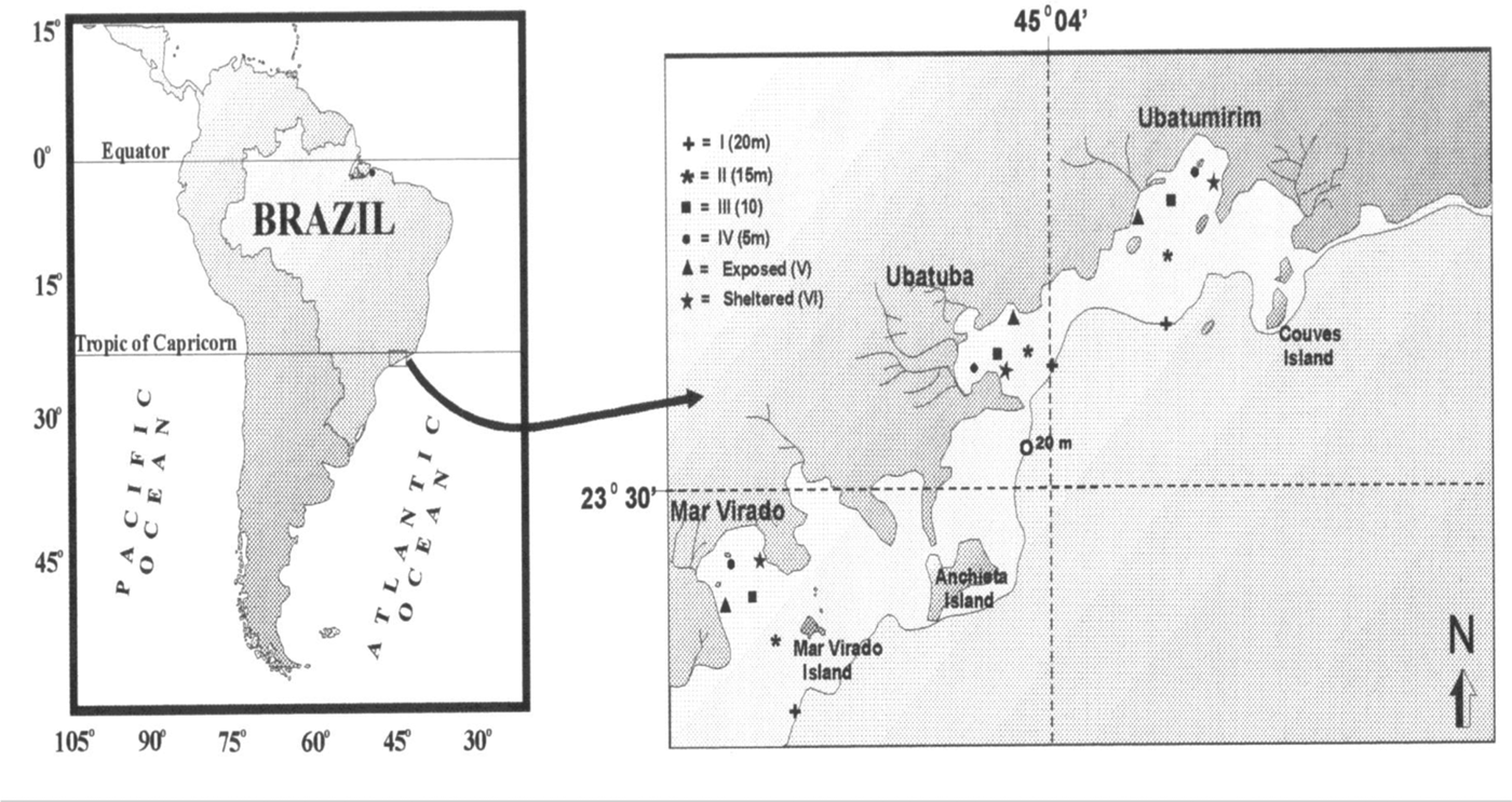
Shrimps were collected monthly from January 1998 to December 1999 from three bays, Ubatumirim (UBM), Ubatuba (UBA) and Mar Virado (MV), all located in the Ubatuba region, State of São Paulo. Each bay was divided into six stations (I, II, III, IV, V and VI), which were selected in order to include the full range of environmental conditions, that is, their position relative to the bay mouth, depth and sediment type; the presence of a rocky wall or beach along the bay shore; the inflow of fresh water; and the proximity of offshore water, that is, open areas with higher salinity. Four of the stations were located at mean depths of 5 m (IV), 10 m (III), 15 m (II) and 20 m (I), and two were established adjacent to rocky shores (an exposed and a sheltered shore, Stations V (9 m) and VI (6.5 m), respectively) (Figure 1). A shrimp-fishing boat equipped with double-rig nets (mesh size 20 mm and 15 mm in the cod end) was used for trawling. At each station we trawled over a 30 min period, covering 18,000 m2.
Map of the Ubatuba region with the indication of stations in each bay.

Environmental factors
Salinity and temperature (bottom and surface water), depth, organic matter content (%) and grain size of sediments were measured at each collection station. The bottom water was sampled using a Nansen bottle. Salinity was measured with an optic refractometer (Atago S/1000) and temperature was recorded (°C) using a mercury thermometer with an accuracy to within 0.1°C. An ecobathymeter coupled with a global positioning system (GPS) was used to record depth (m) at the sampling sites. The rainfall data were sourced from www.ciiagro.org.br. Sediment samples were collected at each station with a Van Veen grab (0.06 m2). Sediment was oven-dried in the laboratory at 70°C for 72 h. In order to analyse grain size composition, two 50 g sub-samples were treated with 250 ml of a 0.2 N sodium hydroxide (NaOH) solution, stirred for 5 min to separate the silt and clay particles, and then rinsed using a 0.063 mm sieve.
Sediment samples were sieved to separate them into: 2 mm (gravel); 1.01–2.0 mm (very coarse sand); 0.51–1.0 mm (coarse sand); 0.26–0.50 mm (medium sand); 0.126–0.25 mm (fine sand); and 0.063–0.125 mm (very fine sand); smaller particles were classified as silt–clay. Grain size categories followed the American standard (Wentworth, Reference Wenthworth1922), and fractions were expressed on the φ scale, thus accounting for the central tendency of sediment samples, e.g. −1 = φ < 0 (gravel); 0 = φ < 1 (coarse sand); 1 = φi < 2 (intermediate sand); 2 = φ < 3 (fine sand); 3 = φ < 4 (very fine sand); and φ ≥ 4 (silt + clay) (Tucker, Reference Tucker1988). Cumulative particle-size curves were plotted on a computer using the φ scale, with values corresponding to the 16th, 50th and 84th percentiles used to determine the mean diameter of the sediment with the formula
 $${\rm Md} = ({\phi _{16}} + {\phi _{50}} + {\phi _{84}})/3$$
Finally, φ was calculated using the formula φ = −log2d, where d = grain diameter (mm) (Tucker, Reference Tucker1988).
The organic matter content (%) was obtained by ash-weighing: three aliquots of 10 g each per station were placed in porcelain crucibles and burned for 3 h at 500°C, and the samples were then weighed again (Mantelatto & Fransozo, Reference Mantelatto and Fransozo1999).
Data analysis
Shrimp abundance (dependent variable) was compared temporally between years and seasons (independent variables): summer (January–March), autumn (April–June), winter (July–September) and spring (October–December); it was also compared spatially between the bays and station collections (independent variables) using an analysis of variance (nested ANOVA) (α = 5%) model, with station nested within region and seasons nested within years. A post-hoc Tukey test was used to assess differences between seasons, bays and stations.
To assess the amount of variation in faunal densities related to a set of habitat environmental characteristics, a redundancy analysis (RDA) was used (Ter Braak, 1996). Previous analysis of the main species showed a linear response in their abundance in relation to the environmental variables used, and so the use of the RDA offers a greater percentage of the variance explained regarding the canonical correspondence analysis (CCA), which is more suitable when there is a unimodal response. The set of environmental variables used in RDA calculations comprised bottom salinity and bottom temperature, organic matter content (%) and grain size of sediments (φ) and rainfall. Only for RDA population was divided into juveniles and adults. However, for spatio-temporal analysis, population was analysed all together.
Tests for homoscedasticity (Levene tests) and normality (Shapiro–Wilk tests) were first performed as pre-requisites for the statistical test. Data were log-transformed prior to analysis (Zar, Reference Zar1999). All the data sets were normally distributed, with homogeneous variances.
RESULTS
Environmental factors
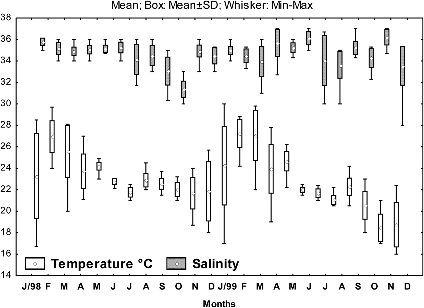
In general, the highest average bottom salinities (>35) were found during the first six months in 1998, except for March, whereas in 1999 the highest values were recorded in April, May, June, September and November. On the other hand, the lowest values—around 33—were recorded during September and October of the first year, and during August and December of the second year (Figure 2). Average salinity values changed according to depth in all three bays, being lowest in shallower locations (site IV = 33.92 ± 1.63 and site VI = 33.56 ± 1.67) and highest in deeper locations (site I = 34.89 ± 1.39 and site II = 34.56 ± 1.33).
Boxplot showing mean, maximum and minimum salinity values and temperature for each month during 1998 and 1999.
Bottom water temperatures were lower in the first year during all seasons except summer. The highest average temperatures were recorded during the summer in both years (26.05 ± 2.23°C in 1998 and 27.33 ± 1.91°C in 1999), and the lowest average temperatures were observed during the spring (21.86 ± 1.21°C in 1998 and 19.37 ± 1.33°C in 1999) (Figure 2). Average temperature values were more homogeneous during the winter, varying between 21 and 22°C (Figure 2).
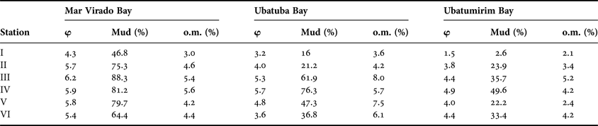
Differences in organic matter content were detected among the bays. The deepest stations (I and II) of the three bays and Station V in Ubatumirim had the lowest levels. However, the highest average percentages of organic matter were obtained at Stations III, IV and VI for the three bays and Station V for Ubatuba and Mar Virado (Table 1).
Mean values of sediment parameters (w, diameter; % silt + clay, mud contents; o.m., organic matter content) for each station in each sampled Bay, from 1998 to 1999.
A trend of a decrease in the amount of mud in the granulometric composition of the sediment was detected in a south–north direction in the sampled bays, that is, northern bays in Mar Virado had a higher fraction of silt and clay (φ > 4) at all sampled points. On the other hand, a predominance of fine and very fine sand associated with silt and clay was observed at most points of UBA and UBM (Table 1).
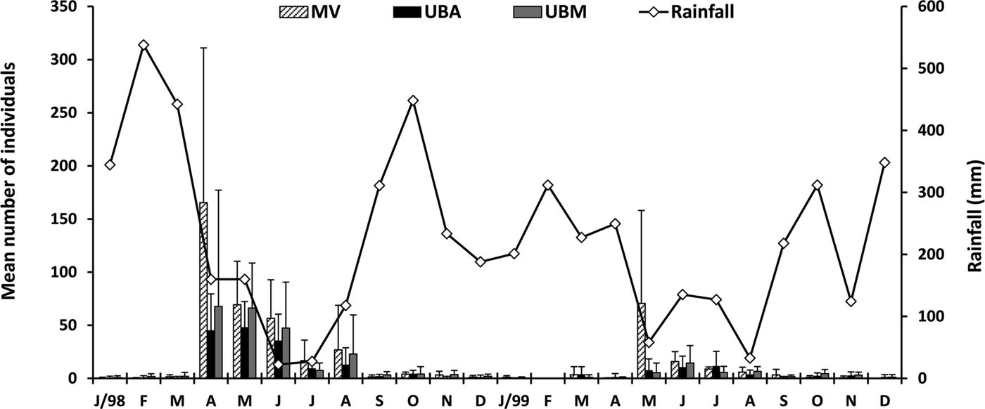
Rainfall was highest during the first year, with a yearly average of 249.44 ± 168.20 mm and with January, February, March, September and October experiencing rainfall of above 250 mm. The second year had an average rainfall of 195.49 ± 101.64 mm and precipitation above 250 mm during the months of February, October and December (Figure 3).
Accumulated monthly rainfall (mm) in the study period, and the mean number of collected individuals each month between 1998 and 1999 in each of the three bays.
Abundance and distribution
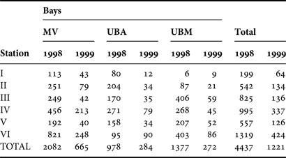
A total of 5658 individuals of L. schmitti were collected during the study period, 4437 in the first year and 1221 in the second year. Approximately 95% of all shrimp were captured in shallow waters, that is, at depths less than 15 m. There were differences in abundance, both temporally with seasons nested in years (nested ANOVA, P < 0.01) (Table 2) and spatially with station nested in region (nested ANOVA, P < 0.01), but there was no statistical difference between the bays (nested ANOVA, P = 0.26) (Table 3).
Results of nested ANOVA for individual abundance (log + 2 transformed) of Litopenaeus schmitti collected in the region of Ubatuba in three bays (MV, UB, UBM), from January, 1998 to December, 1999. Season (year) = seasons nested in years.

d.f., degrees of freedom; MS, mean square; F, MS factor/MS residual; P, probability of significance; α = 0.05.
Results of nested ANOVA for individual abundance (log + 2 transformed) of Litopenaeus schmitti collected in the region of Ubatuba in three bays (MV, UB, UBM), from January, 1998 to December, 1999. Station (bays) = station nested in region.

d.f., degrees of freedom; MS, mean square; F, MS factor/MS residual; P level, probability of significance; α = 0.05.
Litopenaeus schmitti was more abundant in Mar Virado (2747), followed by Ubatumirim (1649) and the bay of Ubatuba (1262) (Table 4). There were more captures at Stations VI and IV of the Mar Virado inlet, at site IV of the Ubatuba inlet, and sites VI and III in the Ubatumirim inlet (Tukey, P < 0.01) (Table 1).
Number of individuals for each station in each sampled bay, from 1998 to 1999.
MV, Mar Virado; UBA, Ubatuba; UBM, Ubatumirim.
The highest abundance was recorded during the autumn and winter of 1998 (95.33%) and 1999 (86.32%) (Figure 3). Except for the winter of the second year, shrimp abundance during these periods differed statistically from other seasons (Tukey test, P < 0.01). In contrast, the lowest abundance was recorded during the summer and spring, particularly in 1999.
Abundance–environmental relationship
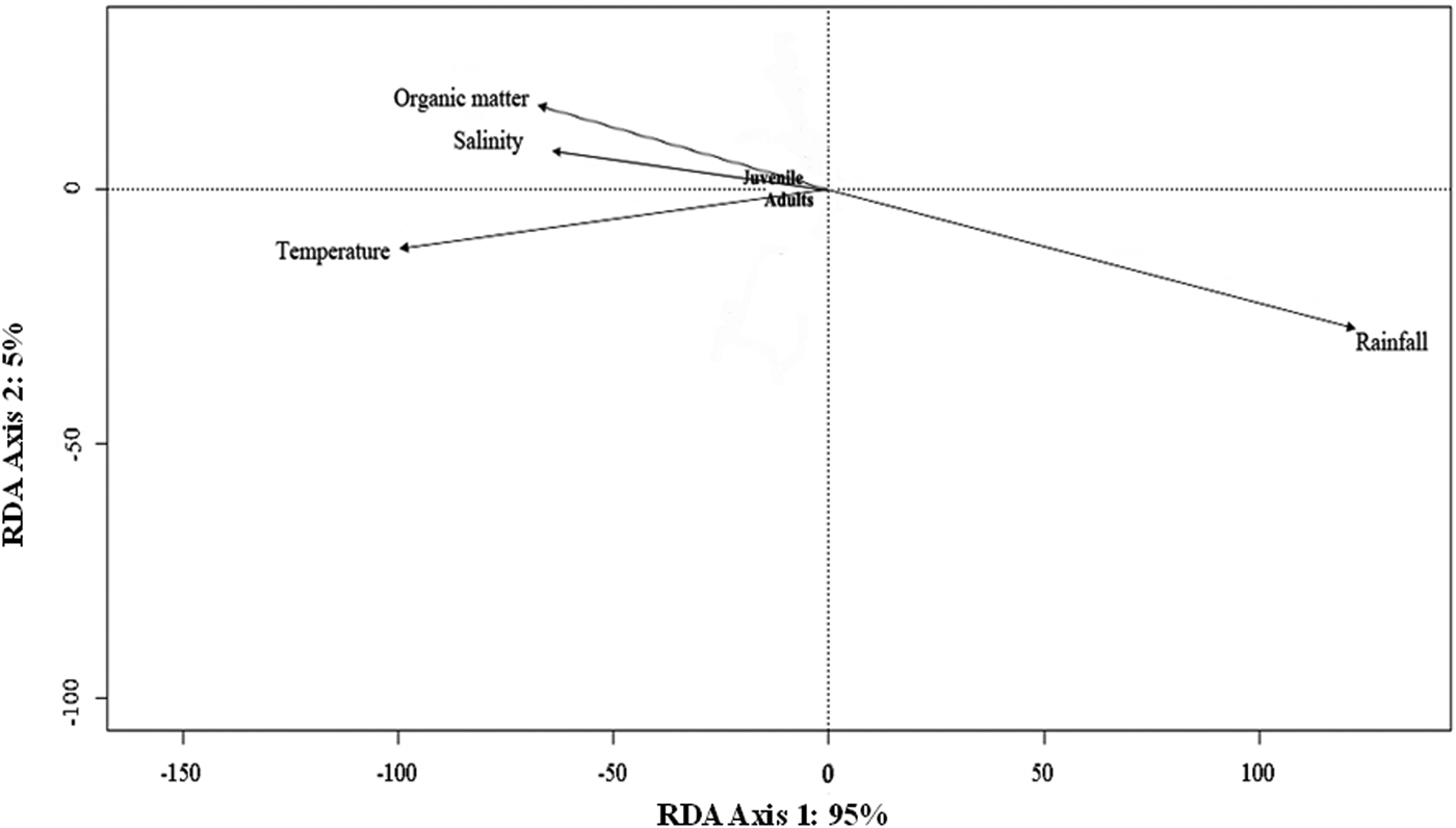
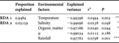
Relation between shrimp abundance and environmental factors shown by redundancy analysis (RDA) is represented by first and second axes in Figure 4. The first axis of biplot graphic explains 95% of total variance of the data, while the second axis explains 5%. The Monte-Carlo test indicated that four canonical axes together (P < 0.005) were significant. These variables are rainfall, temperature, salinity and organic matter (Table 5; Figure 4).
Redundancy analysis (RDA) biplots illustrating the relationship between significant environmental variables and Litopenaeus schmitti collected in the region of Ubatuba in three bays (MV, UB, UBM), from January, 1998 to December, 1999.
Results of redundancy analysis (RDA) of the abundance of Litopenaeus schmitti in relation to environmental variables that explained the most variance of the data collected in the region of Ubatuba in three bays (MV, UB, UBM), from January, 1998 to December, 1999.
Significance codes: (P < 0.05); ***0.001; **0.01; *0.05; . 0.1, 1.
Shrimp abundance correlated positively with organic matter content, salinity and temperature (P = 0.44, P = 0.048 and P = 0.00, respectively), with the highest number of individuals collected from sites with intermediate levels of organic content (4 and 6%) and increasing when the sediment had a higher proportion of fine and very fine sand + clay. Individuals were found at all temperatures, being most abundant in the broad category from 20 to 26°C. In terms of salinity, the highest abundances (4671 individuals) were found in the months with salinity above 35. Abundance was also associated negative with rainfall, given that the analysed population showed a seasonal pattern, with an increase in capture rate in those months following the rainy season (P = 1.56E-23). The summer and spring of both years were characterized by the highest rainfall and the lowest number of captured shrimp (Figure 3).
DISCUSSION
The results of the present study demonstrate stronger affinities between the distribution of the species and rainfall, organic content, temperature and salinity. These results corroborate with many studies on Penaeoidea, such as those of Costa et al. (Reference Costa, Fransozo, Castilho and Fúlvio2005a, b, Reference Costa, Fransozo, Freire and Castilho2007), Castro et al. (Reference Castro, Costa, Fransozo and Mantelatto2005) and Santos et al. (Reference Santos, Severino-Rodrigues and Vaz-Dos-Santos2008), where it was verified that abiotic factors such as temperature and salinity are important in penaeid shrimp distribution. It is possible that the limited variation in the measured average values, particularly in the case of the salinity of the sampled bays, might be due to the small size of the estuaries in the region compared to those of Santos/São Vicente and Cananéia on the southern coast of São Paulo, and to Lagoa dos Patos on the coast of Rio Grande do Sul State (Costa et al., Reference Costa, Lopes, Castilho, Fransozo and Simões2008).
The species shows a stronger preference for sites with a predominance of muddy substrates and intermediate levels of organic matter content. According to Dall et al. (Reference Dall, Hill, Rothlisberg and Staples D1990), water depth, granulometric distribution and the organic matter content of the sediment are frequently interrelated. Fine sediments are found in areas protected from the action of the waves, and have elevated organic carbon content because a large proportion of the silt is composed of organic matter. This organic content can influence the distribution of penaeids, given that it serves as a food source for shrimps (Hindley, Reference Hindley1975).
Most penaeids show this relationship with organic content, such as: Penaeus esculentus Waswell, 1879, Metapenaeus endeavouri (Schmitt, 1926), Melicertus longistylus (Kubo, 1943), Melicertus latisulcatus (Kishinouye, 1896), studied by Gribble et al. (Reference Gribble, Wassenberg and Burridge2007); A. longinaris and X. kroyeri, reported by Costa et al. (Reference Costa, Fransozo, Castilho and Fúlvio2005a, Reference Costa, Fransozo, Freire and Castilho2007); and S. dorsalis, studied by Castilho et al. (Reference Castilho, Furlan, Costa and Fransozo2008b). Fine sediment can facilitate burying activity by individuals of L. schmitti. When buried, these shrimps are protected against predators and spend less energy (Ameeri & Cruz, Reference Ameeri and Cruz1998; Simões et al., Reference Simões, Costa, Fransozo and Castilho2010).
Grains with a larger diameter size are more difficult to move, so that the shrimp spend a greater amount of time and energy in burying activity in this kind of substrate. Species that prefer sediments with the finer texture associated with silt + clay display a mechanism enabling the flow of the exhaling water to revert, removing obstructions from the branchiae before they become impregnated with smaller particles (Ruello, Reference Ruello1973). Costa et al. (Reference Costa, Fransozo, Castilho and Fúlvio2005a, Reference Costa, Fransozo, Freire and Castilho2007), while studying A. longinaris and X. kroyeri, also conclude that grain particle size might be more important to shrimp distribution than the amount of available organic matter in the substrate. This fact was also observed in the present study, given the higher abundance of L. schmitti found in MV, where the sediment is mainly composed of silt and clay at all sampled sites.
In general, the highest shrimp abundances were recorded during the autumn months in both years. This fact can be attributed to the life cycle of the studied species. According to Dall et al. (Reference Dall, Hill, Rothlisberg and Staples D1990), post-larvae enter estuaries and remain in this environment until reaching the juvenile or sub-adult phase and later return to oceanic areas. Capparelli et al. (Reference Capparelli, Kasten, Castilho and Costa2011) confirm this life cycle for the studied region, recording the occurrence of a peak of juveniles at the end of the spring and beginning of the summer in an estuarine river adjacent to the bay of Ubatuba and, three to four months after this peak (autumn and winter), noting a large emigration toward the bay, as well as the observation of seasonal recruitment.
Similar results were obtained for the Cananéia region, where the highest abundances were recorded between March and July (Chagas-Soares et al., Reference Chagas-Soares, Pereira and Santos1995). The same observation was made by Santos et al. (Reference Santos, Severino-Rodrigues and Vaz-Dos-Santos2008), whose results indicate higher abundances between April and June in the region of Santos, São Paulo State.
The results of the present study indicate that, in addition to the influence of life cycle on the temporal distribution of the species, rainfall might also play an important role in determining the onset of their establishment in bay areas. The excessive rainfall during January, February and March of 1998 might have been responsible for the earlier shift of these organisms from the estuary to the bay than in the following year. In 1999, a lower overall rainfall occurred, mainly from February to April, whereas the highest shrimp abundance was recorded from May to July. Santos et al. (Reference Santos, Severino-Rodrigues and Vaz-Dos-Santos2008) obtained similar results, with a higher capture of specimens in months subsequent to the rainy season.
It is possible that elevated rainfall causes a broader salinity gradient, leading to a transition between the lower salinity in the estuaries to the conditions of the bay. Santos & Freitas (Reference Santos and Freitas2004) also observe that the season with the largest abundance of white shrimp in the Lagoa do Papari, in Rio Grande do Norte State, follows the rainy season. The natural pressure of that period in the life cycle, together with the search for increasingly higher salinities, could explain the association between movement (recruitment), concentration of individuals, rainfall and higher fishery yield.
The higher rainfall in 1998 was probably due to the El Niño–Southern Oscillation (ENSO) (Glantz, Reference Glantz2001; Berlato et al., Reference Berlato, Martins, Cordeiro and Oderich2007; Filgueira et al., Reference Filgueira, Neto and Barbosa2007; Britto et al., Reference Britto, Barletta and Mendonça2008). This phenomenon is currently considered to be the main source of short-term climatic variability in the world, occurring on seasonal and inter-annual timescales and leading to droughts and floods around the world. In Brazil, the ENSO is mostly characterized as being associated with intense rains in southern and south-eastern Brazil, and with droughts in the north and north-east (Silva, Reference Silva2001).
A study by Garcia et al. (Reference Garcia, Vieira, Winemiller and Grimm2004) in the Lagoa dos Patos shows that, with increasing rainfall, there is a corresponding several-fold increase in the volume of freshwater discharge into the lagoon, affecting primary productivity in the coastal region of southern Brazil and the fish assemblage in the Lagoa dos Patos. The same could be the case in the bays of Ubatuba, that is, the increase in rainfall might have led to an increase in the influx of freshwater and a corresponding decrease in salinity. This could be reflected in the higher abundance of shrimp collected in this bay in April of 1998 and May of 1999, both of which were months following the rainy season.
Overfishing is another factor which should be taken into account in analysing the inter-annual difference in abundance. In 1998, the highest abundance was recorded in April, when fishing was prohibited. In the following year, individuals were collected in higher abundance in May, with a sharp decline in the month following the fishing season, a period in which the fishing fleet was more active in Ubatuba.
Therefore, it is likely that the El Niño phenomenon led L. schmitti to leave the estuary earlier in April of 1998, increasing its density in the bay; in contrast, in the following year a higher density of the species was detected in May, decreasing markedly in the remaining months due to the opening of the fishing season. Coelho & Santos (Reference Coelho and Santos1994, Reference Coelho and Santos1995), in a study on the life cycle of the white shrimp in Pernambuco State, conclude that individuals born during the summer appear in the commercial fisheries at the end of the autumn or winter of the following year. That observation corroborates the results of the present study.
Our data suggest that, in the region of Ubatuba, the factors that most influence the spatial distribution of the white shrimp are the temperature, salinity and organic matter content conditions of the sediment. Over time, the distribution of individuals seems to be more associated with life cycle and rainfall, given that abundance increases seasonally (autumn–winter) and is stronger in years with an elevated rainfall. In addition, the sampled areas are of fundamental importance to the continuation of the life cycle of this important fishery resource.
ACKNOWLEDGEMENTS
We thank Dr Marcio R. Pie and Proof-Reading-Services.org for great help with the English language. We are also thankful to the NEBECC co-workers for their help during fieldwork All sampling in this study was conducted in compliance with applicable state and federal laws.
FINANCIAL SUPPORT
We are grateful to the Fundação de Amparo à Pesquisa do Estado de São Paulo (FAPESP) for providing financial support (No. 94/4878-8; No. 97/12108-6 No. 97/12106-3 No. 97/12107-0; No. 09/54672-4 and No. 10/50188-8) and to CNPq (Research Scholarships PQ 140335/2012-9 to G.L.B. and PQ2 304784/2011-7 to R.C.C.).