

1. Introduction
The financial crisis of 2008 has created a precarious situation for numerous governments. This is especially true for many municipal governments within the United States, recently highlighted by several high-profile financial problems. Jefferson County, Alabama has become one of the most well-known examples. Unable to raise the revenue necessary to cover its outstanding debt obligations of $4.2 billion, the county filed for bankruptcy on 9th November 2011; becoming the largest of its kind in US history. This event followed, among others, another major municipal bankruptcy when on 12th October 2011 the city of Harrisburg, Pennsylvania (the state capital) was forced into bankruptcy with some $300 million in obligations (The Economist Magazine 3 December 2011, pp. 89). Stockton, California has become the most recent example when in April of 2013 it was allowed to enter into Chapter 9 bankruptcy, thus becoming the largest city by population to ever do so.
These examples only highlight a more recent trend in municipal finance and governance that has resulted largely from the financial crisis. However, this is neither the first time in US history when such local and municipal difficulties have arisen, nor is it the most severe. In fact, the first episode of large-scale municipal default in the United States can be traced back to the Reconstruction era and the panic of 1873, during which time due to a railroad construction and real estate boom, local municipalities drastically increased their overall indebtedness in order to help finance many of these projects and other public works.
However, due to the depression that ensued after the panic of 1873 and the over-borrowing carried on by municipal governments leading up to it, numerous local governments across the country were forced into default, amounting at its peak to nearly 20% of all municipal obligations entering such a state. The aftermath of this debacle was a concerted effort by state governments to find solutions so as to ensure that such an outcome would not be repeated. The response was a multitude of constitutional amendments that either prohibited or greatly constrained municipal governments from issuing debt on a similar scale as they had prior to the panic and ensuing depression.
Given these outcomes, the scope of this study is to understand the impact that these newly adopted constitutional constraints had on municipal borrowing costs after their adoption, and also to understand how market participants actually perceived these constraints (whether or not they were considered binding). In order to do so, this current paper empirically analyzes the impact these constitutional constraints had on municipal borrowing costs observed with unique data taken from a number of financial markets throughout the United States between 1880 and 1890.
Overall, the study finds that, in general, explicit creditor guarantees, constitutionally imposed hard budget constraints, and strict debt limits appeared to have most consistently reduced overall borrowing costs. It would also appear that constraints, which limited the ability of municipal governments to raise revenue through taxation, actually increased borrowing costs. Most interesting is the impact that these constraints had on defaulting relative to non-defaulting cities, which suggests that stringent borrowing and lending constraints as well as creditor guarantees appear to have led to much lower borrowing costs.
This adds to several important existing strands of literature. The first is that of fiscal federalism, begun with the seminal work of Tiebout (Reference Tiebout1956), and culminating with the literature on market preserving and fiscal federalism (Oates, Reference Oates1972, Reference Oates2005; Qian and Roland, Reference Qian and Roland1998; Weingast, Reference Weingast1995). This literature suggests that through interjurisdictional competition, present especially under a system of federalism, policies that are detrimental to economic growth and development will be checked, as suboptimal policy decisions in one jurisdiction have the unintended consequence of leaving citizens in a neighboring jurisdiction relatively better off. In this context, suboptimal policies pursued by a subsection of municipalities leading up to the panic of 1873 left many of them relatively worse off compared to municipalities which pursued more time-consistent public policy. This in turn left the respective state economically weakened on a comparative basis, which created the incentive for those same states to impose binding constitutional rules on their respective municipal governments.
This motivates the second strand of literature which this paper expands on. Specifically, it is the importance between hard and soft budget constraints on lower level governments and jurisdictions, which is especially important within a system of federalism (Goodspeed, Reference Goodspeed2002; Kornai et al., Reference Kornai, Maskin and Roland2003; Oates, Reference Oates2005; Poterba, Reference Poterba1994, Reference Poterba1996; Poterba and von Hagen, Reference Poterba and von Hagen1999). Here, it is suggested that in order to minimize the impact of fiscal shocks on an economy, the central authority must commit to a hard budget constraint, and not bailout lower level governments when they do face fiscal difficulties. In so doing, the central government creates an incentive of fiscal discipline and is better able to avoid moral hazard problems associated with softer budget constraints.
Another body of literature that this paper adds to is the branch of public finance which seeks to understand the impact that fiscal institutions have on budgetary outcomes. Much of this literature attempts to analyze how fiscal restrictions impact the level of debt within a state, most of them finding that states with stricter anti-deficit and anti-spending measures have lower overall debt burdens and reduced deficits (Alesina and Bayoumi, Reference Alesina and Bayoumi1996; Bohn and Inman, Reference Bohn and Inman1996; Eichengreen, Reference Eichengreen1992; Eichengreen and Bayoumi, Reference Eichengreen and Bayoumi1994; Kiewiet and Szakaly, Reference Kiewiet and Szakaly1996). Still others examine the relationship between fiscal institutions and financial markets (Bayoumi et al., Reference Bayoumi, Goldstein and Woglom1995; Eichengreen, Reference Eichengreen1992; Goldstein and Woglom, Reference Goldstein, Woglom, Canzoneri, Grilli and Masson1992; Johnson and Kriz, Reference Johnson and Kriz2005; Lowry and Alt, Reference Lowry and Alt2001; Poterba and Rueben, Reference Poterba, Rueben, Poterba and von Hagen1999). In general, these works find that debt and expenditure limitations lead to lower borrowing costs for states, while tax limitations increase those same costs. There is also evidence to suggest that debt referenda lead to relatively higher debt levels and higher borrowing costs (Kiewiet and Szakaly, Reference Kiewiet and Szakaly1996).
Finally, a large body of literature examines the relationship between tax and expenditure limits (TELs) and other fiscal limitations on government size and growth of government, government spending patterns, and overall debt structures of both state and municipal governments (Abrams and Dougan, Reference Abrams and Dougan1986; Bails and Tieslau, Reference Bails and Tieslau2000; Cabases et al., Reference Cabases, Pascual and Valles2007; Epple and Spatt, Reference Epple and Spatt1986; Farnham, Reference Farnham1985; Kousser et al., Reference Kousser, McCubbins and Moule2008; Mullins, Reference Mullins2004; Mullins and Joyce, Reference Mullins and Joyce1996; Shadbegian, Reference Shadbegian1996, Reference Shadbegian1998). These studies are in general mixed in their findings that TELs and other similar restrictions are effective in carrying out their intended purposes, especially in constraining government growth and spending.
The remainder of the paper is structured as follows. Section II gives an historical overview of the fiscal policies that municipal governments were engaging in through the mid-19th century. The overview continues with a brief discussion of the panic of 1873 and its impact on municipal finances, the result being large-scale defaults across the United States. Finally, the section provides an analysis of the aftermath of this episode, describing the push for state constitutional change meant to deal specifically with the municipal debt crisis. Section III describes the data employed as well as the empirical estimation models. Section IV presents the results, providing an interpretation and explanation of them. Section V concludes the study.
2. Historical background
The United States in the 19th century was a time filled with large-scale public/private partnerships in the economy. Although the federal government by and large avoided any direct role, much of this a result of extreme sectionalism that existed especially prior to the Civil War, states during the antebellum period invested heavily in their economies.Footnote 1 This investment generally came in the form of aid to infrastructure projects (dubbed internal improvements), and banking. These policies persisted until the panic of 1837 and through the subsequent depression that began in 1839.
It was through the depression of 1839 that many states found themselves financially constrained, generally as a result of failed investments in internal improvement and banking projects. The result of this depression was default on debt obligations by eight states and one territory, of which five of these eventually repudiated all of part of those debts. The aftermath of this episode was a period of constitutional change which placed a number limits and constraints on a state's ability to invest in similar projects, incur debt in the future, and fund projects through ‘taxless finance’ (Goodrich, Reference Goodrich1950; Larson, Reference Larson2001; Wallis, Reference Wallis2005).
However, as these constitutional limitations on state governments persisted, a new form of public assistance slowly began to seep into the economy. This came in the form of lower-level municipal aid, generally in the form of town, city, and county financial assistance (Gillette, Reference Gillette2003; Pinsky, Reference Pinsky1963; Secrist, Reference Secrist1914).Footnote 2 Much of the assistance was geared toward railroad construction, as this new form of transportation was considered by many to be the best means by which to increase local economic activity. It was also believed that such public assistance would net large profits and perpetual revenue streams for those municipalities that made the investments, greatly increase local property values, and with it tax revenue (Burhans, Reference Burhans1889).
Thus, over roughly three decades from 1850 to 1870, the desire to support privately developed internal improvements through public aid was born, with Missouri taking the lead by passing a general act granting municipal aid to railroads in 1853; followed by Arkansas in 1855, Alabama in 1868, Kansas in 1869, and Michigan in 1869 (Hillhouse Reference Hillhouse1936). Still further borrowing was carried on by municipal governments for numerous other purposes including the paving and sewering of streets, and other forms of city construction and development (Goodall, Reference Goodall1964; Raymond, Reference Raymond1932; Studenski, Reference Studenski1930).
The public assistance took a multitude of forms, but was generally done by issuing municipal debt on behalf of private companies or through stock subscriptions. Under this system, municipal bonds would either be traded to private companies for the stock of the company, or the debts of those companies would be guaranteed with municipal credit outright (Pinsky, Reference Pinsky1963). Generally upon receiving municipal bonds, these companies were allowed to dispose of those bonds as seen fit; often times seeing these bonds sold in eastern markets at 65 to 70 cents on the dollar (Pinsky, Reference Pinsky1963).
Under this system, these debts were ultimately the obligations of those railroads, with the public credit used only to help in raising the necessary capital for those companies. Though this system could function if railroads remained solvent and paid off those debts, it would be up to those local governments to cover the obligations in the event that the private company failed. Of course, with railroad default and the loss of municipal revenue that was soon created as a result of the panic of 1873, many municipalities were simply unable to cover their own debt obligations as they came due, resulting in much of the default, which occurred throughout the 1870s.
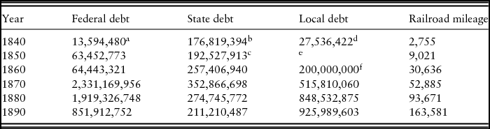
As these policies persisted they became self-reinforcing, as it was believed that by not providing massive public municipal assistance, a municipality was curtailing its economic potential with slower growth and development (Goodall, Reference Goodall1964; Hillhouse, Reference Hillhouse1936; Secrist, Reference Secrist1914). However, as these obligations increased throughout the later half of the 1800s, they created an ever-growing municipal debt burden, which can be seen in Table 1.
Federal, state, and local indebtedness in dollars and total railroad mileage

Data from U.S. Census Bureau 1870, 1880, and 1890.
aData for 1842;bData interpolated from 1839 and 1841 data;cData for 1853;dData for 1843;eNo data available;fEstimated.
Whereas in 1840 municipal indebtedness was estimated to be roughly $27 million, by 1860 this had grown to almost $200 million, over $515 million by 1870, and almost $850 million by 1880. This last figure was nearly three times the total state indebtedness at the time. Although such a situation was able to persist as long as the economy expanded and railroad companies remained solvent, this situation would and soon did change as a result of a severe economic downturn in 1873. The overall result rapidly deteriorated municipal finances.
The panic of 1873 was an acute banking panic, which led to a severe nationwide depression for several years. As the depression persisted, multitudes of railroad failures occurred, land values plummeted, and as a result of previous policy numerous municipalities were left with large debt commitments backing those failed railroads, reduced tax bills as a result of lower property values, and therefore, no ability to remain financially solvent.
For example, while the period 1868–1870 saw only one railroad enter receivership in each of those years, another three entered receivership in 1871, 12 in 1872, and over the first nine months of 1873, 35 had defaulted. By 1874, nearly 25 percent of all railroad bonds were in default (Swain Reference Swain1898). The impact that this had could be seen across the states as municipalities began defaulting on those and other guaranteed debt obligations en masse. Overall, it has been estimated that an amount of somewhere between $100 and $150 million in outstanding debt obligations (roughly 20% of all municipal debt obligations) was in default by the end of the 1870s (Chatters, Reference Chatters1933; Hillhouse, Reference Hillhouse1936).
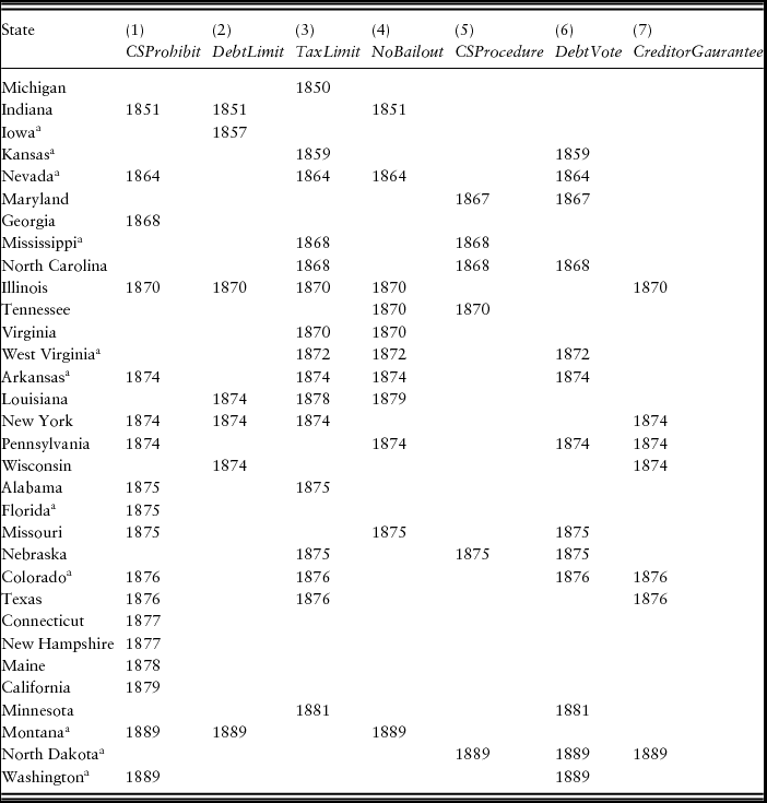
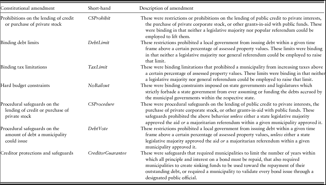
The result of these municipal difficulties and the ensuing defaults that occurred led to significant efforts to constitutionally constrain this behavior, much in the manner that the states had been after the depression of 1839. Table 2 provides a list by state showing when each amendment was adopted and the date when the amendment was adopted. Appendix 1 provides a brief description of each type of constitutional amendment that was passed, as well as a shorthand name to distinguish each of these amendments throughout the paper.Footnote 3
Constitutional constraints by state and year
aDenotes no municipal data available for those state.
As can be seen from Table 2, 13 of the 32 states that constitutionally constrained municipal debt did so within five years after the panic of 1873. Several others did so upon their entrance into the Union.
The first set of amendments this work focuses on is outright prohibitions of either the lending of credit or the subscription of stock ownership with public money into private companies. A total of 17 states strictly prohibited municipalities from issuing debt on behalf of private companies or from subscribing to the stock of such companies. As suggested, it was initially believed that the development of a railroad through a community would lead to increased economic activity, with the returns on investment far outweighing the initial investment itself. This was especially the case as most of the obligations were to be serviced by the railroads, repaying them once they completed construction. However, after the panic of 1873 and the subsequent railroad defaults, it was quickly realized that many of these projects proved to be either unprofitable or unobtainable. Unfortunately, these debts were still obligations of those municipalities, the only method left after the investments failed by which to pay the accruing interest and principal was through heavy taxation (Secrist, Reference Secrist1914).
Multiple states also imposed strict tax limits on the amount a municipality could raise based on a certain percentage of assessed property values. Prior to the panic of 1873, many municipalities maintained lower rates of taxation, even in the face of mounting debt obligations. However, rather than increase the rate of taxation on citizens, these municipalities would generally refund their debts as they came due by issuing more debt. Unfortunately, with the panic and following depression municipalities were forced to drastically increase tax rates on reduced property values. This along with the general mood of the time regarding municipal indebtedness in general played a role in the adoption of these restrictions.
For instance, in his annual message to the legislature, then Governor Hayes of Ohio noted that between 1872 and 1876 municipal taxation had increased over 37% and indebtedness almost 190%. As a result, he pressed upon the legislature the need to push forward constitutional amendments meant to limit both. Specifically he called for ‘A judicious limitation of the rate of taxation which local authorities may levy . . . [to] be strictly adhered to and allow no further indebtedness to be contracted’ The New York Times (NYT (11 January 1876).
A number of states also explicitly imposed hard budget constraints on municipal governments within their constitutions. Although no state through the period had assumed the debts of its municipalities, there were numerous attempts to push state governments to do so. For example, the New York Times (1 February 1878) reported that a bill had been presented before the state legislature of New York, which would have had the state government assume some $27 million in municipal debt. In response to much of this push for assumption of local debt, many states included hard budget constraint clauses into their constitutions meant to combat the problem.Footnote 4
The final set of restrictions were limitations on the maturity of bond issues, the creation of sinking funds, and requirements that municipal bonds be registered with a state or county official in order to guarantee their validity. These first two constraints, at least presumably, were put in place in order to shift a larger portion of the debt burden back to current taxpayers. For example, although initially municipalities had issued bonds maturing anywhere from 10 to 20 years, as the push for public assistance began to peak these maturity dates were shifted further and further out, with some reaching well over 100 years (Studenski, Reference Studenski1930).
Although it is difficult to ascertain the actual size of the sinking funds, by 1881 the sinking fund within New York City had grown to over $35 million (The Bankers’ Magazine and Statistical Register (BMSR) May 1884). Furthermore, in regard to this and other sinking funds, the BMSR noted that
‘Where it [a sinking fund] exists it is certain that money will be accumulated for the discharge of the indebtedness there existing; whereas if such a system did not exist, nothing perhaps would be accumulated. In other words, the sinking fund system when once adopted, if properly executed, requires the city or government adopting it to raise money for the discharge of its obligations. Of course whatever money is paid out must be paid out by the taxpayer.’ (BMSR, May 1884).
Another amendment which many states passed required that the validity of a bond issue be proven before the debt or bonds could be issued. Generally, this came in the form of either requiring a state or county officer to certify the validity of the issue. After the rash of municipal defaults swept the country, many bondholders found they had little legal recourse, as many times county and state judges would hold void a series of bonds that had been issued on technical grounds, leaving bondholders with no ability to collect their outstanding debts (and leaving outstanding bonds in a state of de facto repudiation; Adams, Reference Adams1887). For example, a number of counties in Arkansas attempted to fight the collection of $2 million in bonds by arguing that the bond issues were void as the copyist of the legislative enabling act had substituted an immaterial three-letter word for a two-letter word into the authorizing act (Chatters, Reference Chatters1933). This argument was upheld by the state courts.
For many states if they did not outright prohibit specific actions regarding municipal indebtedness, they created strict procedural safeguards before debt could be issued. Most of these safeguards came in the form of a municipal referendum placed on a ballot requiring some type of majority assent before debt could be raised or aid could be issued. These requirements ranged from simple majority requirements of the legislature, a majority vote of qualified voters in the municipality, some supermajority of qualified voters, or some combination of the three. Not only was this a requirement of a bond issue, it was also many times a requirement necessary before any debt could be issued or stock subscribed to on behalf of private corporations or for other internal and municipal improvement projects.
Given all of this, the question then remains: how much and to what extent were they effective in carrying out their stated goals? The next section attempts to more formally answer this question empirically.
3. Data and methodology
Data
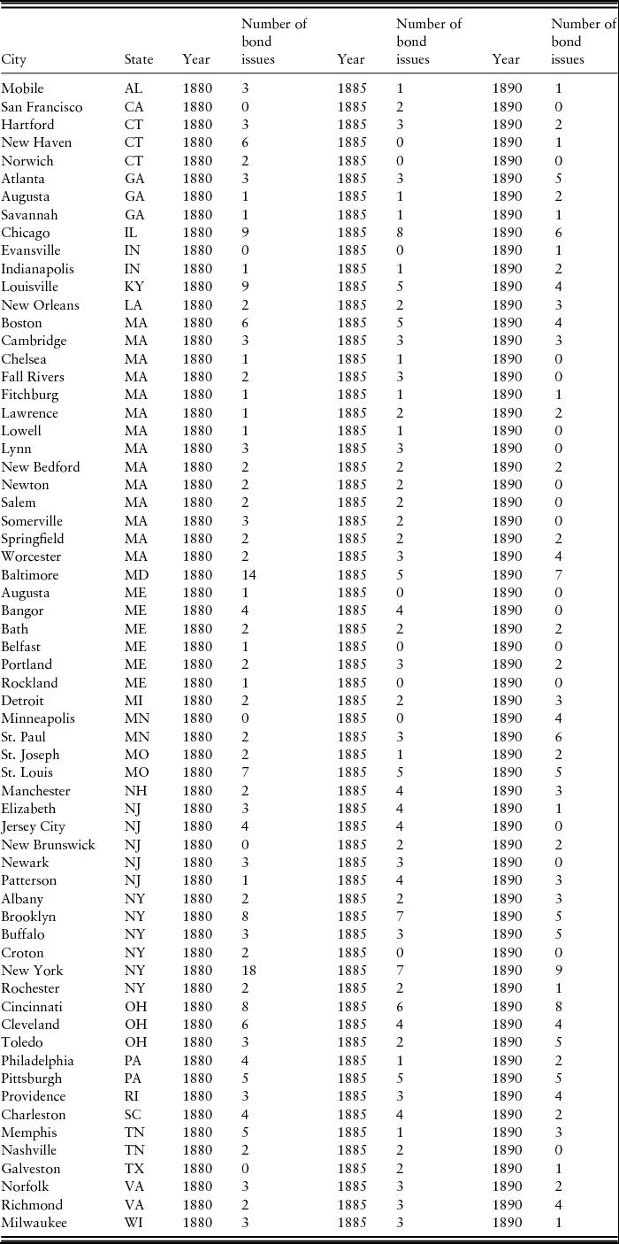
In order to test the impact that the constitutional rules mentioned above had on municipal fiscal outcomes, I have compiled a unique dataset of bond prices for a number of both defaulting and non-defaulting US cities as they traded in the secondary markets in New York and several other cities, for the years 1880, 1885, and 1890.Footnote 5 These data have been hand collected from the Financial and Commercial Review, which was a weekly business and financial periodical published in New York City. This publication listed a large number of municipal bond prices from across the country. I analyze these data with pooled-OLS regressions, in intervals of six months for each year, looking at the months of April and September. This creates a total of 1,001 observations in the sample.Footnote 6
The current study uses as the dependent variable the average yield to maturity (YTM) for each bond listed. This average comes from the fact that each issue may have had multiple closing prices listed during every month under review, given the weekly nature of the publication and listed prices. Thus, I average each observation over the associated month to come to one YTM value for each observation.
Furthermore, these months are used as they are exactly six months apart, and since trading was relatively heavier during spring and fall months, there are a relatively large number of observations and also a sizeable number of observations for cities that traded less frequently. As a caveat, it was not possible to ascertain the interest rate for 14 observations employed. Therefore, to overcome this problem, the coupon rates for the remaining observations available for that city were averaged. This average coupon rate is then assumed to be the coupon rate of the missing observation.
Also, there were a number of issues for which no maturity date was listed. In order to overcome this problem, each missing issue is assumed to have a maturity date of 30 years from the first date in which a bond was listed. For example, if a bond is listed in the Financial Chronicle in 1880, it is given a 30-year maturity date, and then with the 1885 data it is assumed to mature 25 years from that date.Footnote 7
Along with the constitutional provisions, to be discussed in greater detail below, I also include a set of 12 control variables meant to capture socioeconomic differences between cities in the sample, and also financial factors which would impact a municipalities’ borrowing costs. The first control variable is a dummy variable for whether or not a city in the sample defaulted. This would have a profound impact on a city's bond yield, in general causing it to rise significantly. The information on these defaults was taken from several sources including the Commercial and Financial Chronicle, Hillhouse (Reference Hillhouse1930, Reference Hillhouse1936), and Dean (Reference Dean1912). The second variable is a regional dummy for whether a city was located within a former state of the Confederate States of America. Given that these states lost the American Civil War, the result being in many instances a devastated economy and difficulty in raising revenue, then ceteris paribus these southern cities would also have higher bond yields.
A third control is the year in which a municipality was incorporated as a city. This variable is meant to help proxy for the extent of economic development within a given municipality, as the older a city is, the more economically developed and integrated it would be with the rest of the country.
Two additional socioeconomic control variables included are per capita debt and per capita assessed property valuations. These variables were compiled from the Commercial and Financial Chronicle, taken from its bimonthly and later quarterly investor's supplemental magazine. This magazine gave a detailed breakdown of each municipal government that it provided bond data for. The first is included because as per capita debt increases, it should increase a bond's yield. Per capita assessed property values are included as higher property values would lead to increased potential revenue for a city in the form of larger tax returns. Given this, it may be relatively easier for a city to meet its outstanding debt obligations.Footnote 8
Several other control variables are also included in the analysis. The first is the municipal tax rate imposed by each municipality, while the second is whether or not a municipality was located within a home rule state. During the later half of the 19th century, a major debate had arisen regarding state and municipal relations and the scope of municipal government in general. Thus, over this period several states either constitutionally or statutorily passed home rule laws, which greatly enhanced municipal autonomy and also the ability to incorporate.
Finally, I also include control variables for whether or not a bond was issued before the panic of 1873, whether or not a constitutional constraint was adopted before the panic of 1873, whether or not a bond under observation was maturing within the given year under analysis, and whether the observation was from the month of April. Each of these is represented with a ‘1’ if yes, and ‘0’ otherwise.
The first main variable of interest considered is whether or not a state prohibited the lending of credit or stock subscriptions by a municipality, represented by CSProhibit. The second variable represents whether or not a state strictly prohibited municipal debt above a certain percentage of the assessed property value, represented by DebtLimit. The third prohibition is whether or not a state imposed a strict limit on the tax rate that a municipality could impose on the assessed value of property, represented by TaxLimit. The fourth restriction is whether or not a state imposed a hard budget constraint on municipalities, represented by NoBailout. In order to quantify these four variables, each takes a value of ‘1’ if a state had imposed such a constraint and a ‘0’ otherwise.
The final three main explanatory variables of interest represent a set of constitutional safeguards that states placed on municipal governments. As noted, many times states opted, instead of prohibiting certain behavior outright, to rather require more procedural steps before municipal debt could be issued. Thus, the first procedural safeguard employed, represented by CSProcedure, is whether or not the state had some type of majoritarian voting requirement that had to be met before a municipality could lend credit or subscribe to the stock of private companies. Here, the variable is represented with a ‘1’ if a state required either a majoritarian referendum or legislative majority, and a ‘0’ otherwise.
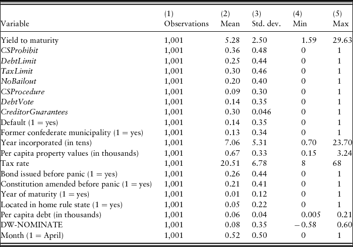
The sixth variable, CreditorGuarantee, represents whether or not a state required some procedural safeguard for the repayment of debt, or creditor protection clause. With this, is included whether or not a state required a municipality to create a sinking fund before it could issue debt, whether or not a constitution required a strict limit on the time to maturity of a debt, and finally whether a municipality had to prove the legality of a bond issue by officially registering it with either a state or county official. Again, if a state required any one of these three safeguards, it is coded with a ‘1’ and a ‘0’ otherwise. The final variable, represented by DebtVote, specifies whether or not a state constitution imposed a mandatory debt limit based on the assessed value of real property within a municipality, but then allowed this limit to be raised with the assent of a specified voting bloc. Table 3 provides the summary statistics for each of these control variables as well as the dependent variable and main variables of interest.
Summary statistics
Estimation specifications
Given the nature of the variables under consideration, it is important to analyze how much a default within a city or municipality may impact the probability that a state passes any of the constraints discussed. However, this requires aggregating a large amount of municipal information up to the state level, which may prove problematic. In order to deal with this issue, I simply analyze each constitutional variable in the year 1890 in order to avoid any variation in those variables over the sample. Furthermore, I use two separate measures that should capture the extent to which municipal defaults within a state may have influenced the adoption of a given constitutional rule.
These variables were both compiled from Maurice B. Dean's Municipal Bonds Held Void, which was a compilation of all municipal bonds that were held void within a state through the 19th century. The first variable is simply a raw count of the number of municipal bonds held void within a state converted to a per capita basis using the state's population for 1890. The second is the actual dollar amount loss on those voided bonds also converted to a per capita basis. Overall, given that there are seven constitutional constraints being analyzed, this provides 14 separate regressions. The probit model used to examine this issue takes the following form:
 \begin{equation}
\Pr \left( {Y_i = y_i {\rm |}x_i } \right) = \alpha + \beta _1 X_i + \varepsilon _i ,\end{equation}
Next, in order to investigate the impact that each of the constitutional rules had on municipal bond yields, this paper employs the following model:
 \begin{eqnarray}
\textit{Bondyield}_{it} &=& \alpha + \beta _1 \textit{CSProhibit}_{it} + \beta _2 \textit{DebtLimit}_{it} + \beta _3 \textit{TaxLimit}_{it} \nonumber\\
&&+ \beta _4 \textit{NoBailout}_{it} + \beta _5 \textit{CSProcedure}_{it} + \beta _6 \textit{CreditGaurantee}_{it}\\
&&+ \beta _{7} \textit{DebtVote}_{it} + \gamma Z_{it}^{'} + \varepsilon _{it} \nonumber
\end{eqnarray}
t = 1880, 1885, 1890, where Bondyieldit is the average bond's YTM for the months of April and September of each of the corresponding years and Z′it represents the control variables discussed.
Along with these specifications from equation (2), I also break the variables down into two separate packages based on whether they were outright prohibitions of specific behavior or procedural safeguards against the behavior. Therefore, I also look at the first four and final three constitutional constraints from equation (2) within separate regressions.
A final empirical specification employed takes the following form:
 \begin{eqnarray}
Bondyield_{it} &=& \alpha + \beta _1 Amendment_{it} + \beta _2 Default_{it} \nonumber\\
&& + \beta _3 Amendment^*Default_{it} + \gamma Z_{it}^{'} + \varepsilon _{it}\end{eqnarray}
t = 1880, 1885, 1890.
Here, Amendment_{it} represents each of the constitutional amendments specified from equation (2), while Default_{it} represents whether or not a city defaulted. Finally, Amendment*Defaultit is an interaction term between each of the amendments and whether a city defaulted. This variable is meant to capture the relative impact that each of these amendments had on a city that defaulted as compared to a non-defaulting city.
Estimation issues
One issue which arises from this analysis is the potential endogeneity of the constitutional rules themselves, per capita debt, and also per capita assessed property values with the bond yields being studied. Therefore, as a first step to mitigate the potential endogeneity of those fiscal rules, I also include a variable to proxy for voter preferences, which follows from Poterba and Rueben (Reference Poterba, Rueben, Poterba and von Hagen1999). In so doing, it may be possible to reduce any correlation which may exist between both fiscal outcomes and fiscal constraints. This occurs as it may minimize the observed correlation between the fiscal rules and borrowing costs faced by a municipality, to a correlation between those variables and an omitted third variable (that being voter preference for a given fiscal outcome) (Poterba and Rueben, Reference Poterba, Rueben, Poterba and von Hagen1999).
Here, this paper uses the DW-NOMINATE score for the congressmen sent to the U.S. House of Representatives for each municipality under review.Footnote 9 First developed by Poole and Rosenthal (Reference Poole and Rosenthal1985), these scores now run from the 1st to the 111th Congress, and provide a score for the ideological disposition of each congressman based on his or her roll call voting record.
Furthermore, I also employ a number of instrumental variables for each of the endogenous variables and a two-stage least squares regression approach to help mitigate the endogeneity issue. For the constitutional constraints, I have attempted to find a number of instruments that would influence the adoption of each of these constraints, but not the fiscal outcomes that emerge.
The first instrument I employ is whether or not the previous state constitution had a similar constraint against state government action to the one imposed on municipal governments. As noted, a number of states in the early 1840s defaulted on their obligations, which led to numerous constitutional constraints on the issuance of state debt. They were largely similar to the ones that would later be imposed on municipal governments. Therefore, I include a dummy variable for whether or not a state government was faced with a similar constraint.Footnote 10 In this vein, I also include a dummy variable for whether or not a state government defaulted during the economic crisis of the 1840s, which may have an impact on the decision to later adopt municipal constraints as well.
Next I include an instrument for the amendment process within a state. Specifically, it is a dummy variable for whether or not a constitutional amendment would only be adopted after a state legislature voted for the amendment over two legislative sessions. Ultimately, the more difficult it is to amend a constitution, the less likely will it be that a given amendment passes. I also include an instrument for the size of the state legislature. The larger the legislature, the more difficult it may be to pass a given amendment. This information was taken from Burnham (Reference Burnham1984). The final two instruments I include for the fiscal rules follow from Poterba and Rueben (Reference Poterba, Rueben, Poterba and von Hagen1999) and are the year in which a state entered the Union and the year a state constitution was adopted. Both of these should pick up differences between states, which may affect the adoption of a given constitutional rule.
I also include several instruments for per capita debt and property values, which draws directly from Capeci (Reference Capeci1991; Reference Capeci1994), Metcalf (Reference Metcalf1993), and Bayoumi et al. (Reference Bayoumi, Goldstein and Woglom1995), all of whom also studied factors that impact municipal and state bond yields and borrowing costs. These instruments include the lagged variables for both per capita debt and property values as well as the population growth rate of each municipality.Footnote 11
4. Results and interpretation
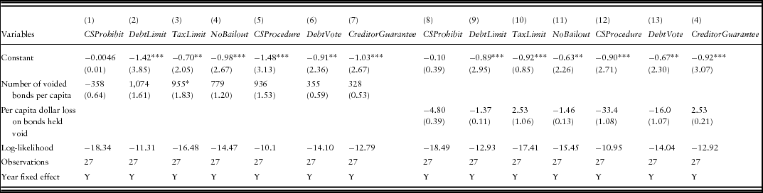
Table 4 first provides the results from equation (1) for the probit analysis.
Probit results
Absolute value of z-statistic in parentheses.
***p < 0.01; **p < 0.05; *p < 0.1.
Here, the results do not generally seem to suggest any statistically significant relationship between a municipality defaulting and a state adopting some constitutional constraint. The only exception is for the TaxLimit variable, which suggests that as the number of voided bonds per capita increases, there may be a greater likelihood that a state adopts such a constraint. However, this result is only weakly significant. Thus, there does not seem to be much reason to believe that there is a significant relationship between default and any of the constitutional rules.
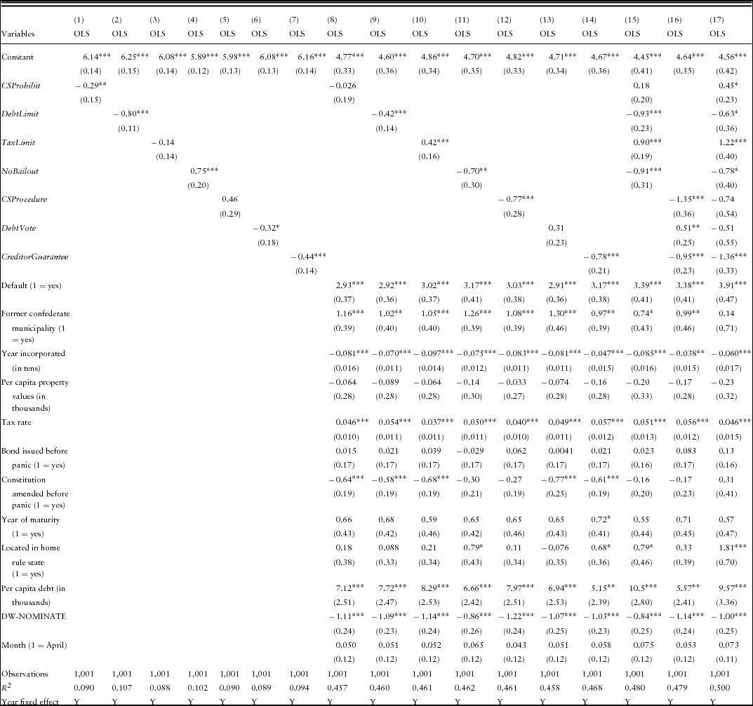
Next, Table 5 provides the OLS results for each of the seven constitutional explanatory variables run against the dependent variable separately and combined, both with and without control variables.
Individual constitutional variables with and without controls; OLS results-dependent variable = average yield to maturity
Robust standard errors in parentheses.
***p < 0.01; **p < 0.05; *p < 0.1.
Columns 1–7 consider each constraint run individually without controls against the dependent variable. Columns 8–14 provide results for each constraint while also including all of the control variables. Finally, column 15 combines four of the constraints (CSProhibit, DebtLimit, TaxLImit, and NoBailout), column 16 combines the remaining three constraints (CSProcedure, DebtVote, and CreditorGuarantee), while column 17 combines all seven constitutional variables
Overall, the results indicate a number of interesting implications. Specifically, DebtLimit and CreditorGuarantee variables consistently resulted in negative and statistically significant results, suggesting that each constraint lowered municipal borrowing costs anywhere from 42 to 93 basis points and 44 to 136 basis points, respectively. Furthermore, both TaxLimit and NoBailout variables also had relatively consistent results. For three of the four specifications, both of these suggested that such a constraint increased borrowing costs between 42 and 122 basis points for TaxLimit and lowered borrowing costs between 70 and 91 basis points for NoBailout.
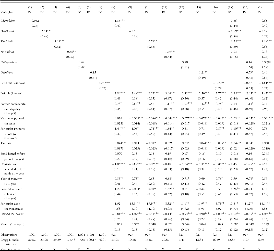
Next, Table 6 provides the second stage instrumental variable regression results for the OLS estimation in Table 5.Footnote 12
Individual constitutional variables with and without controls; IV results-dependent variable = average yield to maturity
Robust standard errors in parentheses.
***p < 0.01; **p < 0.05; *p < 0.1.
The layout of Table 6 follows that of Table 5. Overall, the results are generally consistent with those found in Table 5 for the OLS analysis. The only major differences that do occur are found in columns 1–7 for each of the constitutional variables without controls. Under that specification, the sign coefficients for the variables DebtLimit, TaxLimit, and CreditorGuarantee flip. Outside of those, the only differences on the sign coefficients that do emerge between the tables are in columns 12, 16, and 17 for CSProcedure and column 15 for CSProhibit. Although the statistical significance on several of the variables also changes, this may generally be due to the inflated standard error that resulted from the instrumental variable estimation and the fact that under these specifications the instruments become somewhat weak.
The most consistently significant results seem to be for TaxLimit which is again positive and significant for all results, suggesting such a constraint increases borrowing costs between 71 and 307 basis points. Furthermore, although somewhat weaker than before, the variables DebtLimit, NoBailout, and CreditorGuarantee reduce borrowing costs in three of four specifications each, between 10 and 179 basis points, 18 and 179 basis points, and 47 and 181 basis points, respectively.
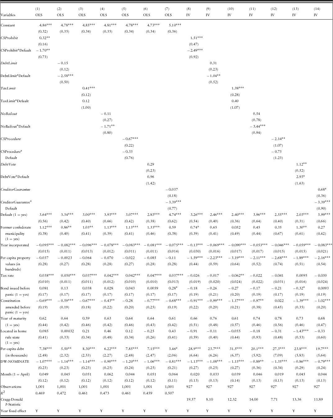
Finally, Table 7 provides the results for equation (3), which interacted each of the constitutional variables with whether or not a municipality defaulted.
Constitutional variable interactions OLS and IV results dependent variable = average yield to maturity
Robust standard errors in parentheses.
***p < 0.01; **p < 0.05; *p < 0.1.
Columns 1–7 provide the OLS results while columns 8–14 give the instrumental variable results. The results are most consistent between the OLS and instrumental variable specifications. These results also shed light on how much borrowing costs were affected by each of these constitutional budget rules depending on whether or not a municipality had defaulted.
Specifically for the variables CSProhibit, DebtLimit, NoBailout, and CreditorGuarantee, the findings suggest that each of these led to much lower borrowing costs for a defaulting municipality once they were imposed. Specifically, between the OLS and instrumental variable estimates, CSProhibit reduced borrowing costs on a municipality which had defaulted between 170 and 249 basis points, while DebtLimit reduced those costs between 358 and 104 basis points, NoBailout between 171 and 344 basis points, and CreditorGuarantee at 339 basis points. Furthermore, both TaxLimit and DebtVote variables increased borrowing costs, but with little statistical significance. Finally, CSProcedure also lowered borrowing costs, but was not statistically significant and the magnitude of the coefficient was much smaller relative to the more binding constitutional constraints.
Overall, these outcomes, especially from equation (3), would suggest that more binding constraints and outright prohibitions on specific behavior had a much more profound impact on overall borrowing costs than did procedural safeguards. This would especially appear to be the case for those municipalities that defaulted on their obligations relative to those that did not.
For debt prohibitions, it would seem to suggest that by prohibiting municipalities from increasing debt above a certain percentage of the assessed value of real property, it meant that those same municipalities would presumably be able to repay that same debt in a much timelier manner. Most interesting are the interaction results, and the impact that debt limits had on defaulting city government's through time. Ultimately it would appear that the most significant way for a municipal government to recommit after default was through the imposition of strict limits on behavior rather than procedural safeguards against it.
In regard to the results for constitutional tax limits, Hillhouse (Reference Hillhouse1936) noted that the strict tax limits that were imposed had a two-fold unintended consequence. First, some of the more financially sound cities became unable to meet their debt obligations as doing so would have resulted in tax obligations above the mandated limit. Second, these limits many times made it even more difficult for creditors to find legal recourse, as executing a court-ordered writ of mandamus to force tax collection in order to repay creditors also would have required tax obligations to increase above the legal limit.
Finally, the results associated with hard budget constraints might suggest that markets understood the potential moral hazard that may be created if a state were to assume the debts of its municipalities. Specifically, by assuming such debt a state may increase its own risk of default or possibly even repudiation. Such a policy may have further created the incentive for municipalities to undertake still riskier behavior and investments in the future. Furthermore, by imposing such a limit it may have signaled to credit markets a serious commitment by state governments to much sounder fiscal policy in general as compared to other states.
Discussion
Overall, these results provide some potentially interesting implications for municipal governments today. For instance, a large body of literature has developed regarding the importance of hard budget constraints within a system of federalism (Goodspeed, Reference Goodspeed2002; Qian and Roland, Reference Qian and Roland1998; Weingast, Reference Weingast1995). This is especially true within the United States today, where due to the recent financial crisis, new calls have been made and considerations put forth to bailout junior level governments. Detroit became the most recent city to be considered for $500 million in long-term debt assistance in order to overcome its own fiscal woes (Detroit Growth and Stability Act of 2012, H.R. 4308). There has also been an active effort to acquire similar relief through the state government (The Economist Magazine 7th April 2012). However, just as much of the literature has suggested, through hard budget constraints it is possible to check the moral hazard problem associated with those bailouts and to force a lower level government to pursue more fiscally sound and time-consistent policy. From the above analysis, this would appear to have been translated into lower average yields (and thus lower borrowing costs), for municipalities that faced that constraint. This is also true of stricter debt limits and repayment requirements. Even today many of these requirements still remain in state constitutions at least in some form. However, these constraints have slowly evolved over time.
An important aspect to this evolutionary process was the creation of special assessment and taxing districts. These districts largely developed through court interpretation of a number of these constitutional restrictions and enhanced a municipality's ability to better target local infrastructure to locations and individuals who had the greatest demand for them and also, presumably, the greatest willingness to pay (Wallis and Weingast, Reference Wallis, Weingast, Garrett, Graddy and Jackson2008). Thus, this greater flexibility allowed municipalities to better match both the direct beneficiaries of those public projects and to better target public funding of those activities, while also divesting many of those municipalities of some of the liability associated with such financing. Of course, these reflections and other possible implications are still in need of much more future research.
5. Conclusion
Fiscal difficulties at the municipal level are not a new phenomenon, especially in the United States. In fact, the first episode of large-scale municipal fiscal problems and default occurred as a direct result of the panic of 1873 and ensuing depression. The aftermath of this panic resulted in multitudes of municipalities, with outstanding obligations totaling between $100 and $150 million, defaulting. This episode led to upheaval across state and local governments, whereby numerous states passed constitutional amendments meant to directly curtail municipalities from pursuing similar policy in the future.
This study attempted to empirically analyze the impact that these constitutional constraints had on municipal borrowing costs in the wake of these constitutional changes. Overall, the results of this paper suggest that markets were indeed both receptive and perceptive in regard to the significance of these constitutional amendments. The majority of those constraints that were passed by states did lead to definite action by market participants. However, most interesting is the way in which markets reacted to the type of constraint imposed. Specifically, binding repayment requirements and debt limits, as well as hard budget constraints generally led to much lower borrowing costs for municipal governments (especially after defaulting) than did less restrictive, procedural safeguards against similar behavior.
This adds an additional twist to the impact that constitutionally constraining government from pursuing suboptimal and time-inconsistent policy had on public finance and fiscal obligations. Furthermore, it helps to better understand how markets reacted to these constraints through time. Finally, it also provides an understanding of the importance of finding optimal constraints that will create time-consistent policy, and which will lead to robust institutional arrangements that are better able to withstand the impact of market shocks and fiscal crises as they emerge.
Description of constitutional rules and their shorthand name
Municipal bond issues by date and city
First stage results for instrumental variables