1. Introduction
Macroeconomic theoretical models have increasingly incorporated the formation of household consumption habits. In particular, standard medium-scale dynamic stochastic general equilibrium (DSGE) models often employ habit formation in household consumption to reproduce the hump-shaped dynamics of endogenous variables in response to structural shocks (Christiano et al. Reference Christiano, Eichenbaum and Evans2005; Smets and Wouters Reference Smets and Wouters2007).
Ravn et al. (Reference Ravn, Schmitt-Grohé and Uribe2006) recently extended the concept of habit formation to “deep habits,” a form that inherits the empirically desirable hump-shaped dynamics.Footnote 1 Traditional (or “superficial”) habits are formed for aggregated goods, while deep habits are formed for goods-by-goods.Footnote 2 Deep habits generate additional externalities in models, providing new insights. For example, Ravn et al. (Reference Ravn, Schmitt-Grohé and Uribe2006) highlighted that deep habits change the demand structure of households; therefore, price setting decisions of final-goods firms and markups of the goods price over their cost could also be altered, bringing crowding-in effects of fiscal policy (Ravn et al. Reference Ravn, Schmitt-Grohé and Uribe2006; Zubairy Reference Zubairy2014).Footnote 3 Many previous studies focused on the role of deep habits in fiscal policy; however, only a few considered the role of deep habits in optimal monetary policy. In particular, to the best of our knowledge, no open economy NK models with deep habits have considered the optimal monetary policy.
This study develops a two-country NK model with deep habits in household consumption, extending Leith et al. (Reference Leith, Moldovan and Rossi2012, Reference Leith, Moldovan and Rossi2015)’s closed economy NK model with deep habits to a two-country version based on Corsetti et al. (Reference Corsetti, Dedola, Leduc, Corsetti, Dedola and Leduc2010), Ravn et al. (Reference Ravn, Schmitt-Grohe and Uribe2007), Jacob and Uusküla (Reference Jacob and Uusküla2019), and Ida and Okano (Reference Ida and Okano2023a). We then examine the central bank’s behavior in solving the Ramsey problem, which maximizes both countries’ economic welfare in a coordinated fashion. Furthermore, we compare cooperative and noncooperative policies to examine the welfare gains from international coordination.
In a two-country model, the central bank should consider the terms of trade externality and consumption externality due to deep habit. When terms of trade externalities exist—for instance, high elasticity of substitution between domestic and foreign goods—improving the terms of trade can increase imported-goods consumption while reducing the domestic labor burden, thereby improving economic welfare (Pappa Reference Pappa2004; De Paoli Reference De Paoli2009). Therefore, in conducting monetary policy to maximize economic welfare, the central bank must balance consumption externalities arising from deep habits, terms of trade externalities, and the costs associated with nominal rigidities.
Our main findings are as follows. Unlike in the standard NK model, when a deep habit exists, the central bank faces a trade-off between the output gap and inflation stability even in response to a productivity shock. Previous studies have shown that when the central bank conducts the optimal commitment policy, it is more reluctant to move the interest rate aggressively in a closed economy model with deep habits than a model without deep habits. Moreover, unlike in a closed economy, the central bank alters the interest rate more in the two-country open economy model. The key to understanding this finding lies in the asymmetric changes in domestic and foreign markups generated by the deep habits and the resulting changes in relative demand. Combining these changes with the central bank’s behavior and the externalities of the terms of trade that are unique to the open economy model leads to markedly different results from those of a closed economy. In an open economy, regardless of deep habits, the central bank is incentivized to internalize the externalities due to the terms of trade. When deep habits exist, the process of habit formation, along with the counter-cyclical markup behavior, introduces a price-inelastic component into the demand function for individual goods. This inelasticity strengthens the incentive to influence the terms of trade, enhancing the central bank’s interest rate movements; however, if the home bias in favor of domestic goods is small, the international spillover effects of economic shocks become increasingly pronounced. Thus, the necessity to adjust the terms of trade diminishes, leading to a more moderate response of interest rates.
We also show that the deviations from the law of one price (LOP), or the good-specific real exchange rate, generated by the deep habits are related to the degree of home bias. In particular, the deviations fully disappear without a home bias.
Comparing welfare gains shows that the welfare gains from coordination depend on key structural factors such as price rigidity, deep habits, and home bias. When prices are flexible, coordination benefits are relatively small; however, as price rigidity increases, the gains from coordination become more significant as noncooperative policies fail to adjust prices optimally. Deep habits tend to reduce coordination benefits by naturally smoothing international consumption imbalances.
Impulse response analysis further reveals how policy coordination affects macroeconomic dynamics. Under cooperative policies, interest rate adjustments help stabilize domestic output and inflation at the cost of slightly increasing foreign volatility. This situation suggests that policy coordination can internalize the externalities arising from terms of trade and consumption habit formation.
The remainder of the paper is organized as follows. Section 2 reviews the related literature, Section 3 describes the model structure, and Section 4 describes the central bank’s optimal monetary policy. Section 5 demonstrates the impulse responses to the structural shocks, calculates the welfare gains from international policy coordination, and provides economic intuition about the results. Finally, Section 6 concludes our research and summarizes the results.
2. Literature review
Our study is based on two research strands: deep consumption habits and international monetary-policy coordination.
Many fields have used habit formation to generate real rigidity. For instance, Abel (Reference Abel1990) incorporated the “keeping up with the Joneses effect” in the utility function into the asset pricing model to examine the equity premium puzzle. Previous studies noted the similarities between deep habits and the customer market model (Bils Reference Bils1989), as deep habits modify demand behavior at the goods-by-goods level, affecting firm-level pricing like customer markets.Footnote 4
Incorporating deep habits into the NK model has drawn attention to how deep habits produce countercyclical markup. In other words, under the deep habit, firms may respond to an increase in current demand by lowering markups and reducing prices to secure future profits. Thus, “price may magnify, rather than stabilize, demand movements” (Bils Reference Bils1989). The influence of countercyclical markups on optimal monetary policy is significant. As Leith et al. (Reference Leith, Moldovan and Rossi2012) discussed, under a deep habit, the central bank cannot lower interest rates sufficiently even when they should (e.g., due to positive productivity shocks). This situation occurs because lowering the interest rate will cause firms to lower their markups, leading to undesirable overconsumption. The dilemma that lowering interest rates to stimulate demand also impacts the supply side generates a trade-off between inflation stability and the output gap, indicating a deviation from the “divine coincidence.” In the context of optimal policy, Amato and Laubach (Reference Amato and Laubach2004) investigated the optimal monetary policy under internal superficial habit in consumption. Givens (Reference Givens2016) explored how deep habits affect welfare gains from commitment relative to discretion, revealing that deep habits weaken the stabilization trade-offs facing a discretionary planner.
Some properties from countercyclical markup may carry over in the two-country model; however, which properties and the extent to which they are inherited in the open economy model are worth investigating. For example, deep habits can affect international price markups. Specifically, Ravn et al. (Reference Ravn, Schmitt-Grohe and Uribe2007) showed that deep habits could endogenously generate deviations from the LOP. Furthermore, Jacob and Uusküla (Reference Jacob and Uusküla2019) showed that deep habits could be the source of incomplete pass-through of exchange rates to international prices.
This paper also considers optimal monetary policy in an open economy model since it incorporates deep habits into a two-country open economy model. An intriguing question for optimal monetary policy in an open economy model is whether each country gains more by coordinating its policies than by pursuing its welfare without cooperation (cooperation vs. noncooperation). There have been many previous studies in this regard; they can be divided by the export pricing behavior of firms: producer currency pricing (PCP) vs. local currency pricing (LCP). PCP models dealing with international cooperation are, for example, Clarida et al. (Reference Clarida, Galí and Gertler2002); Benigno and Benigno (Reference Benigno and Benigno2006); Pappa (Reference Pappa2004) and Obstfeld and Rogoff (Reference Obstfeld and Rogoff2002). LCP models include Devereux and Engel (Reference Devereux and Engel2003) and Engel (Reference Engel2011), Fujiwara and Wang (Reference Fujiwara and Wang2017).Footnote 5 Moreover, De Paoli (Reference De Paoli2009); Corsetti and Dedola (Reference Corsetti and Dedola2005); Corsetti et al. (Reference Corsetti, Dedola, Leduc, Corsetti, Dedola and Leduc2010) provide a comprehensive discussion of the economy’s behavior and optimal monetary policy in PCP and LCP.
Similar conclusions regarding policy coordination gains are obtained for PCP and LCP; policy coordination gains can be generated, but they are not large.Footnote 6 Regarding PCP, Clarida et al. (Reference Clarida, Galí and Gertler2002) pointed out that the nominal exchange rate is important in a relative price adjustment, meaning that distortions can occur when countries strategically manipulate exchange rates or terms of trade in favor of each other’s economy. There is room for policy coordination to eliminate these distortions. Engel (Reference Engel2011) argued that in the case of LCP, nominal exchange rates are no longer helpful for the relative price adjustment; instead, coordination gains are generated by coordinately correcting deviations from the LOP and currency misalignments. Kim (Reference Kim2023), on the other hand, constructs an asymmetric two-country model. One country follows the PCP, and the other follows the LCP. In this case, the asymmetry of the model allows for a not-too-small level of coordinated gains even under conditions where gains would disappear in both the PCP and LCP models.
These models are related to this paper, but no models listed include deep habit. This paper gains new findings by introducing deep habit. The main questions are about how deep habits affect gains and the relationship between home bias and deep habit. Both home bias and deep habits are related to household preferences; however, their interaction has not yet been examined, and it is particularly interesting. We develop the two-country model based on Corsetti et al. (Reference Corsetti, Dedola, Leduc, Corsetti, Dedola and Leduc2010),Footnote 7 incorporating deep habits in consumption similarly to Ravn et al. (Reference Ravn, Schmitt-Grohe and Uribe2007); Jacob and Uusküla (Reference Jacob and Uusküla2019). Our two-country model allows for different pricing between domestic and foreign markets by reflecting distinct consumption habits at the individual goods level. Therefore, it can reproduce the deviation from the LOP as in Ravn et al. (Reference Ravn, Schmitt-Grohe and Uribe2007). We investigate the optimal commitment policy following Leith et al. (Reference Leith, Moldovan and Rossi2012, Reference Leith, Moldovan and Rossi2015).
3. The model
We develop the two-country model based on Bodenstein, et al. (Reference Bodenstein, Guerrieri and LaBriola2019), incorporating deep habits in consumption following Ravn et al. (Reference Ravn, Schmitt-Grohe and Uribe2007); Jacob and Uusküla (Reference Jacob and Uusküla2019)Footnote 8 and discuss optimal monetary policies following Leith et al. (Reference Leith, Moldovan and Rossi2012, Reference Leith, Moldovan and Rossi2015).
The two countries are symmetrical and the same size. Home and foreign households consume home-produced and foreign-produced goods with home bias and deep habit. Final goods producers maximize profits in monopolistically competitive domestic and foreign markets. Intermediate goods producers produce input for domestic final goods producers with monopolistic competition. The government levies a lump-sum tax on households and subsidizes firms to eliminate distortions from monopolistic competition and deep consumption habits in a steady state. Central banks maximize social welfare cooperatively or noncooperatively, using each domestic inflation as a policy instrument. The model structure of the foreign country is symmetrical to that of the home country. Unless otherwise noted, we denote foreign variables with an asterisk.
We should consider external habit (Smets and Wouters Reference Smets and Wouters2007) rather than internal habit formation (Fuhrer Reference Fuhrer2000; Christiano et al. Reference Christiano, Eichenbaum and Evans2005). Households with external habits cannot internalize the externalities of their utility on other households’ utility because they care about other households’ consumption rather than their past consumption (“keeping up with the Joneses” effect.)Footnote 9
3.1. Households
Households derive utility from the consumption of home and foreign goods, and they form consumption habits at the level of individual goods rather than aggregate goods. When habits are deep, consumer preferences are at the individual goods level over time, generating the habit-persistence at a goods-by-goods level (Jacob and Uusküla Reference Jacob and Uusküla2019).
A representative household
 $k \in [0, 1]$
maximizes lifetime utility for an infinite period.
 \begin{align} E_{0}\sum ^{\infty }_{t=0} \beta ^{t} \left [ \frac { \left ( X_{t}^{k} \right )^{1-\sigma } } {1-\sigma } - \chi \frac { \left ( N_{t}^{k} \right )^{1+\upsilon } } {1+\upsilon } \right ] \end{align}
where
 $X_t$
is the habit-adjusted aggregate consumption of the household.
 $N_t$
represents hours worked, and
 $\beta$
is the discount factor.
 $\sigma$
denotes the inverse of the intertemporal elasticities of habit-adjusted consumption,
 $\upsilon$
is the inverse of the intertemporal elasticities of work, and
 $\chi$
is the relative weight on disutility from time spent working.
 $X_t^k$
is a CES composite of habit-adjusted consumption of domestic
 $X_{D, t}^k$
and imported goods
 $X_{M, t}^k$
:
 \begin{align} X_{t}^k & = \left ( \omega ^{\frac {1}{\eta }} \left(X_{D, t}^k\right)^{\frac {\eta -1}{\eta }} + (1-\omega )^{\frac {1}{\eta }} \left(X_{M,t}^k\right)^{\frac {\eta -1}{\eta }} \right )^{\frac {\eta }{\eta -1}} \end{align}
where
 $\eta$
is the elasticity of substitution between domestic and imported goods and
 $\omega \in [0, 1]$
is a degree of home bias in consumption.
 $X_{D, t}^k$
and
 $X_{M, t}^k$
are also CES aggregates of the variety of goods
 $i \in [0, 1]$
:
 \begin{align} X_{D,t}^k & = \left [ \int _0^1 ( C_{D,t}^k(i) - \theta _{D} \bar S_{D, t-1}(i) )^{\frac {\epsilon -1}{\epsilon }} di \right ]^{\frac {\epsilon }{\epsilon -1}}, \end{align}
 \begin{align} X_{M,t}^k & = \left [ \int _0^1 ( C_{M,t}^k(i) - \theta _{M} \bar S_{M,t-1}(i) )^{\frac {\epsilon -1}{\epsilon }} di \right ]^{\frac {\epsilon }{\epsilon -1}} \end{align}
where
 $\epsilon$
is the elasticity of substitution among the variety of goods, and
 $\bar S_{D, t}$
and
 $\bar S_{M, t}$
are the stocks of consumption habits.
Habit stocks are the sum of stocks at the end of the last period and habits that will be newly formed in the current period. The law of motions for habit stocks is given by:
 \begin{align} \bar S_{D,t}(i) & = \varrho _{D} \bar S_{D, t-1} (i) + (1 - \varrho _D) \bar C_{D, t}(i), \end{align}
 \begin{align} \bar S_{M,t}(i) & = \varrho _{M} \bar S_{M, t-1}(i) + (1 - \varrho _M) \bar C_{M, t}(i). \end{align}
Note that habit stocks are independent of each household
 $k$
.
 $\bar C_{D, t}(i) = \int _0^1 C_{D, t}^k(i) dk$
and
 $\bar C_{M, t}(i) = \int _0^1 C_{D, t}^k(i) dk$
are the average consumption of domestic goods and imported goods, respectively. In each period, household
 $k$
refers to the stock of the average household consumption in the previous period concerning good
 $i$
and allocates a portion of it to habit formation. Note that habitual consumption stocks do not yield utility by definition.
Demand functions consist of a price-elastic component and an inelastic component due to the stock of habit consumption. The demand functions of domestic and imported goods for each good
 $i$
are described as follows:
 \begin{align} C_{D,t}^k(i) & = \left ( \frac {P_{D,t}(i)} {P_{D,t}} \right )^{-\epsilon } X_{D,t}^k + \theta _{D} \bar S_{D,t-1}(i), \end{align}
 \begin{align} C_{M,t}^k(i) & = \left ( \frac {P_{M,t}(i)} {P_{M,t}} \right )^{-\epsilon } X_{M,t}^k + \theta _{M} \bar S_{M,t-1}(i) \end{align}
where
 $P_{D, t}(i)$
and
 $P_{M, t}(i)$
are price of domestic goods
 $i$
and price of imported goods
 $i$
, respectively.
 $P_{D, t}$
and
 $P_{M, t}$
are the aggregate price of domestic goods and imported goods, respectively:
 \begin{align} P_{D,t} & = \left ( \int ^1_0 P_{D,t}^{1-\epsilon }(i) di \right )^{\frac {1}{1-\epsilon }}, \end{align}
 \begin{align} P_{M,t} & = \left ( \int ^1_0 P_{M,t}^{1-\epsilon }(i) di \right )^{\frac {1}{1-\epsilon }}. \end{align}
The budget constraint for household
 $k$
is as follows:
 \begin{align*} \int ^1_0 \left [ P_{D,t}(i) C_{D,t}^k(i) + P_{M,t}(i) C_{M,t}^k(i) \right ] di + E_t \left \{ Q_{t, t+1} D_{t+1}^k \right \} \leq D_t^k + W_t N_t^k + \Phi _t - T_t \end{align*}
where
 $W_t$
is the nominal wage, and
 $D_{t}$
is the nominal payoff on the portfolio of assets.
 $Q_{t, t+1}$
is the one-period stochastic discount factor for nominal payoffs relevant to the domestic household, and
 $E_t$
is the mathematical expectation conditional on information available at time
 $t.$
Following Clarida et al. (Reference Clarida, Galí and Gertler2002), we assume households have free access to a complete set of contingent claims traded internationally.
 $\Phi _t$
is the dividend from firms owned by households and
 $T_t$
is lump-sum tax (if
 $T_t \geq 0$
) or subsidy (if
 $T_t \lt 0.$
)
 \begin{align} P_{D,t} X_{D,t}^k + P_{M,t} X_{M,t}^k + \bar v_{t} + E_t \left \{ Q_{t, t+1} D_{t+1}^k \right \} \leq D_t^k + W_t N_t^k + \Phi _t - T_t \end{align}
and
 \begin{align} \bar v_{t} = \theta _{D} \int ^1_0 P_{D,t}(i) \bar S_{D,t-1}(i) di + \theta _{M} \int ^1_0 P_{M,t}(i) \bar S_{M,t-1}(i) di \end{align}
where
 $\bar v_t$
is the expenditure on the stock of habitual consumption. Note that from Equations (5) and (6),
 $\bar v_t$
include past average consumptions. Due to the term
 $\bar v_t$
, the budget constraint includes consumption externality since average consumptions are given for each household
 $k$
.
Households maximize lifetime utility (1) subject to its budget constraint (11). The first-order condition, concerning habit-adjusted domestic consumption
 $X_{D, t}$
, can be defined as follows:
 \begin{align} \beta E_t \left [ \left ( \frac {X_{t+1}}{X_t} \right ) ^{-\sigma +1/\eta } \left ( \frac {X_{D, t+1}}{X_{D, t}} \right ) ^{-1/\eta } \left ( \frac {P_{D, t}}{P_{D, t+1}} \right ) \right ] R_t = 1 \end{align}
where
 $R_t \equiv 1 / E_t\{Q_{t, t+1}\}$
denotes the risk-free gross nominal interest rate between periods
 $t$
and
 $t+1$
. The superscript
 $k$
can be dropped in the optimal conditions due to the assumption of homogeneity of the representative households. The form of consumption Euler equation (13) is equivalent to that under traditional (or superficial) habit formation.
The first-order condition for hours worked is:
 \begin{align} (X_{t})^{\sigma } \left [ \omega ^{1/\eta } \left ( \frac {X_{D, t}} {X_t} \right ) ^{-1/\eta } \right ] ^{-1} \chi (N_t)^{\upsilon } = \frac {W_t}{P_{D,t}}. \end{align}
We can combine the first-order conditions for
 $X_{D, t}$
and
 $X_{M, t}$
to derive the following condition:
 \begin{align} & \left ( \frac {\omega } {1-\omega } \right ) ^{1/\eta } \left ( \frac {X_{D, t}} {X_{M, t}} \right ) ^{-1/\eta } = \frac {P_{D,t}}{P_{M, t}}. \end{align}
3.2. Final goods producers
Final-goods firms produce final goods by aggregating intermediate goods. We assume that final goods producers can flexibly change goods’ prices and can make different pricing decisions for home and foreign markets. We also assume that domestic final-goods firms only purchase the intermediate goods produced in their home country. The final-goods firms face monopolistic competition and determine the optimal price and markups conditional on the demand function of each good. Note that the deep habit affects the demand function, as shown in (7). Unlike the standard NK model, the model with deep habits has a demand function that includes the term independent of the current price. This additional term implies that the demand function depends on the past average (or external) demand. In other words, the current pricing behavior of final goods producers can affect current and future expected demands and profits, called the intertemporal effect of a deep habit (Ravn et al. Reference Ravn, Schmitt-Grohé and Uribe2006).
Each firm produces final goods
 $Y(i)$
by CES-aggregating intermediate goods
 $Y(i, j)$
:
 \begin{align} Y_t(i) & = \left ( \int ^1_0 Y_t (i,j)^{\frac {\xi -1}{\xi }} dj \right ) ^{\frac {\xi }{\xi -1}}. \end{align}
Then, the final goods are shipped to the home and foreign markets.
 \begin{align} Y_t(i) & = Y^D_{t}(i) + Y^{EX}_{t}(i) \end{align}
where
 $Y^{D}_{t}(i)$
is the domestic output provided to domestic consumers, and
 $Y^{EX}_{t}(i)$
is an exported output. Thus, the market-clearing condition of domestic output is
 \begin{align} Y^D_{t}(i) & = C_{D,t}(i), \end{align}
 \begin{align} Y^{EX}_{t}(i) & = C_{M,t}^{*}(i). \end{align}
Where
 $C_{M,t}^*(i)$
is the consumption of foreign households for the final goods
 $i$
produced in the home country. Hereafter, foreign variables are denoted by a superscript
 $*$
.
3.2.1. Profit maximization for final-goods firms
The profits of final goods firms in our model would be nonzero since the demand function has a constant term independent of its price. We define the profit of a final goods firm as follows:
 \begin{align} \Phi _t (i) & \equiv \Phi _{D, t}(i) + \Phi _{M, t}^*(i),\\[-9pt]\nonumber \end{align}
 \begin{align} \Phi _{D, t}(i) & \equiv \left ( P_{D,t}(i) - P_{t}^{m}(i) \right ) C_{D, t}(i),\\[-9pt]\nonumber \end{align}
 \begin{align} \Phi _{M, t}^{*}(i) & \equiv \left ( \mathcal{E}_t P_{M,t}^*(i) - P_{t}^{m}(i) \right ) C_{M, t}^{*}(i)\\[-9pt]\nonumber \end{align}
where
 $\Phi (i)$
is the total profit of the final good firm
 $i$
,
 $\Phi _D (i)$
is the profit from domestic sales, and
 $\Phi _M^* (i)$
is the profit from sales to foreign households.
 $P_t^m(i)$
is the price index of intermediate goods for producing final goods
 $i$
.
When households have deep habits in consumption, demand for goods may differ, and firms would differentiate prices in domestic and foreign markets. Ravn et al. (Reference Ravn, Schmitt-Grohe and Uribe2007) named this “pricing to habits,” showing that deviations from the LOP occur endogenously.Footnote 10 Thus, as described in Section 2, our model can be regarded as a sort of LCP.Footnote 11
3.2.2 .Optimal price setting of final goods for domestic consumption
Final goods firms maximize the discounted present value of future domestic sales profits as follows:
 \begin{align} & \max _{ \left \{ P_{D, t}(i) ,C_{D, t}(i) \right \} } E_{t} \sum ^{\infty }_{s=0} Q_{t,t+S} \left ( P_{D,t+S}(i) - P_{t+S}^{m}(i) \right ) C_{D, t+S}(i) \end{align}
subject to the demand function (7) and the law of motion of the habit stock (5):
 \begin{align} C_{D,t+s}(i) & = \left ( \frac {P_{D, t+s}(i)}{P_{D, t+s}} \right )^{-\epsilon } X_{D,t+s} + \theta _D C_{D, t+s-1}(i) \end{align}
where
 $\varrho _D = 0$
for simplicity. We derive the first-order conditions of this problem as follows:
 \begin{align} \Lambda _{D, t}(i) & = \left ( P_{D, t}(i) - P_{t}^{m}(i) \right ) + \theta _D E_{t} \left [ Q _{t,t+1} \Lambda _{D, t+1} (i) \right ], \end{align}
 \begin{align} C_{D, t}(i) & = \Lambda _{D, t}(i) \left [ \epsilon \left ( \frac {P_{D,t}(i) }{P_{D,t}} \right ) ^{-\epsilon -1} (P_{D,t})^{-1} X_{D,t} \right ] \end{align}
where
 $\Lambda _{t, D} (i)$
is the Lagrange multiplier.
3.2.3 Optimal price settings for exports
Similarly, we set up the profit maximization problem for exported goods toward the foreign country,
 $Y_{t}^{EX}=C_{M, t}^*$
,
 \begin{align} \max _{ \left \{ \mathcal{E}_t P_{M, t}^*(i) ,C_{M,t}^{*}(i) \right \} } E_{t}\sum ^{\infty }_{s=0}Q_{t,t+s} \left ( \mathcal{E}_t P_{M,t+s}^*(i) -P_{t+s}^{m}(i) \right ) C_{M, t+s}^{*}(i) \end{align}
subject to the demand function
 \begin{align} C_{M, t+s}^{*}(i) & = \left ( \frac {P_{M, t+s}^*(i)}{P_{M, t+s}^*} \right )^{-\epsilon } X_{M,t+s}^* + \theta _{M}^{*} C_{M, t+s-1}^*(i). \end{align}
Note that
 $P_{t+s}^m (i)$
is as given when intermediate firms optimize their goods price.
Domestic firms choose the final-goods price in terms of home currency
 $\mathcal{E}_t P^*_{M}(i)$
; conversely, foreign households determine their consumption behavior in terms of foreign currencies. Moreover, foreign households may have different consumption habits or preferences for identical goods from those in the home country.
The following are this problem’s first-order conditions:
 \begin{align} \Lambda _{M, t}^{*}(i) & = \left ( \mathcal{E}_t P_{M, t}^*(i) - P_{t}^{m}(i) \right ) + \theta _M^{*} E_{t} \left [ Q _{t,t+1} \Lambda _{M, t+1}^* (i) \right ] \end{align}
 \begin{align} C_{M, t}^{*}(i) & = \Lambda _{M, t}^{*}(i) \left [ \epsilon \left ( \frac {P_{M,t}^*(i)}{P_{M,t}^*} \right ) ^{-\epsilon -1} \left ( \mathcal{E}_t P_{M,t}^* \right ) ^{-1} X_{M,t}^* \right ]. \end{align}
3.3. Intermediate goods producers
Following Leith et al. (Reference Leith, Moldovan and Rossi2012, Reference Leith, Moldovan and Rossi2015), the intermediate goods firms facing monopolistic competition derive the marginal cost function by solving the cost minimization problem and determining the optimal price under nominal price rigidity.
NK models incorporating deep habits often adopt Rotemberg (Reference Rotemberg1982)-type adjustment cost instead of Calvo pricing as price stickiness for aggregation convenience. Whether Rotemberg-type or Calvo (Reference Calvo1983)-type price stickiness, the same Phillips curve can be obtained up to a first-order approximation (Woodford Reference Woodford2003a). Conversely, Lombardo and Vestin (Reference Lombardo and Vestin2008) showed that the two pricing assumptions could yield different social inflation costs when the steady-state is inefficient. Considering this difference, we choose the Calvo pricing as a source of price stickiness by following Leith et al. (Reference Leith, Moldovan and Rossi2009). Specifically, we deal with these two rigidities separately: intermediate goods firms face Calvo-type nominal rigidities, whereas final goods firms’ demand functions are affected by households’ deep habits. In such a way, as suggested by Leith et al. (Reference Leith, Moldovan and Rossi2009), the model can be built with Calvo pricing and deep habits without losing its desirable aggregate properties.
3.3.1. Production function of intermediate goods firms
The production function of the intermediate firm
 $j$
that produces the intermediate good used for inputs in final goods
 $i$
,
 $Y(i, j)$
, is defined as follows:
 \begin{align} Y_{t}(i,j) = A_t N_{t} (i,j) \end{align}
where
 $A_t$
is an exogenous technological progress that is common to individual intermediate goods firms. The (log-linearized) technology follows AR(1):
 $\ln A_t = \rho _a \ln A_{t-1} + \epsilon _t^a$
where
 $\rho _a \in (0, 1)$
is the coefficient, and
 $\epsilon _t^a$
is independent and identically distributed productivity shock.
From the cost minimization problem for intermediate goods firms, we derive
 $MC_t = (1-\tau ) W_t/A_t$
where
 $MC_t$
is a nominal marginal cost common across firms.
 $\tau$
is the tax rate imposed on nominal costs chosen to achieve an efficient allocation at the steady-state equilibrium.Footnote
12
Under monopolistic competition, intermediate goods firms face the following demand function:
 \begin{align} Y_t(i,j) & = \left ( \frac {P_t^m(i,j)}{P_t^m(i)} \right )^{-\xi } Y_t(i) \end{align}
and
 \begin{align} P_t^m(i) \equiv \left ( \int ^1_0 (P_t^m)^{1-\xi }(i,j) dj \right ) ^{\frac {1}{1-\xi }} \end{align}
where
 $P_t^m(i,j)$
is the price of the intermediate good
 $j$
put into the final good
 $i$
.
 $P_t^m(i)$
is the price index of the intermediate goods in terms of the final good
 $i$
. We assume intermediate goods
 $Y_t(i,j)$
are provided only domestically and not traded internationally; thus, intermediate firms do not differentiate their prices between home and foreign countries.
3.3.2. Optimal price setting of intermediate goods firms
The intermediate goods firm maximizes the discounted sum of profit in the face of Calvo (Reference Calvo1983)-type nominal price rigidity. The nominal profit of the intermediate goods firm is defined as
 $\Phi ^m_t (i, j) \equiv (P^{m}_t(i, j) - MC_t) Y_t (i, j)$
. The profit maximization problem of the intermediate goods firm is as follows:
 \begin{align*} \max _{ P_{t}^{mo}(i, j) } E_{t} \sum ^{\infty }_{s=0} \alpha ^{s} Q_{t,t+s}(P_{t}^{mo}(i, j) - MC_{t+s}) Y_{t+s} (i, j) \end{align*}
subject to the demand function for the intermediate goods (32):
 \begin{align} \quad Y_{t+s}(i,j) & = \left ( \frac {P_{t}^{mo}(i,j)}{P_{t+s}^{m}(i)} \right )^{-\xi } Y_{t+s} (i) \end{align}
where
 $\alpha$
is the degree of price stickiness, and
 $P^{mo}_{t}(i, j)$
is optimal price of intermediate goods
 $j$
for final goods
 $i$
.
The first-order condition is as follows:
 \begin{align} \frac {P_{t}^{mo}(i, j)}{P_{D, t}} = \left ( \frac {\zeta _t}{\zeta _t -1} \right ) \frac { E_{t} \sum ^{\infty }_{s=0} (\alpha \beta )^{s} X_{t+s}^{-\sigma +1/\eta } X_{D, t+s}^{-1/\eta } mc_{t+s} \left ( P_{t+s}^{m}(i) \right )^{\xi } Y_{t+s}(i) }{ E_{t} \sum ^{\infty }_{s=0} (\alpha \beta )^{s} X_{t+s}^{-\sigma +1 / \eta } X_{D, t+s}^{-1/\eta } \left ( \frac {P_{D, t+s}}{P_{D, t}} \right )^{-1} \left ( P_{t+s}^{m}(i) \right )^{\xi } Y_{t+s}(i) } \end{align}
where
 $mc_t \equiv MC_t / P_{D, t}$
is the real marginal cost in terms of domestic prices, and
 $\zeta _t$
is the time-varying elasticity of substitution between intermediate goods.
 $\zeta _t / (\zeta _t -1)$
implies the desired markup of the intermediate goods firms. We assume that
 $\zeta _t$
follows AR(1) process:
 $\ln \zeta _{t}=\left ( 1- \rho _m\right ) \ln \xi +\rho _{m}\zeta _{t-1}+\varepsilon _{t}^{m}$
. An exogenous increase in
 $\zeta _t$
implies a reduction in the desired markup of intermediate goods producers, interpreted as a negative cost-push shock on the supply side.Footnote
13
(35) can be rewritten using the auxiliary variables
 $K_{1, t}, K_{2, t}$
as follows:
 \begin{align} \frac {P_{t}^{mo}(i,j)}{P_{D,t}} = \left (\frac {\zeta _{t}}{\zeta _t -1}\right )\frac {K_{1, t}}{K_{2,t}} \end{align}
where
 \begin{align*} K_{1, t} & \equiv E_{t}\sum ^{\infty }_{s=0}(\alpha \beta )^{s} X_{t+s}^{-\sigma +1/\eta } X_{D, t+s}^{-1/\eta } mc_{t+s} \left ( \frac {P_{t+s}^{m}(i)}{P_{D,t}} \right )^{\xi } Y_{t+s}(i), \\ K_{2, t} & \equiv E_{t}\sum ^{\infty }_{s=0} (\alpha \beta )^{s} X_{t+s}^{-\sigma +1/\eta } X_{D, t+s}^{-1/\eta } \left ( \frac {P_{D, t+s}}{P_{D, t}} \right )^{-1} \left ( \frac {P_{t+s}^{m}(i)}{P_{D,t}} \right )^{\xi } Y_{t+s}(i). \end{align*}
By transforming these into recursive forms, we get
 \begin{align} K_{1, t} & = X_{t}^{-\sigma +1/\eta } X_{D, t}^{-1/\eta } mc_{t} \left ( \frac {P_{D, t}}{P_t^m} \right )^{-\xi } Y_t(i) + \alpha \beta E_t \left [ K_{1, t+1}(\Pi _{D, t+1})^{\xi } \right ], \end{align}
 \begin{align} K_{2, t} & = X_t^{-\sigma +1\eta } X_{D, t}^{-1/\eta } \left ( \frac {P_{D, t}}{P_{t}^m} \right )^{-\xi } Y_t(i) + \alpha \beta E_t \left [ K_{2, t+1}(\Pi _{D, t+1})^{\xi -1} \right ]. \end{align}
Here, we can drop the subscript
 $i$
from its price level; hence,
 $P_{t}^m = P_{t}^m(i)$
, assuming symmetric intermediate goods.
3.3.3. Price distribution of intermediate goods
Finally, the following is the distribution of the prices of international goods firms:
 \begin{align} (P_{t}^{m})^{1-\xi } = \alpha (P_{t-1}^{m})^{1-\xi } + (1-\alpha ) (P_{t}^{mo}(j))^{1-\xi }. \end{align}
3.4. Terms of trade and the good-specific real exchange rate
We define the home country’s terms of trade as the relative prices of foreign imported goods.
 \begin{align} TOT_t \equiv \frac {P_{M,t}}{P_{D, t}}. \end{align}
Because deep habits exist, the demand for domestic-produced goods could differ in domestic and foreign markets,
 $P_{D, t} \neq \mathcal{E}_t P_{M, t}^*$
, which implies the LOP does not hold for domestic-produced (and foreign-produced) goods. Following Ravn et al. (Reference Ravn, Schmitt-Grohe and Uribe2007), we define the gap between the domestic price and the foreign price of domestic-produced goods in terms of home currency, or the good-specific real exchange rate, as:Footnote
14
 \begin{align} \psi _{t} \equiv \frac {\mathcal{E}_t P_{M, t}^*}{P_{D, t}}. \end{align}
Similarly, the deviation between the price in the foreign and home countries is defined as follows for a foreign-produced good.
 \begin{align} \psi ^*_{t} \equiv \frac {P_{M, t}/ \mathcal{E}_t}{P^*_{D, t}}. \end{align}
By incorporating deep habits into the model, we can no longer define the consumer price index (CPI) and CPI-adjusted exchange rate (i.e., real exchange rate) in a typical manner. Instead, we focus on each price index and good-specific exchange rate.Footnote 15
3.5. Equilibrium
3.5.1. Aggregate output
Aggregating the intermediate goods set for
 $j$
, with the production function (31) and the demand function (32), we can express the intermediate goods as follows:
 \begin{align} Y_{t}(i) \Delta _{t}(i) & = A_t N_t(i) \end{align}
where
 $\Delta _{t}(i) \equiv \int _0^1 \left (\frac {P^m_{t}(i,j)}{P_{t}^{m}(i)}\right )^{-\xi } dj$
. Following Leith et al. (Reference Leith, Moldovan and Rossi2015), we can drop the
 $i$
subscript, with the assumption of final goods-producing sectors being symmetric:
 \begin{align} Y_{t} & = \frac {A_t}{\Delta _{t}} N_{t}, \end{align}
 \begin{align} \Delta _{t} & = \int _0^1 \left (\frac {P^m_{t}(j)}{P_{t}^{m}}\right )^{-\xi } dj. \end{align}
3.5.2. Perfect financial market
We assume a perfect financial market, which implies the following:
 \begin{align*} Q_{t, t+1} & = \beta \left ( \frac {X_{t+1}}{X_t} \right ) ^{-\sigma } \left ( \frac { \omega ^{1/\eta } (X_{D, t+1}/X_{t+1})^{-1/\eta } }{ \omega ^{1/\eta } (X_{D, t}/X_{t})^{-1/\eta } } \right ) \left ( \frac {P_{D, t}}{P_{D, t+1}} \right ), \\[3pt] \mathcal{E}_t Q^*_{t, t+1} & = \beta \left ( \frac {X_{t+1}}{X_t} \right )^{-\sigma } \left ( \frac { (1 - \omega )^{1/\eta } (X^*_{M, t+1}/X^*_{t+1})^{-1/\eta } }{ (1 - \omega )^{1/\eta } (X^*_{M, t}/X^*_{t})^{-1/\eta }} \right ) \left ( \frac { \mathcal{E}_t P^*_{M, t} }{ \mathcal{E}_{t+1} P^*_{M, t+1} } \right ). \end{align*}
A perfect capital market equates both countries’ stochastic discount factors for nominal payoffs in terms of the same currency denomination,
 $Q_{t, t+1} = \mathcal{E}_t Q_{t, t+1}^*$
. Simplifying these equations allows us to derive an international risk-sharing condition regarding habit-adjusted consumption associated with the good-specific real exchange rate.
 \begin{align} k_0 \left (\frac {1-\omega }{\omega }\right )^{\frac {1}{\eta }} \left (\frac {X_t^*}{X_t}\right )^{-\sigma + 1/\eta } \left (\frac {X_{M, t}^*}{X_{D, t}}\right )^{-\eta } = \psi _t \end{align}
where
 $k_0 \equiv \psi _0 \left (\frac {1-\omega }{\omega }\right )^{\frac {1}{\eta }} \left (\frac {X_0^*}{X_0}\right )^{-\sigma + 1/\eta } \left (\frac {X_{M, 0}^*}{X_{D, 0}}\right )^{-\eta }$
which is normalized to 1 as an assumption.
3.5.3. Aggregate profits
The home country’s aggregate nominal profits can be expressed as follows:
 \begin{align} \Phi _t & \equiv \int ^1_0 \int _0^1 \Phi ^m_{t} (i,j) djdi + \int ^1_0 \Phi _{D, t} (i) di + \int ^1_0 \Phi ^*_{M, t}(i) di \nonumber \\ & = P_{D,t} Y^D_{t} + \mathcal{E}_{t} P_{M,t}^{*} Y^{EX}_{t} - W_{t} N_t. \end{align}
3.5.4. Aggregate resource constraint
Using (47), we express the aggregate resource constraint as follows:
 \begin{align} P_{D, t}C_{D, t} + \mathcal{E}_{t}P_{M, t}^* C_{M, t}^* = P_{D, t}Y^{D}_{t} + \mathcal{E}_{t}P_{M, t}^* Y^{EX}_{t} = \Phi _t + W_t N_t. \end{align}
3.5.5. Overall markup and optimal tax
As described above, we chose government tax to achieve an efficient steady state:
 $\tau = 1 - \left ( \frac {1}{1-\theta _D \beta } \right ) \left ( \frac {1}{\mu }\frac {\xi -1}{\xi } \right )$
. This approach eliminates multiple distortions: the distortion from monopolistic competition between intermediate goods firms and the distortion of final goods consumption demand generated by deep habit.Footnote
16
We consider two types of markups: the markup of intermediate goods firms
 $P_t^{mo}/MC_t$
and the markup of final goods firms
 $\mu _t \equiv P_{D, t}/P_t^{mo}$
. Thus, the overall markup is the product of the two markups:
 \begin{align*} \frac {P_t^{mo}}{MC_t}\frac {P_{D, t}}{P_t^{mo}} = \frac {P_{D, t}}{MC_t} \equiv mc_t^{-1}. \end{align*}
From Appendix C, overall markup at the efficient steady state is derived as:
 \begin{align*} \frac {P^{mo}}{MC}\frac {P_{D}}{P^{mo}} = mc^{-1} = \left [ \left (\frac {\xi -1}{\xi }\right )\frac {1}{\mu } \right ]^{-1} \end{align*}
which the tax defined above eliminates. See Appendix B for details of equilibrium conditions and Appendix C for the steady states.
4. Optimal monetary policy
Following Bodenstein et al. (Reference Bodenstein, Guerrieri and LaBriola2019), this section considers the case of optimal monetary policy under international cooperation and non-cooperation.Footnote 17 Under cooperation, the global authority conducts monetary policy to maximize the economic welfare of both the domestic and foreign countries with instrument variables such as domestic inflation in each country. These variables are constrained by the state of the economic system and optimal conditions for households and firms in both countries. Consider the following Lagrangian:
 \begin{align} \mathcal{L}_0 = E_0 \sum _{t=0}^{\infty } \beta ^t \left [ (1-\gamma ) U_{1}({\boldsymbol{y}}_t, {\boldsymbol{y}}_{t-1}, {\boldsymbol{u}}_t) + \gamma U_{2}({\boldsymbol{y}}_t, {\boldsymbol{y}}_{t-1}, {\boldsymbol{u}}_t) + \boldsymbol{\lambda }_t f({\boldsymbol{y}}_{t+1}, {\boldsymbol{y}}_t, {\boldsymbol{y}}_{t-1}, {\boldsymbol{u}}_t) \right ] \end{align}
where
 ${\boldsymbol{y}}_t$
is a vector of endogenous variables, and
 ${\boldsymbol{u}}_t$
is a vector of exogenous variables.
 $\boldsymbol{\lambda }_t$
is a vector of Lagrange multipliers.
 \begin{align} U_{1}({\boldsymbol{y}}_t, {\boldsymbol{y}}_{t-1}, {\boldsymbol{u}}_t) & = \left [ \frac {X_t^{1-\sigma }}{1-\sigma } - \chi \frac {N_t^{1+\upsilon }}{1+\upsilon } \right ], \end{align}
 \begin{align} U_{2}({\boldsymbol{y}}_t, {\boldsymbol{y}}_{t-1}, {\boldsymbol{u}}_t) & = \left [ \frac {(X_t^*)^{1-\sigma }}{1-\sigma } - \chi \frac {(N_t^*)^{1+\upsilon }}{1+\upsilon } \right ] \end{align}
are the household’s utility functions in the home and foreign countries, respectively.
 $f(\!\cdot\!)=0$
is the constraint provided by the equilibrium path of the private economy (See Appendix B). The Ramsey policy is computed by approximating the equilibrium system around the perturbation point where the Lagrange multipliers are at their steady state (see Appendix C). The optimal decision rules are computed around this steady state of the endogenous variables and the Lagrange multipliers.
Under non-cooperative policy, each country conducts monetary policy to maximize its economic welfare with instrument variables such as domestic inflation in each country. In this case, we define the following Lagrangian under open-loop Nash equilibrium:
 \begin{align} \mathcal{L}_{0, j} = E_0 \sum _{t=0}^{\infty } \beta ^t \left [ U_{j}({\boldsymbol{y}}_{t}, {\boldsymbol{y}}_{t-1}, {\boldsymbol{u}}_t) + \boldsymbol{\lambda }_{j, t} f({\boldsymbol{y}}_{t+1}, {\boldsymbol{y}}_t, {\boldsymbol{y}}_{t-1}, {\boldsymbol{u}}_t) \right ] \end{align}
for
 $j \in \{1, 2\}$
. We compute this problem’s first-order conditions using Dynare, a software package for solving dynamic general equilibrium models, and a toolbox provided by Bodenstein et al. (Reference Bodenstein, Guerrieri and LaBriola2019).Footnote
18
5. Quantitative analysis
In this section, we perform a quantitative analysis using the two-country sticky price model with deep habits developed in this paper. We calibrate the model parameters and assess their fit to real-world data by comparing moments, focusing on the empirical validity of deep habits. We also examine impulse responses to economic shocks and calculate the gains from policy coordination under different parameter settings.
5.1. Calibration
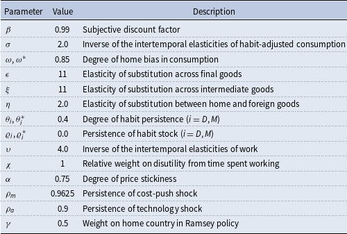
This section describes the parameters used in the simulations. Table 1 summarizes the parameter calibrations. We set the discount rate
 $\beta$
to 0.99. The relative risk aversion
 $\sigma$
(or the inverse of the habit-adjusted intertemporal substitution of consumption) is set to 2.0, while the elasticity of substitution between home and foreign goods
 $\eta$
is set to 2.0. Clarida et al. (Reference Clarida, Galí and Gertler2002) and Pappa (Reference Pappa2004) showed that a shock occurring in one country has a positive spillover effect on the other country when
 $\sigma \eta \gt 1$
in their models. This feature of the spillover effect carries over to our model.
Structural parameter values used in simulations

Following Ravn et al. (Reference Ravn, Schmitt-Grohe and Uribe2007), we assume that the degree of habits is equal among countries and goods.Footnote
19
Specifically, we set
 $\theta _D = \theta _M^* = \theta _M = \theta _D^* = \theta = 0.4$
. We use this value as a baseline; the following sections compare impulse responses in cases with and without a deep consumption habit. This value might be lower than that of previous studies. According to Leith et al. (Reference Leith, Moldovan and Rossi2012, Reference Leith, Moldovan and Rossi2015), macro-based estimates of deep habits vary from a relatively low value of 0.53, as in Ravn et al. (Reference Ravn, Schmitt-Grohé and Uribe2012), to extremely high values of 0.95–0.97, as in Ravn et al. (Reference Ravn, Schmitt-Grohé and Uribe2006) and Lubik and Teo (Reference Lubik and Teo2014). At the same time, micro-based estimates have much lower values of 0.29–0.5 (Ravina Reference Ravina2019).
Note that the determinacy problems should be considered as much as empirical plausibility. Models with deep habits are prone to indeterminacy due to the countercyclical markup behavior (Zubairy Reference Zubairy2014; Ravn et al. Reference Ravn, Schmitt-Grohe, Uribe and Uuskula2010; Jacob and Uusküla Reference Jacob and Uusküla2019).Footnote
20
The interaction caused by deep habits might be more reinforced in our two-country model with sticky prices, raising concerns about model stability. To avoid the problem, we keep the degree of habit somewhat lower. We use
 $ \theta = 0.4$
as a benchmark and compare the results to cases without deep habits (
 $ \theta = 0$
).
We set the degree of home bias
 $\omega$
to 0.85, following Bodenstein et al. (Reference Bodenstein, Guerrieri and LaBriola2019). For most of the remaining parameters, we followed Leith et al. (Reference Leith, Moldovan and Rossi2015, Reference Leith, Moldovan and Rossi2009). We set the elasticity of substitution for both final
 $\epsilon$
and intermediate goods
 $\xi$
to 11, the degree of price stickiness
 $\alpha$
to 0.75, and the Frisch labor supply elasticity (inverse of the intertemporal elasticity of work)
 $\upsilon$
to 4.0. Furthermore, we set the AR(1) coefficients for technology and cost-push shocks to
 $\rho _{a}=0.9$
and
 $\rho _{m}=0.9625$
, respectively. The relative weight of the disutility of labor
 $\chi$
is set to 1, We set the home country weight in the coordinated Ramsey policy to
 $(1-\gamma )=$
0.5.
5.2. Moments matching of the model with real economy data
This subsection analyzes the impact of incorporating deep habit formation on business cycle moments. As discussed in Sections 1 and 2, like superficial habits, deep habits generate a hump-shaped response of macroeconomic variables to economic shocks, as shown in Christiano et al. (Reference Christiano, Eichenbaum and Evans2005), Leith et al. (Reference Leith, Moldovan and Rossi2012) and Givens (Reference Givens2016). Moreover, replacing superficial habits with deep habits improves the fit between the impulse responses to monetary shocks and those estimated from structural VAR models, as reported by Ravn et al. (Reference Ravn, Schmitt-Grohe, Uribe and Uuskula2010) and Givens (Reference Givens2016). Additionally, deep habits induce a crowding-in effect of government spending, aligning with empirical evidence, as highlighted by Ravn et al. (Reference Ravn, Schmitt-Grohé and Uribe2006); Ravn et al. (Reference Ravn, Schmitt-Grohe, Uribe and Uuskula2010). In open economy models, Chari et al. (Reference Chari, Kehoe and McGrattan2002) emphasized the importance of incorporating consumption persistence to account for the persistence of real exchange rates; habit formation in consumption is a candidate for achieving this persistence.
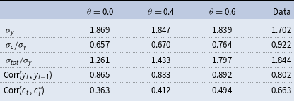
We evaluate its empirical fit to examine whether these characteristics are carried over in the two-country model presented in this study. Specifically, we follow Backus et al. (Reference Backus, Kehoe and Kydtand1995) and Ravn et al. (Reference Ravn, Schmitt-Grohe and Uribe2007) and use long-term available data from the United States (US) and Canada. We compute the relative standard deviations and correlation coefficients of output, consumption, and terms of trade, comparing the statistical moments from actual data with those generated by the model. Table 2 compares business cycle moments derived from the benchmark model with those observed in the data.
Empirical validation of a two-country sticky price model with deep habits: business cycle moments

Note:
 $\sigma _y$
denotes the standard deviation of output.
 $\sigma _c / \sigma _y$
and
 $\sigma _{tot} / \sigma _y$
represent the relative volatilities of consumption and terms of trade to output, respectively.
 $\text{Corr}(y_t, y_{t-1})$
captures the autocorrelation of output.
 $\text{Corr}(c_t, c_t^*)$
measures the correlation between domestic and foreign consumption.
 $\theta$
denotes the degree of deep habit. All data are from the Federal Reserve Economic Data (FRED) database of the Federal Reserve Bank of St. Louis. For the US, output is measured as per capita real GDP, seasonally adjusted annually, deflated by the consumer price index. Consumption is represented by per capita personal consumption expenditure, also seasonally adjusted at an annual rate. The terms of trade data are seasonally adjusted in a quarterly series. Due to data limitations, we use aggregate terms of trade rather than the bilateral terms of trade between the US and Canada. For Canada, GDP is measured as seasonally adjusted quarterly nominal GDP, deflated by the Canadian consumer price index to obtain real GDP. Consumption is represented by seasonally adjusted nominal household final consumption expenditure quarterly. We apply the Hodrick–Prescott (HP) filter to remove trends with a smoothing parameter of
 $\lambda = 1600$
. The sample period spans 200 quarters, from Q3 1973 to Q2 2023, and the model-generated data also cover 200 periods.
Table 2 compares business cycle moments obtained from the model under different degrees of deep habit formation
 $(\theta = 0.0, 0.4, 0.6)$
with empirical data. All data are from the Federal Reserve Economic Data database of the Federal Reserve Bank of St. Louis. For the US, output is measured as per capita real gross domestic product (GDP), which is seasonally adjusted annually and deflated by the consumer price index. Consumption is represented by per capita personal consumption expenditure, also seasonally adjusted at an annual rate. The terms of trade data are seasonally adjusted in a quarterly series. Due to data limitations, we use aggregate terms of trade rather than the bilateral terms of trade between the US and Canada. For Canada, GDP is measured as seasonally adjusted quarterly nominal GDP, deflated by the Canadian consumer price index to obtain real GDP. Consumption is represented by seasonally adjusted nominal household final consumption expenditure quarterly. We apply the Hodrick–Prescott (HP) filter to remove trends with a smoothing parameter of
 $\lambda = 1600$
. The sample period spans 200 quarters (from Q3 1973 to Q2 2023), and the model-generated data also cover 200 periods.
The key statistics include the standard deviation of output
 $\sigma _y$
, capturing the magnitude of business cycle fluctuations, as well as the relative volatility of consumption to output
 $\sigma _c / \sigma _y$
, and the relative volatility of terms of trade to output
 $\sigma _{tot} / \sigma _y$
. Additionally, the table reports the autocorrelation of output
 $\text{Corr}(y_t, y_{t-1})$
and measures the persistence of business cycles and the correlation between domestic and foreign consumption
 $\text{Corr}(c_t, c_t^*)$
, reflecting the degree of international consumption comovement.
The results indicate that the model’s standard deviation of output
 $\sigma _y$
decreases as
 $\theta$
increases, approaching the empirical value of 1.702, though it remains slightly higher. The model underestimates the relative volatility of consumption
 $\sigma _c / \sigma _y$
compared to the empirical value (0.922); however, this measure increases with
 $\theta$
, improving the match. Similarly, the relative volatility of terms of trade
 $\sigma _{tot} / \sigma _y$
increases with
 $\theta$
, bringing it closer to the empirical value of 1.844. Regarding the persistence of output fluctuations, the model consistently overestimates
 $\text{Corr}(y_t, y_{t-1})$
, as its values remain higher than the empirical benchmark of 0.802. The international consumption correlation
 $\text{Corr}(c_t, c_t^*)$
is lower in the model than in the data (0.663); however, increasing
 $\theta$
improves the fit.Footnote
21
While a higher degree of deep habit formation enhances the model’s alignment with the data in certain dimensions—particularly in trade volatility and consumption correlation—discrepancies remain in output volatility and persistence. The results suggest that the model with deep habit formation can somewhat replicate the empirical moments of business cycles.
5.3. Impulse responses
This section observes the impulse responses of the foreign and the home country in the case of exogenous shocks that occurred in the foreign country. As in other open models, foreign shocks lead to spillovers to the home country. The spillover effects are affected by parameters specific to open models (e.g., the degree of economic openness). Furthermore, the nature of economic dynamics also depends on the degree of deep habit.; hence, the optimal policy response also varies. In the following, we observe the responses to productivity and cost-push shocks.
5.3.1. Impulse responses of foreign productivity shock
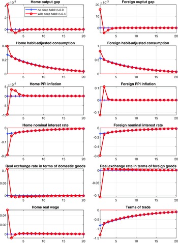
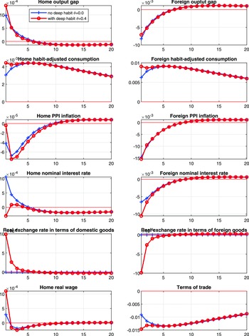
Figure 1 shows the impulse response to a productivity shock occurred in a foreign country. This figure compares impulse responses of the benchmark case (
 $\theta =0.4$
) with the case of no habit formation (
 $\theta =0$
).
Impulse responses to a foreign productivity shock: comparison with and without deep habit.

We first review the effects of foreign productivity shock on the foreign country. The effects of the shock align with the results of previous studies in a closed economy model—a positive productivity shock raises natural output and decreases pressure on inflation. Under optimal monetary policy, the central bank reduces these fluctuations by lowering interest rates. Thus, without deep habits, the central bank can fully control the fluctuations in inflation and the output gap associated with changes in productivity shocks. The solid blue line in Figure 1 (without deep habit) shows that the domestic inflation in a foreign country
 $\pi ^*_{D, t}$
and output gap
 $x_{t}^*$
are fully stabilized to the foreign productivity shocks.
In the case of deep habits, households tend to over-consume due to habit formation, leading to an increase in output deviating from the efficiency level (positive output gap). With deep habits, final goods firms are willing to lower the markups strategically to increase expected future demand, called the countercyclical response of markups or the intertemporal effect of deep habits (Ravn et al. Reference Ravn, Schmitt-Grohé and Uribe2006). In other words, final goods firms’ pricing behavior amplifies rather than stabilizes fluctuations in demand, which is consistent with the empirical evidence.Footnote 22
The above discussion is consistent with a closed economy case such as Leith et al. (Reference Leith, Moldovan and Rossi2015); however, the relationship between the degree of deep habits and the magnitude of decreases in nominal interest rate in an open economy model is quite different from that in closed and open economies. In a closed economy with deep habits, the central bank is reluctant to lower interest rates in response to productivity shock because lowering interest rates leads to decreased markups of final goods and increased household overconsumption. However, in an open economy model, the nominal interest rate is lower than without deep habit.
The key difference between closed and open economies is the role of terms of trade. In a closed economy with strong consumption habits, the central conflict arises from the need to stabilize domestic prices while internalizing habit-driven externalities. An additional challenge emerges in an open economy: internalizing the externalities of terms of trade. The central bank aims to limit interest rate cuts to mitigate habit externalities; however, it also faces incentives to lower rates to improve economic welfare through terms of trade effects.Footnote 23
As mentioned, deep habits generate the endogenous trade-off between stabilizing the output gap and inflation in a productivity shock that deviates from the “divine coincidence.”Footnote 24 Unlike the closed economy case, the greater the degree of habit formation, the stronger this effect will be.
Moreover, in an open economy model, the change in markups caused by productivity shocks and the resulting change in the demand function leads to different pricing at home and foreign destinations. This pricing strategy is based on the different demand curves, or LCP, and is the source of the deviation from the LOP. The deviation of LOP for foreign goods is equivalent to the good-specific real exchange rate for foreign goods
 $\psi _t^*$
.
With deep habit, the change in the terms of trade is greater, which leads to a more significant spillover effect on the home country. The intuition is as follows. Foreign productivity shocks increase foreign output, which worsens the terms of trade in a foreign country, with or without deep habits. Furthermore, with deep habits, the increase in foreign output causes habit formation and demand, which deviates from the LOP, causing the good-specific real exchange rate (Ravn et al. Reference Ravn, Schmitt-Grohé and Uribe2012). Due to the fluctuation of good-specific real exchange rates, the terms of trade deterioration is worse than in the open economy model without deep habit.
5.3.2. The role of degree of home bias in response to foreign productivity shock
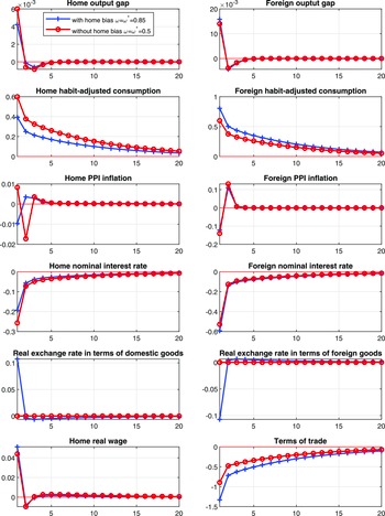
We next examine the impulse responses to productivity shocks with and without home bias in consumption while keeping the degree of deep habits at the baseline level of
 $\theta =0.4$
in Figure 2. This approach allows us to highlight the impacts specific to an open economy.
Impulse responses of a foreign productivity shock concerning changing the degree of home bias.

When transitioning from a baseline with home bias (
 $\omega = 0.85$
) to a case without home bias (
 $\omega = 0.5$
), increasing foreign production due to a foreign productivity shock results in a greater share of foreign goods being consumed in the home country as imported goods. This situation implies that the required adjustment in terms of trade for a given change in exports and imports is comparatively small. Consequently, the central bank’s incentive to manipulate the terms of trade weakens, leading to a more muted interest rate reduction than the case with home bias. As a result, fluctuations in the foreign country’s output gap, consumption, and inflation become smaller, improving economic welfare.
Interestingly, without home bias, i.e.,
 $\omega =0.5$
, the good-specific real exchange rate remains unchanged in response to productivity shocks. The absence of home bias in consumption implies that relative price changes between domestic and foreign goods in response to shocks are identical across countries, ensuring that LOP holds. Conversely, in the presence of home bias, a foreign productivity shock leads to a decline in the price of foreign goods abroad, while demand for and the price of foreign goods in the domestic market remain unchanged. This asymmetry in price responses to shocks generates deviations from the LOP and fluctuations in the good-specific real exchange rate. Hence, the greater the home bias, the larger the fluctuations in the good-specific real exchange rate and the terms of trade.Footnote
25
Without home bias, the spillover effect of foreign shocks on aggregate demand in the home economy intensifies. Thus, the domestic interest rate is more substantially lowered, causing greater volatility in consumption and the output gap in the home economy.
When deep habits exist, productivity shocks create a trade-off between output gap stabilization and inflation stabilization. Moreover, in open-economy models, markups of intermediate goods producers in both countries behave countercyclically, causing deviations from the LOP. These deviations imply that optimal interest rate responses in open economies with deep habits are more significant than in closed economies with deep habits. In contrast, without home bias, such deviations from the LOP do not arise, making the dynamics of an open economy with deep habits resemble a closed economy with deep habits.
5.3.3. Impulse responses of foreign cost-push shock
Figure 3 depicts the impulse responses to a reduction in the desired markup of foreign intermediate goods firms (1% increase in
 $\xi _t^*$
), or a negative foreign cost-push shock.
Impulse responses of a negative foreign cost-push shock: comparison with and without deep habit.

A decline in the desired markup incentivizes those adjusting prices to lower them toward the average, reducing inflation and increasing output; shock acts as a negative cost-push shock. Even without deep habits, the central bank faces a trade-off between inflation stability and the output gap.
As with a productivity shock, deep habits lead final goods producers to lower markups, prioritizing future demand over immediate profits. This results in pricing-to-market behavior, depreciating good-specific real exchange rates and worsening the terms of trade. In response to the negative foreign cost-push shock, the foreign central bank cuts interest rates more aggressively to counteract deflationary pressure; thus, the decline in foreign inflation remains similar to the case without deep habits.
This situation contrasts with closed-economy models, where deep habits prompt the central bank to raise interest rates temporarily to internalize consumption externalities, causing an initial markup increase before it declines. In a two-country model with deep habits, the central bank also considers terms of trade externalities; thus, this temporary markup increase does not occur.
Figure 4 illustrates this by reducing home bias from
 $\omega =0.85$
to
 $\omega =0.5$
. Similar to productivity shocks, the central bank exploits spillover effects through terms of trade adjustments. With lower home bias, the home country imports more foreign goods, allowing the central bank to reduce foreign markups further. Without home bias, firms no longer engage in pricing-to-market, muting good-specific real exchange rate movements; however, foreign shocks significantly impact the domestic economy.
Impulse responses of a negative foreign cost-push shock concerning changing the degree of home bias.

5.4. The role of policy coordination
This subsection calculates the gains from international policy coordination compared to the case of non-cooperative policies by home and foreign countries. Following Fujiwara and Wang (Reference Fujiwara and Wang2017), Kim (Reference Kim2023), the gain of coordination is given by
 \begin{align} E_t \beta ^j \sum _{j=0}^{\infty } \left [ (1-\gamma ) U_{1}((1+\Omega )X_{t+j}^{\text{nash}}, N_{t+j}^{\text{nash}}) + \gamma U_{2}(C_{t+j}^{*\text{nash}}, N_{t+j}^{*\text{nash}}) \right ] = (1-\gamma ) W_{1, t}^{\text{coop}} + \gamma W_{2, t}^{\text{coop}} \end{align}
where
 $W_{1, t}^{\text{coop}}$
and
 $W_{2, t}^{\text{coop}}$
are the cooperative welfare levels of the home and foreign country, respectively. Superscript “nash” and “coop” indicate non-cooperative open-loop Nash equilibrium and cooperative Ramsey equilibrium, respectively.
 $\Omega$
is the parameter of consumption-equivalent welfare loss, representing the unit of steady-state consumption that must be given up to achieve the same level of welfare as the Nash equilibrium in international cooperation. Appendix D provides the derivation of the solution to this equation concerning
 $\Omega$
.
5.4.1. Welfare gains of policy coordination in the case of symmetric home bias
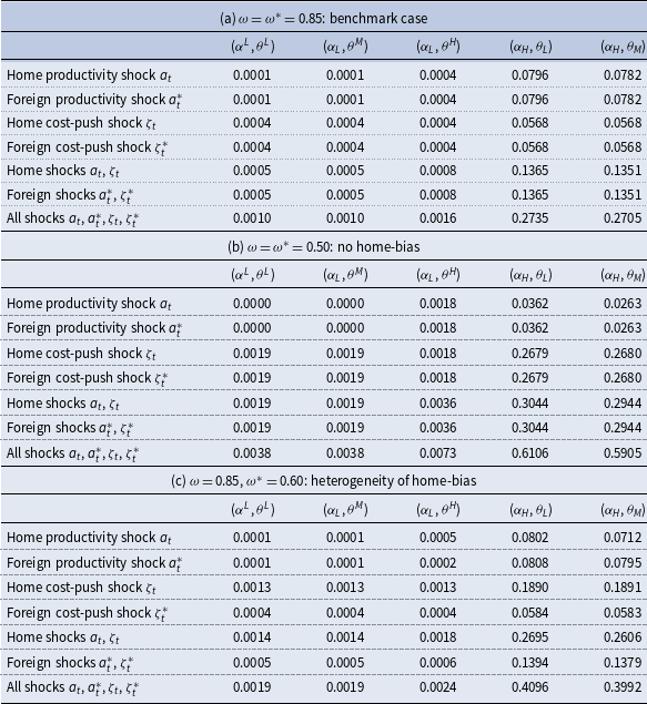
Table 3 shows welfare gains of policy coordination. The table divides the cases by the degree of stickiness price
 $\alpha$
and the degree of deep habits
 $\theta$
. Each row shows the exogenous economic shocks: home and foreign productivity, cost-push, and compound shocks. Each column shows a pair of price stickiness and the degree of deep habits.
 $\alpha ^L = 0.01$
(flexible price),
 $\alpha ^H = 0.75$
(sticky price),
 $\theta ^L = 0.0$
(no deep habit),
 $\theta ^M=0.1$
and
 $\theta ^H = 0.60$
. As mentioned, including deep habits in the model when prices are sticky can lead to instability, especially with non-cooperative policies. For example, when price rigidity is 0.75, the degree of deep habits yielding a stable Nash equilibrium solution is
 $\theta = 0.1$
at most. In contrast,
 $\theta$
can be a relatively large value when prices are flexible.
Welfare gains from policy coordination in a two-country model with sticky prices and deep habits

Note:
 $ \alpha ^L=0.01, \ \alpha ^H=0.75, \ \theta ^L=0.00, \ \theta ^M=0.10, \ \theta ^H=0.60$
and
 $\theta _D=\theta _D^*=\theta _M=\theta _M^*=\theta ^i$
for
 $i \in \{L, M, H\}$
.
Panel (a) in Table 3 is a benchmark case where home and foreign countries share the same value of home bias,
 $\omega =\omega ^*=0.85$
. Panel (a) shows when the price is flexible (in the case of
 $\alpha ^L$
). When the home bias is symmetric, the gains from international cooperation are equal regardless of whether the shock originates from a home or foreign country since all other conditions are symmetric. The gain is smaller than when prices are sticky
 $\alpha ^H$
, regardless of the type of shock or the presence of deep habits. This situation is unsurprising since price rigidity is one of the primary sources of market distortions. Flexible prices require little relative price adjustment, and even non-cooperation can yield desirable results; however, even when prices are flexible, the gain slightly increases as the degree of deep habits
 $\theta$
goes from 0.0 to 0.6.
When prices are sticky, the change in gains and their differences are marginal;
 $\theta$
can be from 0 to 0.1 at most due to the stability problems discussed above (especially in the non-cooperative case). However, when a deep habit exists, the gain decreases from 0.0796% to 0.0782% when the productivity shock is the source of fluctuation. In contrast, the effect of the degree of deep habits on the gains is negligible in the case of cost-push shocks.
The existence of deep habits with sticky prices reduces gains, indicating that reducing excessive consumption due to habits may benefit foreign countries. Habit consumption includes imported consumption, and reducing imported consumption will suppress foreign overproduction and over-labor. As a result, international desirability is almost achieved in non-cooperative policies, and the gain is smaller, particularly for productivity shocks. This result is also related to the degree of home bias. When the home bias is 0.85, the change is small, ranging from 0.0796% to 0.0782%. Conversely, in the case without home bias, panel (b), the change is relatively large, ranging from 0.0362% to 0.0263%. This result occurs because the effect of import inhibition is larger when there is no home bias.
5.4.2. Welfare gains of policy coordination in the case of no home bias
Panel (b) in Table 3 shows the case without home bias (
 $\omega =\omega ^*=0.50$
). Compared to the case with high home bias panel (a), a substantial difference occurs; however, the gain in the case of cost-push shocks is larger with or without deep habit. The existing discussion of international coordination can explain the difference in gains due to different degrees of home bias. In the case of productivity shocks, no trade-off occurs between inflation and the output gap (in the absence of deep habit); in contrast,cost-push shocks generate a policy trade-off. This trade-off gives countries more incentives to strategically manipulate their terms of trade to improve their economies; thus, there is more room for policy coordination to remove the distortion.
5.4.3. Welfare gains of policy coordination in the case of asymmetric home bias
Panel (c) in Table 3 shows the case of heterogeneous home bias. When the home bias differs between countries, the shock has policy implications regardless of the source. The difference in the origin of the shocks has no significant impact when prices are flexible or during productivity shocks; however, the difference is particularly pronounced in the case of cost-push shocks. For example, when
 $\omega =0.85, \omega ^*=0.60, \alpha =0.75$
, and
 $\theta =0.10$
, the gain with a cost-push shock in the home country is 0.1891; the gain in the case of foreign cost-push shock is 0.0583. Panel (b) shows that when a cost-push shock occurs in the home country, the home central bank attempts to increase its welfare through relative price adjustment by manipulating the terms of trade. In this case, it is relatively easy to cause expenditure switching as long as the home bias of the foreign country is smallFootnote
26
This distortion creates room for gains through policy coordination. Conversely, when a cost-push occurs in the foreign country, and the home bias is significant in the home country, households in the home country are unwilling to import foreign goods; thus, an expenditure switch in favor of the foreign country cannot occur.
These results remain unchanged regardless of the presence or degree of deep habits. Strong deep habits can have a significant influence; however, our calibrations do not indicate that their presence is sufficient to override the effects of terms of trade manipulation or price stabilization. Nonetheless, the deep habits may reduce the gains from policy coordination when specific conditions are met, such as productivity shocks, price rigidity, and the absence of home bias.
5.4.4. Impulse responses: Ramsey optimal policy and non-cooperative policy
Figure 5 compared impulse responses to a foreign productivity shock under international coordination (Ramsey) and non-coordination (Nash). In a two-country model with price stickiness and deep habits, equilibrium stability is particularly problematic in the Nash case; therefore, Figures 5 and 6 assume
 $\theta =0.1$
.
Impulse responses to a foreign productivity shock: cooperative Ramsey vs. non-cooperative open-loop Nash equilibrium.

Table 3 shows that the difference between coordinated and non-coordinated responses to productivity shocks is small. In contrast, Figure 5 indicates that the Ramsey policy results in a slightly larger interest rate cut than the Nash case. This situation reduces output gap and inflation volatility domestically, at the cost of slightly higher volatility in the foreign economy. In the Nash case, an incentive arises to manipulate terms of trade in favor of the foreign economy, whereas coordination internalizes this externality. Due to international policy coordination, the spillover of productivity shocks from foreign economies to the domestic economy is more limited than the Nash equilibrium, leading to a smaller reduction in domestic interest rates under coordination. The interest rate cut stimulates greater demand and production in the noncooperative case, causing an increase in real wages, a larger output gap, and higher inflation in the domestic economy. This difference in the sign of domestic inflation rates between coordinated and noncoordinated outcomes reflects these dynamics.
Figure 6 examines impulse responses to a negative foreign cost-push shock under coordination and non-coordination, yielding similar insights. Coordination slightly increases the foreign output gap and inflation volatility while stabilizing the domestic output gap; thus, the foundation of international coordination is the monetary policy that internalizes both terms of trade and consumption externalities from deep habits.
Impulse responses of a negative foreign cost-push shock: cooperative Ramsey vs. non-cooperative open-loop Nash equilibrium.

The differences in interest rate adjustments between the domestic and foreign economies primarily drive the gains from policy coordination. In the noncooperative case, foreign interest rates are adjusted more aggressively to counter shocks abroad, while in the coordinated case, these changes are more restrained. This situation also results in a more moderate change in domestic interest rates. Consequently, foreign volatility is slightly higher under coordination, while domestic volatility is somewhat lower compared to the non-cooperative outcome. These results reflect the spillover effects of terms of trade adjustments, incorporating the distortions in demand caused by habit formation.
6. Concluding remarks
Our paper shows how the dependence between the deep habits in consumption and optimal monetary policy in the closed NK model may differ when extended to a two-country NK model. We calibrate the model parameters and assess the model’s fit to real-world data by comparing moments, focusing on the empirical validity of deep habits. Our findings indicate that incorporating deep habit formation improves the model’s fit to empirical data, particularly regarding trade volatility and consumption correlation, suggesting that the model reasonably approximates business cycle dynamics.
Furthermore, in response to the structural shocks, the central bank changes the interest rate aggressively in the two-country open economy model. This result contrasts with a closed economy, where the central bank is reluctant to move interest rates. When there is a deep habit in consumption, the international central bank can exploit the externalities of the terms of trade. Habit formation might boost the expenditure-switching effect, which differentiates the aggressiveness of the central bank between closed and open economies with deep habits. This result occurs because habitual consumption does not generate utility, meaning that intratemporal substitution from aggregate consumption to leisure via exploiting terms of trade may improve welfare efficiently by reducing meaningless habitual consumption.
Furthermore, the deviations from the LOP, or the good-specific real exchange rate, generated by the deep habits are related to the degree of home bias. In particular, the deviations fully disappear with no home bias.
Moreover, our results suggest that international monetary policy coordination offers welfare gains, especially when prices are sticky; however, coordination is less beneficial when deep habits are present, particularly in response to productivity shocks. The degree of home bias is also influential, with higher home bias leading to more uniform coordination benefits across shocks. Furthermore, policy coordination can address inefficiencies from price stickiness and consumption habits; however, it is not always indispensable. Deep habits may reduce coordination gains under certain conditions, and non-cooperative outcomes can remain relatively efficient, especially with flexible prices.
Our study considered an optimally coordinated central bank; however, the discretionary policy was not considered. Therefore, investigating the gain in commitment, as in Givens (Reference Givens2016), is one possible avenue for future research.
Acknowledgements
The author thanks William A. Barnet (Editor) and two anonymous referees for their valuable feedback and insightful suggestions, as well as Daisuke Ida for helpful comments and suggestions. All remaining errors are the author’s.
Funding statement
This paper was supported by JSPS KAKENHI (grant nos. 20K13531 and 20K01784).
Supplementary material
The supplementary material for this article can be found at https://doi.org/10.1017/S1365100525100187.