


Malnutrition is a major global public health problem affecting more than one billion of the world’s population(Reference Cederholm, Barazzoni and Austin1,Reference Wang, Barazzoni and Shi2) . It is also a highly prevalent disorder in oncology practice(Reference Arends, Bachmann and Baracos3–Reference Yin, Lin and Liu5) with a prevalence of 21 % to 72 %(Reference Gioulbasanis, Baracos and Giannousi6–Reference Hu, Barazzoni and Shi8). Malnutrition can impede the efficacy and safety of anticancer therapies(Reference Arends, Bachmann and Baracos3), increase healthcare resource utilisation(Reference Yin, Song and Cui4) and lead to multiple adverse outcomes(Reference Rosato, Gigante and Colalillo9,Reference Brown, Loeliger and Stewart10) . In fact, an estimated 10–20 % of cancer deaths are solely ascribable to malnutrition(Reference Arends, Baracos and Bertz11). However, due to a lack of proper diagnostic techniques and sufficient attention, cancer-associated malnutrition remains largely underreported(Reference Gyan, Raynard and Durand12), misclassified(Reference Attar, Malka and Sabate13) or left untreated(Reference Hebuterne, Lemarie and Michallet14). Therefore, active diagnosis, surveillance and intervention of malnutrition are imperative in all cancer patients to minimise or reverse its negative impact on patient outcomes(Reference Arends, Bachmann and Baracos3,Reference Yin, Song and Cui4,Reference Arends, Baracos and Bertz11,Reference Kipouros, Vamvakari and Kalafati15) .
The practical criteria used to diagnose malnutrition vary across different institutions(Reference Gioulbasanis, Baracos and Giannousi6,Reference Gyan, Raynard and Durand12–Reference Hebuterne, Lemarie and Michallet14) , making it difficult to implement a universally standardised framework for patient management. To address this challenge, an international consensus-based conceptual framework was proposed in 2019(Reference Cederholm, Jensen and Correia16), the Global Leadership Initiative on Malnutrition (GLIM), for diagnosing malnutrition in adults in clinical settings. Briefly, for patients who are screened positive for nutritional risk, at least one phenotypic criterion and one aetiological criterion are required to diagnose malnutrition(Reference Cederholm, Jensen and Correia16). This new framework effectively incorporates the evolving understanding and current evidence on malnutrition, making it a promising tool with global acceptance potential(Reference Yin, Lin and Liu5,Reference Brown, Loeliger and Stewart10,Reference Murnane, Forsyth and Koukounaras17–Reference Yin, Lin and Li21) .
Since its release, the GLIM framework has proven to be valuable in diagnosing malnutrition and predicting clinical outcomes across a wide range of diseases(Reference Rosato, Gigante and Colalillo9,Reference Brown, Loeliger and Stewart10,Reference Milanez, Razzera and Lima22) . In the context of cancer, evidence from our research(Reference Yin, Chong and Huo20,Reference Yin, Lin and Li21,Reference Yin, Fan and Lin23,Reference Yin, Cheng and Chen24) and other institutions(Reference Brown, Loeliger and Stewart10,Reference Murnane, Forsyth and Koukounaras17–Reference Kiss, Steer and de van der Schueren19,Reference Peng, Zong and Yang25,Reference Liu, Lu and Li26) consistently demonstrates that GLIM-defined malnutrition is associated with worse clinical outcomes, including postoperative complications(Reference Brown, Loeliger and Stewart10,Reference Murnane, Forsyth and Koukounaras17,Reference Matsui, Rifu and Watanabe18,Reference Peng, Zong and Yang25,Reference Liu, Lu and Li26) , length of hospital stay(Reference Yin, Fan and Lin23,Reference Liu, Lu and Li26) , in-hospital mortality(Reference Liu, Lu and Li26), thirty-day mortality(Reference Kiss, Steer and de van der Schueren19), disease-free survival(Reference Matsui, Rifu and Watanabe18,Reference Peng, Zong and Yang25) and/or overall survival(Reference Kiss, Steer and de van der Schueren19–Reference Yin, Lin and Li21,Reference Yin, Fan and Lin23,Reference Yin, Cheng and Chen24) . Moreover, the GLIM framework has been found to outperform the International Classification of Diseases 10th Revision criteria in identifying more malnourished patients and establishing a stronger correlation with surgical risk(Reference Murnane, Forsyth and Koukounaras17). These findings underscore the superiority and clinical relevance of the GLIM framework in patients with cancer(Reference Yin, Cheng and Chen24). However, it is important to note that existing studies have focused on the presence of malnutrition at a single time point, mainly at baseline(Reference Rosato, Gigante and Colalillo9,Reference Brown, Loeliger and Stewart10,Reference Murnane, Forsyth and Koukounaras17,Reference Matsui, Rifu and Watanabe18,Reference Yin, Chong and Huo20,Reference Milanez, Razzera and Lima22,Reference Yin, Cheng and Chen24,Reference Liu, Lu and Li26,Reference Barazzoni, Jensen and Correia27) . To our knowledge, no study has investigated the transition of GLIM-defined malnutrition within a clinically operational timeframe in cancer. Considering the variability in responses to malnutrition and its treatment among individuals(Reference Arends, Bachmann and Baracos3,Reference Arends, Baracos and Bertz11) , an approach that can identify patients who may benefit from multidisciplinary treatment and/or are likely to recover from malnutrition would be valuable for making individualised management decisions.
Weight loss, BMI and muscle mass are key elements used to identify, phenotype and grade malnutrition(Reference Cederholm, Jensen and Correia16). Additionally, these factors are useful in predicting future risks of weight loss(Reference O’Donoghue, Shrotriya and Aktas28) and muscle loss(Reference Hsu, Ko and Weng29). However, no studies have yet used weight and muscle information to predict the future outcomes of malnutrition. Based on this understanding, we hypothesise that body weight and muscle dynamic data routinely accessible upon patient admission can independently predict the fate of malnutrition. In this study, we proposed a deep learning model for early identification of reversible malnutrition (RM) in patients with cancer. The primary objective of this study was to enhance the decision-making of cancer-associated malnutrition to optimise patient outcomes.
Materials and methods
Study design and population
This was a retrospective cohort study conducted at multiple centres in China with prospectively collected data. Patients were derived from the Investigation on Nutrition Status and its Clinical Outcome of Common Cancers which was registered online (http://www.chictr.org.cn/showproj.aspx?proj=31813, identifier: ChiCTR1800020329). The Investigation on Nutrition Status and its Clinical Outcome of Common Cancers is a clinical research project initiated by the Chinese Society for Nutritional Oncology since 2013. The aim of Investigation on Nutrition Status and its Clinical Outcome of Common Cancers is to determine the prevalence of malnutrition in inpatients with cancer in China and to examine its relationship with the clinical outcomes. The project protocol has been published previously,(Reference Xu, Song and Yin30) and the inclusion and exclusion criteria for participants are detailed in online Supplementary Table S1. In accordance with these criteria, we initially included 30 766 patients aged over 18 years who were first diagnosed with cancer and/or were hospitalised for anti-cancer treatment from December 2013 to May 2021. Further exclusions were made for patients who lacked required body weight dynamic data (n 16 054), had outlier values (n 71), had unclear pathological results (n 567) and did not meet the baseline malnutrition criteria according to the GLIM framework (n 9832)(Reference Cederholm, Jensen and Correia16). This left 4254 patients with diagnosed malnutrition for formal analysis. A flowchart illustrating the patient inclusion process is presented in online Supplementary Figure S1. A cohort including 798 malnourished oncology patients (the Yunnan cohort), which was independent of the study population, was used for further model validation. The study was approved by the Ethics Committee of Army Medical Center of PLA (approval number: 2018-22), and written consent was provided by all patients. All data were de-identified before analysis, and the principles of the Declaration of Helsinki were followed. The Strengthening and Reporting of Observational Studies in Epidemiology Statement was followed.
Data acquisition and handling
Data were collected through in-person interview and physical examination by project-trained researchers within the first 48 h after patient admission: patient age, sex, smoking status (active tobacco smoker in the past one year), alcohol drinking (once a week or more frequent alcohol consumption in the past one year, regardless of amount and type), tea drinking (once a week or more frequent tea consumption in the past one year, regardless of amount and type), residency (urban v. rural), occupation (blue v. white collar), body height, body weight (six months before, one month before, at the time of, and one month after baseline, these time points were abbreviated as −6, −1, baseline and +1), BMI, weight loss, mid-arm circumference, triceps skinfold thickness, handgrip strength, mid-arm muscle circumference, calf circumference, appendicular skeletal muscle mass index (ASMI), food intake, gastrointestinal symptoms, the Eastern Cooperative Oncology Group physical performance score, the Nutritional Risk Screening 2002 score(Reference Kondrup, Allison and Elia31), the Patient-Generated Subjective Global Assessment (PG-SGA) score(Reference Ottery32) and the quality of life score (using the global quality of life score of the European Organization for Research and Treatment of Cancer QLQ-C30 scale).
The detailed approaches used, including the formulas, procedures and devices used to obtain the anthropometric indices (height, weight, BMI, weight loss, mid-arm circumference, triceps skinfold thickness, handgrip strength, mid-arm muscle circumference, calf circumference and ASMI), are shown in online Supplementary Table S2. The BMI (kg/m2) was as also categorised as underweight (< 18·5), normal (18·5 to < 24), overweight (24 to < 28) or obese (≥ 28) according to the Chinese recommendations(Reference Chen and Lu33). The gastrointestinal symptoms of patients were assessed in accordance with the PG-SGA(Reference Ottery32). Cancer cachexia was retrospectively diagnosed and staged using the Fearon’s framework(Reference Fearon, Strasser and Anker34). The clinical characteristics recorded during hospitalisation, including the comorbidities, cancer site, clinical tumor stage, anticancer therapies received, nutritional support received, laboratory indices, the Eastern Cooperative Oncology Group score one month after admission was retrospectively retrieved from electronic medical records. Body weight one month after admission was either measured (if hospital stay ≥ 30 d), or patient-reported via a follow-up after discharge (if hospital stay < 30 d).
Definitions of malnutrition and reversible malnutrition
Malnutrition was retrospectively diagnosed based on the GLIM criteria(Reference Cederholm, Jensen and Correia16). Briefly, for patients who were at nutritional risk (Nutritional Risk Screening 2002 ≥ 3), at least one phenotypic criterion and one aetiologic criterion needed to be met to diagnose malnutrition. The phenotypic criteria were involuntary weight loss 5–10 % within the past 6 months, or 10–20 % beyond 6 months; BMI < 18·5 kg/m2 if <70 years, <20 kg/m2 if ≥70 years(Reference Yin, Song and Cui4) or reduced muscle mass (ASMI, male < 7·0 kg/m2 or female < 5·4 kg/m2, based on the Asian Working Group for Sarcopenia 2019 Consensus(Reference Chen, Woo and Assantachai35)). For the aetiologic criteria, the entire study population was considered positive for the disease burden-related etiologic criterion since all patients were pathologically diagnosed with cancer and/or hospitalised for cancer treatment(Reference Yin, Song and Cui4). The diagnosis of malnutrition was independently performed at baseline and one month after baseline. RM was the primary outcome of the study, defined as a diagnosis of malnutrition at baseline (upon patient admission) turning negative one month later (all three phenotypic criteria being negative).
Machine learning models building
The study population (n 4254) was shuffled and randomly split into a discovery set (n 2977, 70 %) for model training and a holdout test set (n 1277, 30 %) to evaluate the model performance. The Yunnan cohort (n 798) was used as an external validation set (online Supplementary Figure S2). Based on the study hypothesis, feature selection was performed by manually selecting variables related to body weight and muscle dynamics that can be obtained upon patient admission. This approach was found to be feasible in our previous research(Reference Yin, Li and Lin36,Reference Yin, Zhang and Li37) . Six variables, including BMI and ASMI at −6, −1 and baseline, were defined as input variables, and RM (yes v. no) was defined as the binary outcome variable. The input data were standardised using a Z-score approach before modeling (Equation 1, where x represents raw score, μ represents mean, σ represents standard deviation).
 $$Z = \;{{x - \mu }\over{\sigma }}$$
Since the input variables are time-series data, we used a long short-term memory recurrent neural network architecture for modelling to capture the sequential information. The model was named as WAL-net (representing weight, appendicular skeletal muscle and long short-term memory-based deep neural network). The WAL-net was trained using a 32-sample mini-batch technique with a binary cross-entropy loss function (Equation 2, where N represents the total number of mini-batch samples, i represents an index that iterates over each sample from 1 to N, y i represents the true label of the i-th sample, p represents probability) and an Adam optimiser at a learning rate of 0·001.
 $$Loss = -{1 \over N} \mathop \sum \limits ^N_{i=1} {y_i} \cdot {log (p({y_i})) + (1 - {y_i})} \cdot {log (1 - p({y_i}))}$$
A detailed architecture of the WAL-net is shown in online Supplementary Figure S3. Accuracy, AUC, recall, precision, F1 score, Kappa and Matthews correlation coefficient were used as model comparison metrics, with higher values indicating better prediction performance(Reference Yin, Liu and Liu38). We also utilised sensitivity, specificity, positive predictive value and negative predictive value to evaluate and demonstrate the performance of the model, as these metrics are more commonly used in clinical scenarios(Reference Yin, Song and Cui4,Reference Yin, Lin and Liu5,Reference Yin, Cui and Lin39) . To verify the superiority of the WAL-net, another 19 conventional machine learning (ML) algorithms were independently developed for the same binary classification task. A ten-fold cross-validation with ten iterations technique (online Supplementary Figure S4) was used to aggregate model performance metrics for comparison and to select model with optimal hyper-parameters. The optimal model among the nineteen ML algorithms was then compared with the WAL-net in the holdout test set. The WAL-net was also assessed in different subgroups of the test set, including age, sex, cancer site, clinical stage, curative surgery, curative chemotherapy, nutritional support, C-reactive protein, the Eastern Cooperative Oncology Group score and PG-SGA score to evaluate potential effect modifications. The explainability of the model was evaluated using a shapley additive explanations (SHAP) method at both the group and individual levels. A decision curve analysis was used to evaluate the model’s clinical usefulness. Finally, the WAL-net was deployed as a prototypic web-based application for online prediction. The project code and files have been stored online in our GitHub repository (https://github.com/kevinlyy/rmalnutrition) for public access.
Statistical analysis
Continuous data were expressed as the medians (interquartile range) and compared using a Wilcoxon’s rank-sum test. Continuous data with multiple groups were compared using a pairwise Wilcoxon’s rank-sum test, and P values of multiple comparisons were adjusted using a Bonferroni’s method. Categorical data were expressed as numbers (percentage) and were compared using a χ 2 test. Cut-off values of the input variables to predict RM were calculated by maximising the Youden’s index (sensitivity + specificity − 1) in the discovery set. The generated cut-offs were then assessed in the holdout test set. Model-predicted probability greater than 0·5 was defined as the cut-off point for belonging to the RM group. All reported P values were two-sided and considered significant at P < 0·05. All analyses were performed using R (version 4.3.1, Foundation for Statistical Computing, Vienna, Austria). Deep learning and other ML algorithms were conducted in Python (version 3.9.11, The Python Software Foundation, USA).
Results
Population overview
The baseline characteristics of the study population are shown in the overall column of Table 1. There were 4254 patients with a median age of 61 years, including 2783 males and 1471 females. The tumours were most frequently located in the lung (n 984, 23·1 %), colorectum (n 870, 20·5 %), stomach (n 749, 17·6 %), oesophagus (n 416, 9·8 %) and nasopharynx (n 267, 6·3 %). The number of cases for all cancer sites is shown in Figure 1(a). The predominant clinical tumour stages were II (32·4 %) and III (31·2 %).
General characteristics of the study population

EN, enteral nutrition support; PN, parenteral nutrition support; ALT, alanine transaminase; AST, alkaline phosphatase; HDL, high-density lipoprotein; LDL low-density lipoprotein; NLR, neutrophil:lymphocyte ratio; MAC, mid-arm circumference; TSF, triceps skinfold thickness; MAMC, mid-arm muscle circumference; −six, six months before admission; −one, one month before admission; +one, one month after admission; ASMI, appendicular skeletal muscle mass index; GI, gastrointestinal; ECOG, the Eastern Cooperative Oncology Group; PG-SGA, the patient generated subjective global assessment; QoL, quality of life.
* Median (interquartile range), all such values, compared using Wilcoxon’s rank-sum test.
† Number (percentage), all such values, compared using a χ 2 test.
‡ Haematological malignancies are not included for clinical staging.
§ Assessed using the European Organization for Research and Treatment of Cancer QLQ-C30 scale (QLQ-C30). The global QoL scale in QLQ-C30 was used with a higher score indicating a better global QoL.
Prevalence of reversible malnutrition and analysis on the dynamics of body weight and muscle. IQR, interquartile range; RM, reversible malnutrition; −Six (t1), six months before baseline; −One (t2), one month before baseline; baseline (t3), upon patient admission; +One (t4), one month after baseline; ASMI, appendicular skeletal muscle mass index; ***, P < 0·001. (a) Number of cases for each cancer site. (b) Cancer-specific prevalence of reversible malnutrition. (c) BMI dynamics across the four time points. (d) BMI dynamics across the four time points stratified by the RM status. (e) Appendicular skeletal muscle index dynamics across the four time points. (f) Appendicular skeletal muscle index dynamics across the four time points stratified by the RM status.

Reversible malnutrition
RM was found in 754 (17·7 %) patients, while the remaining patients exhibited at least one positive phenotypic criterion one month following baseline. The prevalence of RM was further analysed based on the specific cancer sites as shown in Figure 1(b). The RM was most frequently observed in prostate cancer (34·8 %), brain cancer (25·0 %) and multiple myeloma (25·0 %), while being least prevalent in cancers located in the biliary tract (5·3 %), ovary (5·4 %) and oesophagus (8·4 %).
Dynamics of body weight and skeletal muscle
The BMI and ASMI dynamics over the four time points (−6, −1, baseline and +1) were assessed (Figure 1(c)–(f) and Table 1). Across the four time points, there was a significant downward trend in BMI within the study population (Figure 1(c)). In stratified analysis, RM and non-RM groups showed significant difference in the patterns of BMI changes (Figure 1(d)). Briefly, the RM group has higher BMI than the non-RM group at the −6, −1 and +1 time points, but lower BMI at baseline. In-group multiple comparison showed that the BMI change was significant in all time intervals except for the −6 v. −1 (P = 0·060), −6 v. +1 (P = 0·740) and −1 v. +1 (P = 0·430) intervals for the RM group. In contrast, the BMI change was significant in all time intervals except for the −1 to 0 interval for the non-RM group. Regarding ASMI, there was a significant downward trend within the study population across the whole pre-admission interval (−6 to 0) but not the 0 to +1 interval (P = 0·930, Figure 1(e)). In stratified analysis (Figure 1(f)), the RM group has higher ASMI than the non-RM group at all four time points. In-group multiple comparison showed that the ASMI was significantly increased in the 0 to +1 interval (P = 0·049) for the RM group. In contrast, the ASMI change was only insignificant in the 0 to +1 interval (P = 0·220) for the non-RM group. Heatmaps for the distribution of BMI and ASMI at different time points stratified by cancer site in the overall, RM and non-RM groups are shown in online Supplementary Figure S5. The results were similar to the findings observed in the overall population, indicating distinct patterns of BMI and ASMI dynamics between the RM and non-RM groups.
Reversible malnutrition and patient characteristics
The baseline characteristics of the study population, as stratified by the RM status, are shown in Table 1. RM was significantly associated with higher values/rates of male sex, smoking, tea drinking, diabetes, curative chemotherapy, total protein, creatinine, albumin, urea nitrogen, prealbumin, glucose, TAG, alkaline phosphatase, Hb, lymphocytes, erythrocytes, body height, mid-arm circumference, triceps skinfold thickness, handgrip strength, mid-arm muscle circumference, calf circumference, normal physical performance and global quality of life score. In contrast, RM was associated with lower values/rates of age, blue collar occupation, curative radiotherapy, nutritional support, platelets, C-reactive protein, neutrophil to lymphocyte ratio, anorexia, nausea, vomiting, constipation, dry mouth, taste changes, smell changes, dysphagia, early satiety and the PG-SGA score. In addition, the cancer sites, nutritional support type, food intake and the the Eastern Cooperative Oncology Group score category were also different between the RM and non-RM groups (all P < 0·05).
Reversible malnutrition and stages of cancer cachexia
The association between RM and stages of cancer cachexia was analysed in the overall population and in subgroups of cancer site (Figure 2 and online Supplementary Table S3). Compared with the non-RM group, the RM group was associated higher non-cachexia (41·5 % v. 9·8 %) and pre-cachexia rates (4·6 % v. 2·4 %) rates, but with lower cachexia (cachexia = 53·8 % v. 87·1 %) and refractory cachexia (0 % v. 0·7 %, P < 0·001) rates. Notably, all patients with refractory cachexia were classified into the non-RM group. Moreover, a spearman’s rank correlation analysis revealed a negative relationship between the progressive stages of cancer cachexia and RM (r = −0·340, P < 0·001). Subgroup analysis in gastrointestinal, respiratory, haematologic and others cancers revealed similar results (all P < 0·001).
Association between reversible malnutrition and stages of cancer cachexia in the overall population and in subgroups of cancer sites. RM, reversible cachexia; ***, P < 0·001.

Model training, comparison and assessment
A graphical workflow of the WAL-net is shown in Figure 3(a). The WAL-net starts with a long short-term memory layer to extract latent information from the sequential data of BMI and ASMI at three time points. After data processing with two fully-connected layers separated by a rectified linear unit (ReLU) layer, the model outputs a probability vector of the two outcome labels, which is subsequently normalised using the softmax function.
WAL-net and analyses on its superiority. ASMI, appendicular skeletal muscle index; LSTM, long short-term memory; WAL, weight, appendicular skeletal muscle and LSTM; MLP, multilayer perceptron; SVM, supportive vector machine; MCC, Matthews correlation coefficient; ROC, receiver operating characteristic. (a) A graphical workflow of the WAL-net. (b) Cross-validated results of machine learning models to predict reversible malnutrition in the discovery data. (c) ROC curves for the MLP model in the test data. (d) ROC curves for the WAL-net in the test data.

Distributions of the study variables in the discovery and test sets are shown in Table 1. We first trained the 19 ML models by setting the six variables of BMI and ASMI as the input variables and the RM (yes v. no) as the outcome variable in the discovery set. The ten-fold cross-validated results of the 19 ML models are shown in Figure 3(b). The multi-layer perceptron (MLP) model showed the highest performance, with an accuracy = 0·899, AUC = 0·839, recall = 0·536, precision = 0·831, F1 score = 0·647, Kappa = 0·591 and Matthews correlation coefficient = 0·613. Therefore, the MLP model was selected among the nineteen conventional ML models for future use, with its hyper-parameters shown in online Supplementary Table S4.
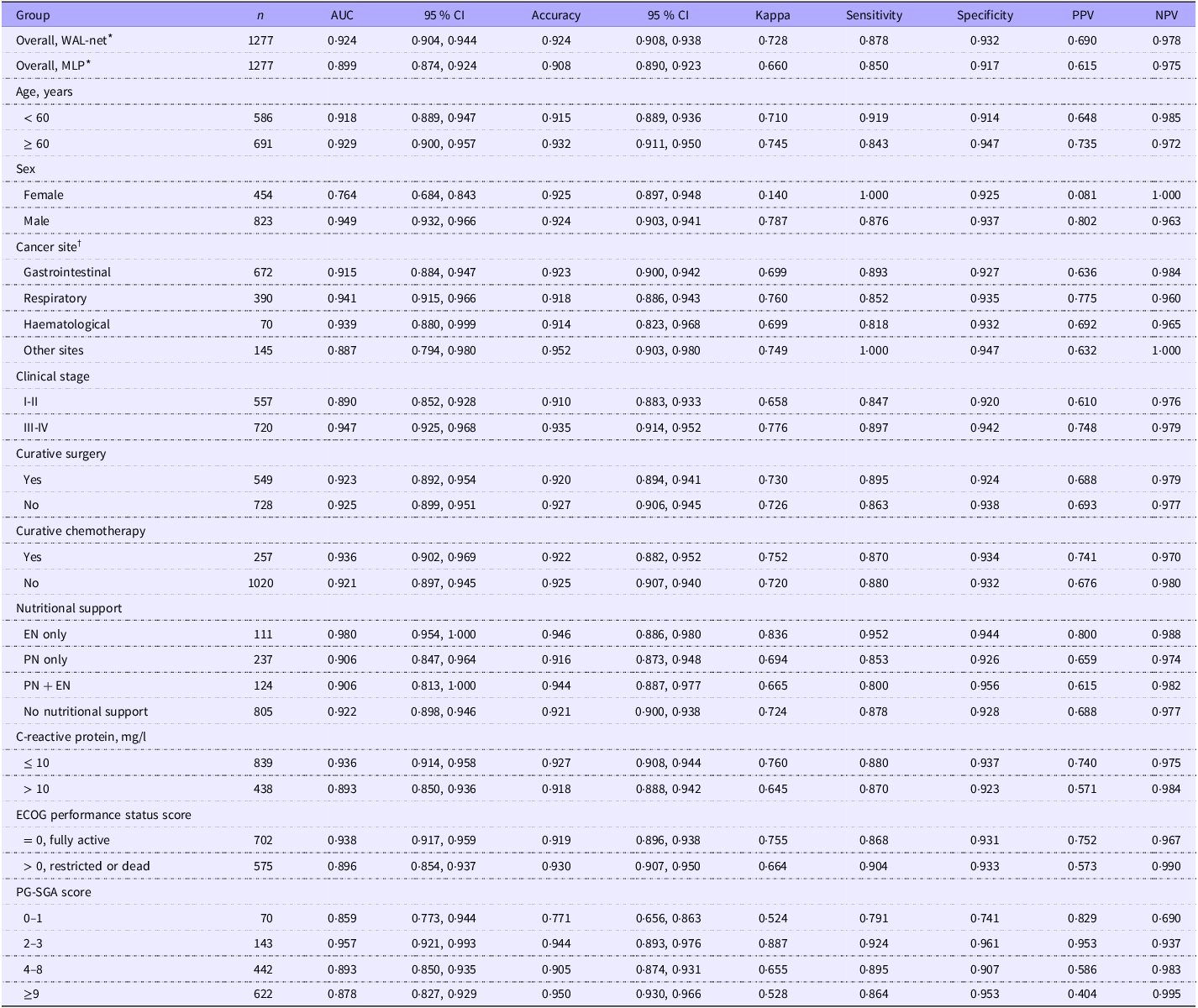
Subsequently, the WAL-net was trained in the discovery set and was compared with the MLP model in the holdout test set (Figure 3(c)–(d) and Table 2). The WAL-net showed higher performance (AUC = 0·924, 95 % CI = 0·904, 0·944) than the MLP model (AUC = 0·899, 95 % CI = 0·874, 0·924). A Delong’s test indicated that the AUC difference was statistically significant (P = 0·005). For other metrics, the WAL-net showed higher accuracy (0·924 v. 0·908), Kappa index (0·728 v. 0·660), sensitivity (0·878 v. 0·850), specificity (0·932 v. 0·917), positive predictive value (0·690 v. 0·615) and negative predictive value (0·978 v. 0·975) than the MLP model. Thus, the WAL-net was finally selected for future analysis as the state-of-the-art model in our specific task. The precision–recall curve, Kolmogorov–Smirnov statistic plot, cumulative gains curve, lift curve, calibration curve and confusion matrix and of the WAL-net in the test data are shown in Figure 4(a)–(f). The area and micro-average area under the precision–recall curve were 0·805 (class 1, the RM group) and 0·958, respectively (Figure 4(a)). The Kolmogorov–Smirnov statistic plot, cumulative gains curve, lift curve and calibration curve showed that the WAL-net has strong discrimination power and can effectively separate the positive and negative classes (Figure 4(b)–(e)). A Hosmer and Lemeshow goodness-of-fit test also supported the good consistency between model prediction and actual observation (P = 0·212, Figure 4(e)). The confusion matrix showed that there were 1015 (class 0, non-RM) and 165 (class 1, RM) patients who were correctly classified in the test data (Figure 4(f)).
Overall and subgroup model performance in the holdout test set

PPV, positive predictive value; NPV, negative predictive value; WAL, weight + appendicular skeletal muscle mass + long short-term memory; MLP, multilayer perceptron; PG-SGA, the patient generated subjective global assessment.
* WAL-net v. MLP, Delong’s test for AUCs, P = 0·005.
† Gastrointestinal system (colorectum, stomach, oesophagus, liver, pancreas, biliary tract and gastric stroma), respiratory system (lung and nasopharynx), haematological system (leukemia, lymphoma and multiple myeloma) other sites (cervix, ovary, endometrium, prostate, bladder, breast and brain).
Further evaluation of the WAL-net in holdout test data. (a) Precision–recall curve. (b) Kolmogorov –Smirnov statistic plot. (c) Cumulative gains curve. (d) Lift curve. (e) Calibration curve. (f) Confusion matrix.

Model performance in subgroups
The subgroup performance of the WAL-net was assessed in the test data (Table 2). Overall, the WAL-net sustained its good performance in different subgroups investigated. Specifically, by setting the AUC as the reference metric of model performance, the WAL-net showed relatively higher performance (defined as AUC > 0·950) in the subgroup of patients who only received enteral nutritional support (AUC = 0·980, 95 % CI = 0·954, 1·000) and patients with a PG-SGA score of 2 to 3 (AUC = 0·957, 95 % CI = 0·921, 0·993).
Model explainability
We evaluated the predictors of the WAL-net that contributed to the prediction on a global level. The SHAP summary plot showed that ASMI at baseline was the leading contributor to the high likelihood of RM, with a mean SHAP value of 1·590. In addition, the mean SHAP values for BMI, ASMI–1, ASMI–6, BMI–1 and BMI–6 were 0·806, 0·731, 0·417, 0·145 and 0·143, respectively (Figure 5(a)). We also examined the individual-level risk predictions and their sources of risk specified by the SHAP values. For the patient with the highest predicted SHAP value (e.g. 1), ASMI (0·69), BMI (0·11), BMI–1 (0·05), ASMI–1 (0·02), BMI–6 (0·02) and ASMI–6 (0·01) were the sources of risk that led to the high SHAP value (Figure 5(b)). On the other hand, for the patient with the lowest SHAP value (e.g. 0), BMI–6 (0·10), ASMI (–0·08), BMI–1 (–0·04), ASMI–6 (–0·04), ASMI–1 (–0·03) and BMI (–0·01) were the sources of risk that led to the low SHAP value (Figure 5(c)).
Interpretability analysis of the WAL-net using the shapley additive explanations (SHAP) method. ASMI, appendicular skeletal muscle mass index; −One, one month before baseline; −Six, six months before baseline. (a) Model interpretability at the group level. (b) Model interpretability at the individual level (high probability). (c) Model interpretability at the individual level (low probability).

Clinical relevance
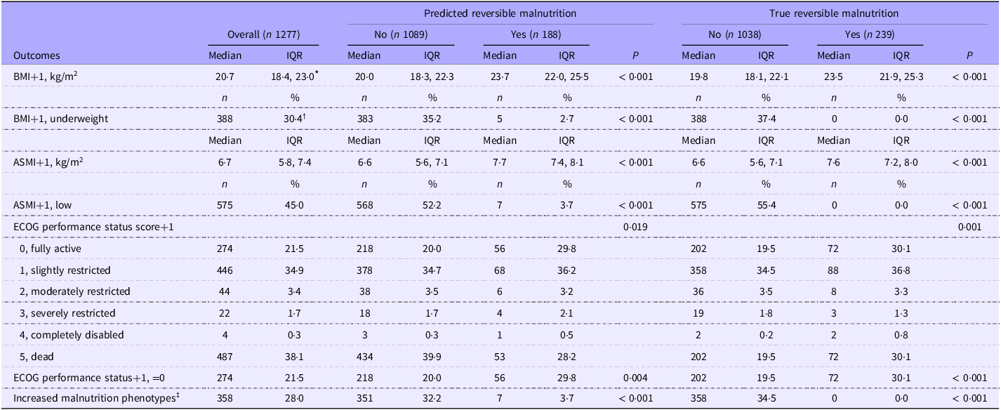
To examine the clinical relevance of the WAL-net, we analysed the associations of model-predicted RM with the clinical outcomes one month after admission (Table 3). Model-predicted RM was associated with higher values/rates of follow-up BMI and ASMI. Patients predicted as RM by the WAL-net at baseline were less likely to be classified in the underweight group and low muscle mass group one month after admission. In addition, patients with predicted RM were more likely to be classified in the normal physical performance one month after admission. Notably, the number of positive phenotypic criteria of GLIM were less likely to increase one month after admission in the RM group (all P < 0·05). Additionally, decision curve analysis analysis in the test set showed that if the threshold probability of a patient was > 0·01, using the WAL-net to predict the probability of RM adds more benefits than either the treat-all-patients scheme or the treat-none scheme (online Supplementary Figure S6).
Association of model prediction with short-term clinical outcomes in the holdout test set

Abbreviations: +1, one month after baseline; IQR, interquartile range; ASMI, appendicular skeletal muscle mass index; ECOG, the Eastern Cooperative Oncology Group.
* Median (interquartile range), all such values, compared using Wilcoxon’s rank-sum test.
† Number (percentage), all such values, compared using a χ 2d test.
‡ Defined as an increase in the number of positive malnutrition phenotypes (as diagnosed using the Global Leadership Initiative on Malnutrition framework) from baseline to one month after baseline (might be one to two or two to three).
Cutoff value for each input variable
To facilitate clinical use, the cut-offs (kg/m2) for the six input variables to predict RM were independently calculated in the discovery set (sex-specific cut-offs were calculated for ASMI) and then assessed in the test set (online Supplementary Table S5). For the three time points (–6, –1 and baseline), the BMI cut-offs were < 21·2, < 20·6 and < 18·5, respectively. Likewise, the ASMI cut-offs were men < 7·3 or women < 5·3, men < 7·0 or women < 5·3 and men < 7·1 or women < 5·3 for the three time points, respectively. After dichotomised using these cut-offs, the baseline BMI showed the highest prognostic value to predict RM in the test set (AUC = 0·771, 95 % CI = 0·739, 0·802).
Independent model validation
The WAL-net was further assessed for its classification power in the Yunnan cohort. Baseline characteristic of this cohort is shown in online Supplementary Table S6. RM was found in 106 (13·3 %) patients. The model’s good performance sustained, with an AUC (95% CI) = 0·909 (0·876, 0·943), accuracy (95 % CI) = 0·940 (0·921, 0·955), Kappa = 0·686, sensitivity = 0·953, specificity = 0·939, PPV = 0·575 and NPV = 0·996 (online Supplementary Table S7).
Model deployment
Prototypic applications were developed to utilise the WAL-net. These applications were designed to receive user input BMI and ASMI parameters and provide instant RM predictions. These applications deliver both the predicted class and the corresponding probability or confidence as outputs. The graphical user interface of the applications is presented in online Supplementary Figure S7. The serialised model objects that support future reuse and the application-related files have been stored online in our GitHub repository for public access (https://github.com/kevinlyy/rmalnutrition).
Discussion
In this study, we focused on addressing a significant real-world challenge regarding the reversibility of malnutrition in patients with cancer. To our knowledge, this is the first large-scale study that predicts RM using an explainable, long short-term memory-based deep learning model with high performance (AUC = 0·924). We have also confirmed an important hypothesis: the dynamic information of body weight and predicted appendicular skeletal muscle, which is routinely available upon patient admission, can independently predict the future trajectory of cancer-associated malnutrition. As our model does not require consideration of the treatment the patient will subsequently receive, this constitutes its ability for early identification. The findings underscore the importance of body weight and muscle mass surveillance within clinically operational timeframes for oncology patients. The model we developed, along with other findings presented in the study, might assist clinicians with decision-making to help guide more individualised management strategies of malnutrition in cancer care.
Compared with previous studies that only reported the baseline prevalence of GLIM-defined malnutrition in patients with cancer(Reference Yin, Song and Cui4,Reference Yin, Lin and Liu5) , the present study provides more clinically relevant information for decision-making by reporting the cancer-specific prevalence of RM (Figure 1(b)). Clinicians in oncology practice may typically prioritise cancer sites with higher incidence rates of malnutrition, such as pancreatic cancer(Reference Bouloubasi, Karayiannis and Pafili40) and gastrointestinal cancers(Reference Yaceczko and Baltz41). However, our observations revealed a distinct pattern in the reversibility of malnutrition across different cancer sites compared to their prevalence. For instance, prostate and brain cancer are generally associated with a low incidence of malnutrition(Reference Yin, Song and Cui4), but they exhibited higher rates of RM (Figure 1(b)). These findings underscore the importance of early identification and targeted management strategies, particularly for patients with RM in these specific cancer sites. Implementing such strategies increases the likelihood of achieving reversal and restoring weight/muscle mass(Reference Kipouros, Vamvakari and Kalafati15). In contrast, malnutrition in some cancers, such as those located in the biliary tract, ovary and esophagus, is more difficult to ameliorate (RM% < 10 %). This suggests that malnutrition occurring in these cancer sites is more refractory. These results (non-RM% of gastrointestinal cancers = 85·1 %) partially align with previous studies reporting the statistics of refractory cachexia in patients with cancer(Reference Zhou, Yang and Thapa42,Reference Nakajima43) , which showed that gastrointestinal cancers were the most refractory. A recent systematic review found that in patients with incurable solid cancer, nutritional intervention, either alone or as part of a multimodal approach, has improved quality of life, body weight and nutritional intake(Reference McLuskie, Bowers and Bayly44). Another review also indicated that multimodal interventions, including nutritional support, are effective in preventing unintentional weight loss in cancer patients(Reference Baguley, Edbrooke and Denehy45). These lines of evidence, along with our research findings, collectively suggest that for patients classified as non-RM, additional efforts and specialised interventions may be required to address the unique challenges associated with these cancers and potentially improve outcomes(Reference Nakajima43). Similarly, this decision strategy may also be applicable to the RM/non-RM status in the overall population. In this study, although the RM group received less nutritional support than the non-RM group, it was associated with improved nutrition-related outcomes. This implies that the RM/non-RM status predicted by the model might provide additional information to distinguish whether a malnourished patient is likely or unlikely to benefit from nutritional or multidisciplinary intervention. However, epidemiological statistics on cancer-specific prevalence of RM remain scare, especially those derived from Asian populations. As we only include malnourished patients, future studies should aggregate data on both cancer-specific malnutrition prevalence and RM prevalence within the same ethnic groups. Additionally, elucidating the underlying mechanisms behind the differing prevalence of RM in various cancer sites is crucial.
A potential drawback of the GLIM framework is that it does not provide overall nutritional/multidisciplinary treatment recommendations with respect to different malnutrition phenotypes and severities(Reference Cederholm, Jensen and Correia16). To inform treatment strategies for patients with GLIM-defined malnutrition, one possible solution is to refer to the cancer cachexia guideline(Reference Fearon, Strasser and Anker34), as malnutrition with inflammation and cachexia has been described as interchangeable concepts in some literature(Reference Cederholm, Barazzoni and Austin1,Reference Muscaritoli, Imbimbo and Jager-Wittenaar46) . Fearon’s framework for diagnosing cancer cachexia defines progressive stages of cachexia (from pre-cachexia to cachexia to refractory cachexia)(Reference Fearon, Strasser and Anker34). Early monitoring and preventive intervention are recommended for patients with pre-cachexia, as once cachexia is well established, treatment becomes more difficult(Reference Penet and Bhujwalla47). For patients at the cachexia stage, multimodal management according to phenotype is needed to prioritise those reversible contributory factors(Reference Fearon, Strasser and Anker34). For refractory cachexia, medical interventions may be futile or inappropriately invasive(Reference Arends, Bachmann and Baracos3,Reference Roeland, Bohlke and Baracos48) . However, it is important to note that although the diagnostic parameters used in Fearon’s framework(Reference Fearon, Strasser and Anker34) are the same as the phenotype criteria in the GLIM(Reference Cederholm, Jensen and Correia16), the cut-off values for specific variables such as weight loss and muscle loss differ. Additionally, other frameworks may employ different criteria for diagnosing cachexia(Reference Evans, Morley and Argiles49,Reference Argiles, Lopez-Soriano and Toledo50) . Therefore, treatment strategies applicable to the stages of cancer cachexia may not necessarily fully applicable to the different phenotypes and grades defined by GLIM. In contrast, our model was directly developed based on GLIM, making it more suitable for decision-making in the context of malnutrition. As the global recognition of GLIM continues to increase(Reference Barazzoni, Jensen and Correia27), our model is promising to serve as a useful tool to evaluate the burdens and costs of anti-malnutrition therapies against the expected benefits for patients.
Another noteworthy point to consider is that our findings reflect the real-world challenges that exist in current treatment strategies for cancer-associated malnutrition in China(Reference Xu, Song and Yin30). Even among patients diagnosed with malnutrition, the coverage rate of nutritional support remains low (36·9 %), and only a small proportion of malnourished patients can be reversed (17·7 %). We observed in our own practice that clinicians may instinctively prioritise patients with more severe malnutrition-related phenotypes, while these patients may face greater challenges in deriving benefits from nutritional support. Indeed, patients in the non-RM group exhibited a higher prevalence of various gastrointestinal symptoms, reduced food intake, nutritional risk, low BMI, impaired physical status, advanced cachexia stage, etc. However, despite a higher rate of nutritional support during hospitalisation in the non-RM group, there was no significant improvement in clinical benefits compared with the RM group. Because the severity of the primary disease, as indicated by the clinical tumor stage, is not significantly different between the non-RM and RM groups. It might be true that a diagnosis of malnutrition alone is insufficient to guide nutritional intervention strategies. A refined patient classification is necessary to provide guidance for more individualised treatment approaches. For example, create a staging system that reflects the pathophysiological progression of malnutrition and treatment response, rather than solely relying on the severity of phenotypic parameters. Another possible reason for the low rate of RM is the nutritional interventions in the present cohort were not strictly individualised and were not combined with other multimodal approaches such as physical exercise program, pharmacological interventions and psychological support(Reference Xu, Song and Yin30). Therefore, further studies in patients with individualised nutrition support data(Reference Schuetz, Fehr and Baechli51), especially multimodal anti-malnutrition data(Reference Arends, Bachmann and Baracos3), are imperative to provide greater insights regarding the clinical usefulness of the model.
The study has several potential limitations that must be noted. First, malnutrition and RM were both diagnosed using the GLIM framework that includes the weight loss as a major criterion. Because weight loss was calculated based on patient-reported historic weight data, the impact of recall bias on the classification of malnutrition and RM cannot be eliminated(Reference Yin, Cui and Lin39). Future studies with a prospective design and measured body weight values are needed to replicate our findings. Second, the ASMI was derived from an equation validated for use in Asians rather than measured using technologies such as dual energy X-ray imaging or bioimpedance analysis. However, the equation showed good consistency with dual energy X-ray imaging(Reference Wen, Wang and Jiang52), and body weight and height are simple to obtain in almost any institutions, which should increase the usability of the study parameters in different scenarios. Nevertheless, future studies using more advanced technologies to measure appendicular muscle mass are needed. Third, the model utilises weight and skeletal muscle dynamic information from three time points for predicting RM. Future studies need to investigate whether incorporating additional time points would result in further improvements in prediction performance. However, the weight loss information over past one and/or six months has been included in the most popular nutritional assessment tools which are easily accessible in oncology practice(Reference Cederholm, Jensen and Correia16,Reference Kondrup, Allison and Elia31,Reference Ottery32) , further increasing the generalisability of our model. Fourth, the present study only observed RM one month after baseline, future studies employ other time points are needed. Future studies with a larger sample size for a wider spectrum of diseases are needed to address the above issues.
Conclusion
In conclusion, we have provided the first report on the overall and cancer-specific prevalence of RM in a nationwide, multicenter cancer cohort. We have confirmed the hypothesis that the dynamic information of body weight and skeletal muscle, which is routinely available upon patient admission, can independently predict the future trajectory of malnutrition with high accuracy. We developed and validated an explainable deep learning model for the early identification of RM. This model utilises six easily accessible variables related to body weight and appendicular skeletal muscle dynamics, which showed good performance to predict RM. These findings might assist clinicians or nutritionists in decision-making to help guide management strategies of cancer-associated malnutrition and optimise the allocation of healthcare resources in cancer care.
Supplementary material
For supplementary material/s referred to in this article, please visit https://doi.org/10.1017/S000711452510384X
Acknowledgements
The authors would like to thank the Investigation on Nutrition Status and its Clinical Outcome of Common Cancers project members for their substantial work on data collection and patient follow-up.
This work was supported by the National Natural Science Foundation of China (82304131), the Natural Science Foundation of Chongqing, China (CSTB2024NSCQ-MSX1233), the Young Doctoral Talent Incubation Program of the Xinqiao Hospital, Army Medical University (2024YQB033) and the National Key Research and Development Program of China (2017YFC1309200).
L. Y.: Conceptualisation, methodology, software, data curation, writing – original draft preparation, funding acquisition and revising; N. L. and J. L.: Data curation and project administration; W. L., J. C., Z. G., Q. Y., F. Z., M. L., Z. C., H. Y., T. L., Z. L., P. J. and C. S.: Methodology, data curation and project administration; H. X.: Project administration, data curation, methodology and reviewing; H. S.: Conceptualisation, supervision, project administration, methodology, software and funding acquisition and reviewing.
The authors declare that they have no conflicts of interest.
Data described in the manuscript will not be made available because of multiple confidentiality agreements signed with participating hospitals.