1 Introduction
Double-diffusive convection has long been recognized as an important process responsible for the vertical exchange of heat and salinity in the oceans (Schmitt & Evane Reference Schmitt and Evane1978; Huppert & Turner Reference Huppert and Turner1981). When initially stable stratification is caused by two distinctive diffusive agents, according to Huppert & Turner (Reference Huppert and Turner1981), double-diffusive convection occurs as a result of flow instability in cases with a large fast-to-slow diffusivity ratio. A recent comprehensive theoretical study on double-diffusive convection can be found in Radko (Reference Radko2013), which shows that the instability depends upon the Prandtl number, the diffusivity ratio and the bulk density ratio between the two diffusive agents. In this rigidly stratified system, which is usually treated with an initial two-layer configuration, when a hot saline water column is above cold fresh water, convection occurs in the form of small (i.e., in the order of centimetres) structures known as salt fingers. This phenomenon has been studied extensively in laboratory experiments (Turner Reference Turner1967; Linden Reference Linden1973; Schmitt Reference Schmitt1979; Taylor & Bucens Reference Taylor and Bucens1989) and field observations (Schmitt Reference Schmitt1994; Schmitt et al. Reference Schmitt, Ledwell, Montgomery, Polzin and Toole2005).
If the upper water column contains fine suspended particles that result in excess bulk density, convective sedimentation can occur as a result of Rayleigh–Taylor instability (RTI) or double diffusion, also known as double-diffusive sedimentation. The discovery of double-diffusive sedimentation was first made in a laboratory tank experiment by Houk & Green (Reference Houk and Green1973) and further discussed in later studies (Green & Schettle Reference Green and Schettle1986; Green Reference Green1987) by the same group. These pioneering studies focused on simple scaling arguments and the analogy between sediment fingers and salt fingers. More systematic experimental studies (Chen Reference Chen1997; Hoyal, Bursik & Atkinson Reference Hoyal, Bursik and Atkinson1999; Parsons & Garcia Reference Parsons and Garcia2000) were later conducted to investigate particle fluxes in double-diffusive sedimentation. The resulting particle fluxes were found to be significantly greater than those induced by gravitational settling of individual particles. In addition, Hoyal et al. (Reference Hoyal, Bursik and Atkinson1999) developed a mathematical model to predict the enhanced sedimentation in the field. More recently, linear theories have been used to study double-diffusive sedimentation (Burns & Meiburg Reference Burns and Meiburg2012; Yu, Hsu & Balachandar Reference Yu, Hsu and Balachandar2013). These studies apply the equilibrium, scalar-limit approximation to describe the transport of the sediment concentration. The approximation leads to a scalar transport equation with the addition of vertical advection by the particle settling velocity calculated with Stokes’ law. The equilibrium condition (i.e., the addition of the settling velocity) is valid in the case of relatively fine particles (e.g.,  ${\sim}O(\unicode[STIX]{x03BC}\text{m})$) in natural water bodies (Chou, Wu & Shih Reference Chou, Wu and Shih2014a; Shao, Hung & Chou Reference Shao, Hung and Chou2017). A focus of these theoretical studies (Burns & Meiburg Reference Burns and Meiburg2012; Yu et al. Reference Yu, Hsu and Balachandar2013) was to distinguish two distinct mechanisms that can cause different types of instability at the sediment-laden interface: double diffusion and particle settling. The former is due to the transport of the rapid diffusive agent (e.g., heat), and the latter is due to the settling of groups of individual particles, which then forms a layer of reverse buoyancy, leading to RTI (Shao et al. Reference Shao, Hung and Chou2017), also known as settling instability. The same groups later conducted direct numerical simulations (DNS) (Yu, Hsu & Balachandar Reference Yu, Hsu and Balachandar2014; Burns & Meiburg Reference Burns and Meiburg2015) to investigate the dynamics of double-diffusive sedimentation for the nonlinear regime and the distinction between it and the convection induced by the settling instability.
Unlike the abundance of documentation for salt fingers, studies of sediment fingers remain relatively limited, probably because they are highly analogous with salt fingers. However, early experimental studies by Green & Schettle (Reference Green and Schettle1986), Chen (Reference Chen1997) suggested that sediment-laden fingers differ from salt fingers in that large caps or vortex rings can form at the tip of the sediment-laden fingers, whereas the downward diffusing component in salt fingers soon mixes thoroughly with the surrounding water. Described as a ‘striking difference’ between the two cases, a more specific discussion of the formation of the vortex ring associated with double-diffusive sediment fingers was presented by Green & Schettle (Reference Green and Schettle1986), who reported that ‘the fingers quickly form bulbous tips, which then separate from the parent finger, and develop into vortex rings’. These rings are unstable, and most of them develop two or three secondary rings. However, likely due to the limitations of the experimental apparatus, the discussion is rather qualitative and phenomenological. The differences between the salt fingers and sediment fingers are due to the negligible diffusivities in the latter. For example, the particle size that can maintain long-term suspension in natural water bodies usually ranges from  $O(1~\unicode[STIX]{x03BC}\text{m})$ to
 $O(100~\unicode[STIX]{x03BC}\text{m})$, and based on the Einstein–Stokes equation, the diffusivity
 $\unicode[STIX]{x1D705}_{\unicode[STIX]{x1D719}}$ for the spherical particle of diameter
 $d_{0}=5~\unicode[STIX]{x03BC}\text{m}$ is approximately
 $10^{-14}~\text{m}^{2}~\text{s}^{-1}$ and decreases as the particle size increases. As a result of the low diffusivity, the descending mass of the slowly diffusive agent can be more easily retained within the finger because of the lower diffusive flux; this phenomenon is discussed in greater detail in § 7. Moreover, one can examine the instability criterion for the two cases by looking at the diffusivity ratio
 $R_{\unicode[STIX]{x1D705}}=\unicode[STIX]{x1D705}_{T}/\unicode[STIX]{x1D705}_{\unicode[STIX]{x1D719}}$ in the thermal-sediment system, where
 $\unicode[STIX]{x1D705}_{T}$ is the diffusivity of temperature. For the typical saline-thermal system in the ocean, the diffusivity ratio between temperature and salinity is slightly greater than 100, which leads to double-diffusive convection (Huppert & Turner Reference Huppert and Turner1981; Radko Reference Radko2013). In the same bulk conditions, the greater
 $R_{\unicode[STIX]{x1D705}}$, due to the lower diffusivity of sediment, warrants double-diffusive convection in the thermal-sediment system; moreover, without excessive molecular diffusion, the low
 $\unicode[STIX]{x1D705}_{\unicode[STIX]{x1D719}}$ value may result in more rigorous mass transport (i.e., convective flux). Unfortunately, due to the difficulties in achieving the actual low diffusivities in numerical discretization, the scalar-limit approximation adopted for DNS in recent numerical studies (Yu et al. Reference Yu, Hsu and Balachandar2014; Burns & Meiburg Reference Burns and Meiburg2015) were not capable of resolving the differences between the two, although high-resolution simulations enabled investigation of important flow structures in great detail.
A main objective of studying sediment fingers in double diffusion is to understand the hydrodynamic mechanism that can enhance vertical transport of suspended materials in natural water bodies such as oceans. Studies (Parsons, Bush & Syvitski Reference Parsons, Bush and Syvitski2001; Hizzett et al. Reference Hizzett, Hughes Clarke, Sumner, Cartigny, Talling and Clare2018) have shown that settling of sediment plumes descending from the turbid layer at the ocean surface plays a major role in the formation of underwater turbidity currents, which are responsible for changing seabed bathymetry. Double-diffusive sedimentation has been recognized as an important mechanism in the enhancement of settling of suspended particles from the surface plume. Moreover, it can serve as an active mechanism to accelerate the downward transport of aggregated microorganisms from the ocean surface to the ocean bottom, as known as ‘marine snow’, which is the foundation of the deep-sea ecosystem (Alldredge & Cohen Reference Alldredge and Cohen1987). Marine snow also provides an important path for the transportation of carbon dioxide from the surface to the deep ocean, which is a key mechanism in enhancing carbon sequestration in the ocean. Although the contribution of double-diffusive sedimentation, relative to particle aggregation, to the generation of marine snow remains unclear, a more detailed study of particle-laden fingers in double-diffusive sedimentation can be a first step in advancing our current understanding. In the present study, using Lagrangian particle tracking to simulate the motion of a considerable number of suspended particles along with DNS for flow motion, we aim to reveal the detailed flow dynamics and plume structures via high-resolution numerical studies. Compared with the previous DNS studies in conjunction with the scalar-limit assumption for sediment (Yu et al. Reference Yu, Hsu and Balachandar2014; Burns & Meiburg Reference Burns and Meiburg2015), the Lagrangian approach does not suffer from artificial diffusion due to the mesh size restriction in the continuous approach. To our knowledge, this is the first time that the Eulerian–Lagrangian (EL) approach has been successfully applied in the study of double-diffusive sediment fingers. In addition to replicating the features realized in early experimental studies, a detailed investigation of plume geometry and structure allows us to present a simple theoretical model for prediction of the descending speed of plume heads. Moreover, numerical experiments on various particle sizes and the scalar-limit assumption allow a detailed discussion of the effect of particle size and diffusivity, both of which have critical importance in distinguishing the dynamics of salt and particle-laden fingers.
The rest of the paper is outlined as follows. Section 2 presents the mathematical formulation, numerical methods, simulation set-up, and relevant scaling parameters. In § 3, we present the numerical results and a qualitative discussion of the formation of the sediment-laden drop and the subsequent vortex ring. This section also demonstrates consistency with the early experimental studies (Green & Schettle Reference Green and Schettle1986). In § 4, based on the numerical results, we propose a simple drag model of the slowly descending drop and show good agreement in predicting the speed of the particle-laden drop. Section 5 presents our analysis of various particle sizes, in which we restrict our discussion to particles that are not large enough to intervene in the features of double diffusion fingers. To demonstrate the predictability of our drag model, § 6 presents the application of the theoretical model derived in § 4 to predict the speed of descending particle-laden drops in cases with various simulation conditions and the previous experimental results. The effects of diffusivity are then discussed in § 7, which presents the distinction between the salt and particle-laden fingers in forming the drop and ring. Our concluding remarks are then given in § 8.
2 Method
2.1 Governing equations
We consider hydrodynamic drag and gravitational force to describe particle motion. The momentum of a single solid particle is thus described as
 $$\begin{eqnarray}m_{p}\frac{\text{d}\boldsymbol{u}_{p}}{\text{d}t}=m_{p}\frac{\boldsymbol{u}_{c|p}-\boldsymbol{u}_{p}}{\unicode[STIX]{x1D70F}_{p}}+(m_{p}-m_{f})\boldsymbol{g},\end{eqnarray}$$
where  $m_{p}$ is the mass of the solid particle,
 $m_{f}$ is the mass of the fluid,
 $\text{d}/\text{d}t$ is the material derivative of the Lagrangian particle moving with a velocity
 $\boldsymbol{u}_{p}$,
 $\boldsymbol{u}_{c|p}$ is the velocity of the continuum phase evaluated at particle location
 $\boldsymbol{x}_{p}$,
 $\boldsymbol{g}$ is the gravitational acceleration and
 $\unicode[STIX]{x1D70F}_{p}$ is the particle relaxation time, which can be obtained with (Schiller & Nauman Reference Schiller and Nauman1935)
 $$\begin{eqnarray}\unicode[STIX]{x1D70F}_{p}=\frac{\unicode[STIX]{x1D70C}_{p}}{\unicode[STIX]{x1D70C}_{0}}\frac{d_{p}^{2}}{18\unicode[STIX]{x1D708}}(1+0.15Re_{p}^{0.687})^{-1}\end{eqnarray}$$
in which  $\unicode[STIX]{x1D70C}_{p}$ and
 $\unicode[STIX]{x1D70C}_{0}$ are densities of the particle and fluid phases, respectively,
 $d_{p}$ is the particle diameter,
 $\unicode[STIX]{x1D708}$ is the kinematic viscosity and
 $$\begin{eqnarray}Re_{p}=\frac{|\boldsymbol{u}_{c|p}-\boldsymbol{u}_{p}|d_{p}}{\unicode[STIX]{x1D708}}\leqslant 800\end{eqnarray}$$
is the particle Reynolds stress. For the fluid phase, we consider a density stratified incompressible flow subject to the drag force due to a certain number of point particles. Under the Boussinesq approximation, the momentum equations are written as
 $$\begin{eqnarray}\frac{\unicode[STIX]{x2202}\boldsymbol{u}_{c}}{\unicode[STIX]{x2202}t}+\boldsymbol{u}_{c}\boldsymbol{\cdot }\unicode[STIX]{x1D735}\boldsymbol{u}_{c}=-\frac{1}{\unicode[STIX]{x1D70C}_{0}}\unicode[STIX]{x1D735}p+\unicode[STIX]{x1D708}\unicode[STIX]{x1D6FB}^{2}\boldsymbol{u}_{c}+\boldsymbol{f}-\unicode[STIX]{x1D6FC}\left(T-T_{r}\right)\boldsymbol{g},\end{eqnarray}$$
where the subscript  $c$ indicates the continuous phase,
 $p$ is the dynamic pressure,
 $\boldsymbol{f}$ is the total drag exerted by the particles on the fluid,
 $T$ is the temperature,
 $T_{r}$ is the reference temperature and
 $\unicode[STIX]{x1D6FC}$ is the density expansion coefficient of the temperature. Mass conservation of the fluid phase is governed by the continuity equation
 $$\begin{eqnarray}\unicode[STIX]{x1D735}\boldsymbol{\cdot }\boldsymbol{u}_{c}=0.\end{eqnarray}$$
Transport of the temperature field,  $T$, is governed by the advection–diffusion equation, i.e.,
 $$\begin{eqnarray}\frac{\unicode[STIX]{x2202}T}{\unicode[STIX]{x2202}t}+\boldsymbol{u}_{c}\boldsymbol{\cdot }\unicode[STIX]{x1D735}T=\unicode[STIX]{x1D705}_{T}\unicode[STIX]{x1D6FB}^{2}T,\end{eqnarray}$$
where  $\unicode[STIX]{x1D705}_{T}$ is the diffusion coefficient for the temperature. In the present study, we consider the diluted condition for suspended particles (volume fraction
 ${<}1\,\%$) so that the Boussinesq approximation is applied. The forcing term
 $\boldsymbol{f}$ in (2.4) within a control volume for monodispersed particles is obtained with
 $$\begin{eqnarray}\boldsymbol{f}=-r_{\unicode[STIX]{x1D70C}}\mathop{\sum }_{k=1}^{N_{p}}\{_{p}\frac{\boldsymbol{u}_{c|p,k}-\boldsymbol{u}_{p,k}}{\unicode[STIX]{x1D70F}_{p}},\end{eqnarray}$$
where  $N_{p}$ is the total number of particles in the control volume,
 $\{_{p}$ is the volume fraction of a single particle and
 $r_{\unicode[STIX]{x1D70C}}=\unicode[STIX]{x1D70C}_{p}/\unicode[STIX]{x1D70C}_{0}$.
2.2 Rationality of the model
Equation (2.1) is a simplified equation that describes particle motion in a fluid. For a more complete description of hydrodynamic forcing terms with coefficients whose magnitude  ${\geqslant}O(d_{p})$, the added mass and pressure effects should be considered in addition to (2.1). That is, along with the particle stresses due to collision, the momentum of a single solid particle can be described as (Maxey & Riley Reference Maxey and Riley1983; Ferry & Balachandar Reference Ferry and Balachandar2001)
 $$\begin{eqnarray}m_{p}\frac{\text{d}\boldsymbol{u}_{p}}{\text{d}t}=m_{p}\frac{\boldsymbol{u}_{c|p}-\boldsymbol{u}_{p}}{\unicode[STIX]{x1D70F}_{p}}+(m_{p}-m_{f})\boldsymbol{g}+C_{vm}m_{f}\left(\left.{\displaystyle \frac{\text{D}\boldsymbol{u}_{c}}{\text{D}t}}\right|_{p}-{\displaystyle \frac{\text{d}\boldsymbol{u}_{p}}{\text{d}t}}\right)-m_{f}\unicode[STIX]{x1D735}p+\boldsymbol{R}_{col},\end{eqnarray}$$
where  $\text{D}/\text{D}t$ is the material derivative following the fluid parcel,
 $C_{vm}$ is the added mass coefficient and
 $\boldsymbol{R}_{col}$ is the particle stress due to particle collision. As presented by Chou, Gu & Shao (Reference Chou, Gu and Shao2015), in a two-way coupled framework, solutions of (2.8) that consider the three additional forcing terms to (2.1) typically lead to a significantly extra computational load. However, theoretical derivations and numerical studies in a serial study by Chou et al. (Reference Chou, Wu and Shih2014a) and Chou, Wu & Shih (Reference Chou, Wu and Shih2014b) showed that for typical buoyancy-driven flows (i.e., RTI), added mass and pressure effects are important only when the volume concentration exceeds
 $O(0.01)$. As presented below, here we consider particle concentrations much below
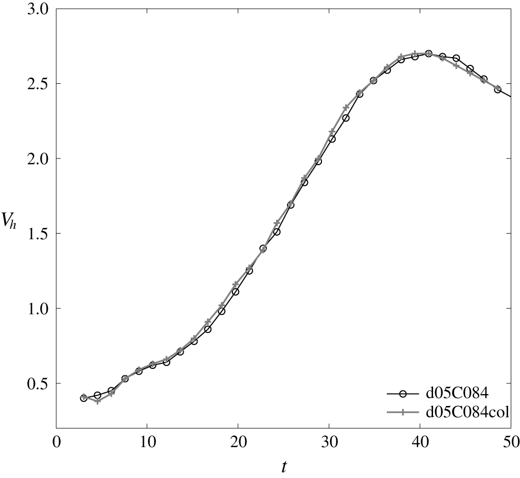
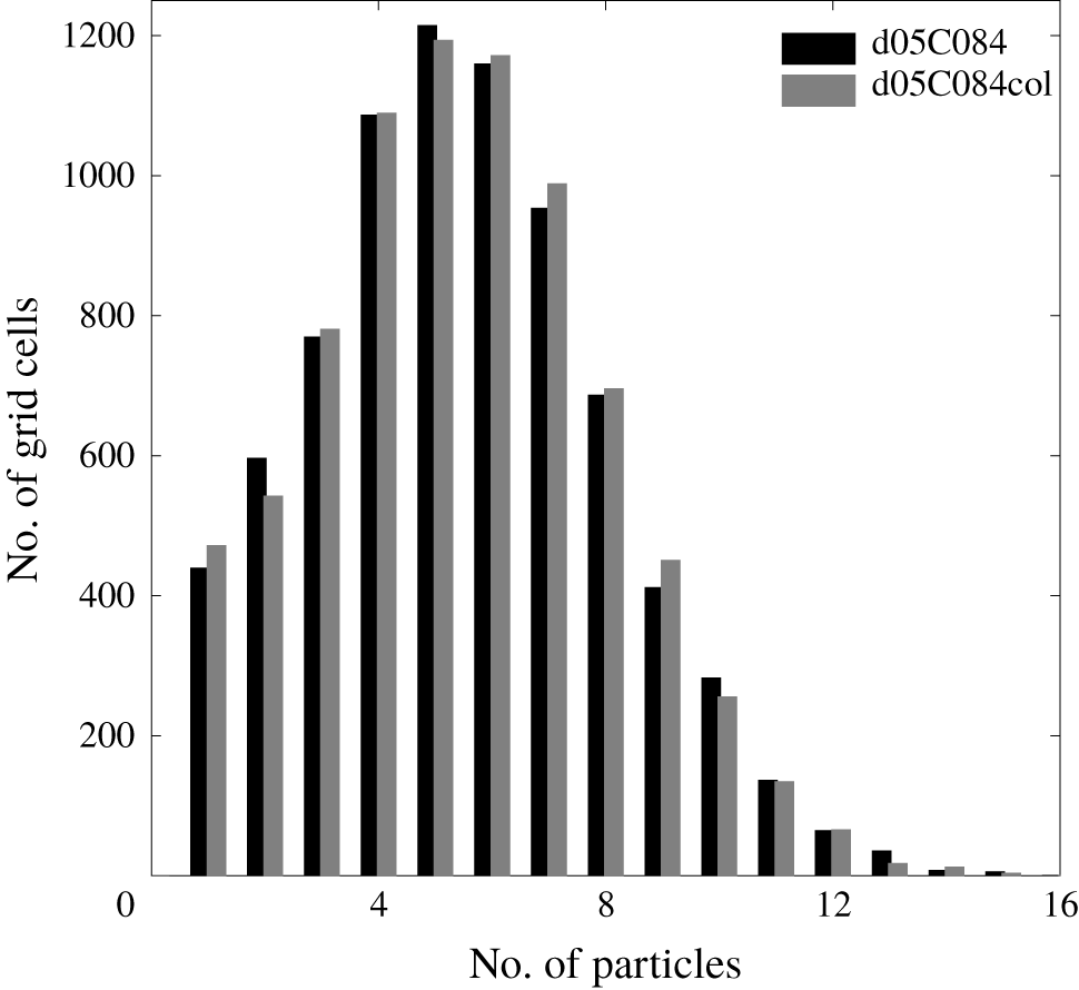
 $O(0.01)$ in volume fraction. Moreover, as we present in appendix A, the effect of particle collision is insignificant in bulk dynamics and particle distributions, which is consistent with the argument by Elghobashi & Truesdell (Reference Elghobashi and Truesdell1993) and Balachandar & Eaton (Reference Balachandar and Eaton2010) in the context of turbulent dispersed two-phase flow. Therefore, for the sake of computational efficiency and in consideration of their insignificant effect in the present concentration range, we disregard the added mass, pressure effect and particle–particle interaction (e.g., collision and coagulation) and apply the rather simplified version, equation (2.1), to model the motion of particles.
In fact, for the case in which  $\unicode[STIX]{x1D70F}_{p}$ is small such that the particle Stokes number
 $St=\unicode[STIX]{x1D70F}_{p}/\unicode[STIX]{x1D70F}_{f}\ll 1$ (in which
 $\unicode[STIX]{x1D70F}_{f}$ is the time scale of the flow), particle inertia becomes relatively small, and (2.1) can be simplified to
 $$\begin{eqnarray}\boldsymbol{u}_{p}\approx \boldsymbol{u}_{c|p}+\unicode[STIX]{x1D70F}_{p}\boldsymbol{g}^{\prime },\end{eqnarray}$$
where  $\boldsymbol{g}^{\prime }=\left(1-1/r_{\unicode[STIX]{x1D70C}}\right)\boldsymbol{g}$ is the reduced gravity and the second term on the right-hand side of (2.9) is also known as the settling velocity. Substitution of (2.9) for each
 $k$th particle into (2.7) and further substitution into (2.4) results in the momentum equations
 $$\begin{eqnarray}\frac{\unicode[STIX]{x2202}\boldsymbol{u}_{c}}{\unicode[STIX]{x2202}t}+\boldsymbol{u}_{c}\boldsymbol{\cdot }\unicode[STIX]{x1D735}\boldsymbol{u}_{c}=-\frac{1}{\unicode[STIX]{x1D70C}_{0}}\unicode[STIX]{x1D735}p+\unicode[STIX]{x1D708}\unicode[STIX]{x1D6FB}^{2}\boldsymbol{u}_{c}+\unicode[STIX]{x1D6FE}\unicode[STIX]{x1D719}\boldsymbol{g}-\unicode[STIX]{x1D6FC}(T-T_{r})\boldsymbol{g},\end{eqnarray}$$
where  $\unicode[STIX]{x1D6FE}=r-1$ and
 $\unicode[STIX]{x1D719}=N_{p}\unicode[STIX]{x1D719}_{p}$ is the total volume fraction of particles in the control volume (e.g., the grid cell) and, according to (2.9), its governing equation can be written in the Eulerian manner as
 $$\begin{eqnarray}{\displaystyle \frac{\unicode[STIX]{x2202}\unicode[STIX]{x1D719}}{\unicode[STIX]{x2202}t}}+\boldsymbol{u}_{c}\boldsymbol{\cdot }\unicode[STIX]{x1D735}\unicode[STIX]{x1D719}-W_{s}{\displaystyle \frac{\unicode[STIX]{x2202}\unicode[STIX]{x1D719}}{\unicode[STIX]{x2202}z}}=0,\end{eqnarray}$$
where  $W_{s}=\unicode[STIX]{x1D70F}_{p}g^{\prime }$. That is, under the near equilibrium condition that particle drags are soon in balance with the gravitational force (i.e.,
 $St\ll 1$), the present model formulation, equations (2.1) and (2.4)–(2.7) recover to the standard equilibrium Eulerian formulation, equations (2.10) and (2.11), that is frequently used in the community (e.g., Yu et al. Reference Yu, Hsu and Balachandar2014; Burns & Meiburg Reference Burns and Meiburg2015), except that transport of the concentration field is associated with zero diffusivity here.
Based on the estimation using the Einstein–Stokes equation, in which the particle diameters for this study are  $O(1{-}10~\unicode[STIX]{x03BC}\text{m})$, the diffusivities for their concentration fields are approximately
 $10^{-14}~\text{m}^{2}~\text{s}^{-1}$ or less, which are much smaller than the kinematic viscosity of water and the diffusivity of temperature. Although it has been found that the long-range correlation between concentration fluctuations of suspended particles can create ‘hydrodynamic diffusivity’ that significantly exceeds the molecular diffusivity (Segre et al. Reference Segre, Liu, Umbanhowar and Weitz2001), the applicability of such models to continuum representation for suspended sediment problems still requires further study of the parametric space and flow conditions that are more relevant to natural water flows. Moreover, because the hydrodynamic diffusivities are statistical quantities (i.e., statistical sampling of concentration fluctuations), its compatibility with DNS, which typically represents a flow realization, remains questionable and may require careful examination. Therefore, because realistically small values of molecular diffusivities are extremely difficult to obtain with the numerical solution of the advection–diffusion equation, the present Lagrangian-particle tracking approach provides a suitable alternative to the conventional Eulerian approach (e.g., equation (2.11) along with diffusivity) to model transport of fine suspended sediments, despite its high demand for computation.
The present transport equation of temperature, equation (2.6), assumes that particles are in their thermal equilibrium state such that no sink or source terms that arise from non-equilibrium thermal conduction of particles are considered. This assumption can be verified by estimating the time scale of heat conduction for an individual solid particle in this study. Given the thermal conductivity  $K_{s}\approx 0.15~\text{W}~{\text{m}^{-1}~}^{\circ }\text{K}^{-1}$ and heat capacity
 $c_{p}\approx 800~\text{J}~{\text{kg}^{-1}~}^{\circ }\text{K}^{-1}$ for sand grains (Hamdhan & Clarke Reference Hamdhan and Clarke2010), the time scale for heat conduction can be estimated by
 $\unicode[STIX]{x1D70C}_{p}c_{p}d_{p}^{2}/K_{s}$, which, for the present particle sizes, is
 $O(10^{-3}~\text{s})$ or less, which is much smaller than the present diffusion time scale (
 $O(10^{-1}~\text{s})$) (see § 2.4). Therefore, it is fair to assume that particles are in thermal equilibrium with the ambient flows and, in the transport equation of temperature, to neglect the additional thermal sink or source that arises from the non-equilibrium thermal conduction of particles.
2.3 Numerical methods
Calculations of particle momentum and movement are implemented in an incompressible Navier–Stokes solver originally developed by Zang, Street & Koseff (Reference Zang, Street and Koseff1994). In this code, a finite-volume method is used to discretize the governing equations on non-staggered grids. All spatial derivatives except the convective terms are discretized with second-order central differences. The convective terms are discretized using a variation of QUICK (Leonard Reference Leonard1979; Perng & Street Reference Perng and Street1989). For time advancement, the second-order Crank–Nicolson scheme is used for the diagonal viscous terms, and the second-order Runge–Kutta (RK2) method is used for all other terms. Following Kim & Moin (Reference Kim and Moin1985), the momentum equation is advanced with a predictor–corrector procedure based on the fractional-step method (Chorin Reference Chorin1968), in which a divergence-free velocity field is calculated at each time step by correcting the predicted velocity with the pressure gradient. The original single-phase code was successfully applied to simulations of numerous flow problems including turbulent lid-driven cavity flow (Zang et al. Reference Zang, Street and Koseff1994), coastal upwelling (Zang & Street Reference Zang and Street1995; Cui & Street Reference Cui and Street2004), interfacial waves (Fringer & Street Reference Fringer and Street2003; Venayagamoorthy & Fringer Reference Venayagamoorthy and Fringer2007; Arthur & Fringer Reference Arthur and Fringer2014), and sediment transport (Zedler & Street Reference Zedler and Street2001, Reference Zedler and Street2006; Chou & Fringer Reference Chou and Fringer2008, Reference Chou and Fringer2010). Calculation of particle movement was implemented by Chou et al. (Reference Chou, Gu and Shao2015), who also calculated the particle momentum using RK2, whereas its movement was performed with the explicit Euler method. In Chou et al. (Reference Chou, Gu and Shao2015), calculation of Lagrangian particles was validated by some canonical cases of suspended sediment transport. The present EL model has been applied to study particle-induced RTI (Chou & Shao Reference Chou and Shao2016). In this study, following Chou & Shao (Reference Chou and Shao2016), direct numerical simulation and point-force representation for fine suspended particles are employed to study double-diffusive sedimentation.
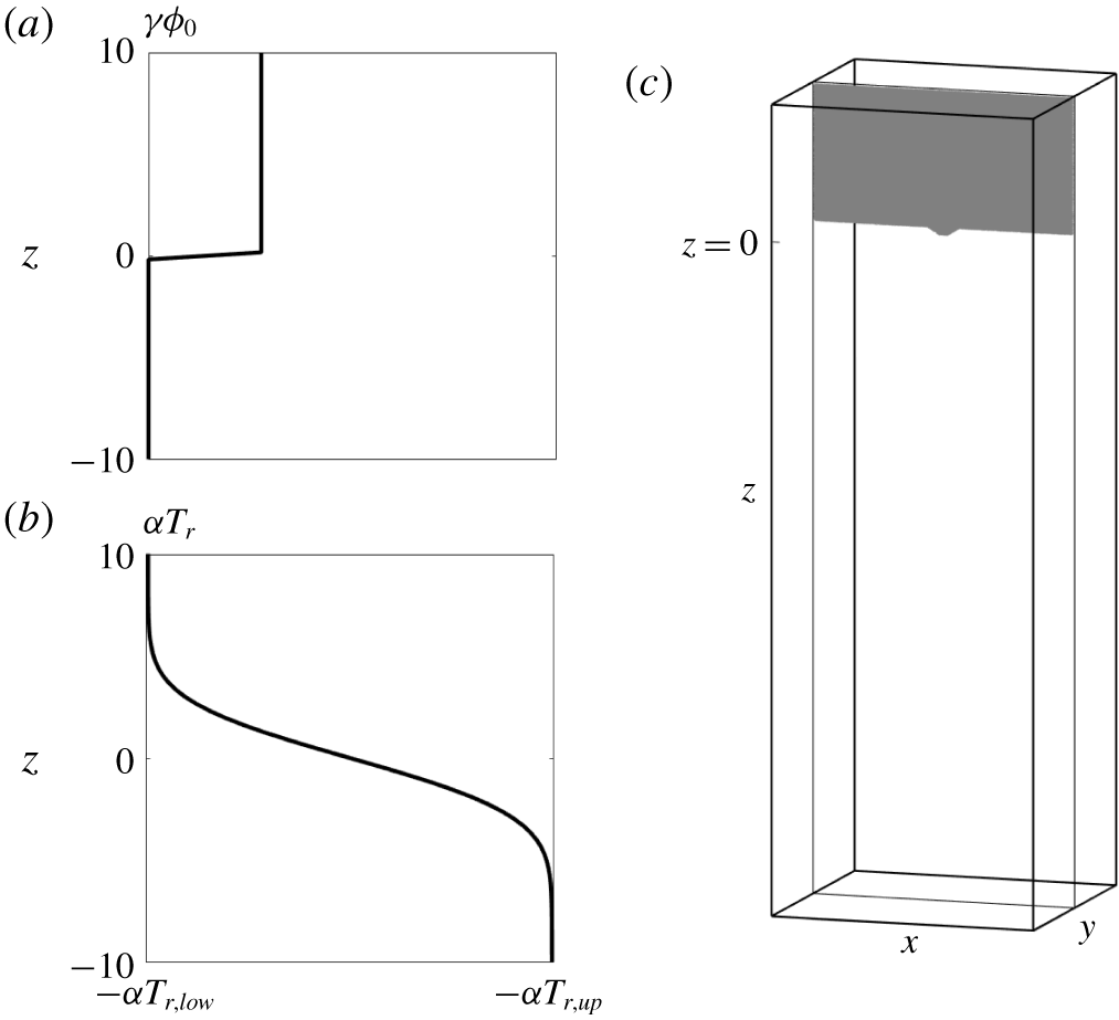
The profile of the density anomaly due to suspended particles (a), the profile of background density due to the reference temperature ( $T_{r}$) (b), and the domain configuration along with the initial distribution of particles (grey region) at the central slice in the
 $y$-direction.

2.4 Simulation set-up
As shown in figure 1(a), the simulation begins by assigning a particle-laden layer in the upper region of the domain, in which the flow is stably stratified due to a background temperature distribution ( $T_{r}(z)$) initially given by
 $$\begin{eqnarray}T_{r}(z)=T_{r,low}+0.5(T_{r,up}-T_{r,low})\left[1-\text{erf}\left({\displaystyle \frac{z}{l_{0}}}\right)\right],\end{eqnarray}$$
where  $z$ is the vertical coordinate,
 $l_{0}$ indicates the thickness of the interface and
 $T_{r,up}$ and
 $T_{r,low}$ are the reference temperatures at the upper and lower uniform regions, respectively. Following the experimental set-up in Green & Schettle (Reference Green and Schettle1986), we use
 $T_{r,up}=40.1\,^{\circ }\text{C}$ and
 $T_{r,low}=16.0\,^{\circ }\text{C}$. In (2.12),
 $l_{0}=4.5\times 10^{-4}~\text{m}$ is used to mimic the initial sharp density gradient between the two uniform-temperature layers in the laboratory set-up. Based on theories of double-diffusive convection (Radko Reference Radko2013), the length, time and velocity are, respectively, expressed in terms of the following dimensional quantities:
 $$\begin{eqnarray}L=\left({\displaystyle \frac{\unicode[STIX]{x1D705}_{T}\unicode[STIX]{x1D708}}{g\unicode[STIX]{x1D6FC}{\displaystyle \frac{\unicode[STIX]{x2202}T_{r}}{\unicode[STIX]{x2202}z}}}}\right)^{1/4},\quad \unicode[STIX]{x1D70F}={\displaystyle \frac{L^{2}}{\unicode[STIX]{x1D705}_{T}}},\quad U={\displaystyle \frac{\unicode[STIX]{x1D705}_{T}}{L}},\end{eqnarray}$$
where  $g$ is gravity,
 $\unicode[STIX]{x1D6FC}$ is the density expansion coefficient of the temperature,
 $\unicode[STIX]{x1D708}$ is the kinematic viscosity of water and
 $\unicode[STIX]{x1D705}_{T}$ is the diffusivity of temperature. In the present simulations, although
 $\unicode[STIX]{x2202}T_{r}/\unicode[STIX]{x2202}z$ slowly changes over time due to diffusion, for the sake of convenience, we use its initial value to obtain
 $L$. In this study,
 $\unicode[STIX]{x1D6FC}=2.07\times 10^{-4}$,
 $\unicode[STIX]{x1D708}=10^{-6}~\text{m}^{2}~\text{s}^{-1}$ and
 $\unicode[STIX]{x1D705}_{T}=1.5\times 10^{-7}~\text{m}^{2}~\text{s}^{-1}$, which gives
 $L=2.22\times 10^{-4}~\text{m}$,
 $U=6.75\times 10^{-4}~\text{m}~\text{s}^{-1}$ and
 $\unicode[STIX]{x1D70F}=3.30\times 10^{-1}~\text{s}$. In (2.13),
 $\unicode[STIX]{x2202}T_{r}/\unicode[STIX]{x2202}z$ is the gradient of the reference temperature measured at the initial position of the unperturbed particle-laden interface (i.e.,
 $z=0$).
As shown in figure 1(c), simulations are carried out in a three-dimensional domain sized  $L_{x}\times L_{y}\times L_{z}=90\times 90\times 270$, with gravitational forcing acting in the
 $z$-direction. The domain width allows for the lateral development of single-mode drop (i.e., vortex rings) in the present study, and the height allows the drop to reach its acceleration, terminal speed, and deceleration stages. The grid resolution is
 $256\times 256\times 768$. The periodic boundary condition is applied to all horizontal boundaries, and the free- and no-slip boundary conditions are applied to the upper and lower boundaries, respectively. Following Green & Schettle (Reference Green and Schettle1986), we begin the EL simulations of the base case by assigning particles in each grid cell according to the given bulk volume concentration,
 $\unicode[STIX]{x1D719}_{0}=8.40\times 10^{-4}$, but with random positions within that cell. In terms of the bulk density ratio between the two agents defined as
 $$\begin{eqnarray}R_{\unicode[STIX]{x1D70C}}={\displaystyle \frac{\unicode[STIX]{x1D6FC}\unicode[STIX]{x0394}T_{r}}{\unicode[STIX]{x1D6FE}\unicode[STIX]{x1D719}_{0}}},\end{eqnarray}$$
in which  $\unicode[STIX]{x0394}T_{r}=T_{r,up}-T_{r,low}$, the set-up of the base case gives
 $R_{\unicode[STIX]{x1D70C}}=3.60$. The interface between the particle-laden layer and the clear fluid is located at
 $45$ non-dimensional length units below the top boundary, which is the point at which
 $z=0$ is defined (see figure 1b,c). We choose five particle diameters,
 $d_{0}=3$,
 $5$,
 $7$,
 $10$ and
 $14~\unicode[STIX]{x03BC}\text{m}$, among which
 $d_{0}=5~\unicode[STIX]{x03BC}\text{m}$ serves as the base case for the following demonstration. In addition, cases with various
 $\unicode[STIX]{x1D719}_{0}$ and initial temperature differences are also simulated to test the predictability of the present theoretical model. We adopt the convention that each case is named by the combination of the two digits of the particle size
 $d_{p}$ (in
 $\unicode[STIX]{x03BC}\text{m}$) following the letter ‘d’ and three digits of bulk volume concentration (in parts per ten thousand) following the letter ‘C’. For the two additional cases with a different temperature set-up (see § 6 for more details), ‘T2’ is added to the end of the case name, as summarized in table 1. The specific density of each particle is 2.65, and the particle relaxation times,
 $\unicode[STIX]{x1D70F}_{p}$, based on Stokes’ law are
 $1.33\times 10^{-6}$,
 $3.68\times 10^{-6}$,
 $7.36\times 10^{-6}$,
 $1.47\times 10^{-5}$ and
 $2.88\times 10^{-5}~\text{s}$, respectively. This gives the particle Stokes number
 $St=\unicode[STIX]{x1D70F}_{p}/\unicode[STIX]{x1D70F}\ll 1$ in all cases, indicating that particle inertia is not important in the present study. In this case, equation (2.9) is a valid approximation, and the non-dimensional settling velocity
 $$\begin{eqnarray}w_{s}={\displaystyle \frac{W_{s}}{U}}={\displaystyle \frac{\unicode[STIX]{x1D70F}_{p}g^{\prime }}{U}}\end{eqnarray}$$
is used to indicate the particle size in each case hereafter. The five particle sizes (from small to large) correspond to  $w_{s}=1.20\times 10^{-2}$,
 $3.33\times 10^{-2}$,
 $6.67\times 10^{-2}$,
 $1.33\times 10^{-1}$ and
 $2.67\times 10^{-1}$.
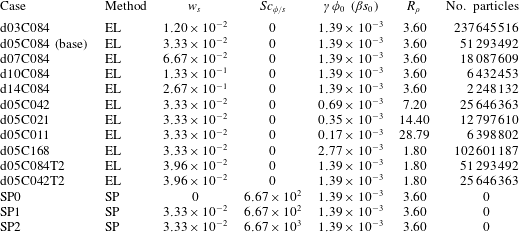
Physical parameters in the present simulation cases. Here EL indicates Eulerian–Lagrangian simulation and SP means single-phase simulation.

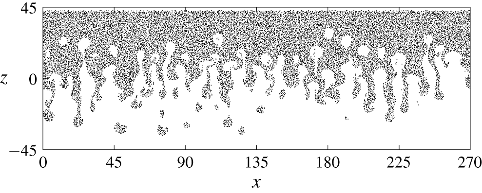
Particles at the central slice in the  $y$-direction at
 $t=63.71$ in the case of multi-mode simulation. Point markers are used to represent the positions of the particles in
 $L_{y}/2-0.1\unicode[STIX]{x1D6FF}y\leqslant y\leqslant L_{y}/2$, in which
 $L_{y}$ is the domain size in the
 $y$-direction and
 $\unicode[STIX]{x1D6FF}y$ is the grid size in the
 $y$-direction.

The origin of the horizontal coordinate is defined at the centroid of the horizontal plane (i.e.,  $-L_{x}/2\leqslant x\leqslant L_{x}/2$ and
 $-L_{y}/2\leqslant y\leqslant L_{y}/2$). As shown in figure 1(c), an initial single-mode perturbation (
 $\unicode[STIX]{x1D702}$) at the interface between the particle-laden layer and the clear fluid is given by
 $$\begin{eqnarray}\unicode[STIX]{x1D702}=\left\{\begin{array}{@{}ll@{}}1.30\left(1+\cos \left({\displaystyle \frac{2\unicode[STIX]{x03C0}r}{\unicode[STIX]{x1D706}}}\right)\right),\quad & \text{if }r<{\displaystyle \frac{\unicode[STIX]{x1D706}}{2}},\\ 0,\quad & \text{otherwise},\end{array}\right.\end{eqnarray}$$
where  $r=\sqrt{x^{2}+y^{2}}$. The bottom interface of the particle-laden layer is located at the middle of the background temperature gradient, where the perturbation given by (2.16) is also applied to the temperature field. The value of the length of perturbation
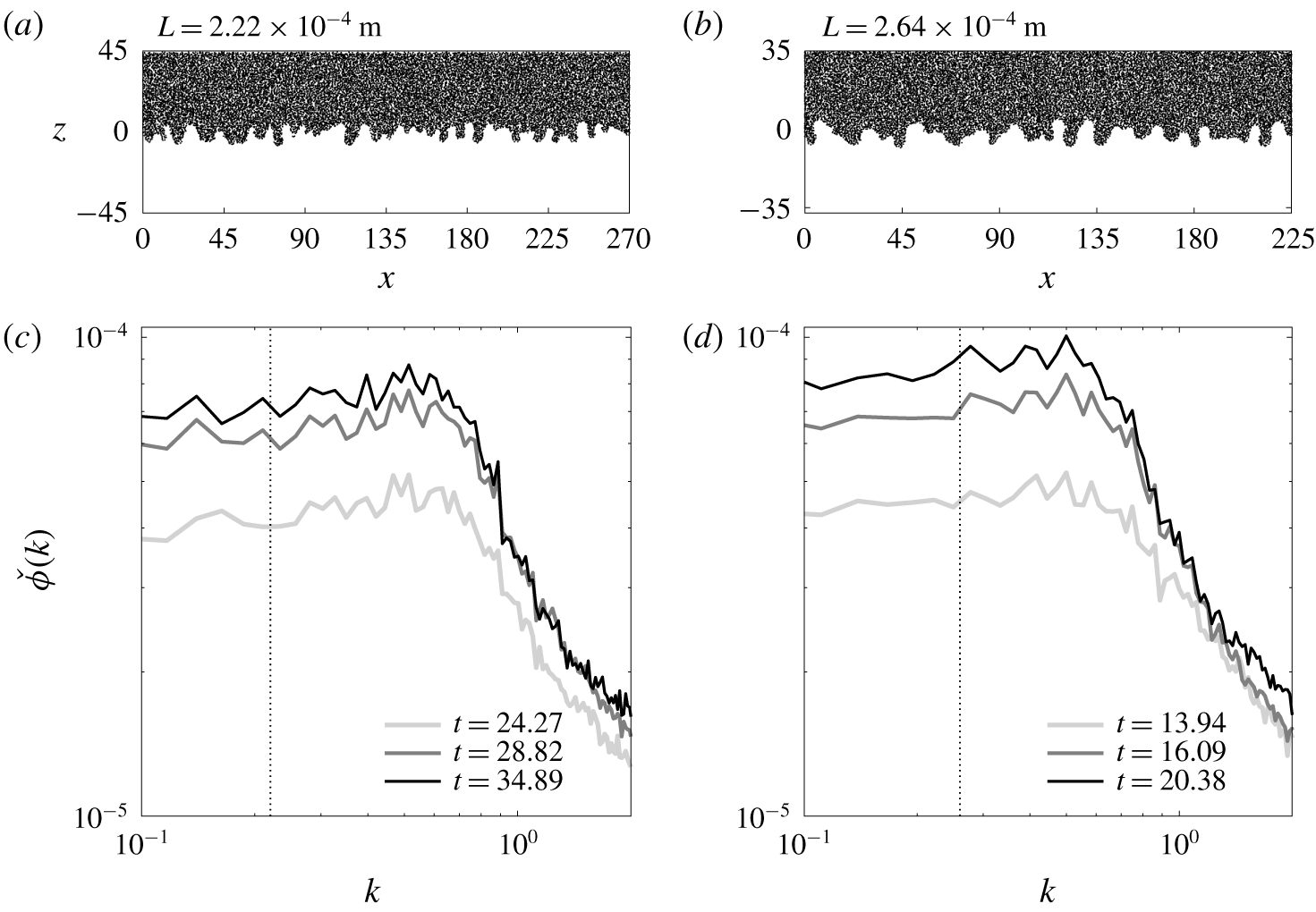
 $\unicode[STIX]{x1D706}=12$ is chosen based on the most energetic mode in a multi-mode simulation (see appendix B). A representative snapshot of particles in the multi-mode case is presented in figure 2, and its simulation set-up is summarized in appendix B. Figure 2 shows that fingers are fairly symmetric about the vertical centre (
 $z=0$), which indicates that the sedimentation pattern is double-diffusive convection, rather than the settling-driven RTI according to Yu et al. (Reference Yu, Hsu and Balachandar2014) and Burns & Meiburg (Reference Burns and Meiburg2015). However, due to the initially sharp interface of the particle-laden layer, even when
 $w_{s}\approx 0$, RTI may occur in the case of a low background temperature gradient. If this were the case, as shown in appendix B, the dominant wavenumber would be less than half of the present dominant mode. Therefore, one can argue that the sedimentation pattern in the present cases is dominated by the double-diffusive convection. In the rest of the paper, we focus on individual plumes by imposing a single-mode perturbation at the particle-laden interface. In fact, because the randomness and discreteness of particle distribution always pose infinitesimal perturbations, a pure single-mode plume is impossible to generate in the domain in the particle-laden case. However, the perturbation given by (2.16) allows for a single plume that develops faster than any others during the simulation, thus enabling a detailed investigation of a single plume without interference from neighbouring plumes.
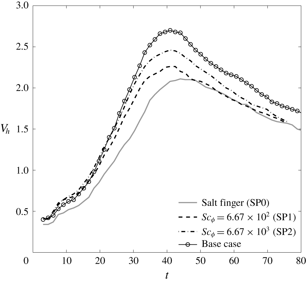
In addition to those EL cases mentioned above, three cases of single-phase (SP) simulation are conducted. The first is the simulation of a salt finger in the same simulation set-up, and the other two adopt the scalar-limit approximation for the simulation of sediment transport for the case of  $w_{s}=3.33\times 10^{-2}$ but with different diffusivities. The SP simulations are conducted to examine the differences between the particles and the ‘dissolved’ scalar field. The simulation set-up for each case is given in table 1. Of the present cases, EL simulation using
 $w_{s}=3.33\times 10^{-2}$ serves as the base case, the results of which are used for the discussion in the following two sections.
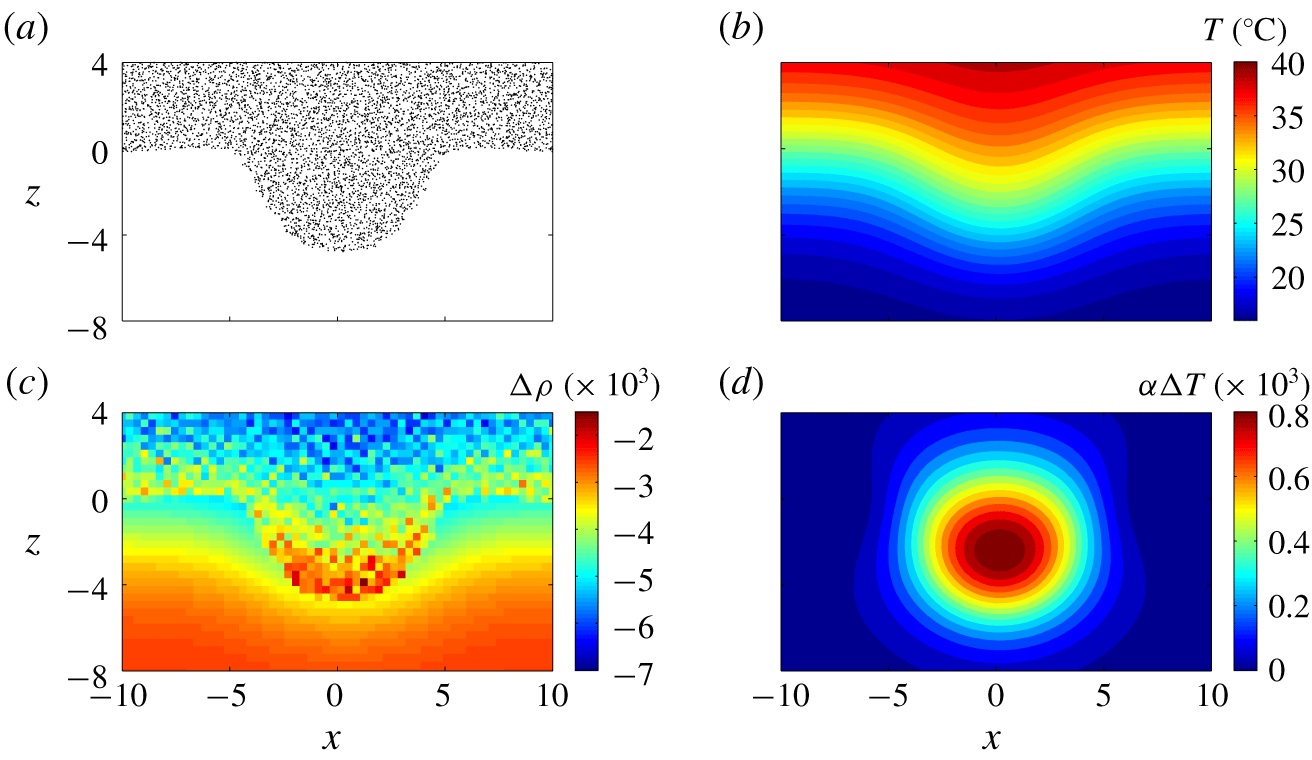
Representative snapshots of particles (a), temperature  $T$ (b), total density anomaly
 $\unicode[STIX]{x0394}\unicode[STIX]{x1D70C}$ (c), and the density anomaly due to temperature perturbation
 $\unicode[STIX]{x1D6FC}\unicode[STIX]{x0394}T$ (d) at the particle-laden interface at the central slice in the
 $y$-direction in the base at
 $t=4.55$, showing the growth of the initial perturbation of the particle-laden interface during the early stage. In panel (a), point markers are used to represent the positions of the particles located in
 $L_{y}/2-\unicode[STIX]{x1D6FF}y\leqslant y\leqslant L_{y}/2$, in which
 $L_{y}$ is the domain size in the
 $y$-direction and
 $\unicode[STIX]{x1D6FF}y$ is the grid size in the
 $y$-direction.

3 Evolution of the particle-laden finger
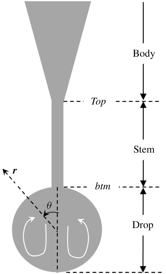
The formation and evolution of a double-diffusive particle-laden finger and the resulting drop can be described in four stages as follows. In this section, we focus our discussion on the base case (d05C084; see table 1). Deviations of the other cases from the base case are presented in §§ 5–7.
3.1 Stage 1: double-diffusion finger
Figure 3 shows representative snapshots of the particle distribution, temperature, total density anomaly, and density anomaly  $\unicode[STIX]{x1D6FC}\unicode[STIX]{x0394}T$ due to perturbed temperature
 $\unicode[STIX]{x0394}T=T-T_{r}$ at the beginning time point, to demonstrate the mechanism responsible for the growth of the initial perturbation at the particle-laden interface. Here, the total density anomaly
 $\unicode[STIX]{x0394}\unicode[STIX]{x1D70C}$ is obtained with
 $$\begin{eqnarray}\unicode[STIX]{x0394}\unicode[STIX]{x1D70C}=\unicode[STIX]{x1D6FE}\unicode[STIX]{x1D719}-\unicode[STIX]{x1D6FC}\unicode[STIX]{x0394}T,\end{eqnarray}$$
where  $\unicode[STIX]{x1D719}$ is obtained by summing the volume fraction of all particles in a grid cell. As shown in figure 3(a,b), the initial perturbation of the particle-laden interface results in a perturbation in the background temperature. Here, temperature acts as an agent that diffuses much faster than particles, and the density anomaly (
 $\unicode[STIX]{x0394}T$) peaks at the body of the perturbed particle-laden plume but decreases toward the tip of the plume, as shown in figure 3(d). As shown in figure 3(c), this results in an increase in the bulk density at the tip of the plume, which becomes heavier than surrounding fluid and leads to instability of the interface. The mechanism by which the particle-laden plume becomes heavier than the surrounding fluid due to relatively rapid thermal exchange was discussed by Parsons & Garcia (Reference Parsons and Garcia2000) in the context of double-diffusive sedimentation and is analogous to the mechanism that causes double-diffusive salt fingers in oceans.
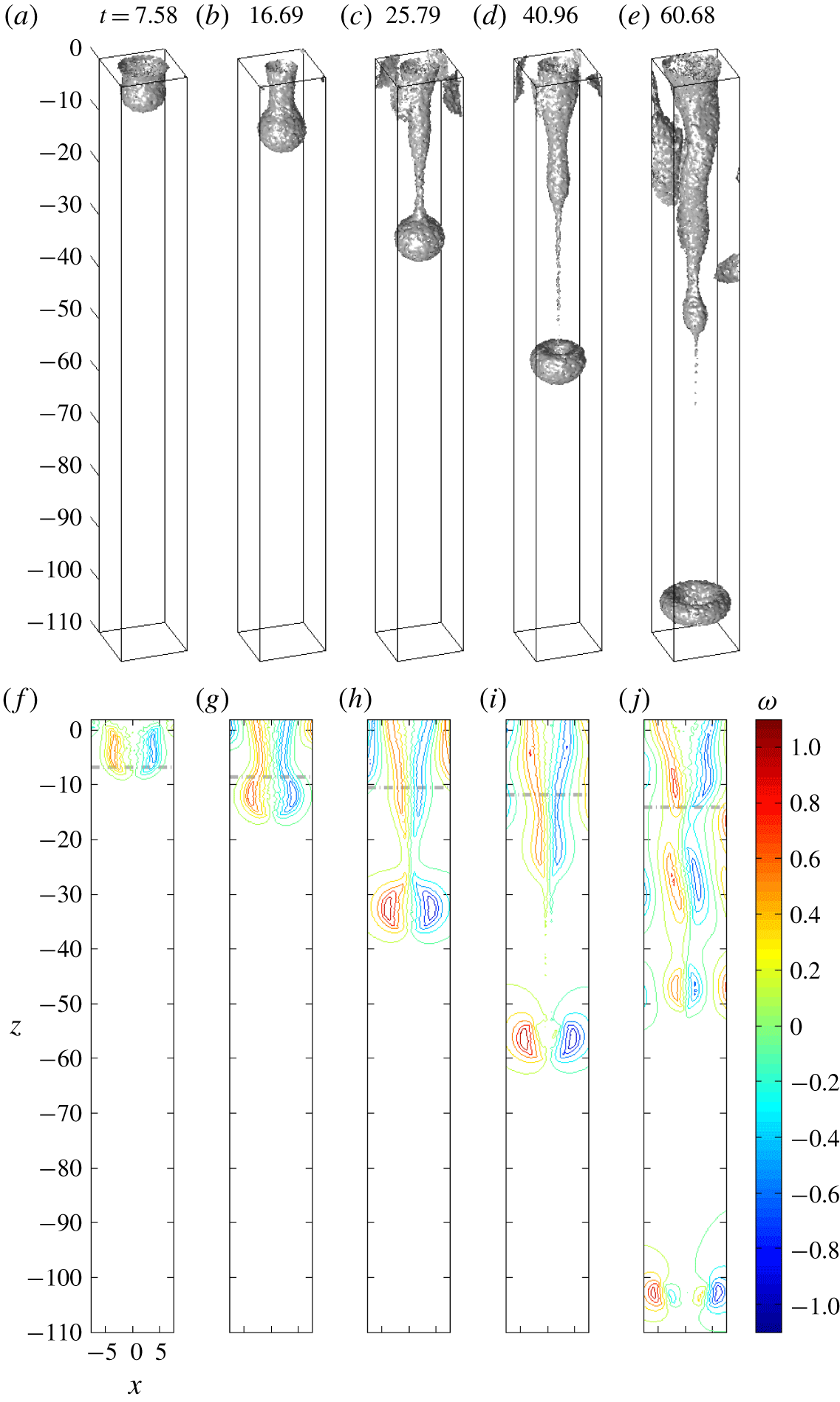
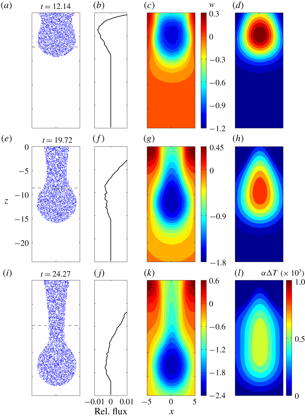
Figure 4 presents a series of snapshots of the isosurfaces of the particle concentration  $\unicode[STIX]{x1D719}/\unicode[STIX]{x1D719}_{0}=0.5$ and the associated vorticity fields at representative time points. Following the instability mentioned previously, the perturbation grows and becomes a descending plume, also known as a finger, (see figure 4a,b). As shown in figure 4(f,g), associated with the onset of the plume are the strong vortices (i.e., the vortex ring) at the interface of the particle-laden layer. As indicated by the grey dash-dotted lines in figure 4(f,g) that mark the lower boundary of the region of the temperature gradient, the movement of the plume during this stage is mostly confined within the region of the temperature gradient. Figure 5 shows a series of representative snapshots of the particle-laden plume, the mass flux relative to movement of the plume head, the associated vertical velocity and the density anomaly
 $\unicode[STIX]{x1D6FC}\unicode[STIX]{x0394}T$ due to perturbed temperature
 $\unicode[STIX]{x0394}T$. A characteristic of this stage is the coincidence of the maximum vertical speed and the temperature perturbation (i.e.,
 $\unicode[STIX]{x0394}T\sim \int (\unicode[STIX]{x2202}T_{r}/\unicode[STIX]{x2202}z)w\,\text{d}t$; see figure 5c,d). Figure 5(a) shows that the plume head with a bulbous shape is just beginning to form and, as shown in figure 5(c), the velocity maximum is located slightly above the vertical centre of the bulbous head. At this stage the movement of the plume is slow, and the negative vertical velocity at the top of the bulbous head leads to a significant inflow mass flux into the head region (see figure 5b).
Representative snapshots of isosurfaces of  $\unicode[STIX]{x1D719}/\unicode[STIX]{x1D719}_{0}=0.5$ (a–e) and the corresponding vorticity at the central slice in the
 $y$-direction. Grey dashed lines in (f–j) indicate the locations where
 $T_{r}=T_{r,low}+0.1(T_{r,up}-T_{r,low})$, which are used to indicate the locations of the plume relative to the gradient of the background temperature.

Snapshots of the particle-laden finger (a,e,i), vertical velocity (c,g,k), density anomaly due to temperature perturbation (d,h,l) at the central slice in the  $y$-direction at representative time steps and the corresponding mass flux relative to the movement of the plume head (b,f,j). In the particle plots, point markers are used to represent the positions of the particles located in
 $L_{y}/2-\unicode[STIX]{x1D6FF}y\leqslant y\leqslant L_{y}/2$, in which
 $L_{y}$ is the domain size in the
 $y$-direction and
 $\unicode[STIX]{x1D6FF}y$ is the grid size in the
 $y$-direction.

After the head of the descending plume leaves the region of the sharp temperature gradient, as shown in figure 5(g,h), the region of maximum vertical speed begins to deviate from the region of maximum  $\unicode[STIX]{x0394}T$. As the descending speed of the bulbous head increases, as shown in figure 5(f), the inflow mass flux becomes weaker compared with figure 5(b). The evolution progresses and, as shown in figure 5(i), when the bulbous head completely leaves the region of the temperature gradient, it is associated with a descending speed much greater than that in the thermal-controlled double-diffusive region due to the decreasing temperature anomaly. As shown in figure 5(l), the maximum temperature anomaly is retained near the lower boundary of the temperature gradient, which makes buoyant forcing significantly weaker than that in the head region. Moreover, because of the head’s high descending speed, the inflow mass flux from the parent plume vanishes (see figure 5i); the bulbous head then begins to detach from its parent plume and forms a drop, which marks the end of the double-diffusion stage.
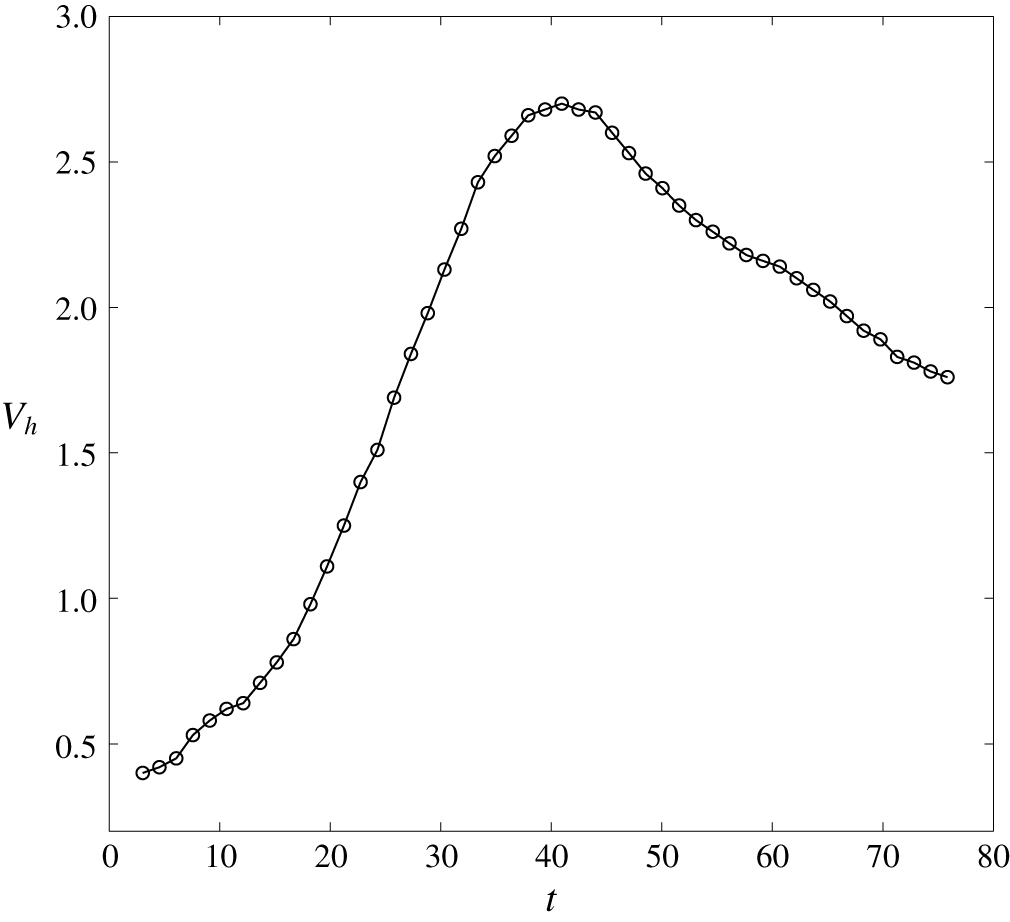
Time history of the descending speed  $V_{h}$ of the plume head in the base case (
 $w_{s}=3.33\times 10^{-2}$).

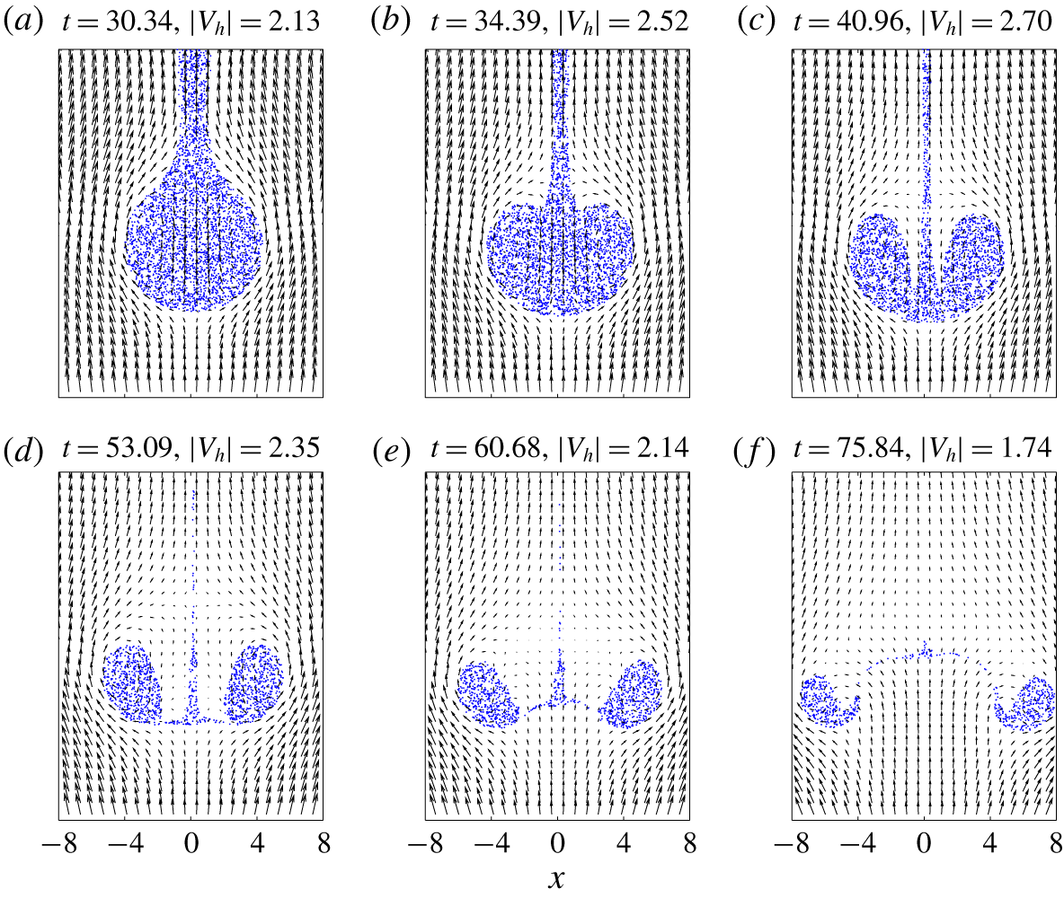
Snapshots of the particle-laden drop superimposed with the velocity field on the reference frame moving with the drop during the pinch-off process. Point markers are used to represent the positions of the particles located in  $L_{y}/2-\unicode[STIX]{x1D6FF}y\leqslant y\leqslant L_{y}/2$, in which
 $L_{y}$ is the domain size in the
 $y$-direction and
 $\unicode[STIX]{x1D6FF}y$ is the grid size in the
 $y$-direction.

3.2 Stage 2: transition to the spheroidal drop and entrainment
When the head of the plume leaves the region of the temperature gradient and arrives at the region of uniform temperature, the temperature perturbation within the drop decreases continuously, causing the total density anomaly ( $\unicode[STIX]{x0394}\unicode[STIX]{x1D70C}$) to increase during the drop’s descent. At this moment, a spheroidal drop can be clearly seen (see figure 4c) connected to the plume’s body via a thinning stem. The drop enters a significant acceleration phase (see
 $20<t<30$ in figure 6). Also, as shown by the vorticity contours in figure 4(h), the separation of the vorticity within the head from the body of the plume indicates the onset of a pinch-off of the vortex ring, as discussed in the context of jet flows (e.g., Zhao, Frankel & Mongeau Reference Zhao, Frankel and Mongeau2000; Wang et al. Reference Wang, Law, Adams and Fringer2009). The thinning stem eventually breaks (see figure 4d), and the spheroidal drop becomes an isolated ring torus (see figure 4(d,i) for the vorticity field) that freely descends in the water column.
As shown in figure 7(a), the initial shape of the drop resembles a drop of liquid in the air, whose lower half is a hemisphere and whose upper half is somewhat elongated. There seems to be a little wake behind the drop in the present case. A wake region may or may not exist, depending on the drop Reynolds number,  $Re_{d}=V_{h}D/\unicode[STIX]{x1D708}$, in which
 $D$ is the diameter of the drop’s frontal area projected onto the incoming flow. Here,
 $D$s are estimated by measuring the greatest distance between particles sampled in the region near the central slice in the
 $y$-direction (i.e.,
 $L_{y}/2-2\unicode[STIX]{x1D6FF}y\leqslant y\leqslant L_{y}/2+2\unicode[STIX]{x1D6FF}y$). Due to the axisymmetric feature of the drop, this provides a satisfactory estimation for
 $D$. Flow in the wake region can result in an outflow mass flux from the drop (i.e., detrainment of particles from the head to the stem). However, as shown in figure 5(j), the increasing relative mass flux with the depth (negative
 $z$-direction) in the upper region, and the decreasing relative mass flux with the depth in the lower region of the drop, result in gradual vertical compression of the drop. This is reminiscent of Hill’s vortex, subject to an oblate perturbation (Pozrikidis Reference Pozrikidis1986). As a result, the particle moves away from the wake at the rear of the drop, as shown in figure 7(b). As this occurs, the detrainment of particles in the drop ceases, and the presence of the thinning stem retains a weak particle inflow flux to the drop.
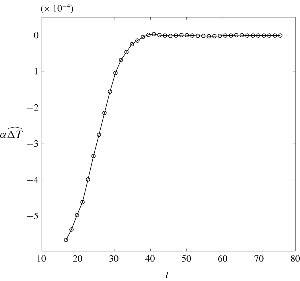
During the later stage following the disappearance of the particle-containing wake, the ambient flow begins to be entrained into the drop, as shown in figure 7(b,c). This coincides with the thinning of the stem. As shown in figure 6, the drop attains its terminal speed at  $t=40.96$ (see figure 7c for a snapshot of the particles), which is the time at which the temperature perturbation within the drop vanishes completely. This can be seen from the time history of the volume-averaged density anomaly due to temperature perturbation within the drop in figure 8. Although the entrainment that begins around
 $t=34$ somewhat suppresses the drop’s acceleration (see figure 6), the drop attains its terminal speed only because the temperature perturbation disappears, which causes the total buoyant forcing to attain its maximum. As shown in figure 7(d), when the drop detaches from the stem, its shape becomes an oblate spheroid due to entrainment of the ambient fluid; this phenomenon is consistent with the nonlinear analysis for a perturbed Hill’s vortex in Pozrikidis (Reference Pozrikidis1986).
Time history of the volume-averaged density anomaly due to temperature perturbation within the drop in the base case shows that the disappearance of the volume-averaged temperature perturbation,  $\unicode[STIX]{x1D6FC}\widetilde{\unicode[STIX]{x0394}T}$ (
 $\unicode[STIX]{x0394}T=T-T_{r}$), corresponds to a peak
 $V_{h}$ in figure 6.

3.3 Stage 3: buoyant vortex ring
As shown in figure 7(d), upon its detachment from the stem, the particle-laden drop differs from the typical torus-shaped vortex ring in the presence of a thin bottom boundary formed by suspended particles the frontal region. After the stem disappears, the lack of mass supplied from the stem makes this particle-containing bottom boundary thinner and diluted, and its descending motion becomes slower relative to that of the ring (i.e., the vortex pair), as shown in figure 7(e,f). According to Turner (Reference Turner1957), under the similarity assumption, the motion of a buoyant vortex ring in a uniform surrounding follows  $V_{h}a\sim \unicode[STIX]{x1D6E4}$, in which
 $\unicode[STIX]{x1D6E4}$ is the circulation and
 $a=D/2$ is the radius of the ring. In our simulation, viscous dissipation causes little decrease in
 $\unicode[STIX]{x1D6E4}$ during the stage after pinch-off, and
 $V_{h}a$ does not significantly vary over time, as discussed in § 4.
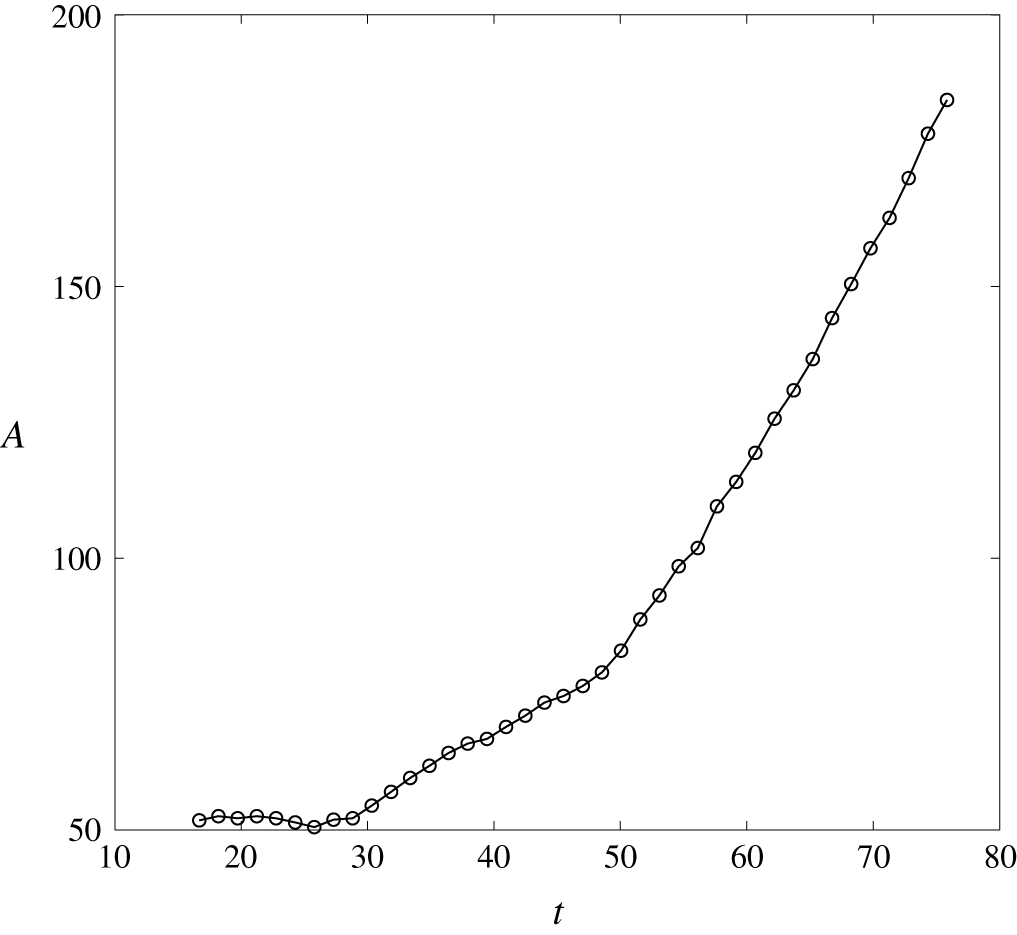
Time history of the projection area to the incoming flow,  $A=1/4\unicode[STIX]{x03C0}D^{2}$, of the drop in the base case.

Figure 9 presents the time history of the projection area of the drop,  $A=1/4\unicode[STIX]{x03C0}D^{2}$, to the incoming flow in the base case. One may compare figure 9 with the theory of buoyant vortex rings (Turner Reference Turner1957). That is, for a vortex ring with circulation
 $\unicode[STIX]{x1D6E4}$ and density
 $\unicode[STIX]{x1D70C}$, the impulse
 $I$ can be obtained with the relationship (Lamb Reference Lamb1932),
 $$\begin{eqnarray}I=\unicode[STIX]{x1D70C}A\unicode[STIX]{x1D6E4}.\end{eqnarray}$$
With the buoyant force acting on the ring (Turner Reference Turner1957)
 $$\begin{eqnarray}{\displaystyle \frac{\text{d}I}{\text{d}t}}=g\unicode[STIX]{x1D6FA}_{rg}\unicode[STIX]{x0394}\unicode[STIX]{x1D70C},\end{eqnarray}$$
where  $\unicode[STIX]{x1D6FA}_{rg}$ is the volume of the ring. Now, a combination of (3.2) and (3.3) shows that during the strong acceleration phase, when
 $20\leqslant t\leqslant 30$, the vanishing temperature perturbation within the drop (see figure 8) results in an internal change in both the bulk density
 $\unicode[STIX]{x1D70C}$ and the circulation
 $\unicode[STIX]{x1D6E4}$ in the drop but no significant change in
 $A$ (see figure 9). When the decrease in the temperature perturbation becomes slower (when
 $t>30$) (see figure 8) and when the total density anomaly
 $\unicode[STIX]{x0394}\unicode[STIX]{x1D70C}$ in (3.3) attains its maximum, the frontal area begins to increase. After
 $t=50$, which is the duration for which
 $\unicode[STIX]{x0394}\unicode[STIX]{x1D70C}$ retains its constant maximum value, and after complete detachment of the drop from the parent finger,
 $\unicode[STIX]{x1D6E4}$ becomes almost a constant, despite slight viscous dissipation, and figure 9 shows that
 $A$ increases almost linearly with time. In this condition, a combination of (3.2) and (3.3) gives
 $$\begin{eqnarray}{\displaystyle \frac{\text{d}I}{\text{d}t}}=\unicode[STIX]{x1D70C}\unicode[STIX]{x1D6E4}{\displaystyle \frac{\text{d}A}{\text{d}t}}=g\unicode[STIX]{x1D6FA}_{rg}\unicode[STIX]{x0394}\unicode[STIX]{x1D70C}.\end{eqnarray}$$
Equation (3.4) is a result of the assumption of constant circulation for the buoyant vortex ring in Turner (Reference Turner1957), which states that under a uniform background density, the frontal projection area  $A$ increases linearly with time, which is consistent with our simulation result in figure 9.
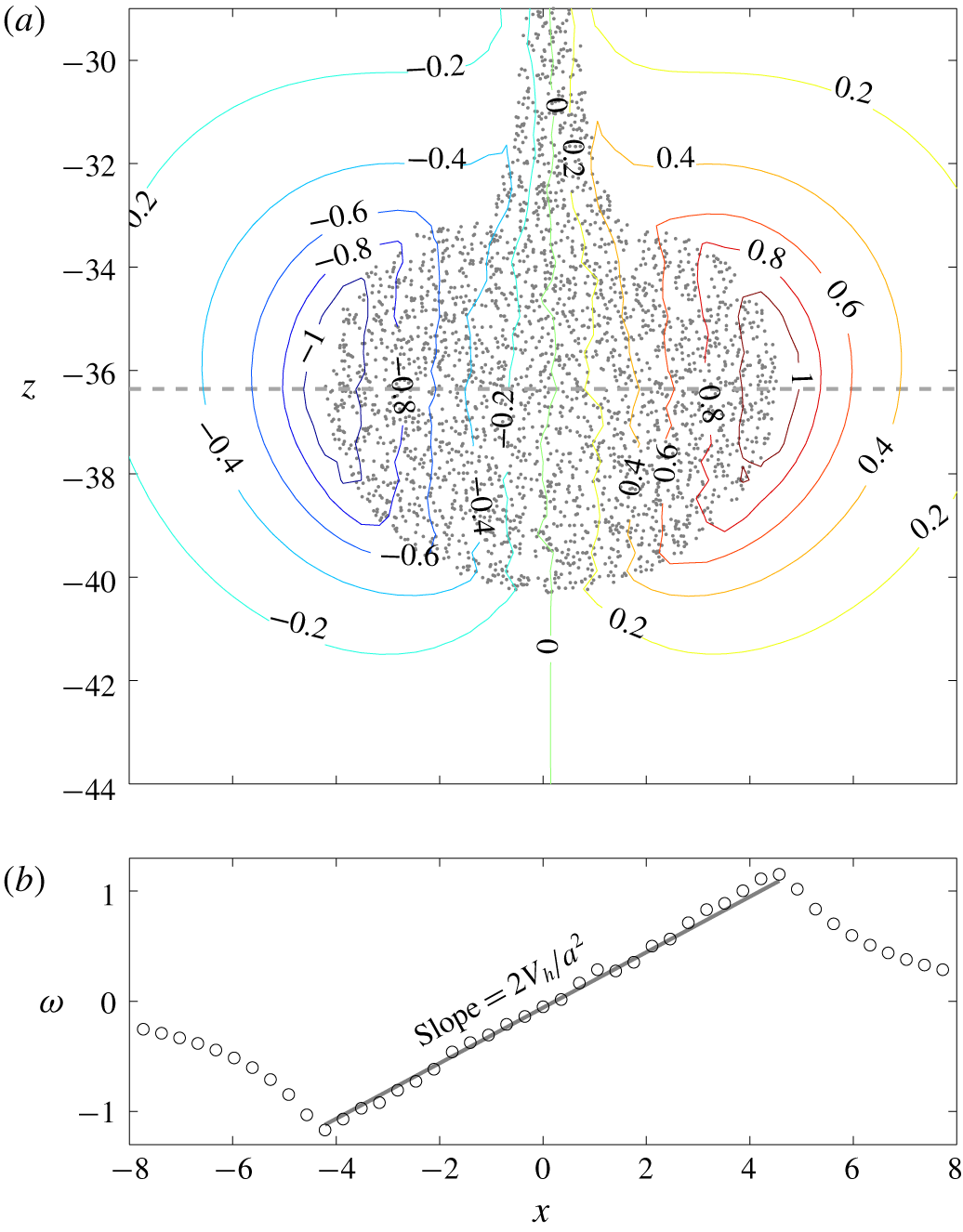
Particles at the central slice in the  $y$-direction superimposed with the corresponding vorticity field
 $\unicode[STIX]{x1D714}_{3}$ at
 $t=33.37$ (a) and a plot of
 $\unicode[STIX]{x1D714}$ as a function of
 $x$ along
 $y=-36.36$ (the grey dashed line in a) superimposed with a grey solid straight line with slope
 $=2V_{h}/a^{2}$ (b), showing the linear distribution of
 $\unicode[STIX]{x1D714}_{3}$ along the
 $x$-direction inside the drop. Point markers in (a) are used to represent the positions of the particles in
 $L_{y}/2-\unicode[STIX]{x1D6FF}y\leqslant y\leqslant L_{y}/2$, in which
 $L_{y}$ is the domain size in the
 $y$-direction and
 $\unicode[STIX]{x1D6FF}y$ is the grid size in the
 $y$-direction.

4 Spherical drop model
The dynamics of a particle-laden drop from its origin with the double-diffusive instability was given in detail in the previous section. Due to its slow motion and small size (i.e., low  $Re_{d}$), it is possible to construct a simple predictive model based on theoretical arguments which is given as follows in this section.
4.1 Model derivation
The vertical motion of the particle-laden drop in the present study can be expressed as
 $$\begin{eqnarray}\unicode[STIX]{x1D70C}\unicode[STIX]{x1D6FA}(1+c_{a}){\displaystyle \frac{\text{d}V_{h}}{\text{d}t}}=B-\unicode[STIX]{x1D70C}_{0}C_{d}AV_{h}^{2}+q_{in},\end{eqnarray}$$
where  $\unicode[STIX]{x1D6FA}$ is the volume of the drop,
 $c_{a}$ is the added mass coefficient,
 $B$ represents the buoyant force combining the temperature and particle-laden effects,
 $C_{d}$ is the drag coefficient and
 $q_{in}$ is the momentum flux via the stem before pinch-off. In our cases, the momentum flux
 $q_{in}$ is much lower than the other terms as long as an apparent bulbous shape forms at the plume head. Moreover, the acceleration term is much lower than either the buoyancy or the drag. That is, the descending drop is in a state of quasi-equilibrium for which the drag soon attains near equilibrium with the body force. Therefore, one can have
 $$\begin{eqnarray}\displaystyle C_{d} & {\approx} & \displaystyle C_{d,eq}\;,\nonumber\\ \displaystyle & = & \displaystyle {\displaystyle \frac{\unicode[STIX]{x1D6FA}\widehat{b}}{\frac{1}{2}\unicode[STIX]{x1D70C}_{0}AV_{h}^{2}}},\end{eqnarray}$$
where  $C_{d,eq}$ is the drag coefficient in the state of equilibrium and
 $\widehat{b}$ is the volume-averaged body force of the drop. The falling velocity does not attain its terminal (steady) value immediately, mainly because the buoyant force varies over time as the temperature perturbation decreases continuously throughout the second stage of evolution (see § 3.2), resulting in the change in
 $V_{h}$.
It is important to examine how the drag coefficient obtained from (4.2) in our simulation compares with the theoretical model of the spherical drop. The solution can be obtained by solving the creeping flow equations on a spherical coordinate system  $(r,\unicode[STIX]{x1D703},\unicode[STIX]{x1D713})$ with proper boundary conditions. Although the no-penetration and far-field conditions are consistent with conventional creeping flow solution around a solid sphere, the boundary condition for the tangential velocity (
 $u_{\unicode[STIX]{x1D703}}$) on the drop’s surface in this case differs from the no-slip condition. This is similar to the analysis in early studies (Hadamard Reference Hadamard1911; Rybczynski Reference Rybczynski1911; Boussinesq Reference Boussinesq1913) on viscous drag of fluid spheres (e.g., bubbles). However, because these studies focus on the interfacial momentum jump or continuity for the boundary condition, none of them are found to be relevant to the present case. Here, the appropriate boundary condition can be obtained from the vorticity field, which is caused by baroclinic forcing (
 $\left(\unicode[STIX]{x1D735}\unicode[STIX]{x1D70C}\times \unicode[STIX]{x1D735}p\right)/\unicode[STIX]{x1D70C}^{2}$) on the drop’s surface. Therefore, for the vorticity field
 $\unicode[STIX]{x1D714}_{\unicode[STIX]{x1D713}}$, one can simply have
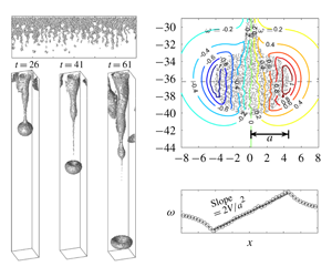
 $\unicode[STIX]{x1D714}_{\unicode[STIX]{x1D713}}\propto -D\sin \unicode[STIX]{x1D703}$ along the drop’s surface. This is demonstrated in figure 10(a), in which we plot the vorticity field superimposed with the particles for a particle-laden drop at
 $t=34.89$. As shown in figure 10(a), a linear distribution of the vorticity with respect to the
 $x$-axis within the drop can be found that corresponds to
 $D\sin \unicode[STIX]{x1D703}$ in the spherical coordinate. Therefore, the required boundary condition for solution of the creeping flow over this spherical drop can be obtained as
 $\unicode[STIX]{x1D714}=-E\sin \unicode[STIX]{x1D703}$, in which
 $E$ is a constant in space. Now, as a common practice of the creeping flow solution, on the reference following the drop motion, the theoretical result can be obtained by solving
 $$\begin{eqnarray}\displaystyle & \displaystyle \unicode[STIX]{x1D735}p=\unicode[STIX]{x1D707}\unicode[STIX]{x1D6FB}^{2}\boldsymbol{u}, & \displaystyle\end{eqnarray}$$
 $$\begin{eqnarray}\displaystyle & \displaystyle \unicode[STIX]{x1D735}\boldsymbol{\cdot }\boldsymbol{u}=0 & \displaystyle\end{eqnarray}$$
on the spherical coordinate system with zero  $u_{\unicode[STIX]{x1D719}}$. The boundary conditions are
 $$\begin{eqnarray}\displaystyle & \displaystyle \boldsymbol{u}=V_{h}\boldsymbol{e}_{z}\quad \text{as }|\boldsymbol{r}|\rightarrow \infty , & \displaystyle\end{eqnarray}$$
 $$\begin{eqnarray}\displaystyle & \displaystyle u_{r}=0\quad \text{on }|\boldsymbol{r}|=a, & \displaystyle\end{eqnarray}$$
 $$\begin{eqnarray}\displaystyle & \displaystyle \unicode[STIX]{x1D714}=-E\sin \unicode[STIX]{x1D703}\quad \text{on }|\boldsymbol{r}|=a, & \displaystyle\end{eqnarray}$$
where  $\boldsymbol{e}_{z}$ is the unit direction in the
 $z$-direction. Solution of (4.3) to (4.7) gives the velocity field
 $$\begin{eqnarray}\displaystyle & \displaystyle u_{r}=V_{h}\cos \unicode[STIX]{x1D703}\left[1-J{\displaystyle \frac{a}{r}}-(1-J){\displaystyle \frac{a^{3}}{r^{3}}}\right], & \displaystyle\end{eqnarray}$$
 $$\begin{eqnarray}\displaystyle & \displaystyle u_{\unicode[STIX]{x1D703}}=-V_{h}\sin \unicode[STIX]{x1D703}\left[1-{\displaystyle \frac{J}{2}}{\displaystyle \frac{a}{r}}+{\displaystyle \frac{1}{2}}(1-J){\displaystyle \frac{a^{3}}{r^{3}}}\right], & \displaystyle\end{eqnarray}$$
where
 $$\begin{eqnarray}J={\displaystyle \frac{Ea}{V_{h}}}\end{eqnarray}$$
and  $a=D/2$ is the radius. By integrating the stress in the streamwise direction along the surface to obtain the drag force, the theoretical drag coefficient can be obtained with
 $$\begin{eqnarray}C_{d,theo}={\displaystyle \frac{16J}{Re_{d}}},\end{eqnarray}$$
where  $Re_{d}=V_{h}D/\unicode[STIX]{x1D708}$ is the drop Reynolds number. In fact, as (4.3) is equivalent to
 $\unicode[STIX]{x1D6FB}^{2}\unicode[STIX]{x1D714}=0$, equation (4.7) (along with a far-field condition) can be a more general boundary condition for creeping flow solution given that the sources of the vorticity are generated at the boundary from various types of forcing, such as viscosity and the baroclinic effect. For example,
 $J=3/2$ corresponds to the no-slip boundary condition
 $u_{\unicode[STIX]{x1D703}}=0$ on
 $|\boldsymbol{r}|=a$, and
 $J=0$ (i.e.,
 $\unicode[STIX]{x1D74E}=0$) corresponds to a spherical vortex ring in irrotational flow.
Next, we must find the value of  $J$ for our case. It can be seen from figure 10 that
 $\unicode[STIX]{x1D714}$ linearly depends on
 $x$ within the drop, such that it can be expressed as
 $$\begin{eqnarray}\displaystyle \unicode[STIX]{x1D714} & = & \displaystyle -E\sin \unicode[STIX]{x1D703}{\displaystyle \frac{r}{a}}\nonumber\\ \displaystyle & = & \displaystyle {\displaystyle \frac{E}{a}}x\nonumber\\ \displaystyle & = & \displaystyle {\displaystyle \frac{V_{h}J}{a^{2}}}x,\end{eqnarray}$$
where the third identity is obtained by substituting (4.10) into the second identity. In fact, while  $E/a$ is the slope for the linear relationship between
 $\unicode[STIX]{x1D714}$ and
 $x$ in the drop,
 $J$ represents a non-dimensional slope obtained by normalizing
 $E/a$ by
 $V_{h}/a^{2}$. For Hill’s vortex, which is the spherical vortex ring in irrotational flow,
 $J=7.5$ (Hill Reference Hill1894; Moffatt & Moore Reference Moffatt and Moore1978). Here, as shown in figure 10(b), where we plot
 $\unicode[STIX]{x1D714}$ as a function of
 $x$ along
 $y=-36.36$ and compare it with a straight line with slope
 $=2V_{h}/a^{2}$,
 $J=2$ gives a good match with the present numerical results for the spherical ring of low
 $Re$. The final form of the drag coefficient is thus obtained by substituting
 $J=2$ into (4.11) to give
 $$\begin{eqnarray}C_{d,theo}={\displaystyle \frac{32}{Re_{d}}}.\end{eqnarray}$$
At this point, it is worthwhile to mention that although it is possible to obtain a higher-order solution (in terms of  $Re_{d}$) based on the Oseen equations, the present boundary condition, equation (4.7), does not allow us to construct the special solution for the flow field at higher order. However, as shown in appendix C, the drag coefficient (4.13) obtained here is consistent with that obtained from the Oseen equations up to first order (
 $O(Re_{d})$).
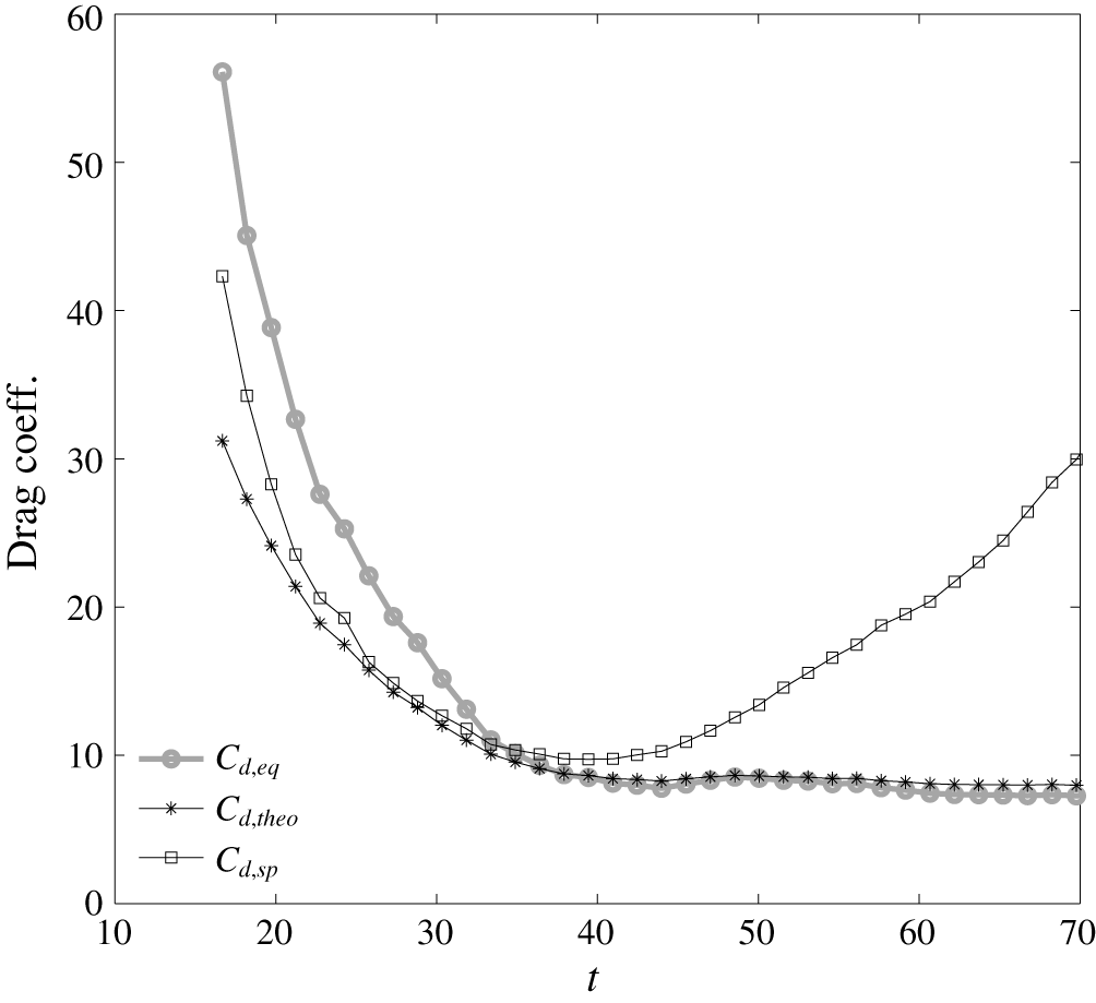
Time histories of various drag coefficients in the base case ( $w_{s}=3.33\times 10^{-2}$).

4.2 Comparison with numerical results
Figure 11 compares time histories of  $C_{d,eq}$ and
 $C_{d,theo}$ after an apparent drop shape is seen (i.e.,
 $t>16$). An underestimation by the theoretical model before
 $t=32$ is shown. It should be noted that the present predictive model for the drop’s speed is derived for an isolated, spherical drop. Therefore, as discussed in what follows, good model predictability during the early stage before the drop’s detachment from the parent finger is not anticipated. A major contribution to the discrepancy in the theoretical prediction (
 $C_{d,theo}$) is the deviation of the drop’s actual shape from a sphere. To show this, we define an effective drag coefficient for a spherical drop by replacing an effective spherical volume
 $\unicode[STIX]{x1D6FA}_{sp}=4/3\unicode[STIX]{x03C0}a^{3}$ with the actual drop volume
 $\unicode[STIX]{x1D6FA}$ (from computational results) in (4.2) to obtain an effective spherical drag coefficient
 $$\begin{eqnarray}C_{d,sp}={\displaystyle \frac{\unicode[STIX]{x1D6FA}_{sp}\widehat{b}}{\frac{1}{2}\unicode[STIX]{x1D70C}AV_{h}^{2}}}.\end{eqnarray}$$
As shown in figure 11, the discrepancy in the theoretical prediction can be reduced considerably when compared with  $C_{d,sp}$. Another contribution to the difference between the theoretical prediction and the actual values of the drag coefficient during the early development stage is that the bulbous head remains connected to the plume’s body (i.e., parent finger). This results in an inflow vorticity flux to the head, which makes the actual value of
 $J$ greater than 2. The resulting underestimation by the theoretical prediction using
 $J=2$ can be clearly seen during the very early stage (i.e.,
 $t<25$) in figure 11. Because the connection between the head and the body is weaker and pinch-off occurs,
 $J$ is close to 2 after
 $t=34$ and the shape of the drop is more spherical. At this stage, figure 11 shows a fairly good agreement between the theoretical prediction
 $C_{d,theo}$ and
 $C_{d,eq}$. However, although
 $C_{d,theo}$ and
 $C_{d,eq}$ are close to each other,
 $C_{d,sp}$ begins to deviate from the two at
 $t=34$, because entrainment occurs when
 $t>34$, and the drop is no longer spherical (see figure 7b,c). Once entrainment occurs, the drop behaves like the vortex ring with constant circulation, whose motion follows the similarity law (i.e.,
 $V_{h}a=\text{const.}$). As a result,
 $Re_{d}$ remains nearly a constant when
 $t>34$, and the drag coefficient does not vary significantly over time. That is, the similarity condition holds for the drop motion when entrainment occurs, and the resulting constant
 $Re_{d}$ leads to a fixed drag coefficient equivalent to the value just before entrainment occurs. As a result, fairly good agreement can still be found between
 $C_{d,theo}$ and
 $C_{d,eq}$, as shown by
 $t>34$ in figure 11, indicating a good predictability of
 $C_{d,theo}$ (4.13) during the stage after the drop reaches its terminal speed.
5 Effect of particle size
Because the present study focuses on particle-laden drops, the particle size can have an important influence on the flow dynamics. Here, we confine our discussion to fine particles whose motion is dominated by the flow (i.e.,  $w_{s}<1$). Cases with larger particles whose gravitational settling and inertia can be important are beyond the scope of this study. In this section, we examine effects of particle size by investigating four additional cases,
 $d_{0}=3$,
 $7$,
 $10$ and
 $14~\unicode[STIX]{x03BC}\text{m}$, that correspond to the non-dimensional settling speed
 $w_{s}=1.20\times 10^{-2}$,
 $6.67\times 10^{-2}$,
 $1.33\times 10^{-1}$ and
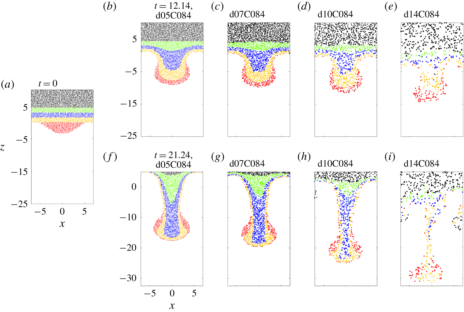
 $2.67\times 10^{-1}$, respectively, as summarized in table 1. In natural environments, these sizes correspond to fine silt and clay, which are the major components of suspended load in water bodies such as estuaries and rivers. Figure 12 shows snapshots of particles during the early stage in cases d05C084, d07C084, d10C084 and d14C084, in which we use four colours to track specific groups of particles. Typically, due to the associated greater gravitational settling, a larger particle size leads to a faster rate of vertical transport, which can be seen by comparison of the movement of the blue particles at the two time points (
 $t=12.14{-}21.24$) in cases d07C084 and d10C084. The resulting faster transport rate also leads to vertical stretching of the plume and to earlier detachment of the drop when particle sizes are larger. An interesting feature in figure 12 is the irregularities in particle distributions in case d14C084 relative to the other cases, which is due to the discreteness of the point-force distribution in cases with a low number density of particles (i.e., number of particles per unit volume). For a reference, the number density of particles in case d14C084 is approximately 22 times less than that of the base case (d05C84).
Snapshots of particles at the central slice in the  $y$-direction in cases of fine (
 $w_{s}=3.33\times 10^{-2}$, b and e), medium (
 $w_{s}=6.67\times 10^{-2}$, c and f), and large (
 $w_{s}=1.33\times 10^{-1}$, d and g) particle sizes at
 $t=12.14$ (b–e) and
 $21.24$ (f–i) during the early stages of evolution. Colours are used to track specific groups of particles. Panel (a) shows the corresponding initial snapshots in a case with fine size to show the initial distributions of various colours. Point markers are used to represent the relative size difference between the cases and positions of the particles located in
 $L_{y}/2-\unicode[STIX]{x1D6FF}y\leqslant y\leqslant L_{y}/2$, in which
 $L_{y}$ is the domain size in the
 $y$-direction, and
 $\unicode[STIX]{x1D6FF}y$ is the grid size in the
 $y$-direction.

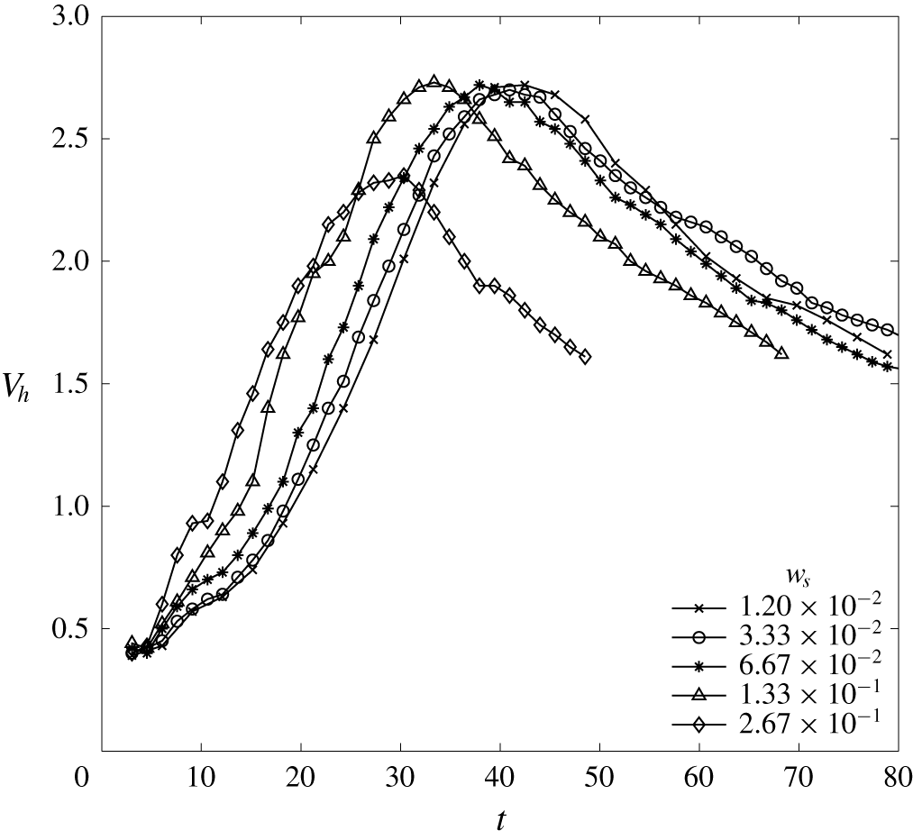
Figure 13 shows the time histories of  $V_{h}$ for various particle sizes which shows that the time histories of
 $V_{h}$ converge when the particle size becomes smaller, indicating that the particle size is less important in the drop dynamics when it is smaller, particularly when
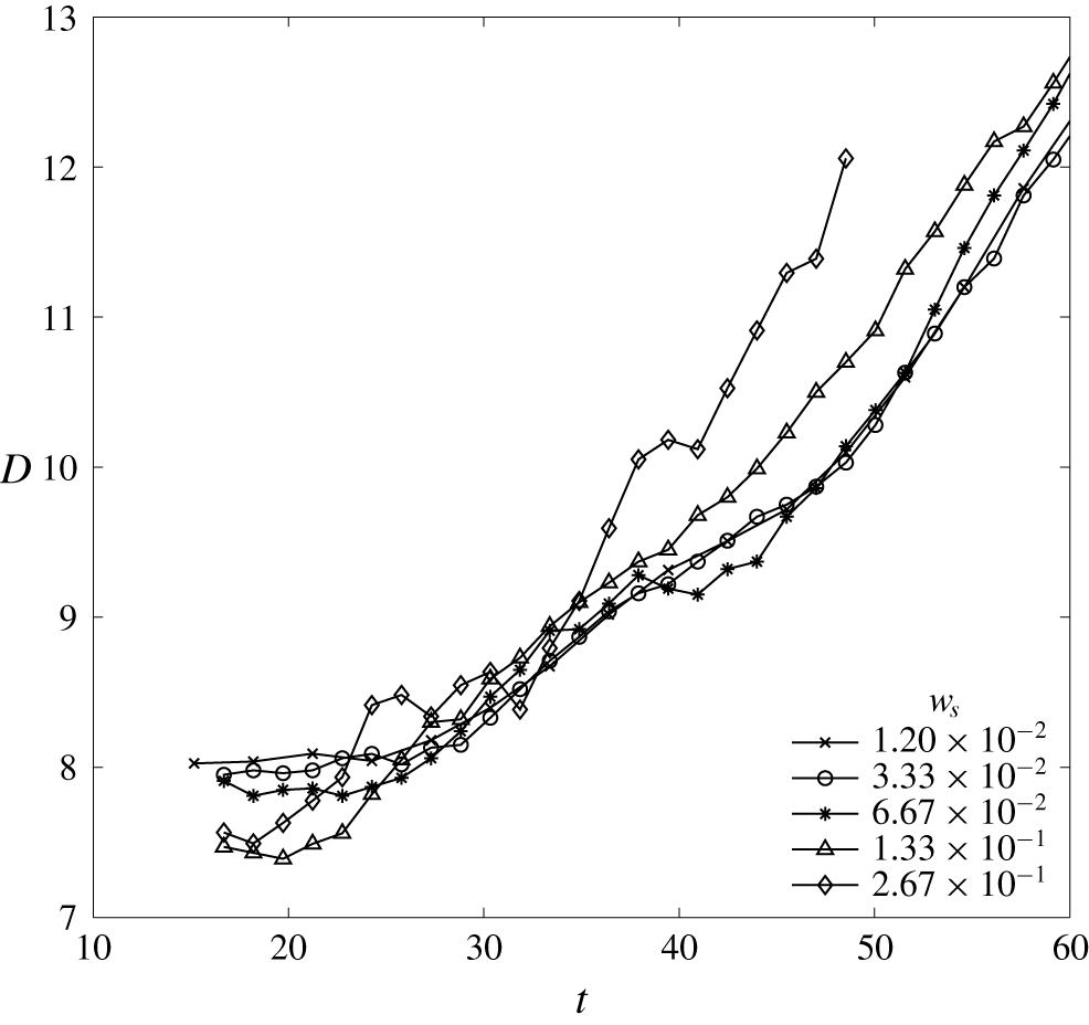
 $w_{s}<0.01$. Moreover, due to the equal bulk density and similar size (see figure 14) of the drop, the terminal speeds do not vary significantly among cases with various particle sizes, except for case d14C084. Case d14C084 has a slightly lower
 $V_{h}$ than the others mainly because of the greater projection area
 $A$ during the early development stage. This is demonstrated in figure 14, which shows the rapid growth of
 $D$ during the early stage (
 $t\approx 25$) in case d14C084 relative to the others. The rapid growth in
 $D$ in case d14C084 as shown in figure 14 results from the significantly faster vertical transport rate of particles that leads to a stronger oblate perturbation to the ring (see § 3.2). In fact, although
 $V_{h}$ in these cases ranges roughly from 0.5 to 3, one may expect that for larger particles with non-dimensional settling velocities only slightly less than unity (i.e., case d18C084), gravitational settling of individual particles can play a significant role in the dynamics during the early development stage of the drop.
Time histories of the descending speed  $V_{h}$ of the plume head in five cases with different particle sizes.

Time histories of the diameter  $D$ of the area projection to the horizontal plane of the plume head in five cases with various particle sizes. Here,
 $D$s are estimated by measuring the greatest distance between particles sampled in the region near the central slice in the
 $y$-direction,
 $L_{y}/2-2\unicode[STIX]{x1D6FF}y\leqslant y\leqslant L_{y}/2+2\unicode[STIX]{x1D6FF}y$, in which
 $L_{y}$ is the domain size in the
 $y$-direction and
 $\unicode[STIX]{x1D6FF}y$ is the grid size in the
 $y$-direction.

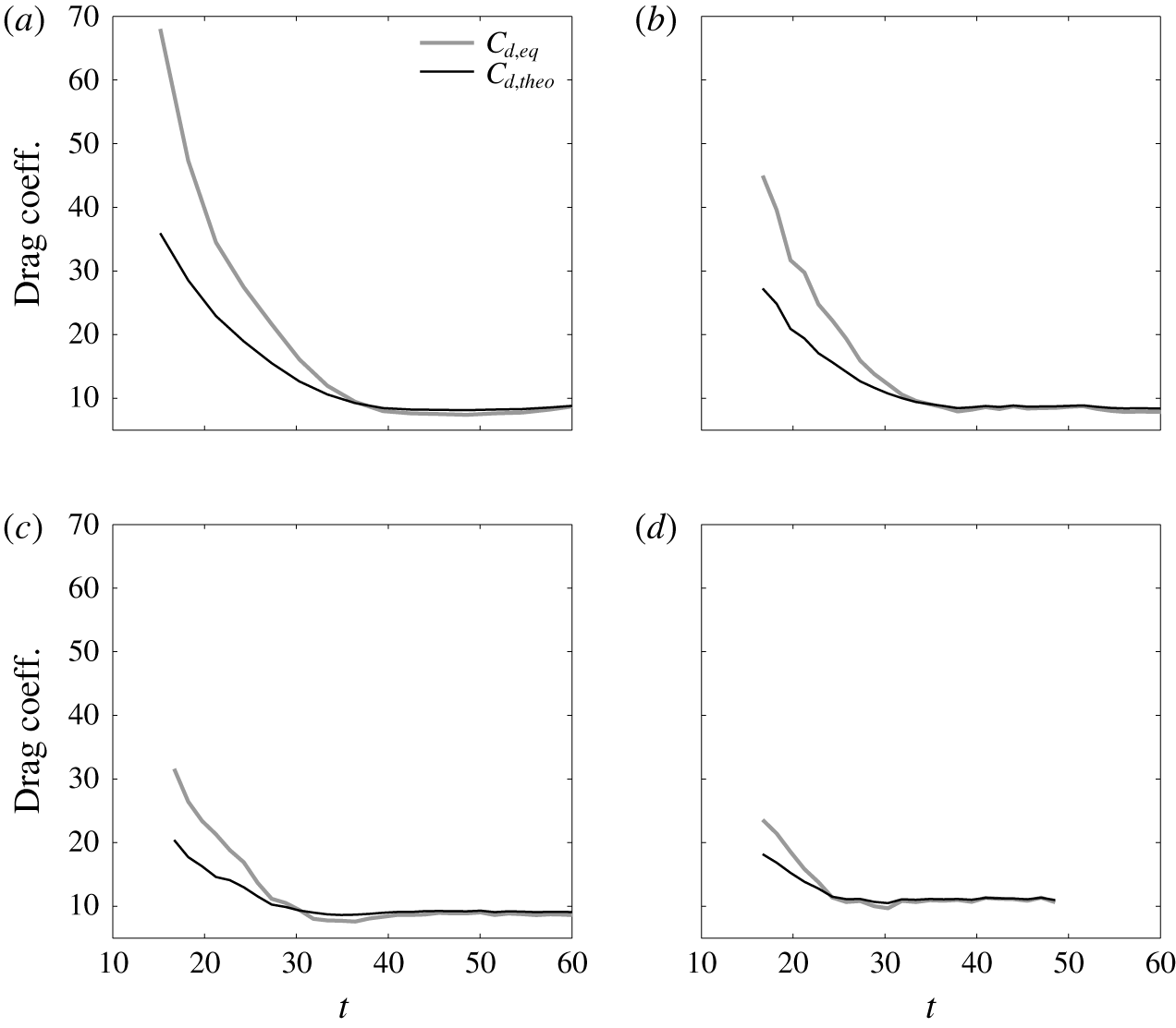
As shown in figure 13, the descending speed decreases over time at similar rates in all three cases after the terminal speed is attained, which indicates that the effect of particle size is negligible during this final stage. However, one may anticipate that the effect of particle size can become significant at a much later stage when the falling speed of the ring continues to drop to a value similar to the magnitude of  $w_{s}$. For example, in addition to the ring, swarms formed by falling particles might be seen (Bush, Thurber & Blanchette Reference Bush, Thurber and Blanchette2003). The discussion thus far regarding the effects of the particle size indicates the final stage does not vary significantly among cases with different sizes, such that the drag model presented in § 4 for the base case should be applicable to cases with all particle sizes as long as
 $w_{s}<U$. This is demonstrated in figure 15, which presents time histories of various drag coefficients for cases d03C084, d07C084, d10C084 and d14C084. It can be seen that time histories of
 $C_{d,eq}$ in all cases follow the same trend as in the base case.
6 Prediction of drop’s descending speed
Assuming a spherical shape for the drop and a thermal equilibrium state (as demonstrated in figure 8) such that the buoyant effect is only due to the presence of suspended particles, substitution of (4.13) into (4.2) yields a formula to predict the speed of the descending drop, i.e.,
 $$\begin{eqnarray}V_{h,pred}={\displaystyle \frac{1}{24}}{\displaystyle \frac{1}{\unicode[STIX]{x1D708}}}\unicode[STIX]{x1D6FE}\unicode[STIX]{x1D719}gD^{2},\end{eqnarray}$$
or a dimensionless relationship
 $$\begin{eqnarray}{\displaystyle \frac{\unicode[STIX]{x1D708}V_{h,pred}}{a^{2}g}}={\displaystyle \frac{1}{6}}\unicode[STIX]{x1D6FE}\unicode[STIX]{x1D719}.\end{eqnarray}$$
To demonstrate the predictability of (6.2), additional cases with various initial concentrations  $\unicode[STIX]{x1D719}_{0}=2.1\times 10^{-4}$,
 $4.2\times 10^{-4}$ and
 $16.8\times 10^{-4}$ of suspended particles are simulated, which are named d05C021, d05C042 and d05C168, respectively, as shown in table 1. Moreover, to test a different thermal condition, two additional cases using
 $\unicode[STIX]{x1D719}_{0}=4.2\times 10^{-4}$ and
 $8.4\times 10^{-4}$ with
 $d_{0}=5~\unicode[STIX]{x03BC}\text{m}$ and a half initial temperature difference between the lower and upper layers, i.e.,
 $T_{r,up}=28^{\circ }$ and
 $T_{r,low}=16$, are tested, which are named d05C042T2 and d05C084T2, respectively. To obtain a proper wavelength
 $\unicode[STIX]{x1D706}$ for single-mode perturbation, we run an additional multi-mode simulation to examine the most unstable mode. As presented in appendix B, a scaling
 $\unicode[STIX]{x1D706}\sim 12$ consistent to the base case can still be found, which is then used as the length of the initial perturbation in these two cases of the different initial temperature difference. Because
 $L\propto \left(\unicode[STIX]{x2202}T/\unicode[STIX]{x2202}z\right)^{-1/4}$, the consistent scaling rule in the present cases of two different initial temperature differences also indicates that the wavelength becomes larger as the temperature gradient decreases, which leads to a greater drop size and, according to (6.1), may increase the descending speed of the drop. It should be noted that due to the highly diffusive nature of the temperature, the interfacial thickness of the background temperature evolves with time and may vary among numerical and laboratory experiments. Different values of thickness result in different temperature gradients in the interfacial region, which alter the drop’s size, as previously mentioned. However, because here we include the comparison of the different temperature gradient, and the velocity for comparison is normalized with the drop’s size (i.e., equation (6.2)), the effect of the interfacial thickness (i.e., changing the temperature gradient and the drop’s size) can be implied from the current discussion.
Time histories of various drag coefficients in cases d03C084 (a), d07C084 (b), d10C084 (c) and d14C084 (d).

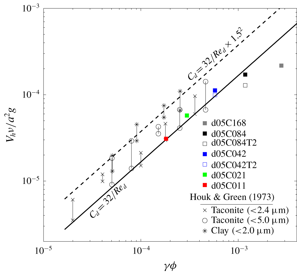
Normalized descending speed of drops from Houk & Green (Reference Houk and Green1973) and present simulation cases against  $\unicode[STIX]{x1D6FE}\unicode[STIX]{x1D719}$ along with the theoretical prediction by our drag model, equation (6.2) (black solid line), and its modification (black dashed line) considering the possible underestimation of the drop size in the laboratory experiments by Houk & Green (Reference Houk and Green1973). The vertical bars in the laboratory data points indicate the range of data variations in the measurement.

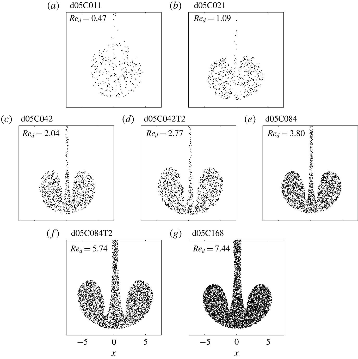
Snapshots of particles in the descending drop at the central slice in the $y$-direction at the time point when the drop reaches its maximum descending speed in all of the simulation cases presented in figure 16. Point markers are used to represent particles located at in
 $L_{y}/2-\unicode[STIX]{x1D6FF}y\leqslant y\leqslant L_{y}/2$, in which
 $L_{y}$ is the domain size in the
 $y$-direction and
 $\unicode[STIX]{x1D6FF}y$ is the grid size in the
 $y$-direction.

Figure 16 compares data from the present numerical cases with the prediction by (6.2). Because (6.2) assumes a buoyant force totally exerted by the suspended particles, for the present numerical results, data points presented in figure 16 are obtained when drops attain their maximum speeds, which are the time points at which the temperature exchange between the drop and ambient flows almost ceases (see § 3.2). As shown in figure 16, except at the larger values of  $\unicode[STIX]{x1D6FE}\unicode[STIX]{x1D719}$ (i.e.,
 ${>}2\times 10^{-3}$), the prediction of (6.2) is fairly close to the data points from present simulation results. The slight discrepancies between the numerical results and (6.2) are due to the fact that drops can deviate from a spherical shape during descent, which is discussed in detail in § 3. The deviation depends on the drop Reynolds number
 $Re_{d}$. To see this, figure 17 shows snapshots of particles at the central slice in the
 $y$-direction at time points when drops in all simulation cases presented in figure 16 reach their maximum
 $V_{h}$, along with the instantaneous
 $Re_{d}$. It shows that in small
 $Re_{d}$, drops retain a more spherical shape, whereas in large
 $Re_{d}$, drops (or heads of plumes) tend to be more oblate or hemispherical. In cases of large
 $Re_{d}$, the significant deviation from the spherical shape leads to the discrepancy between the actual
 $V_{h}$ and prediction by (6.2).
In addition to the present numerical cases, experimental data from Houk & Green (Reference Houk and Green1973) are also included for comparison. Although other data sets on double-diffusive sedimentation are also available, such as Green (Reference Green1987) and Parsons & Garcia (Reference Parsons and Garcia2000), Houk & Green (Reference Houk and Green1973) is found to be the only one that considers the size of the drops. The experimental set-up of Houk & Green (Reference Houk and Green1973) is very similar to the present cases except that the temperature difference between the upper and lower layers in each experimental case ranges from  $4.7\,^{\circ }\text{C}$ to
 $15.0\,^{\circ }\text{C}$. Three different sediment properties were tested: clay with
 $d_{0}<2~\unicode[STIX]{x03BC}\text{m}$, sorted taconite with
 $d_{0}<2.4~\unicode[STIX]{x03BC}\text{m}$ and taconite with
 $d_{0}<5.0~\unicode[STIX]{x03BC}\text{m}$. Houk & Green (Reference Houk and Green1973) found that the descending speed of the double-diffusive sedimentation drop is not a function of the thermal condition. Based on force balance, they suggest a relationship similar to (6.2) with an undetermined leading coefficient in the right-hand side rather than one sixth. Figure 16 also compares data points from Houk & Green (Reference Houk and Green1973) with the prediction by (6.2), which indicates a fair prediction by (6.2) because it covers the lower bound of the data set. The slight underestimation by (6.2) relative to the experimental data may be attributed to the fact that in Houk & Green (Reference Houk and Green1973), a universal value
 $a=1~\text{mm}$ was used in all data points because it is the measured finger radius. It is not certain how Houk & Green (Reference Houk and Green1973) exactly define their finger radius. However,
 $a$ increases during the development of the drop, and according to the present simulation results, the drop size during the detachment can be 1.2–1.5 times greater than the original finger size. Therefore, for comparisons with the experimental data, it may be fair to add a correction by multiplying by
 $1.5^{2}$ to compensate for the underestimation of the drop’s size in the laboratory experiments. As shown in figure 16, equation (6.2) and its corrected version (by multiplying
 $1.5^{2}$ to the right-hand side) are able to cover nearly the entire range of the data and show a good prediction for the experimental results.
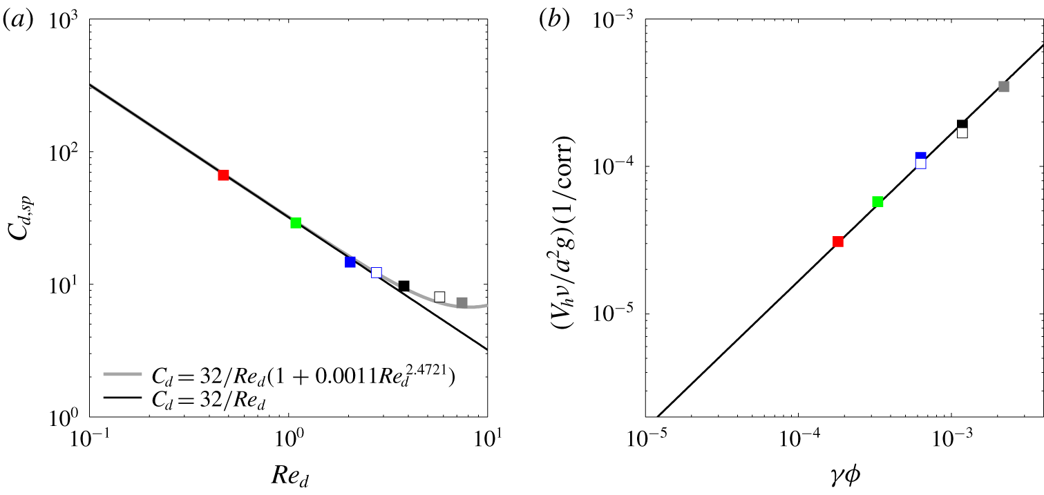
To this end, it might be worthwhile to add a correction, as a function of  $Re_{d}$, to our drag model when predicting for the case of larger
 $Re_{d}$. This can be simply done by plotting the drag coefficient estimated using (4.14) (i.e., assuming a spherical shape) against
 $Re_{d}$ to obtain a regression relation. This is shown in figure 18(a), in which we can obtain a corrected drag model for cases of larger
 $Re_{d}$ in the present numerical cases by regression, which reads
 $$\begin{eqnarray}C_{d,corr}={\displaystyle \frac{32}{Re_{d}}}(1+0.0011Re_{d}^{2.4721}).\end{eqnarray}$$
When comparing (6.3) with our results for the velocity prediction (i.e., equation (6.2)), it is equivalent to add the correction in (6.3) to the denominator of the left-hand side of (6.2). This is shown in figure 18(b), from which we obtain a significantly improved prediction for larger  $\unicode[STIX]{x1D6FE}\unicode[STIX]{x1D719}$. However, it should be noted that while we use very few data points for regression and apply for the current range of
 $Re_{d}$ (
 $O(1){-}O(10)$), for a more universal prediction for the case of large
 $Re_{d}$, many more data points at large
 $Re_{d}$ are needed. Here, we demonstrate the good predictability of our drag model for the drop’s speed in the case of small
 $Re_{d}$. The practical issue while applying our drag model is its dependency of the drop’s size, which typically requires small-scale measurement. In fact, the drop’s size arises from the initial perturbation, the size of which, as shown in appendix B, scales with the double-diffusion length scale
 $L$. That is, without measurement of the micro structures of the sediment-laden interface to obtain the size of drops or fingers, their size may be estimated by the external stratified condition (i.e., the temperature gradient). With the estimated length scales given by thermal conditions, predictions of the drop’s descending speed can be achieved with our drag model.
(a) Drag coefficients as a function of the drop Reynolds number  $Re_{d}$ in the present cases at the time point when the drop reaches its maximum descending speed along with the theoretical predictions by the original (black solid line) and the modified drag models (grey solid line). (b) Corrected non-dimensional maximum
 $V_{h}$ as a function of
 $\unicode[STIX]{x1D6FE}\unicode[STIX]{x1D719}$ in cases of various
 $Re_{d}$, in which ‘
 $\text{corr}=1+0.0011Re_{d}^{2.4721}$’ in the label of the
 $y$-axis and the black solid line represents
 $1/6(\unicode[STIX]{x1D6FE}\unicode[STIX]{x1D719})$, as in figure 16.

Schematic showing the polar coordinate in the spherical drop and the plume during the later stage of evolution, which is divided into regions of the body, stem and drop.

7 Difference between particle-laden and salt fingers: the effect of diffusivity
The formation and pinch-off of drops and rings presented here is most likely to occur in natural environments with suspended particles, but it may not be likely for dissolved concentrations, such as salt, because the greater diffusivity can prevent the occurrence of pinch-off, and because the stem connecting the bulbous head and the parent finger can be more persistent. To show this, we give a simple theoretical argument on the mass balance between the stem and the bulbous head. As shown in figure 19, we divide the finger in the later stage into the body, the stem, and the drop. For a stem with length  $l$ and cross-sectional area
 $A(z)$, neglecting the diffusive flux on the lateral side of the plume for the sake of simplicity, it is straightforward to write the equation of mass balance for a concentration field
 $C$ as
 $$\begin{eqnarray}{\displaystyle \frac{\text{d}}{\text{d}t}}\int _{l}\iint _{A}C(x,y,z)\,\text{d}x\,\text{d}y\,\text{d}z=-\boldsymbol{F}_{top}+\boldsymbol{F}_{btm},\end{eqnarray}$$
where
 $$\begin{eqnarray}\boldsymbol{F}=\iint _{A}\boldsymbol{u}_{rel}(x,y,z)C(x,y,z)\,\text{d}x\,\text{d}y\end{eqnarray}$$
is the mass flow rate, the subscripts  $top$ and
 $btm$ represent the top and bottom boundaries of the control volume (see figure 19), respectively, and
 $\boldsymbol{u}_{rel}$ in (7.2) is the velocity relative to the boundaries of the stem, which deforms and translates. During the late stage of finger development, the falling speed of the drop exceeds the transport velocity at the junction between the stem and the parent finger (
 $top$ in (7.1)). Hence, the mass transport within the stem is dominated by the movement of the connected drop, and the first term on the right-hand side of (7.1) can be neglected. Now, if one sets the top boundary to be fixed and the bottom boundary, located at the junction between the stem and the drop, to follow the descending head (i.e.,
 $\text{d}l/\text{d}t=V_{h}$), neglecting
 $\boldsymbol{F}_{top}$, equation (7.1) can be simplified to
 $$\begin{eqnarray}{\displaystyle \frac{\text{d}}{\text{d}t}}(\widetilde{\overline{C}A})={\displaystyle \frac{1}{l}}(-V_{h}\overline{C}A|_{btm}+\boldsymbol{F}_{btm}),\end{eqnarray}$$
where the tilde represents the averaged quantity over the vertical  $l$, and the overbar is the cross-sectional average. Within the control volume, retaining
 $\text{d}(\widetilde{\overline{C}A})/\text{d}t<0$ means that pinch-off of the drop will occur. For the drop with a volume
 $\unicode[STIX]{x1D6FA}$, again, neglecting the mass loss due to lateral diffusion, one can write a mass-balance equation as
 $$\begin{eqnarray}{\displaystyle \frac{\text{d}}{\text{d}t}}(\unicode[STIX]{x1D6FA}{\hat{C}})=-\boldsymbol{F}_{btm},\end{eqnarray}$$
where the overhat indicates the volumetric average. Equation (7.3) shows that movement of the head (i.e.,  $V_{h}$) and the relative mass flux are the two factors that lead to pinch-off. Moreover, equations (7.3) and (7.4) demonstrate the critical role of the relative mass flux (
 $\boldsymbol{F}_{btm}$) at the bottom end of the stem in dominating the late stage of plume dynamics. For example, an upward relative mass flow (i.e.,
 $\boldsymbol{F}_{btm}>0$) decelerates the pinch-off. In this case, equation (7.4) shows that the bulk mass in the head decreases with time, which further reduces the descending speed
 $V_{h}$ and also decelerates the pinch-off. As a result, it is possible that the head vanishes before the pinch-off can occur, particularly when
 $C$ is dilute.
Relative mass flow rates,  $\boldsymbol{F}$, of the drop in (a) the particle-laden finger and (c) the salt finger and the corresponding streamlines superimposed over (b) particles and (d) the normalized concentration field at the central slice in the
 $y$-direction at
 $t=33.37$. The crosses correspond to the point at which the velocity in the stem is equal to
 $V_{h}$, which are taken as positions of the conjunction between the stem and the drop. The figure shows the difference in the drop geometry between the particle-laden and salt fingers, and the latter case corresponds to an inflow mass flux to the stem, which delays the pinch-off of drops. The triangles in panels (b,d) indicate a wake region near the bottom of the stem. The point markers in panel (b) are used to represent the relative size difference between the cases and positions of the particles located in
 $L_{y}/2-\unicode[STIX]{x1D6FF}y\leqslant y\leqslant L_{y}/2$, in which
 $L_{y}$ is the domain size in the
 $y$-direction and
 $\unicode[STIX]{x1D6FF}y$ is the grid size in the
 $y$-direction.

Time histories of the descending speed  $V_{h}$ in a salt finger (grey solid line), the single-phase simulations for
 $w_{s}=3.33\times 10^{-2}$ with
 $Sc_{\unicode[STIX]{x1D719}}=6.67\times 10^{2}$ (dashed line) and
 $Sc_{\unicode[STIX]{x1D719}}=6.67\times 10^{3}$ (dash-dotted line), and the base case (solid line with circular markers).

To compare with salt fingers, we also run the salinity case with an initial concentration of  $s_{0}=1.848$ psu, which results in the same bulk density as the present particle-laden case. The salinity field
 $s$ is simulated by solving the governing equation
 $$\begin{eqnarray}\frac{\unicode[STIX]{x2202}s}{\unicode[STIX]{x2202}t}+\boldsymbol{u}_{c}\boldsymbol{\cdot }\unicode[STIX]{x1D735}s=\unicode[STIX]{x1D705}_{s}\unicode[STIX]{x1D6FB}^{2}s,\end{eqnarray}$$
with the diffusivity  $\unicode[STIX]{x1D705}_{s}=1.5\times 10^{-9}~\text{m}^{2}~\text{s}^{-1}$. Figure 20 shows representative snapshots of the plume in the later stage (
 $t=33.37$) superimposed with the instantaneous streamlines and the corresponding bulk mass fluxes relative to the descending drop in cases of particle-laden and salt fingers. One can define the point of zero velocity (i.e., the rear stagnation point relative to the motion) at the centre of the plume (see crosses in figure 20b,d) as the bottom boundary of the stem. As shown in figure 20(a), the profiles of the bulk mass flux show a relative mass flux of nearly zero at the bottom of the stem, which means that in (7.3),
 $\boldsymbol{F}_{btm}\approx 0$ and
 $\widetilde{\overline{C}A}$ continues to decrease over time. Nevertheless, for the salt-finger case, figure 20(c) shows a significant upward (positive) mass flux at the bottom (marked by green crosses). The strong upward flux in the latter case is induced by the diffusive nature of the salinity field. At the downwind side of the drop, the diffused mass is further transported upward relative to the descending drop due to the wake generated at the rear of the drop. The influence of the wake region in the two cases can be distinguished qualitatively from figure 20(b,d), in which the wake regions near the bottom of the stem are highlighted with triangles. The figures show that while very few particles are found in the highlighted wake region in the particle-laden case (see figure 20b), the wake region in the salt-finger case contains a certain portion of the concentration. This leads to continuous drainage of salinity from the drop into the stem, which in turns decelerates the pinch-off of the bulbous head.
The detrainment from the drop due to the wake can be demonstrated more specifically by performing simulations with the conventional scalar-limit approximation (e.g., Yu et al. Reference Yu, Hsu and Balachandar2014; Burns & Meiburg Reference Burns and Meiburg2015) with artificial diffusivity. The dimensional governing equation for the concentration  $\unicode[STIX]{x1D719}$ of the particles is written as
 $$\begin{eqnarray}\frac{\unicode[STIX]{x2202}\unicode[STIX]{x1D719}}{\unicode[STIX]{x2202}t}+\boldsymbol{u}_{c}\boldsymbol{\cdot }\unicode[STIX]{x1D735}\unicode[STIX]{x1D719}-W_{s}{\displaystyle \frac{\unicode[STIX]{x2202}\unicode[STIX]{x1D719}}{\unicode[STIX]{x2202}z}}=\unicode[STIX]{x1D705}_{\unicode[STIX]{x1D719}}\unicode[STIX]{x1D6FB}^{2}\unicode[STIX]{x1D719},\end{eqnarray}$$
where  $W_{s}$ is the dimensional Stokes’ settling velocity and
 $\unicode[STIX]{x1D705}_{\unicode[STIX]{x1D719}}$ is the diffusivity. Here, we run two cases of
 $\unicode[STIX]{x1D705}_{\unicode[STIX]{x1D719}}=1.5\times 10^{-9}$ and
 $1.5\times 10^{-10}~\text{m}^{2}~\text{s}^{-1}$ with
 $w_{s}$ the same as in the base case (see cases SP1 and SP2 in table 1, respectively). The simulation set-ups in these two cases are the same as that in the base case, except that the discrete particles in the base case are replaced with a continuum concentration
 $\unicode[STIX]{x1D719}$. We do not use an even lower
 $\unicode[STIX]{x1D705}_{\unicode[STIX]{x1D719}}$ value because
 $\unicode[STIX]{x1D705}_{\unicode[STIX]{x1D719}}=1.5\times 10^{-10}~\text{m}^{2}~\text{s}^{-1}$ nearly reaches the limit of the diffusivity due to the grid resolution (i.e., numerical diffusion
 ${\sim}O(10^{-11}~\text{m}^{2}~\text{s}^{-1})$). Figure 21 shows the time histories of the three single-phase cases and that of the base case for comparison. It can be seen that the effect of the aforementioned detrainment due to the wake becomes important as time increases. The resulting dilution in the drop results in an 8.9 % reduction of the terminal speed in case SP2 and a 16.3 % reduction in case SP1. According to (4.2), an estimation gives approximately 17.0 % and 30.0 % reduction in buoyancy before the terminal speed is reached in cases SP2 and SP1, respectively, because the size of the drop does not vary among these cases. In figure 21, the reduction in the terminal speed is more pronounced in the salt-finger case because, without
 $w_{s}$, the drop in the salt-finger case evolves at a slower rate (i.e., a lower
 $V_{h}$), as discussed in § 5.
To sum up at this point, while the gravitational settling of particles enhances the formation of the drop, the longer duration to reach a state of thermal equilibrium in the salt-finger case can lead to a significant loss of the salinity mass in the drop due to the combined effects of the diffusive nature and flow wake at the rear of the drop. This can make the present results of formation and evolution of the particle-laden drop less significant in the salt-finger case. This is consistent with the early experimental study by Green (Reference Green1987), who found significantly lower descending speeds of drops in salt fingers than in the particle-laden case under the same buoyant and thermal conditions in the bulk. As a whole, one may expect that the vertical mass flux that arises from double-diffusive sedimentation can be much stronger than its salt-finger counterpart. Moreover, strong vertical mass fluxes could lead to secondary instabilities and flow fluctuations that further mix both the particle concentration and background temperature, thus forming a layered structure along the vertical direction (Radko Reference Radko2013). While the layer formation in double-diffusive sedimentation was first discussed in Reali et al. (Reference Reali, Garaud, Alsinan and Meiburg2018) for the cases of the intermediate diffusivity ratio, the present cases in which the ratios are infinitesimally small deserve future study.
8 Concluding remarks
Numerical simulations are conducted for detailed investigation of the formation of drops and vortex rings of particle-laden fingers in double-diffusive convection in a stable background stratification induced by temperature. The initial perturbation at the particle-laden interface grows due to the rapid thermal exchange between the perturbation and the ambient fluid. In the lower region of the domain, this makes the perturbed particle-laden fluid parcel heavier than the surrounding fluid, a phenomenon known as double-diffusive sedimentation. After the head of the particle-laden fluid passes the region of the temperature gradient and reaches the layer of uniform temperature, the density anomaly gradually vanishes, and the head undergoes an acceleration phase, which transforms the bulbous head into a drop connected to its parent finger by a stem. During this acceleration stage, the sphere-like particle-laden drop is subject to an oblate perturbation, which leads to the disappearance of the stem (i.e., pinch-off of the drop) and entrainment in the top region of the drop. The drop reaches its terminal speed when the temperature perturbation completely vanishes, at which time the drop becomes a buoyant vortex ring associated with significant lateral expansion. The drop then enters a deceleration phase whose motion follows the similarity assumption.
A theoretical drag model is presented for prediction of the drop velocity. The model is obtained from the solution of creeping flow over a spherical drop by applying the boundary condition for the vorticity field, rather than the velocity in previous studies. The resulting formulation of the drag coefficient is a general form applicable to various cases of the boundary condition. In conjunction with the present simulation results, this theoretical drag model shows good agreement with the simulation results, especially when the drop becomes spherical and the later stage of a ring torus. Moreover, we investigate five particle sizes to examine the effects of the settling velocity and find that the rapid settling associated with larger particles enhances vertical transport, accelerating the formation of the drop and its detachment from the finger. The resulting greater descending speed of the drop enhances thermal exchange between the drop and the surrounding fluid, which causes the drop to reach its terminal speed earlier. However, due to the same bulk density anomaly of suspended particles in the drop, the terminal speed and the subsequent decrease in the descending speed do not differ significantly among the various particle sizes. We also found that the results of a drop’s descending speed with different particle sizes converge when the size decreases. The drag model is then applied to predict the drop’s speed. The comparison with the simulation results under different bulk conditions and the previous experimental results shows good model predictability for the descending speed of drops, particularly in the case of a small drop Reynolds number, for which the particle-laden drop takes more of a spherical shape. Finally, the differences between the salt finger and the present particle-laden cases are discussed. The diffusive nature of the dissolved scalar field, along with the wake effect, can result in an apparent loss of mass from the drop and a more permanent presence of the stem, which connects the drop with the parent finger. This makes the present results of the drop detachment much less likely to occur in the salt finger.
To our knowledge, this paper presents the first EL simulation of particle-laden fingers in double-diffusive sedimentation. Due to the very low diffusivity associated with suspended particles in nature, the present Lagrangian particles can be a more relevant representation than the conventional scalar approach, in which an overly diffusive nature cannot be avoided in the numerical simulation. Our detailed investigation and analysis of the simulation results help obtain a better understanding of the sedimentation process of suspended materials near the surface of natural water bodies (e.g., oceans and lakes), which are usually stratified water columns due to temperature or salinity. The finding that the drop finally undergoes its deceleration (or dissipation) phase may imply the lack of importance of double-diffusive convection in enhancing sedimentation to form underwater turbidity currents (Hizzett et al. Reference Hizzett, Hughes Clarke, Sumner, Cartigny, Talling and Clare2018). However, our results can have critical implications for hydrodynamic influences on particle–particle interactions, such as collision and aggregation. The interaction of hydrodynamics with the flocculation process, leading to an enhancement of particle settling, is certainly deserving of future exploration.
Acknowledgements
The authors gratefully acknowledge the support of the Taiwan Ministry of Science and Technology (MOST) Civil and Hydraulic Engineering Program under grant no. 106-2628-E-002-016-MY4, the Ministry of Education (MOE) Higher Education Sprout Project in Taiwan (NTU Core Consortium: 108L880206), and National Taiwan University career development project (NTU-CDP-108L7720). The computation was performed on the Dell PowerEdge M620 supercomputer cluster located at Taida Institute of Mathematical Science at National Taiwan University, which is gratefully acknowledged.
Declaration of interests
The authors report no conflict of interest.
Appendix A
To examine the importance of particle collision, we run an additional case in which the collision model is turned on. In the present numerical model, a standard soft-sphere collision model by Cundall & Strack (Reference Cundall and Strack1979) is used to model particle–particle collisions, the details of which can be found in Chou et al. (Reference Chou, Gu and Shao2015) and Chang et al. (Reference Chang, Chiu, Hung and Chou2019). Here, we assume a small value for the coefficient of restitution  $e=0.01$, which represents a nearly inelastic collision between particles. Because particles almost stick to each other while colliding, this set-up can be seen as a very simplified flocculation model. Except for the consideration of the particle collision and the difference in the initial positions of particles assigned randomly, all other parameters and the numerical set-up are the same as those in the base case d05C084. This case is named d05C084col. Comparison of the descending speed
 $V_{h}$ of the drop from cases d05C084 and d05C084col in figure 22 shows no significant difference in bulk behaviour between these two cases. Moreover, figure 23 presents the statistical results of numbers of grid cells versus numbers of particles contained in the grid cell at the time instant
 $t=40.96$ when the drops reach their maximum speed. In this figure, if the inelastic collision is important, we anticipate that the histogram of case d05C084col would shift to the right relative to case d05C084. However, this is not seen in figure 23, and very little difference between the two cases can be found. The insignificant effect of collision in the present range of concentration (i.e., most cases
 ${<}10^{-3}$ in volume fraction) was suggested in previous studies (Elghobashi & Truesdell Reference Elghobashi and Truesdell1993; Balachandar & Eaton Reference Balachandar and Eaton2010) in the context of dispersive turbulent two-phase flows. Also, in the same concentration range, Green (Reference Green1987) suggested an insignificant effect of particle–particle interaction (i.e., coagulation). Therefore, we disregard particle–particle interactions in this study.
Time histories of the descending speed  $V_{h}$ of the plume head in cases d05C084 (base) and d05C084col.

Histograms of numbers of grid cells versus numbers of particles contained in the grid cell at the time instant  $t=40.96$ in cases d05C084 and d05C084col when drops reach the maximum speed (see figure 22).

Representative snapshots of the particle-laden fingers at the central slice in the  $y$-direction in the multi-mode cases with the same physical set-up as in cases d05C084 (a) and d05C084T2 (b) and the corresponding spectrum of the volume concentration
 $\unicode[STIX]{x1D719}$ sampled at central slice in the vertical direction (
 $z=0$) at three representative time instants (c,d) to obtain the most energetic modes. The dotted lines in (c) (
 $k=0.22$) and (d) (
 $k=0.26$) represent the theoretical values of the dominant modes for the RTI case, in which the background temperature gradient vanishes.

Appendix B
To obtain a relevant wavelength ( $\unicode[STIX]{x1D706}$) for the present single-mode perturbation (2.16), we run a case in a domain with the horizontal size larger and the vertical size shorter than the present single-mode case. The domain size is given by
 $L_{x}\times L_{y}\times L_{z}=270\times 270\times 90$. The domain’s shorter vertical size is chosen because we only aim to obtain the most energetic unstable mode of the early development of the double-diffusive fingers. The grid resolution is
 $384\times 384\times 128$. The particle size of the base case
 $d_{0}=5~\unicode[STIX]{x03BC}\text{m}$ is used. Initially, the particles are randomly assigned in the upper half-region of the domain such that the bulk volumetric concentration is
 $\unicode[STIX]{x1D719}_{0}=8.4\times 10^{-4}$, following Green & Schettle (Reference Green and Schettle1986). We run two cases with the same physical set-up as in cases d05C084 and d05C084T2 except for the initial perturbation. Here, without imposing additional perturbations to the bulk flow, the infinitesimal perturbations due to the randomness and discreteness of the particle distribution can lead to multi-mode double-diffusive fingers, as shown in figure 24(a,b), in which we show instantaneous snapshots of the particles at the central slice in the
 $y$-direction. Figure 24 shows the time evolution of the spectrum of
 $\unicode[STIX]{x1D719}$ at
 $z=0$, from which we can see the most energetic modes range roughly from the wavenumber
 $k=0.4$ to
 $0.6$ in both cases. Therefore, we use the perturbation wavelength
 $\unicode[STIX]{x1D706}=12$, corresponding to
 $k=0.52$, for the present single-mode perturbation. In addition, we plot values of the dominant modes for the RTI case, in which the background temperature gradient vanishes, as shown by the dotted lines in figure 24(c,d). These are obtained from the theoretical results in Chandrasekhar (Reference Chandrasekhar1961) and then rescaled with the double-diffusion length scale
 $L$. Figure 24(c,d) show that the dominant RTI modes are less than half of the present dominant modes in both cases, which indicates the dominance of the double-diffusive sedimentation in the present cases. A more detailed derivation for the transition between RTI and double-diffusive convection of the instability modes can be found in a recently submitted paper by Chou et al. (Reference Chou, Cheng, Chen and Hung2019).
Appendix C
To obtain the solution for the Oseen equations for the present case of the particle-laden drop, we solve
 $$\begin{eqnarray}\displaystyle & \displaystyle \boldsymbol{V}_{h}\boldsymbol{\cdot }\unicode[STIX]{x1D735}\boldsymbol{u}=-\unicode[STIX]{x1D735}p+\unicode[STIX]{x1D707}\unicode[STIX]{x1D6FB}^{2}\boldsymbol{u}, & \displaystyle\end{eqnarray}$$
 $$\begin{eqnarray}\displaystyle & \displaystyle \unicode[STIX]{x1D735}\boldsymbol{\cdot }\boldsymbol{u}=0 & \displaystyle\end{eqnarray}$$
with the same boundary conditions given by (4.5)–(4.7). Following Chester, Breach & Proudman (Reference Chester, Breach and Proudman1969), in terms of the stream function, the inner expansion is written as
 $$\begin{eqnarray}\unicode[STIX]{x1D6F9}=\unicode[STIX]{x1D6F9}_{0}+Re_{d}\unicode[STIX]{x1D6F9}_{1}+Re_{d}^{2}\log Re_{d}\unicode[STIX]{x1D6F9}_{2L}+Re_{d}^{2}\unicode[STIX]{x1D6F9}_{2}+\cdots \,,\end{eqnarray}$$
which gives the vorticity field
 $$\begin{eqnarray}\unicode[STIX]{x1D714}=\unicode[STIX]{x1D714}_{0}+Re_{d}\unicode[STIX]{x1D714}_{1}+Re_{d}^{2}\log Re_{d}\unicode[STIX]{x1D714}_{2L}+Re_{d}^{2}\unicode[STIX]{x1D714}_{2}+\cdots \,.\end{eqnarray}$$
In (C 3), the zero-order approximation can be written as
 $$\begin{eqnarray}\unicode[STIX]{x1D6F9}_{0}={\displaystyle \frac{1}{2}}\left[r^{2}-J_{0}r-\left(1-J_{0}\right){\displaystyle \frac{1}{r}}\right]\sin ^{2}\unicode[STIX]{x1D703},\end{eqnarray}$$
which is obtained from the Stokes solution with the boundary condition
 $$\begin{eqnarray}\unicode[STIX]{x1D714}_{0}=-E_{0}\sin \unicode[STIX]{x1D703}\quad \text{on }|\boldsymbol{r}|=a,\end{eqnarray}$$
in which  $E_{0}$ is a constant and
 $J_{0}=E_{0}a/V_{h}$ (see § 4). Moreover, the first-order term in (C 3) can be written as
 $$\begin{eqnarray}\unicode[STIX]{x1D6F9}_{1}=C_{1}\unicode[STIX]{x1D6F9}_{0}+\unicode[STIX]{x1D6F9}^{\ast },\end{eqnarray}$$
where  $C_{1}$ is a coefficient to be matched with the outer solution (Proudman & Pearson Reference Proudman and Pearson1957) and
 $$\begin{eqnarray}\unicode[STIX]{x1D6F9}^{\ast }=F(r)\sin ^{2}\unicode[STIX]{x1D703}\cos \unicode[STIX]{x1D703}.\end{eqnarray}$$
The vorticity field due to  $\unicode[STIX]{x1D6F9}_{1}$ can be thus written as
 $$\begin{eqnarray}\unicode[STIX]{x1D714}_{1}=C_{1}\unicode[STIX]{x1D714}_{0}+G(r)\sin \unicode[STIX]{x1D703}\cos \unicode[STIX]{x1D703}.\end{eqnarray}$$
Now, it can be seen that the boundary condition (4.7) based on the observation of the present vorticity field (see figure 10) does not allow for a full description of the boundary condition for the first-order solution  $\unicode[STIX]{x1D6F9}_{1}$ (i.e., the second term on the right-hand side of (C 9)), which also applies for all the higher-order terms of (C 3) (Chester et al. Reference Chester, Breach and Proudman1969). However, the odd feature of (C 8) implies that
 $\unicode[STIX]{x1D6F9}^{\ast }$ does not contribute to the drag on the sphere. As a result, without seeking the value of
 $C_{1}$ by matching the the outer solution, one can argue that the resulting drag to the first-order approximation due to a combination of
 $\unicode[STIX]{x1D6F9}_{0}$ and
 $\unicode[STIX]{x1D6F9}_{1}$ becomes
 $$\begin{eqnarray}C_{d,Oseen}={\displaystyle \frac{16J_{0}(1+C_{1}Re_{d})}{Re_{d}}}.\end{eqnarray}$$
Because the boundary condition  $\unicode[STIX]{x1D714}=-E\sin \unicode[STIX]{x1D703}$ (equations (4.7) and (4.10)) are formulated for the total flow field, and given by (C 6) and (C 7), one can obtain
 $E=E_{0}(1+C_{1}Re_{d})$. Thus, equation (C 10) can be rewritten as
 $$\begin{eqnarray}C_{d,Oseen}={\displaystyle \frac{16J}{Re_{d}}},\end{eqnarray}$$
which is the same as the one obtained from the Stokes solution in the present study.