1 Introduction
Turbulent density currents are ubiquitous in geophysical, industrial, and environmental settings. Mixing, often driven and dominated by turbulence, plays a crucial role in the dynamics of these currents. Much effort has gone into the study of various examples of these flows. Clarke (Reference Clarke1972), along with Garvine & Monk (Reference Garvine and Monk1974), have studied naturally occurring sea-breeze fronts and saline estuary intrusions, analysing the density and velocity structure of such flows. Fay (Reference Fay, Carstens and McClimans1980) quantified the dilution of dense gas leaks released in accidents. Ivey, Winters & Koseff (Reference Ivey, Winters and Koseff2008) reviews measurements of vertical mixing in geophysical environments, and there is a growing literature on mixing in gravity currents (Hallworth et al. Reference Hallworth, Phillips, Huppert and Sparks1993; Liapidevskii Reference Liapidevskii1994; Johnson & Hogg Reference Johnson and Hogg2013; Samasiri & Woods Reference Samasiri and Woods2015; Sher & Woods Reference Sher and Woods2015; Kneller et al. Reference Kneller, Nasr-Azadani, Radhakrishnan and Meiburg2016; Sher & Woods Reference Sher and Woods2017).
The classic work of Ellison & Turner (Reference Ellison and Turner1959) measured mixing in gravity-driven flows experimentally. Their data was combined with a depth-averaged model to explore the effect of entrainment of ambient fluid into the flow as it migrated downstream. Ellison & Turner (Reference Ellison and Turner1959) recognised that the flow is in fact stratified with a vertical distribution of horizontal velocity and density as ambient fluid is mixed into the current. In their modelling they assumed that the structure of the stratification, as quantified by shape factors in the depth-averaged equations, is fixed.
Many works subsequent to Ellison & Turner (Reference Ellison and Turner1959) have explored and refined the parametrisation of the mixing (Strang & Fernando Reference Strang and Fernando2001; Cenedese & Adduce Reference Cenedese and Adduce2010) and have used the parametrisation to model mixing in environmental and geophysical flows (Bursik & Woods Reference Bursik and Woods1996; Xu et al.
Reference Xu, Chang, Peters, Özgökmen and Chassignet2006; Johnson & Hogg Reference Johnson and Hogg2013). For horizontal currents, the depth-averaged model parametrises the mixing in terms of a bulk Richardson number, based on the buoyancy
 $g^{\prime }$
, the depth
 $h$
and the velocity
 $u$
,
 $Ri_{b}=\unicode[STIX]{x0394}g^{\prime }h/u^{2}$
. For a horizontal current models typically assume the mixing reduces to very small values as the bulk Richardson number
 $Ri_{b}$
approaches or increases beyond 1/4.
Depth-averaged models are very useful, but most analytical modelling has been developed using the assumption that the shape factors are constant. In this work we take a different approach and examine some global constraints on the evolution of an initially uniform current of one density supplied to the base of a deep well-mixed layer of fluid of lower density. We assume that the flow migrates along a horizontal boundary and we allow for gradual mixing across the interface between the two fluids, which produces an upper interfacial mixing layer, which is stratified in velocity and density. Throughout this paper we refer to this stratified upper layer as the interfacial mixing layer. Eventually, if the interfacial mixing layer is able to grow sufficiently, it will spread through the whole depth of the lower layer. We assume that the mixing layer deepens until the gradient Richardson number is larger than 1/4 and calculate the associated entrainment and dilution of the flow as a function of the source Froude number. Motivated by experimental observations (Cenedese, Nokes & Hyatt Reference Cenedese, Nokes and Hyatt2016; Sher & Woods Reference Sher and Woods2017) and numerical simulations (Hogg et al. Reference Hogg, Nasr-Azadani, Ungarish and Meiburg2016; Kneller et al. Reference Kneller, Nasr-Azadani, Radhakrishnan and Meiburg2016), as a simplification we assume that the vertical profiles of horizontal velocity and buoyancy in the downstream flow involve a linearly stratified region overlying a uniform layer below. Later in this paper, figure 8 presents density and velocity data taken from a numerical simulation of a gravity current by Kneller et al. (Reference Kneller, Nasr-Azadani, Radhakrishnan and Meiburg2016). The profiles presented are consistent with our ansatz of a linearly stratified interfacial mixing layer overlying a uniform lower layer. We explore how the volume flux of the flow changes as a function of the gradient Richardson number of the stratified zone. Our results provide insight into the magnitude of dilution of dense horizontal currents, through mixing with ambient fluid, and provide a framework to help interpret predictions of mixing as derived from local models of entrainment.
We first present a general model of the mixing, and then in § 3 present results for the reference case in which we assume the downstream flow is well mixed and has uniform velocity and buoyancy (Johnson & Hogg Reference Johnson and Hogg2013). This reference case enables comparison of the mixing with that predicted by the new family of flows in which we include a linearly stratified region at the interface between the two fluids (§ 4). Furthermore, in § 5 we consider the case of more energetic flows in which all the injected fluid becomes modified through mixing and the whole current becomes linearly stratified in buoyancy and velocity. We refer to the layer as being fully modified in this case. We conclude by discussing the implications of these models for gravity currents and other density-stratified flows.
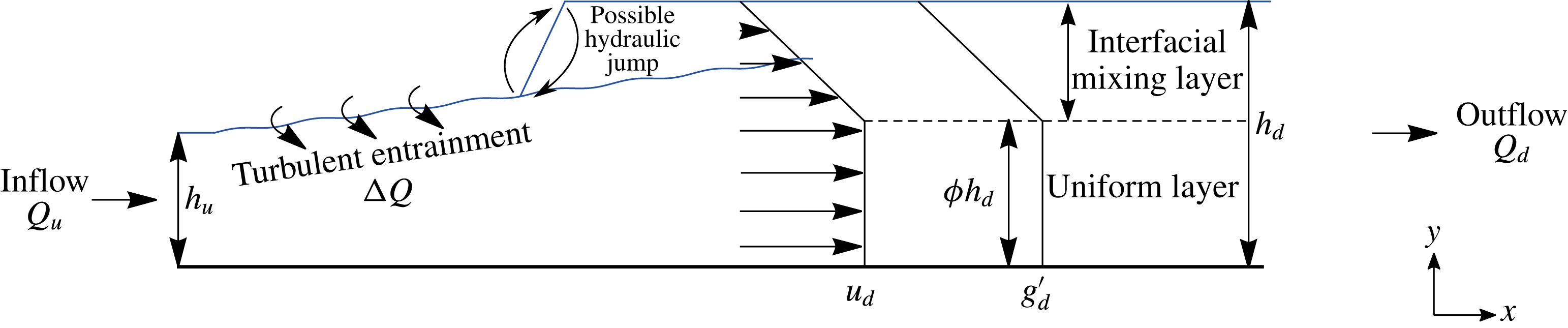
A schematic of the system under consideration. A uniform upstream profile at
 $x=0$
evolves to a hybrid uniform-linear downstream profile via turbulent entrainment through the interface and/or possibly through a hydraulic jump. The uniform flow fraction of the velocity and density profiles is given by
 $\unicode[STIX]{x1D719}\in [0,1]$
. The upstream volume flux is denoted
 $Q_{u}$
and the downstream volume flux is denoted
 $Q_{d}$
. In § 3 we have set
 $\unicode[STIX]{x1D719}=1$
such that only a uniform downstream profile is considered.

2 Model
Consider a steady two-dimensional, inviscid, layer of fluid of depth
 $h(x)$
, velocity
 $u(x,y)$
and buoyancy profile
 $g^{\prime }(x,y)$
. In this case
 $x$
is the along-stream direction and
 $y$
the vertical cross-stream direction. By considering a control volume and proceeding under the assumption that the pressure in the flow is hydrostatic and constant at some height
 $H>h$
, in the upper static layer, the conservation of vertical mass, momentum, and buoyancy requires that
 $$\begin{eqnarray}\displaystyle \left.\begin{array}{@{}c@{}}\displaystyle \frac{\unicode[STIX]{x2202}}{\unicode[STIX]{x2202}x}\left(\int _{0}^{h}u\,\text{d}y\right)=\unicode[STIX]{x1D700}u(x,h),\quad \frac{\unicode[STIX]{x2202}}{\unicode[STIX]{x2202}x}\left(\int _{0}^{h}u^{2}+\left(\int _{y}^{h}g^{\prime }\,\text{d}y^{\ast }\right)\,\text{d}y\right)=0,\\[10.0pt] \displaystyle \frac{\unicode[STIX]{x2202}}{\unicode[STIX]{x2202}x}\left(\int _{0}^{h}ug^{\prime }\,\text{d}y\right)=0,\end{array}\right\} & & \displaystyle\end{eqnarray}$$
where
 $\unicode[STIX]{x1D700}$
is an entrainment parameter. A generalised schematic of the system under consideration can be seen in figure 1. Throughout this paper we assume the upstream flow profile is uniform in velocity and buoyancy. Although we could generalise this initial condition, it corresponds to the mixing produced in the initial phases of a flow from a uniform source and represents a simple illustration of the approach. Downstream we allow the flow to become stratified and we assume that the buoyancy and momentum mix at the same rate, such that the depth of the velocity- and buoyancy-stratified zones are the same. We assume that the fluid transitions between the upstream and downstream state via turbulent entrainment and mixing through the interface, or possibly through a hydraulic jump from a supercritical to subcritical flow, or a combination of both. We define the averaged quantities
 $$\begin{eqnarray}\displaystyle S_{1}\bar{u}h=\int _{0}^{h}u\,\text{d}y,\quad S_{2}\bar{u}^{2}h+S_{3}\bar{g}^{\prime }h^{2}=\int _{0}^{h}u^{2}+\left(\int _{y}^{h}g^{\prime }\,\text{d}y^{\ast }\right)\,\text{d}y,\quad S_{4}\bar{u}\bar{g}^{\prime }h=\int _{0}^{h}ug^{\prime }\,\text{d}y, & & \displaystyle \nonumber\\ \displaystyle & & \displaystyle\end{eqnarray}$$
where
 $\bar{u}(x)$
and
 $\bar{g}^{\prime }(x)$
are the depth-averaged velocity and buoyancy profiles and
 $h(x)$
is the depth of the current. The shape factors
 $S_{1},S_{2},S_{3},S_{4}$
are defined in terms of the particular structure of the velocity and buoyancy profiles
 $u(x,y),g^{\prime }(x,y)$
. From these depth-averaged quantities and the conservation laws (2.1) we find that the transition from a uniform source at
 $x=0$
to the flow at a downstream location
 $x=x_{d}$
can be written in terms of the shape factors at
 $x=x_{d}$
in the form
 $$\begin{eqnarray}\displaystyle \left.\begin{array}{@{}c@{}}\displaystyle S_{1}u_{d}h_{d}-u_{u}h_{u}=\int _{0}^{x_{d}}\unicode[STIX]{x1D700}u(x,h)\,\text{d}x,\quad u_{u}^{2}h_{u}+\frac{g_{u}^{\prime }h_{u}^{2}}{2}=S_{2}u_{d}^{2}h_{d}+S_{3}g_{d}^{\prime }h_{d}^{2},\\[5.0pt] u_{u}g_{u}^{\prime }h_{u}=S_{4}u_{d}g_{d}^{\prime }h_{d},\end{array}\right\} & & \displaystyle\end{eqnarray}$$
where
 $u_{u}=\bar{u}(0),u_{d}=\bar{u}(x_{d}),g_{u}^{\prime }=\bar{g}^{\prime }(0),g_{d}^{\prime }=\bar{g}^{\prime }(x_{d}),h_{u}=h(0),h_{d}=h(x_{d})$
denote the upstream and downstream velocities, buoyancies, and heights of the flow, respectively.
We now investigate the possible flow solutions given a series of simplified vertical velocity and density profiles in the downstream flow. We start with a reference model in which we assume the downstream flow is well-mixed and vertically uniform, although noting that this flow structure is unstable. Then we consider the case in which the mixing leads to a linearly stratified interfacial mixing layer above a well-mixed uniform region at the base of the flow in which buoyancy is assumed to be equal to that of the upstream flow, as shown in figure 1.
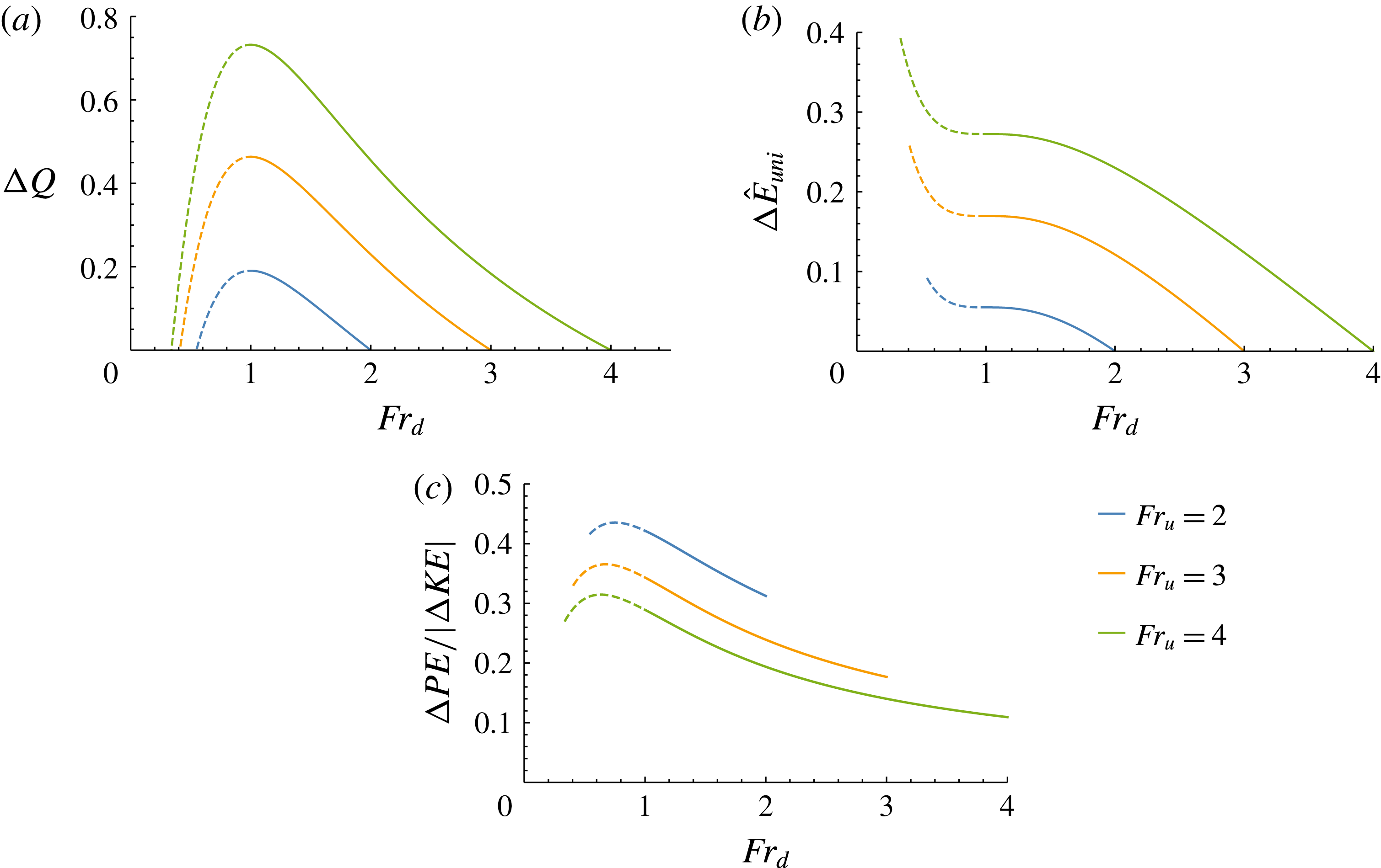
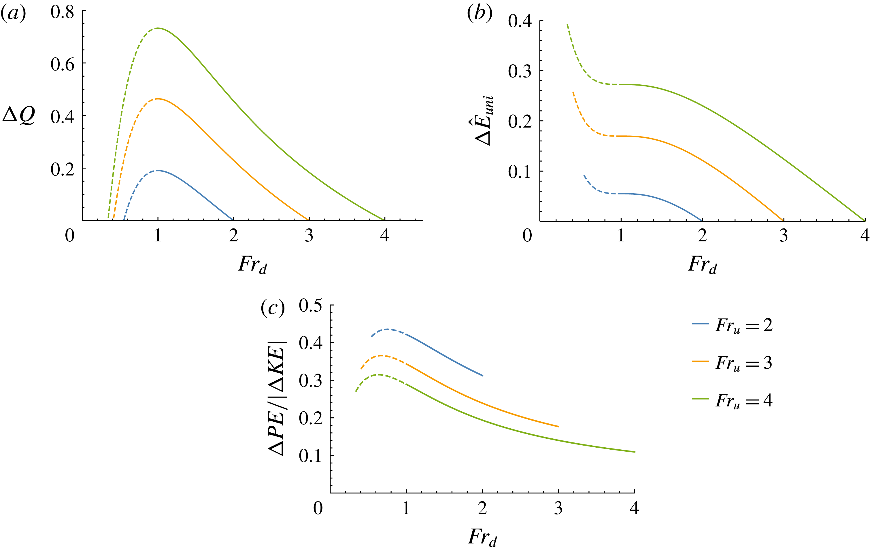
These figures refer to the case of vertically uniform buoyancy and horizontal velocity. (a) Mixing as a function of the downstream Froude number attained by the flow. The two roots occur at
 $Fr_{u}=Fr_{d}$
where no transition has occurred, and
 $Fr_{u}=Fr_{d}^{\ast }$
the conjugate hydraulic jump solution with no entrainment. Maximal mixing occurs at downstream Froude
 $Fr_{d}=1$
. The supercritical solution branch is denoted with solid lines, and the subcritical with dashed lines. (b) The energy dissipation
 $\unicode[STIX]{x0394}\hat{E}_{uni}$
as a function of the downstream Froude number
 $Fr_{d}$
for fixed upstream Froude numbers
 $Fr_{u}$
. Note the zero-dissipation solution at
 $Fr_{u}=Fr_{d}$
where no transition has occurred, and the maximal dissipation solution at
 $Fr_{d}^{\ast }$
. (c) The mixing efficiency
 $\unicode[STIX]{x0394}PE/|\unicode[STIX]{x0394}KE|$
for a range of fixed upstream Froude numbers
 $Fr_{u}$
.
3 Uniform flow
Although Ellison & Turner (Reference Ellison and Turner1959) originally included shape factors in their model, many subsequent models of gravity currents have assumed the current has a uniform flow profile, even when accounting for entrainment (Johnson & Hogg Reference Johnson and Hogg2013) or hydraulic jumps (Holland et al.
Reference Holland, Rosales, Stefanica and Tabak2002). For reference, we therefore derive results for a current which has a uniform flow downstream. For a uniform downstream flow the shape factors are given by
 $S_{1}=1,S_{2}=1,S_{3}=1/2,S_{4}=1$
(2.3). However, such flows are unstable for all Froude numbers owing to the discontinuity in velocity at the interface. In § 4, we compare these solutions with a new class of profiles in which we assume there is a mixing layer at the interface which can lead to a stable flow downstream. In reference to the schematic in figure 1 these uniform downstream flow solutions have
 $\unicode[STIX]{x1D719}=1$
. As the upstream and downstream flow is uniform the notion of upstream and downstream Froude numbers are well defined by
 $$\begin{eqnarray}\displaystyle & \displaystyle Fr_{u}=\frac{u_{u}}{\sqrt{g_{u}^{\prime }h_{u}}},\quad Fr_{d}=\frac{u_{d}}{\sqrt{g_{d}^{\prime }h_{d}}}. & \displaystyle\end{eqnarray}$$
We can introduce the dimensionless parameters
 ${\hat{h}}=h_{d}/h_{u}$
,
 ${\hat{g}}^{\prime }=g_{d}^{\prime }/g_{u}^{\prime }$
,
 $\hat{u} =u_{d}/u_{u}$
and rewrite (2.3b,c
) in terms of the upstream and downstream Froude numbers
 $$\begin{eqnarray}\displaystyle Fr_{u} & = & \displaystyle Fr_{d}\left({\hat{g}}^{\prime }{\hat{h}}\right)^{3/2},\end{eqnarray}$$
 $$\begin{eqnarray}\displaystyle \displaystyle Fr_{u}^{2}+\frac{1}{2} & = & \displaystyle \displaystyle \left(Fr_{d}^{2}+\frac{1}{2}\right)\left(\frac{Fr_{u}}{Fr_{d}}\right)^{2/3}{\hat{h}}.\end{eqnarray}$$
 $$\begin{eqnarray}\displaystyle & \displaystyle \hat{u} =\left(\frac{Fr_{d}}{Fr_{u}}\right)^{2/3}\!,\quad {\hat{g}}^{\prime }=\frac{1\,+\,2Fr_{d}^{2}}{1\,+\,2Fr_{u}^{2}}\left(\frac{Fr_{u}}{Fr_{d}}\right)^{4/3}\!,\quad {\hat{h}}=\frac{1+2Fr_{u}^{2}}{1+2Fr_{d}^{2}}\left(\frac{Fr_{d}}{Fr_{u}}\right)^{2/3}\!. & \displaystyle\end{eqnarray}$$
The dimensionless flux of entrained fluid associated with the transition from source,
 $x=0$
, to downstream,
 $x=x_{d}$
, is the difference between the dimensionless inflow volume flux
 $Q_{u}$
and outflow volume flux
 $Q_{d}$
and may be expressed in the form
 $$\begin{eqnarray}\unicode[STIX]{x0394}Q=\frac{Q_{d}-Q_{u}}{Q_{u}}=\hat{u} {\hat{h}}-1.\end{eqnarray}$$
Combining this expression with (3.3), we find
 $$\begin{eqnarray}\unicode[STIX]{x0394}Q=\frac{1+2Fr_{u}^{2}}{1+2Fr_{d}^{2}}\left(\frac{Fr_{d}}{Fr_{u}}\right)^{4/3}-1.\end{eqnarray}$$
Figure 2(a) illustrates how the dimensionless flux of entrained fluid varies as a function of the downstream Froude number. The special case in which there is no entrainment, at
 $Fr_{d}=Fr_{u}$
, corresponds to the case in which the flow undergoes no transition between upstream and downstream and hence remains unmodified. The other solution in which there is no entrainment has downstream Froude number
 $Fr_{d}=Fr_{d}^{\ast }$
, and corresponds to the case in which the flow has undergone a hydraulic jump to a subcritical flow with no entrainment. This solution is given by
 $$\begin{eqnarray}Fr_{d}^{\ast }=\frac{\sqrt{1+\sqrt{1+8Fr_{u}^{2}}+2Fr_{u}^{2}\left(3+\sqrt{1+8Fr_{u}^{2}}\right)}}{4Fr_{u}^{2}}.\end{eqnarray}$$
For downstream Froude numbers satisfying
 $Fr_{d}^{\ast }<Fr_{d}<Fr_{u}$
we have
 $\unicode[STIX]{x0394}Q>0$
and
 ${\hat{g}}^{\prime }<1$
, implying dilution of buoyancy via entrainment. Outside of this range the model is unphysical owing to the implication of detrainment and a concentration of buoyancy. The solution with maximal entrainment flux occurs with
 $Fr_{d}=1$
. This maximal entrainment solution has an explicit expression
 $$\begin{eqnarray}\unicode[STIX]{x0394}Q_{max}=\frac{1+2Fr_{u}^{2}}{3Fr_{u}^{4/3}}-1.\end{eqnarray}$$
In figure 2(a) there are a range of solutions with
 $Fr_{d}<1$
, and one may envisage that these are accessed by entrainment along the supercritical branch and then the occurrence of a hydraulic jump, which transforms the flow from the supercritical branch (
 $Fr>1$
) to the subcritical branch (
 $Fr<1$
), where
 $Fr$
denotes the local Froude number of the flow.
The non-dimensional energy dissipation across the transition in the flow
 $\unicode[STIX]{x0394}\hat{E}_{uni}$
may be written as
 $$\begin{eqnarray}\unicode[STIX]{x0394}\hat{E}_{uni}=\frac{Fr_{u}^{3}}{2}+Fr_{u}-{\hat{h}}\left({\hat{g}}^{\prime }{\hat{h}}\right)^{3/2}\left(\frac{Fr_{d}^{3}}{2}+Fr_{d}\right),\end{eqnarray}$$
and figure 2(b) illustrates how this quantity varies as a function of the downstream Froude number
 $Fr_{d}$
for a fixed upstream Froude number
 $Fr_{u}$
. The special case in which
 $Fr_{d}=Fr_{u}$
has zero dissipation, as the flow has undergone no modification. Furthermore, the solution with maximal dissipation corresponds to the case with
 $Fr_{d}=Fr_{d}^{\ast }$
; in this case the flow has the maximum downstream height
 $h_{d}$
with zero entrainment.
We can rearrange (3.8) such that the kinetic, potential, and internal energy flux terms before and after the transition are more easily recognised:
 $$\begin{eqnarray}\frac{Fr_{u}^{3}}{2}+\frac{Fr_{u}}{2}+\frac{Fr_{u}}{2}={\hat{h}}\left({\hat{g}}^{\prime }{\hat{h}}\right)^{3/2}\left(\frac{Fr_{d}^{3}}{2}+\frac{Fr_{d}}{2}+\frac{Fr_{d}}{2}\right)+\unicode[STIX]{x0394}\hat{E}_{uni}.\end{eqnarray}$$
The first three terms represent the upstream kinetic energy flux, potential energy flux, and internal energy flux, respectively. Similarly, the term inside the bracket on the right-hand side represents these quantities downstream. Finally, the energy dissipated through the transition is given by the last term on the right-hand side. We can write the change in kinetic energy flux and potential energy flux through the transition as
 $$\begin{eqnarray}\displaystyle & \displaystyle \unicode[STIX]{x0394}KE={\hat{h}}\left({\hat{g}}^{\prime }{\hat{h}}\right)^{3/2}\frac{Fr_{d}^{3}}{2}-\frac{Fr_{u}^{3}}{2},\quad \unicode[STIX]{x0394}PE={\hat{h}}\left({\hat{g}}^{\prime }{\hat{h}}\right)^{3/2}\frac{Fr_{d}}{2}-\frac{Fr_{u}}{2}. & \displaystyle\end{eqnarray}$$
We then define the mixing efficiency as
 $\unicode[STIX]{x0394}PE/|\unicode[STIX]{x0394}KE|$
. Figure 2(c) illustrates how the efficiency varies as a function of downstream Froude number for a fixed upstream Froude number.
The downstream bulk Richardson number is given by
 $1/Fr_{d}^{2}$
, and for the class of solutions described herein, the mixing reaches a maximum when the bulk Richardson number is 1. At this point, the Richardson number cannot evolve further, since either an increase or a decrease would require the flux to decrease, which would involve detrainment. With upstream Froude numbers smaller than 2, this implies a maximum entrainment flux
 $\unicode[STIX]{x0394}Q_{max}\sim 0.2$
. Although such solutions are appealing for their simplicity, the underlying velocity structure is unstable, owing to the discrete jump in flow properties at the interface (Turner Reference Turner1979). In practice we expect an intermediate interfacial mixing layer to develop and deepen until the gradient Richardson number of this intermediate zone increases beyond 1/4.
In §§ 4 and 5 we present two cases. First, for an upstream flow with moderate Froude number we expect a linearly stratified intermediate mixing layer to grow to a depth
 $(1-\unicode[STIX]{x1D719})h_{d}$
, below which the uniform layer of depth
 $\unicode[STIX]{x1D719}h_{d}$
has the same buoyancy as the original inflow
 $g_{u}^{\prime }$
. Secondly, for high Froude numbers we expect that the whole layer will become modified, such that the downstream flow is linearly stratified in velocity and buoyancy, and the buoyancy at the base of the current now falls to values smaller than the original upstream value
 $g_{d}^{\prime }\leqslant g_{u}^{\prime }$
.
4 Interfacial mixing layer
 $Fr\leqslant 2.921$

4.1 Stratified flow solutions
The general result (2.3) illustrates that the total mixing depends on the shape factors
 $S_{1}$
through
 $S_{4}$
and also the downstream gradient Richardson number. Experimental data from Ellison & Turner (Reference Ellison and Turner1959), and more recently from Monti et al. (Reference Monti, Querzoli, Cenedese and Piccinini2007), Cenedese et al. (Reference Cenedese, Nokes and Hyatt2016), and Sher & Woods (Reference Sher and Woods2017) suggest that for moderate source Froude numbers, the mixing acts to form an intermediate stratified layer, with a more uniform lower region of the flow in which the buoyancy remains close to the original buoyancy (see Sher & Woods Reference Sher and Woods2017, figure 6). This vertical structure is also in accord with numerical experiments of mixing across a shear layer (Smyth & Moum Reference Smyth and Moum2012) and in steady gravity currents (Hogg et al.
Reference Hogg, Nasr-Azadani, Ungarish and Meiburg2016; Kneller et al.
Reference Kneller, Nasr-Azadani, Radhakrishnan and Meiburg2016), as discussed further in § 6.
As illustrated in figure 1, for the downstream flow we explore the behaviour of currents with the idealised velocity and buoyancy profiles
 $$\begin{eqnarray}\displaystyle & u(x_{d},y)=\left\{\begin{array}{@{}ll@{}}\displaystyle u_{d}\quad & \text{if }0\leqslant y\leqslant \unicode[STIX]{x1D719}h_{d},\\ \displaystyle u_{d}\left(\frac{h_{d}-y}{h_{d}(1-\unicode[STIX]{x1D719})}\right)\quad & \text{if }\unicode[STIX]{x1D719}h_{d}\leqslant y\leqslant h_{d},\end{array}\right. & \displaystyle\end{eqnarray}$$
 $$\begin{eqnarray}\displaystyle & \displaystyle g^{\prime }(x_{d},y)=\left\{\begin{array}{@{}ll@{}}\displaystyle g_{d}^{\prime }\quad & \text{if }0\leqslant y\leqslant \unicode[STIX]{x1D719}h_{d},\\ \displaystyle g_{d}^{\prime }\left(\frac{h_{d}-y}{h_{d}(1-\unicode[STIX]{x1D719})}\right)\quad & \text{if }\unicode[STIX]{x1D719}h_{d}\leqslant y\leqslant h_{d},\end{array}\right. & \displaystyle\end{eqnarray}$$
noting now that the downstream shape factors are functions of
 $\unicode[STIX]{x1D719}$
, the fractional depth of the uniform part of the downstream flow. We also note that
 $g_{d}^{\prime }=g_{u}^{\prime }$
since the downstream uniform lower region is unmodified by mixing and so has the same buoyancy as the upstream flow. Figure 1 illustrates how we envisage the upstream uniform flow might evolve to a downstream flow, with a uniform lower region overlain by a linearly stratified interfacial mixing zone, as a result of either entrainment or a hydraulic jump. Substitution of this downstream flow profile into (2.1) leads to the following constraints on
 $u_{d},h_{d}$
as functions of
 $\unicode[STIX]{x1D719}$
and the upstream flow
 $u_{u}$
,
 $g_{u}^{\prime }$
and
 $h_{u}$
 $$\begin{eqnarray}\displaystyle u_{u}g_{u}^{\prime }h_{u} & = & \displaystyle {\textstyle \frac{1}{3}}u_{d}g_{u}^{\prime }h_{d}(1+2\unicode[STIX]{x1D719}),\end{eqnarray}$$
 $$\begin{eqnarray}\displaystyle u_{u}^{2}h_{u}+{\textstyle \frac{1}{2}}g_{u}^{\prime }h_{u}^{2} & = & \displaystyle {\textstyle \frac{1}{3}}u_{d}^{2}h_{d}(1+2\unicode[STIX]{x1D719})+{\textstyle \frac{1}{6}}g_{u}^{\prime }h_{d}^{2}\left(1+\unicode[STIX]{x1D719}+\unicode[STIX]{x1D719}^{2}\right).\end{eqnarray}$$
 $$\begin{eqnarray}Ri_{d}=\frac{g_{d}^{\prime }h_{d}(1-\unicode[STIX]{x1D719})}{u_{d}^{2}}.\end{eqnarray}$$
Rewriting (4.3) in terms of the dimensionless parameters
 $Fr_{u},Ri_{d},{\hat{h}}=h_{d}/h_{u},\hat{u} =u_{d}/u_{u}$
gives
 $$\begin{eqnarray}\displaystyle Fr_{u} & = & \displaystyle \displaystyle \frac{1}{3}{\hat{h}}^{3/2}\left(\frac{1-\unicode[STIX]{x1D719}}{Ri_{d}}\right)^{1/2}(1+2\unicode[STIX]{x1D719}),\end{eqnarray}$$
 $$\begin{eqnarray}\displaystyle \displaystyle Fr_{u}^{2}+\frac{1}{2} & = & \displaystyle {\hat{h}}^{2}\left(\frac{(1-\unicode[STIX]{x1D719})(1+2\unicode[STIX]{x1D719})}{3Ri_{d}}+\frac{1+\unicode[STIX]{x1D719}+\unicode[STIX]{x1D719}^{2}}{6}\right).\end{eqnarray}$$
 ${\hat{h}}(Fr_{u},\unicode[STIX]{x1D719})$
,
 $\hat{u} (Fr_{u},\unicode[STIX]{x1D719})$
and
 $Ri_{d}(Fr_{u},\unicode[STIX]{x1D719})$
.
Consideration of the dimensionless conservation laws, equations (4.5), leads to an understanding that there exists a minimal
 $\unicode[STIX]{x1D719}$
for each upstream Froude number
 $Fr_{u}$
, and this minimum decreases as
 $Fr_{u}$
increases. If the upstream Froude number is too small, the momentum of the flow may not be sufficient to mix the current with large volumes of the ambient fluid, and this limits the possible range of
 $\unicode[STIX]{x1D719}$
values downstream. The smallest
 $\unicode[STIX]{x1D719}$
which may be accessed by an upstream Froude number, which we denote as
 $\unicode[STIX]{x1D719}_{min}$
, can be expressed as
 $$\begin{eqnarray}\unicode[STIX]{x1D719}_{min}=\frac{1}{2}\left(\frac{9\sqrt{3}Fr_{u}^{2}}{\sqrt{4+24Fr_{u}^{2}-33Fr_{u}^{4}+32Fr_{u}^{6}}}-1\right).\end{eqnarray}$$
For
 $0\leqslant \unicode[STIX]{x1D719}\leqslant \unicode[STIX]{x1D719}_{min}$
solutions are not possible as they violate mass and momentum conservation. The region
 $\unicode[STIX]{x1D719}\leqslant \unicode[STIX]{x1D719}_{min}$
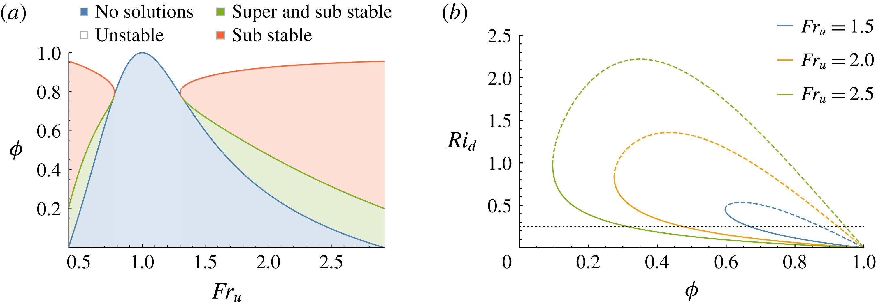
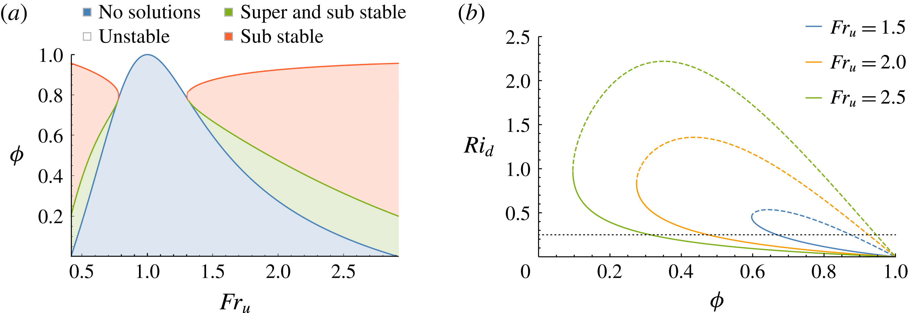
is illustrated by the shaded blue region of the regime diagram in figure 3(a). The roots of (4.6) require that
 $0.417\leqslant Fr_{u}\leqslant 2.921$
, otherwise the model predicts
 $\unicode[STIX]{x1D719}<0$
, which is unphysical. Outside of this range, the flow has sufficient momentum (or equivalently small enough buoyancy) that all the fluid in the current can become modified through mixing, and in § 5 we present a further series of solutions for that case.
These figures refer to the case with a lower uniform region overlain by an interfacial linearly stratified mixing region. (a) A regime diagram illustrating the nature of solutions for an upstream Froude number
 $Fr_{u}$
and downstream uniform flow fraction
 $\unicode[STIX]{x1D719}$
. Blue shaded areas are regions of no solution due to violation of conservation laws. Green shaded areas are where
 $Ri_{d}\geqslant 1/4$
and the downstream flow is stable for both supercritical and subcritical solutions. Red shaded areas are stable for subcritical solutions and unstable for supercritical solutions. White areas are where
 $Ri_{d}<1/4$
and the downstream flow is unstable for all solutions. (b) The variation of downstream gradient Richardson number with uniform flow fraction
 $\unicode[STIX]{x1D719}$
. Supercritical solutions are shown as solid lines and subcritical solutions as dashed lines. The two solution branches converge when
 $\unicode[STIX]{x1D719}=\unicode[STIX]{x1D719}_{min}$
at
 $Ri_{d}(\unicode[STIX]{x1D719}_{min})$
. The turning point of the subcritical branch gives a maximal downstream gradient Richardson number
 $Ri_{d_{max}}$
for each upstream Froude number
 $Fr_{u}$
. Portions of both branches below the black dotted line
 $Ri_{d}=1/4$
are unstable.
Furthermore, we note that the equations for the conservation of buoyancy and momentum lead to an equation which is cubic in nature with three real roots. One of these roots is unphysical since it requires
 $h_{d}<0$
. However, the two remaining roots may be interpreted physically. One root, which we will denote supercritical by analogy with § 3, can be thought of as evolving continuously away from the upstream uniform flow by turbulent entrainment. The entrainment gradually erodes the interface, creating a deepening interfacial mixing layer. The other root, which we will denote subcritical, can be interpreted as the case in which the fluid undergoes a discontinuous hydraulic jump to a conjugate flow state where the local Froude number
 ${<}1$
. This could possibly occur after a period of supercritical interfacial entrainment.
We can also determine which of the family of solutions, that are consistent with momentum and buoyancy conservation, are stable. This is done by determining those solutions for which the gradient Richardson number
 $Ri_{d}\geqslant 0.25$
for both supercritical and subcritical branches. The case for which both supercritical and subcritical branches are stable is shaded green in figure 3(a). The red shaded area indicates where only the subcritical solution branch is stable and the supercritical unstable. We note that transition to a uniform flow downstream (
 $\unicode[STIX]{x1D719}=1$
) is always unstable in that the gradient Richardson number tends to zero as the mixed layer thickness tends to zero, with a non-zero jump in density and velocity across the layer.
In figure 3(b) we illustrate the variation of the downstream gradient Richardson number
 $Ri_{d}$
as a function of the fractional depth of the well-mixed lower region of the flow
 $\unicode[STIX]{x1D719}$
for a series of upstream Froude numbers
 $Fr_{u}$
. The supercritical branch, denoted with solid lines, converges to the subcritical solution branch, denoted with dashed lines, at the value
 $Ri_{d}(Fr_{u},\unicode[STIX]{x1D719}_{min})$
. The dotted black line indicates
 $Ri_{d}=1/4$
, below which all downstream flows are unstable.
4.2 Entrainment
We can express the dimensionless flux of entrained ambient fluid associated with the transition from the upstream uniform flow to the downstream structured flow in terms of the expression
 $$\begin{eqnarray}\unicode[STIX]{x0394}Q=\frac{\hat{u} {\hat{h}}(1+\unicode[STIX]{x1D719})}{2}-1=\frac{1-\unicode[STIX]{x1D719}}{2(1+2\unicode[STIX]{x1D719})}.\end{eqnarray}$$
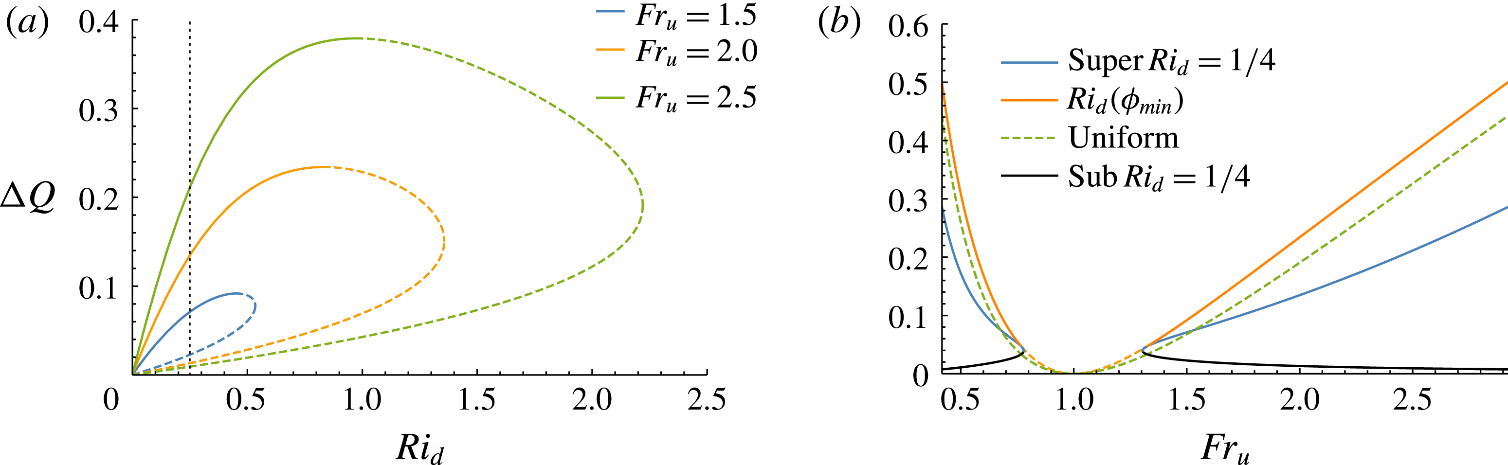
In figure 4(a) we plot the variation of the dimensionless entrainment flux
 $\unicode[STIX]{x0394}Q$
as a function of the downstream gradient Richardson number, for three fixed values of the upstream Froude number
 $Fr_{u}$
. We note that flows with downstream gradient Richardson number
 $Ri_{d}\geqslant 1/4$
are stable to downstream disturbances of any wavenumber (Turner Reference Turner1979); and for portions of the curve with
 $Ri_{d}<1/4$
the solutions are unstable. Solutions from the supercritical branch are denoted with solid lines, and solutions from the subcritical branch are denoted with dashed lines. The maximal mixing solution occurs at the convergence of the two branches, with the gradient Richardson number associated with
 $\unicode[STIX]{x1D719}_{min}$
.
These figures refer to the case with a lower uniform region overlain by an interfacial linearly stratified mixing region. (a) Dimensionless entrainment flux as a function of the downstream gradient Richardson number for a fixed upstream Froude number
 $Fr_{u}$
. Supercritical branch solutions are shown as solid lines and subcritical as dashed lines. Maximal entrainment occurs at the convergence of the two branches
 $\unicode[STIX]{x1D719}_{min}$
. Points of the curve left of the line
 $Ri_{d}=1/4$
are unstable. (b) The downstream dimensionless entrainment flux
 $\unicode[STIX]{x0394}Q$
as a function of upstream inflow Froude number
 $Fr_{u}$
for
 $Ri_{d}(\unicode[STIX]{x1D719}_{min})$
in orange, the supercritical solution branch with gradient Richardson number
 $Ri_{d}=1/4$
in blue, the subcritical solution branch with gradient Richardson number
 $Ri_{d}=1/4$
in black, and the uniform downstream calculation of § 3 in green. The dashed portions of the curves illustrate where the downstream flow is unstable.

In figure 4(b) we compare the flux of entrained fluid predicted for the reference solutions in which we assume the flow downstream is uniform (dashed green line; see § 3 (3.7)) and that predicted by the solutions which have a linearly stratified mixed layer downstream. Curves are shown for the solutions in which: (i) the supercritical branch’s gradient Richardson number is
 $Ri_{d}=0.25$
(blue line), (ii) the subcritical branch has
 $Ri_{d}=1/4$
(black line), and (iii) for the solutions which have the maximal mixing and
 $Ri_{d}(\unicode[STIX]{x1D719}_{min})$
(orange line). The dashed portions of the orange line illustrate where the gradient Richardson number of the downstream flow with maximal mixing is unstable (ie.
 $Ri_{d}(\unicode[STIX]{x1D719}_{min})<0.25$
). It is seen that the model in which we assume the flow is uniform downstream (§ 3) leads to less mixing than the stratified flow solutions with largest possible downstream gradient Richardson number. However, we can also see that stratified flows with
 $Ri_{d}=1/4$
have smaller total flux of entrained fluid than these reference uniform flow solutions. Furthermore, the amount of fluid entrained by the subcritical branch with
 $Ri_{d}=1/4$
is less than the supercritical branch. The model also shows that there is a region
 $0.770\leqslant Fr_{u}\leqslant 1.319$
where no downstream flows are stable.
4.3 Energetics – supercritical and subcritical branches
A clear way to illustrate the difference between the two solution branches is to consider the energy dissipation
 $\unicode[STIX]{x0394}E(Fr_{u},\unicode[STIX]{x1D719})$
across the transition. The steady energy flux lost per unit distance through the transition is given by
 $$\begin{eqnarray}\frac{\unicode[STIX]{x2202}}{\unicode[STIX]{x2202}x}\left(\int _{0}^{h}u\left(\frac{u^{2}}{2}+g^{\prime }y\right)\,\text{d}y+\int _{0}^{h}u\left(\int _{y}^{h}g^{\prime }\,\text{d}y^{\ast }\right)\text{d}y\right)=\frac{\unicode[STIX]{x2202}(\unicode[STIX]{x0394}E)}{\unicode[STIX]{x2202}x},\end{eqnarray}$$
where the first term inside the differential corresponds to the flux of specific energy (kinetic and potential) and second term corresponds to the flux of the vertical integral of hydrostatic pressure (internal energy). Substituting the model solution allows us to write the dissipation as
 $$\begin{eqnarray}\unicode[STIX]{x0394}\hat{E}=\frac{Fr_{u}^{3}}{2}+Fr_{u}-\frac{{\hat{h}}^{5/2}}{24}\left(\frac{1-\unicode[STIX]{x1D719}}{Ri_{d}}\right)^{1/2}\left(\frac{3(1-\unicode[STIX]{x1D719})(1+3\unicode[STIX]{x1D719})}{Ri_{d}}+5+10\unicode[STIX]{x1D719}+9\unicode[STIX]{x1D719}^{2}\right),\end{eqnarray}$$
where
 $\unicode[STIX]{x0394}\hat{E}=\unicode[STIX]{x0394}E/g_{u}^{\prime 3/2}h_{u}^{5/2}$
. As was noted in § 3, for a uniform flow, there are two conjugate solutions with no mixing, by analogy with classical hydraulics. We expect a similar result in the present case. The first solution with zero entrainment corresponds to the solution where no transition occurs, and has
 $\unicode[STIX]{x0394}E=0$
. Whilst the conjugate zero-entrainment solution, involving a hydraulic jump, has a finite dissipation when
 $\unicode[STIX]{x1D719}=1$
(in equivalence with figure 2
b). For a fixed source Froude number
 $Fr_{u}=2$
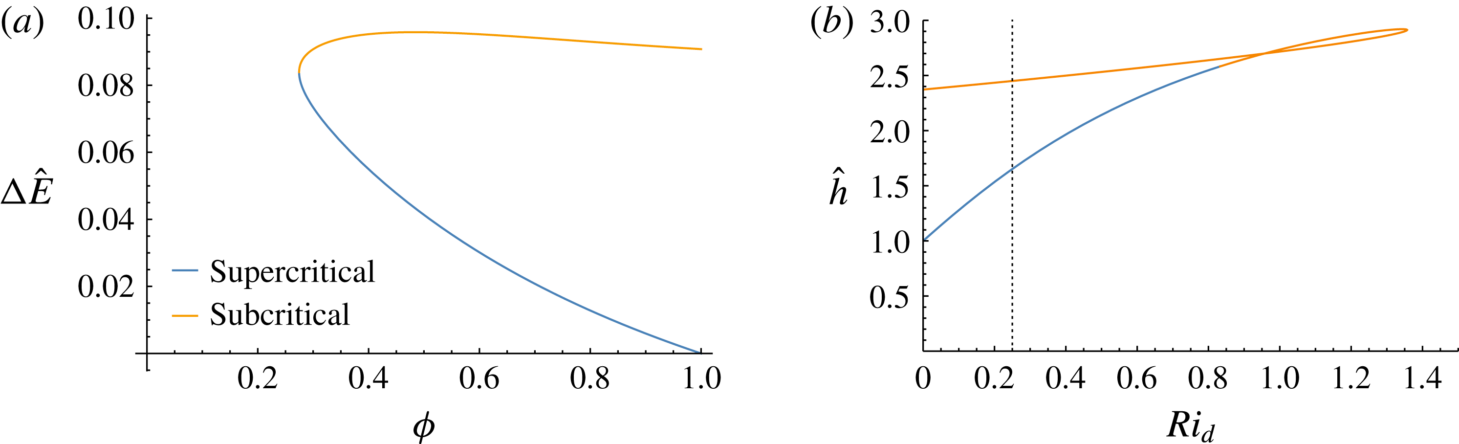
, figure 5(a) illustrates the energy dissipation as
 $\unicode[STIX]{x1D719}$
varies. On the supercritical branch the dissipation is 0 at
 $\unicode[STIX]{x1D719}=1$
. As
 $\unicode[STIX]{x1D719}$
is then decreased, which corresponds to an increase in the thickness of the stratified zone, a finite amount of energy is dissipated. However, even when
 $\unicode[STIX]{x1D719}=1$
, the energy dissipation on the subcritical branch is finite. As
 $\unicode[STIX]{x1D719}$
then decreases, corresponding to progressively more mixing, the energy dissipation increases to a maximum value of 0.096 when
 $\unicode[STIX]{x1D719}=0.484$
, which corresponds to a gradient Richardson number
 $Ri_{d}=1.337$
. The energy dissipation then falls as the solution converges towards the supercritical branch with
 $\unicode[STIX]{x1D719}_{min}=0.275$
. It is unphysical for the dissipation to fall via the process of entrainment, so solutions along the subcritical branch are restricted to values of
 $\unicode[STIX]{x1D719}>0.484$
. Solutions in the range
 $\unicode[STIX]{x1D719}_{min}<\unicode[STIX]{x1D719}<0.484$
may be accessed through a discontinuous hydraulic jump from the supercritical branch.
In figure 5(b) we show how the non-dimensional downstream height
 ${\hat{h}}$
varies as a function of the downstream gradient Richardson number
 $Ri_{d}$
for both supercritical and subcritical solution branches. In this figure we can see that the supercritical branch moves continuously away from 1 by the process of interfacial entrainment, which deepens the interfacial mixing zone and increases the gradient Richardson number to the value at
 $Ri_{d}(\unicode[STIX]{x1D719}_{min})$
. However for subcritical solutions the discontinuous nature of the change in height can be seen, with the special zero-entrainment case jumping to a height
 ${\hat{h}}=2.375$
. Entrainment can then continuously occur along the subcritical solution branch until
 $Ri_{d}=1.337$
is reached and the maximal energy has been dissipated. Other heights could be reached beyond this value, but via a discontinuous process after which evolution would be restricted in order that the energy continues to dissipate through mixing.
These figures refer to the case with a lower uniform region overlain by an interfacial linearly stratified mixing region. (a) The variation of dimensionless energy dissipation
 $\unicode[STIX]{x0394}\hat{E}$
with the downstream uniform flow fraction
 $\unicode[STIX]{x1D719}$
for a fixed upstream Froude number
 $Fr_{u}=2$
. The blue line corresponds to the supercritical branch, which continuously moves away from the
 $\unicode[STIX]{x1D719}=1$
solution where no transition occurs. The orange line corresponds to the subcritical branch, which has finite dissipation at
 $\unicode[STIX]{x1D719}=1$
corresponding to a hydraulic jump with no entrainment. This discontinuous transition can then dissipate more energy as a shear layer is created by the entrainment of fluid up to a maximum value
 $\unicode[STIX]{x0394}\hat{E}=0.096$
. (b) The variation of dimensionless downstream height
 ${\hat{h}}$
with downstream gradient Richardson number
 $Ri_{d}$
for a fixed upstream Froude number
 $Fr_{u}=2$
. Solutions to the left of the black dotted line
 $Ri_{d}=1/4$
are unstable.

5 Fully modified layer
$Fr>2.921$

For flows where the upstream Froude number
 $Fr_{u}=2.921$
, the entire flow can become linearly stratified with
 $\unicode[STIX]{x1D719}=0$
, and the buoyancy at the base just equal to the initial buoyancy upstream. For upstream Froude numbers larger than this critical value, further mixing may arise, and this can lead to further dilution of the flow, with the buoyancy at the base of the current
 $g_{d}^{\prime }$
falling below the original value of the upstream flow
 $g_{u}^{\prime }$
. Now, in this case, the downstream velocity and buoyancy profiles have the form
 $$\begin{eqnarray}\displaystyle & \displaystyle u(x_{d},y)=\frac{u_{d}(h_{d}-y)}{h_{d}},\quad g^{\prime }(x_{d},y)=\frac{g_{d}^{\prime }(h_{d}-y)}{h_{d}}. & \displaystyle\end{eqnarray}$$
By substituting into (2.2) we find the shape factors
 $S_{1}=1/2$
,
 $S_{3}=1/6$
,
 $S_{2}=S_{4}=1/3$
and the following (dimensional) relation with the uniform flow at the source
 $x=0$
 $$\begin{eqnarray}\displaystyle u_{u}g_{u}^{\prime }h_{u} & = & \displaystyle {\textstyle \frac{1}{3}}u_{d}g_{d}^{\prime }h_{d},\end{eqnarray}$$
 $$\begin{eqnarray}\displaystyle u_{u}^{2}h_{u}+{\textstyle \frac{1}{2}}g_{u}^{\prime }h_{u}^{2} & = & \displaystyle {\textstyle \frac{1}{3}}u_{d}^{2}h_{d}+{\textstyle \frac{1}{6}}g_{d}^{\prime }h_{d}^{2}.\end{eqnarray}$$
 $Ri_{d}=g_{d}^{\prime }h_{d}/u_{d}^{2}$
,
 $Fr_{u}$
,
 $\hat{u} =u_{d}/u_{u}$
,
 ${\hat{g}}^{\prime }=g_{d}^{\prime }/g_{u}^{\prime }$
and
 ${\hat{h}}=h_{d}/h_{u}$
as
 $$\begin{eqnarray}\displaystyle Fr_{u} & = & \displaystyle \displaystyle \frac{\left({\hat{g}}^{\prime }{\hat{h}}\right)^{3/2}}{3Ri_{d}^{1/2}},\end{eqnarray}$$
 $$\begin{eqnarray}\displaystyle \displaystyle Fr_{u}^{2}+\frac{1}{2} & = & \displaystyle \displaystyle \frac{{\hat{g}}^{\prime }{\hat{h}}^{2}}{3}\left(\frac{1}{Ri_{d}}+\frac{1}{2}\right),\end{eqnarray}$$
 $$\begin{eqnarray}\displaystyle \hat{u} =\frac{3^{1/3}}{Fr_{u}^{2/3}Ri_{d}^{1/3}},\quad {\hat{g}}^{\prime }=\frac{3^{1/3}Fr_{u}^{4/3}(Ri_{d}+2)}{(2Fr_{u}^{2}+1)Ri_{d}^{1/3}},\quad {\hat{h}}=\frac{3^{1/3}(2Fr_{u}^{2}+1)Ri_{d}^{2/3}}{Fr_{u}^{2/3}(Ri_{d}+2)}. & & \displaystyle\end{eqnarray}$$
The dimensionless entrainment flux in this case is given by
 $$\begin{eqnarray}\unicode[STIX]{x0394}Q=\frac{3^{2/3}(1+2Fr_{u}^{2})Ri_{d}^{1/3}}{2Fr_{u}^{4/3}(Ri_{d}+2)}-1.\end{eqnarray}$$
In figure 6(b) we have plotted the mixing associated with downstream gradient Richardson number
 $Ri_{d}$
. The maximal mixing in this case occurs at
 $Ri_{d}=1$
, which is given by
 $$\begin{eqnarray}\unicode[STIX]{x0394}Q_{max}=\frac{1+2Fr_{u}^{2}}{24^{1/3}Fr_{u}^{4/3}}-1.\end{eqnarray}$$
Similarly the energy dissipation due to a transition to an entirely linearly stratified state is given by substituting the model (5.1) into (4.8), then expressing the result in dimensionless form we obtain
 $$\begin{eqnarray}\unicode[STIX]{x0394}\hat{E}=\frac{Fr_{u}^{3}}{2}+Fr_{u}-\frac{{\hat{g}}^{3/2}{\hat{h}}^{5/2}}{24}\left(\frac{3}{Ri_{d}^{3/2}}+\frac{5}{Ri_{d}^{1/2}}\right).\end{eqnarray}$$
The smallest value of
 $g_{d}^{\prime }$
that the flow can attain is given by
 $$\begin{eqnarray}g_{d_{min}}^{\prime }=\frac{81^{1/3}Fr_{u}^{4/3}}{1+2Fr_{u}^{2}}.\end{eqnarray}$$
Any buoyancy
 $g_{d}^{\prime }$
at the base of the downstream flow smaller than this value violates conservation of momentum and buoyancy. The range of validity for solutions with the entire layer fully modified
 $Fr_{u}>2.921$
is complementary to the range of validity for the solutions with an interfacial mixing layer overlying a uniform layer as given in § 4. Theoretically, in the case
 $0.471\leqslant Fr_{u}\leqslant 2.921$
, one can find a solution with
 $\unicode[STIX]{x1D719}=0$
for which
 $g_{d}^{\prime }>g_{u}^{\prime }$
; however, this is unphysical since the fluid cannot become more concentrated as it migrates downstream.
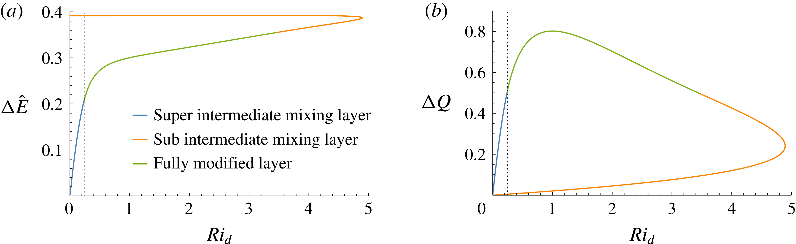
These figures refer to the case when the flow is fully modified and is linearly stratified throughout. (a) A diagram illustrating the variation of dimensionless energy dissipation
 $\unicode[STIX]{x0394}\hat{E}$
with downstream gradient Richardson number
 $Ri_{d}$
for a fixed upstream Froude number
 $Fr_{u}=4$
. The orange curve illustrates solutions from the subcritical interfacial mixing layer model, the blue curve illustrates solutions from the supercritical interfacial mixing layer model, and the green curve illustrates solutions from the fully modified layer model. Solutions to the left of the black dotted line
 $Ri_{d}=1/4$
are unstable. (b) The downstream entrainment flux
 $\unicode[STIX]{x0394}Q$
as a function of downstream gradient Richardson number
 $Ri_{d}$
for a fixed upstream inflow Froude number
 $Fr_{u}=4$
. The orange curve illustrates solutions from the subcritical interfacial mixing layer model, the blue curve illustrates solutions from the supercritical interfacial mixing layer model, and the green curve illustrates solutions from the fully modified layer model. Note that solutions to the left of the line
 $Ri_{d}=1/4$
are unstable.

To illustrate the complementary nature of the two regimes
 $0.471\leqslant Fr_{u}\leqslant 2.921$
(interfacial mixing layer) and
 $Fr_{u}>2.921$
(fully modified) we fix an upstream Froude number
 $Fr_{u}=4$
. From the intermediate interfacial mixing layer model we have that
 $0\leqslant \unicode[STIX]{x1D719}\leqslant 1$
for
 $0\leqslant Ri_{d}\leqslant 0.240$
on the supercritical branch. Similarly, for the subcritical branch we have two values of
 $\unicode[STIX]{x1D719}$
for gradient Richardson number in the range
 $3.439\leqslant Ri_{d}\leqslant Ri_{d_{max}}$
and a single value of
 $\unicode[STIX]{x1D719}$
for the range
 $0\leqslant Ri_{d}\leqslant 3.439$
. For the fully modified layer model the range
 $0.240\leqslant Ri_{d}\leqslant 3.493$
gives
 ${\hat{g}}^{\prime }\leqslant 1$
, and outside of this range the solution requires the unphysical case
 ${\hat{g}}^{\prime }>1$
. Hence we can see in figure 6(a,b) how the energy dissipation
 $\hat{E}$
and entrainment flux
 $\unicode[STIX]{x0394}Q$
vary as a function of the downstream gradient Richardson number. Since the Froude number is larger than the critical value 2.921 the convergence of the two solution branches is broken and the subcritical and supercritical branches are separated in gradient Richardson number space. However, by allowing the buoyancy at base of the flow to decrease from its initial value, the model solutions in which the current is fully stratified continuously join these distinct branches.
6 Discussion
In this paper we have explored the mixing which occurs when an initially uniform and dense fluid flows along a horizontal boundary beneath a second fluid of smaller density. We use an ansatz for the structure of the downstream flow which includes a region of uniform shear with a linear density gradient above a region of uniform flow and density, and constrain the properties of this flow using the conservation of momentum and buoyancy. When the stratified zone has a gradient Richardson number in excess of 1/4, the flow is stable, and we show that the volume of entrained ambient fluid in this flow increases with the upstream Froude number. We also calculate the solution which has the maximum entrainment of ambient fluid, which again has an increasing entrainment flux with upstream Froude number. For upstream Froude numbers in excess of 2.921 the stratified zone may extend to the lower boundary of the domain, so that there is no uniform region of flow.
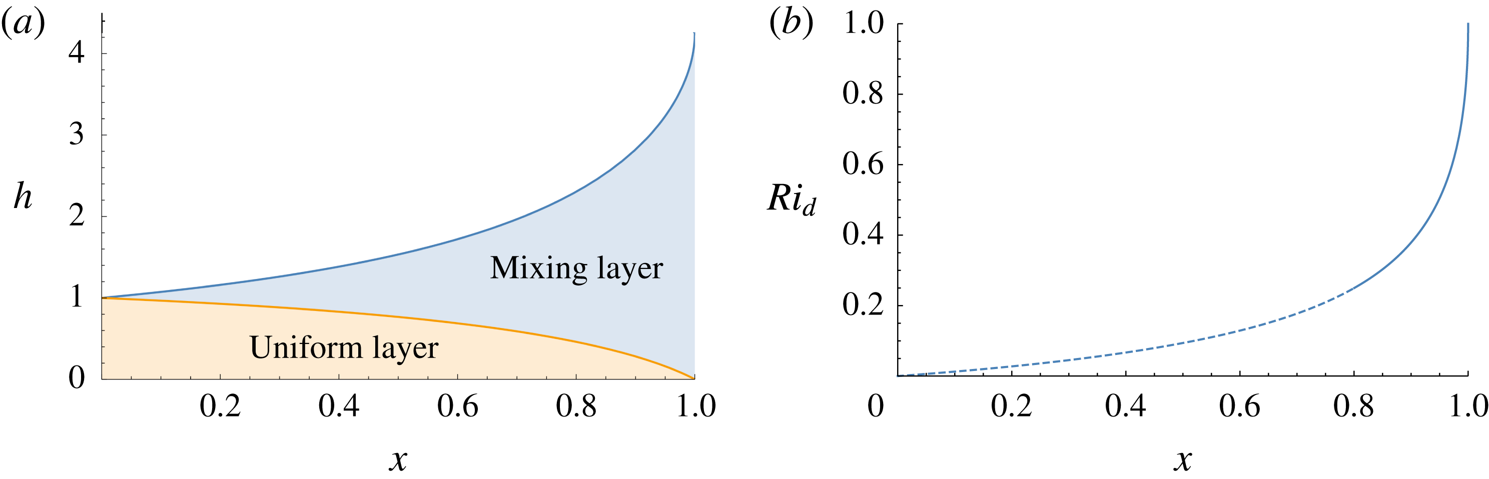
(a) The spacelike evolution of the supercritical solution branch’s interfacial mixing layer in blue, and the uniform layer in orange, for the critical upstream Froude number
 $Fr=2.921$
. (b) The evolution of the downstream gradient Richardson number in space. The dashed line illustrates where the curve is unstable, and a solid line illustrates where the curve is stable. For convenience in both figures the length scale is chosen such that the spacelike co-ordinate
 $x$
varies between 0 and 1. This corresponds to a theoretical constant entrainment coefficient
 $\unicode[STIX]{x1D700}_{0}\approx 0.52$
from (2.3).

In figure 7(a), we illustrate the variation of the depth of the supercritical solution and of the stratified zone for a flow which has an upstream Froude number of 2.921. In figure 7(b), we illustrate the gradient Richardson number corresponding to each of these downstream solutions. Those solutions for which
 $Ri_{d}>1/4$
are stable and shown with a solid line. Using (2.3a
) we can calculate an adjustment length scale as a function of
 $\unicode[STIX]{x1D700}$
. Figure 7(a,b) illustrate the shape of the transition zone with
 $x$
, which for convenience has been scaled to vary from 0 to 1. This corresponds to a theoretical constant entrainment coefficient
 $\unicode[STIX]{x1D700}_{0}\approx 0.52$
. If the actual entrainment coefficient is
 $\unicode[STIX]{x1D700}$
the adjustment length is given by
 $L\sim \unicode[STIX]{x1D700}_{0}/\unicode[STIX]{x1D700}$
.
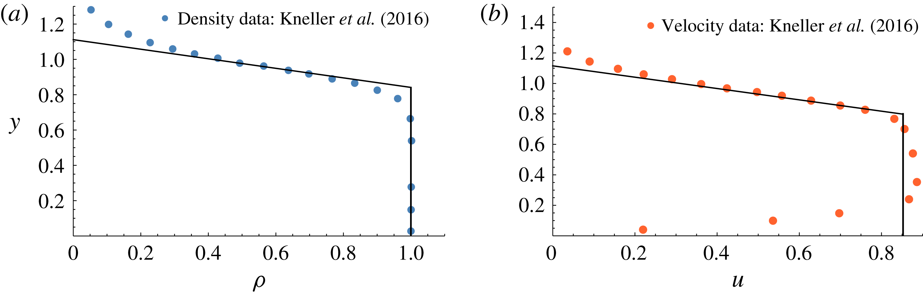
(a) Density profile data from the numerical simulation of a gravity current on a horizontal boundary presented by Kneller et al. (Reference Kneller, Nasr-Azadani, Radhakrishnan and Meiburg2016). The black line overlain shows the profile as calculated by the model in § 4 for an upstream Froude number
 $Fr_{u}=0.67$
. (b) Velocity profile data, again taken from Kneller et al. (Reference Kneller, Nasr-Azadani, Radhakrishnan and Meiburg2016). We note that this Froude number,
 $Fr_{u}=0.67$
, corresponds to the flow which conserves momentum flux, and has a momentum flux equal to the downstream momentum flux as calculated from the data presented by Kneller et al. (Reference Kneller, Nasr-Azadani, Radhakrishnan and Meiburg2016) and shown in both panels. The numerical solutions of Kneller et al. (Reference Kneller, Nasr-Azadani, Radhakrishnan and Meiburg2016) include some bottom drag, and therefore lose some momentum, so that the source Froude number in their calculations is in fact
 $Fr=0.78$
.

We now compare the predictions of our model with the numerical simulations of gravity currents as reported by Kneller et al. (Reference Kneller, Nasr-Azadani, Radhakrishnan and Meiburg2016). For example, in figure 8 we present density and velocity data taken from figure 2(a) of Kneller et al. (Reference Kneller, Nasr-Azadani, Radhakrishnan and Meiburg2016). This data corresponds a gravity current travelling along a horizontal bottom boundary. Note, in their calculation the buoyancy is associated with dense particles, which are assumed to have zero settling velocity, and hence their simulation is equivalent to a saline gravity current as explored in this paper. However, in their simulation the effect of momentum loss due bottom friction is included. To make our results directly comparable to that of Kneller et al. (Reference Kneller, Nasr-Azadani, Radhakrishnan and Meiburg2016) we need to account for the momentum loss not captured by our inviscid approximation. To do this we use the momentum flux, as calculated from the transect of velocity and density profiles in the numerical data figure 8, to define an equivalent inlet condition for our model. In this case our model current, which conserves momentum, has value
 $Fr_{u}=0.67$
. This is smaller than the source Froude number quoted by Kneller et al. (Reference Kneller, Nasr-Azadani, Radhakrishnan and Meiburg2016) of
 $Fr=0.78$
. In figure 8 we overlay the predictions of our model with the numerical data, setting
 $Fr_{u}=0.67$
for momentum conservation and choosing
 $\unicode[STIX]{x1D719}=0.75$
as a best fit. This implies a stable gradient Richardson number
 $Ri_{d}=0.59$
in the interfacial mixing layer. We do note the small discrepancies at the two ends of the linearly stratified upper portion arise from the action of diffusion in the TURBINS code used by Kneller et al. (Reference Kneller, Nasr-Azadani, Radhakrishnan and Meiburg2016). We have also analysed some further numerical simulations presented in figure 7(d,e,f) of Hogg et al. (Reference Hogg, Nasr-Azadani, Ungarish and Meiburg2016). We find that the vertical density profiles at a distance 10 units behind the head in each of their figures can also be accurately represented by a linearly stratified layer overlying a more uniform layer, which is consistent with our ansatz.
It is also of interest to note that our model predicts that the flow entrains a volume flux between 0.1–0.5 of the source flux with upstream Froude numbers in the range 1.5–3 (figure 4 b). The exact entrainment rate depends on the downstream gradient Richardson number of the flow. These predictions are similar in magnitude to the recent experimental data reported by Sher & Woods (Reference Sher and Woods2017), who found the entrainment flux into a horizontal dense jet entering a channel of less dense fluid was in the range 0.34–0.63 for a comparable range of upstream Froude numbers; although we note that the velocity and buoyancy profiles they report were somewhat more complex than the idealised model presented herein. The present calculations illustrate how important the inflow mixing zone may be in the development of stratification and establishment of a flow with a gradient Richardson number greater than 1/4 as a turbulent gravity current develops. This can have very significant implications for the subsequent entrainment of ambient into such a current.
As well as the continuous erosion of the interface of a supercritical flow, a hydraulic jump may lead to a subcritical flow downstream, beyond which the evolution may continue through gradual erosion and mixing across the interface. A hydraulic jump may involve a discontinuous jump to any of the possible downstream gradient Richardson numbers; however, the subsequent erosion of the interface after a jump is restricted to the maximum dissipation solution in order that the overall energy of the flow does not increase downstream, which would be unphysical.
A key feature of the model solutions is that the gradient Richardson number is restricted to values in excess of 1/4, so that the downstream flows are stable. This restriction, coupled with the ansatz of a linear stratification, leads to the prediction of less mixing than is possible if the downstream flow has vertically uniform velocity and buoyancy. This suggests that the structure of the flow is key in constraining the mixing. In depth-averaged models, this structure is expressed in terms of shape factors: the present solutions correspond to the family of such solutions in which the vertical structure of the flow involves an interfacial mixing zone with linear stratification and a lower uniform region, in which the buoyancy corresponds to the original buoyancy of the upstream flow.
The present analysis, although simplified, identifies the importance of constraining the structure and mixing in such flows, with either new laboratory experiments and direct numerical solutions. Nonetheless, even with the idealised structure of the flow, the present study provides insight and some constraints on the process of mixing as a steady gravity current becomes established downstream of a source of dense fluid.