1 Introduction
In spite of the great advances in computational fluid dynamics, the analytical results from linear unsteady potential theory are still widely used to estimate aerodynamic forces of flapping thin airfoils. This is particularly the case, of course, for large Reynolds number and small amplitude of the oscillations, where the linear potential theory of Theodorsen (Reference Theodorsen1935) and von Kármán & Sears (Reference von Kármán and Sears1938) is quite accurate in predicting the unsteady lift force (Baik et al.
Reference Baik, Bernal, Granlund and Ol2012; Mackowski & Williamson Reference Mackowski and Williamson2015, Reference Mackowski and Williamson2017; Cordes et al.
Reference Cordes, Kampers, Meissner, Tropea, Pinke and Hölling2017). The thrust force of an oscillating airfoil within the linear theory of Theodorsen was computed by Garrick (Reference Garrick1936), among others (see e.g. Sedov Reference Sedov1965), following the ideas of von Kármán & Burgers (Reference von Kármán, Burgers and Durand1935). This formulation was subsequently used by Lighthill (Reference Lighthill1970) and Wu (Reference Wu1971) to analyse the optimum configuration that maximizes the propulsive efficiency of the oscillating airfoil. These authors, who also considered the more general case of flexible airfoils, found, for instance, that the efficiency is maximized when pitch lags heave by
 $90^{\circ }$
in the flapping cycle, in qualitative agreement with experimental results. However, the predictions about the optimum values for maximum propulsive efficiency of the other parameters, such as the reduced frequency, the axis of pitch or the ratio between pitch and heave amplitudes, were either not conclusive enough or in clear disagreement with later numerical results from the full Navier–Stokes equations and with experimental data (Anderson et al.
Reference Anderson, Streitlien, Barret and Triantafyllou1998; Isogai, Shinmoto & Watanabe Reference Isogai, Shinmoto and Watanabe1999; Jones & Platzer Reference Jones and Platzer1999; Tuncer & Kaya Reference Tuncer and Kaya2005; Heathcote & Gursul Reference Heathcote and Gursul2007; Young & Lai Reference Young and Lai2007; Quinn, Lauder & Smits Reference Quinn, Lauder and Smits2015; Mackowski & Williamson Reference Mackowski and Williamson2015, Reference Mackowski and Williamson2017; Das, Shukla & Govardhan Reference Das, Shukla and Govardhan2016). This disagreement persists even for small amplitude of the oscillations, when the vortex wake behind the airfoil is almost flat and the leading-edge separation effects are very weak.
The thrust force has been recently obtained from the general vortical impulse theory within the same framework of linear potential theory (Fernandez-Feria Reference Fernandez-Feria2016, hereafter F-F for short), correcting Garrick’s (Reference Garrick1936) result, especially for reduced frequencies larger than approximately unity. Garrick’s thrust force takes into account the effect of the leading-edge suction and the projection in the flight direction of the pressure force on the airfoil, while the vortical impulse theory considers the whole effect of the vorticity distribution on the airfoil, not only at the leading edge. As a consequence, the propulsive efficiency resulting from the impulse theory decays as
 $k^{-1}$
for large reduced frequency
 $k$
, in agreement with experimental and numerical results (see F-F), and in contrast to Garrick’s propulsive efficiency, which tends to a constant (
 $1/2$
) for large
 $k$
for any flapping condition.
However, for small
 $k$
, the thrust coefficient and the propulsive efficiency from the two approaches are quite similar, and disagree with experimental and numerical results, even for very small magnitudes of the pitching and heaving amplitudes. This disagreement is obviously due to the fact that potential theory does not take into account the viscous drag on the airfoil, which is most important for small reduced frequencies where the absolute value of the time-averaged thrust coefficient
 $|C_{T}|$
from the linear potential theory is very small (
 $|C_{T}|\rightarrow 0$
as
 $k\rightarrow 0$
). This problem can be fixed in a relatively easy way, however, by adding a quasi-static averaged thrust of the airfoil section,
 $C_{T0}$
, to the theoretical
 $C_{T}$
(Mackowski & Williamson Reference Mackowski and Williamson2015, Reference Mackowski and Williamson2017). It was shown in F-F that the addition of this constant
 $C_{T0}$
to the time-averaged thrust coefficient obtained from the vortical impulse theory fitted quite well to the experimental results of Mackowski & Williamson (Reference Mackowski and Williamson2015), much better than with Garrick’s (Reference Garrick1936) thrust with the same constant offset. As we shall see in § 2, the improvement in the resulting propulsive efficiency by adding this
 $C_{T0}$
is even better, showing a remarkable agreement with experimental data, while the propulsive efficiency of Garrick with the same constant quasi-static thrust
 $C_{T0}$
shows a poorer agreement.
The main problem with this constant quasi-static thrust is that it obviously has to be obtained externally to the linear potential theory, either from experimental data or from numerical simulations with the full Navier–Stokes equations. We shall see, however, that the propulsive efficiency from the corrected linearized potential theory with the addition of a reasonable constant value of
 $C_{T0}$
is so improved, for both small and large reduced frequencies, that it becomes a powerful analytical tool for estimating the optimum conditions that maximize propulsive efficiency for heaving and pitching two-dimensional and thin airfoils at small amplitudes.
This objective of the present work, and its main contribution in relation to F-F, is to use this improved formulation to map the dynamics of the foil over a large range of parameters and to explore the conditions associated with optimal aerodynamic performance. This analysis may have some implications for the design of flapping-wing vehicles (Platzer et al. Reference Platzer, Jones, Young and Lai2008).
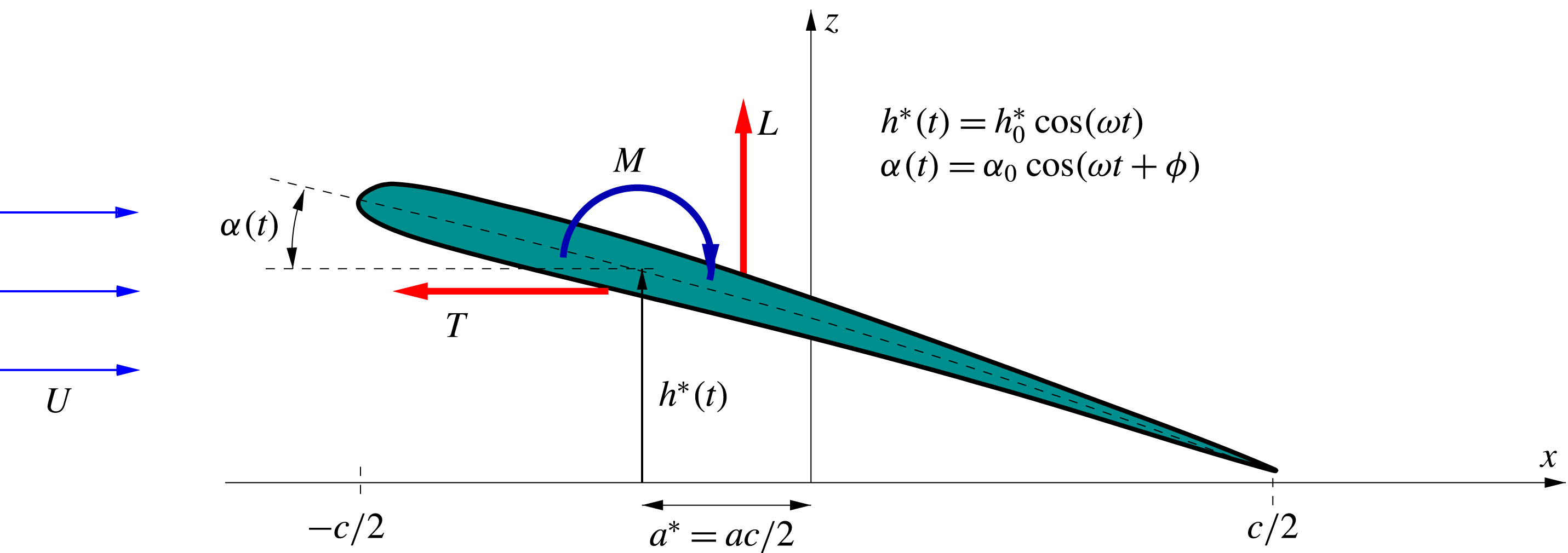
Sketch of the kinematics of the pitching and heaving airfoil. The non-dimensional pivot point parameter
 $a$
is
 $-1$
for a pivot location at the leading edge and
 $+1$
at the trailing edge.

2 Thrust and efficiency expressions and their comparison with experimental data
The thrust coefficient computed from the linear potential theory for a heaving and pitching two-dimensional airfoil oscillating sinusoidally with frequency
 $\unicode[STIX]{x1D714}$
and with average forward velocity
 $U$
(see figure 1) can be formally written as (Garrick Reference Garrick1936; Fernandez-Feria Reference Fernandez-Feria2016)
 $$\begin{eqnarray}C_{T}\equiv \frac{T}{\frac{1}{2}\unicode[STIX]{x1D70C}U^{2}c}=t_{h}(k)(kh_{0})^{2}+t_{a}(k,a)\unicode[STIX]{x1D6FC}_{0}^{2}+t_{ha}(k,a,\unicode[STIX]{x1D719})\unicode[STIX]{x1D6FC}_{0}kh_{0},\end{eqnarray}$$
where
 $T$
is the (time-averaged) thrust force per unit span and
 $c$
the chord length of the airfoil. In this expression,
 $h_{0}=2h_{0}^{\ast }/c$
is the heave amplitude
 $h_{0}^{\ast }$
scaled with the half-chord,
 $\unicode[STIX]{x1D6FC}_{0}$
is the pitch amplitude,
 $t_{h}$
is a function of the reduced frequency,
 $$\begin{eqnarray}k=\frac{c\unicode[STIX]{x1D714}}{2U},\end{eqnarray}$$
 $t_{a}$
is a function of
 $k$
and
 $a=2a^{\ast }/c$
, or location of the pitch axis
 $a^{\ast }$
(in relation to the centre of the airfoil) scaled with the half-chord, and
 $t_{ha}$
is a function of
 $k$
,
 $a$
and the phase shift
 $\unicode[STIX]{x1D719}$
between pitching and heaving motions. These functions
 $t_{h}$
,
 $t_{a}$
and
 $t_{ha}$
are summarized in appendix A according to Garrick (Reference Garrick1936) and from the vortical impulse theory (F-F). For pure heaving motion the last two terms in (2.1) vanish, so that the thrust coefficient depends only on
 $k$
and
 $h_{0}$
, while for a pure pitching motion just the second term survives and
 $C_{T}$
depends only on
 $k$
,
 $\unicode[STIX]{x1D6FC}_{0}$
and
 $a$
.
The propulsive efficiency is defined as
 $$\begin{eqnarray}\unicode[STIX]{x1D702}=\frac{TU}{P}=\frac{C_{T}}{C_{P}},\end{eqnarray}$$
where
 $P$
is the average input power, i.e. lift force times heave velocity plus pitching moment times pitch angular velocity (averaged over a period). The power coefficient is then
 $C_{P}=-C_{L}{\dot{h}}-C_{M}\dot{\unicode[STIX]{x1D6FC}}$
, where
 $C_{L}$
and
 $C_{M}$
are the (time-averaged) lift and moment coefficients, respectively, and
 ${\dot{h}}$
and
 $\dot{\unicode[STIX]{x1D6FC}}$
are the non-dimensional heave velocity and pitch angular velocity, respectively. Since
 $C_{P}$
can be written as (Theodorsen Reference Theodorsen1935; Garrick Reference Garrick1936; von Kármán & Sears Reference von Kármán and Sears1938)
 $$\begin{eqnarray}C_{P}=p_{h}(k)(kh_{0})^{2}+p_{a}(k,a)\unicode[STIX]{x1D6FC}_{0}^{2}+p_{ha}(k,a,\unicode[STIX]{x1D719})\unicode[STIX]{x1D6FC}_{0}kh_{0},\end{eqnarray}$$
where
 $p_{h}$
,
 $p_{a}$
and
 $p_{ha}$
are known functions of their respective arguments (these functions are also summarized in appendix A), the efficiency does not depend on the heave and pitch amplitudes separately, but on their ratio
 $$\begin{eqnarray}\unicode[STIX]{x1D703}=\frac{\unicode[STIX]{x1D6FC}_{0}}{kh_{0}}=\frac{\unicode[STIX]{x1D6FC}_{0}U}{\unicode[STIX]{x1D714}h_{0}^{\ast }},\end{eqnarray}$$
which Lighthill (Reference Lighthill1969) called the proportional feathering parameter. It can be written as
 $$\begin{eqnarray}\unicode[STIX]{x1D702}=\frac{t_{h}(k)+t_{a}(k,a)\unicode[STIX]{x1D703}^{2}+t_{ha}(k,a,\unicode[STIX]{x1D719})\unicode[STIX]{x1D703}}{p_{h}(k)+p_{a}(k,a)\unicode[STIX]{x1D703}^{2}+p_{ha}(k,a,\unicode[STIX]{x1D719})\unicode[STIX]{x1D703}},\end{eqnarray}$$
so that it is a function of
 $k$
,
 $\unicode[STIX]{x1D703}$
,
 $a$
and
 $\unicode[STIX]{x1D719}$
.
The thrust coefficient may also be written as a function of just these four non-dimensional parameters if one scales the thrust force with the heave velocity
 $\unicode[STIX]{x1D714}h_{0}^{\ast }$
instead of the forward velocity
 $U$
:
 $$\begin{eqnarray}\widehat{C}_{T}\equiv \frac{T}{\frac{1}{2}\unicode[STIX]{x1D70C}(\unicode[STIX]{x1D714}h_{0}^{\ast })^{2}c}=\frac{C_{T}}{(kh_{0})^{2}}=t_{h}(k)+t_{a}(k,a)\unicode[STIX]{x1D703}^{2}+t_{ha}(k,a,\unicode[STIX]{x1D719})\unicode[STIX]{x1D703}.\end{eqnarray}$$
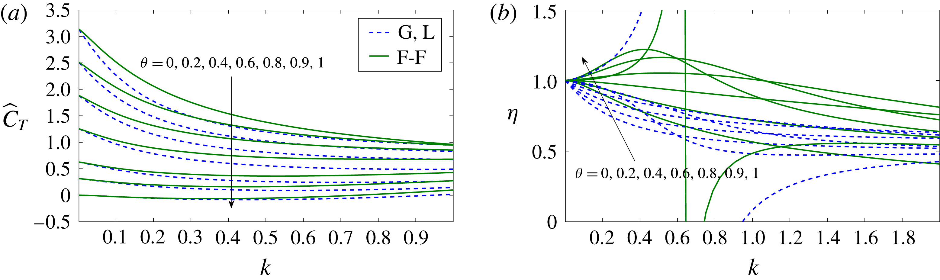
This thrust coefficient and the corresponding propulsive efficiency
 $\unicode[STIX]{x1D702}$
are plotted in figure 2 as functions of the reduced frequency
 $k$
for
 $a=0$
,
 $\unicode[STIX]{x1D719}=90^{\circ }$
and several values of
 $\unicode[STIX]{x1D703}$
, using the functions
 $t_{h}$
,
 $t_{a}$
and
 $t_{ha}$
both from Garrick’s theory and from the impulse theory. The dashed curves, corresponding to Garrick’s thrust, are the same as in figure 9 of Lighthill (Reference Lighthill1969) and in figure 4 for
 $b=0$
of Lighthill (Reference Lighthill1970) (except that
 $2k$
is used there in the abscissa). Both approaches yield the same results for
 $k\rightarrow 0$
, but differ as
 $k$
increases. These differences are especially relevant for the efficiency when
 $k$
is large, as discussed in F-F. Another significant feature of figure 1, and the reason why it is plotted here, is that for
 $\unicode[STIX]{x1D703}$
close to unity the efficiency becomes larger than unity, and even diverges in both formulations for a given
 $k$
of order unity when
 $\unicode[STIX]{x1D703}=1$
(values of the feathering parameter
 $\unicode[STIX]{x1D703}$
larger than unity are not physically relevant, as discussed by Lighthill (Reference Lighthill1969)). This non-physical behaviour of
 $\unicode[STIX]{x1D702}$
, observed in both approaches, is explained by the fact that
 $C_{T}$
remains very small for
 $\unicode[STIX]{x1D703}$
close to unity when
 $k$
is not large (we shall see below that this is not so for large
 $k$
), and the thrust from the potential theory is then a bad approximation because the neglected viscous drag is of the same order or larger.
Plots showing
 $\widehat{C}_{T}$
(a) and
 $\unicode[STIX]{x1D702}$
(b) versus
 $k$
for
 $a=0$
,
 $\unicode[STIX]{x1D719}=90^{\circ }$
and
 $\unicode[STIX]{x1D703}=0,0.2,0.4,0.6,0.8,0.9$
and
 $1$
, computed using Garrick’s expression for the thrust (dashed lines), as in figure 4 in Lighthill (Reference Lighthill1970) (G, L), and from the impulse theory (continuous lines, F-F).

This problem is not restricted to
 $\unicode[STIX]{x1D703}$
near unity because the thrust
 $C_{T}$
defined in (2.1) always goes to zero as
 $k\rightarrow 0$
(note in figure 2 that
 $\widehat{C}_{T}$
goes to a constant as
 $k\rightarrow 0$
, meaning that
 $C_{T}\sim k^{2}$
for small
 $k$
), so that the viscous drag cannot be neglected when
 $k$
is very small. Another consequence of neglecting the (small) viscous drag is that the efficiency always tends to unity as
 $k\rightarrow 0$
(for any finite value of
 $\unicode[STIX]{x1D703}$
). Thus, to circumvent this problem, one may add a constant offset
 $C_{T0}<0$
to
 $C_{T}$
, as done by Mackowski & Williamson (Reference Mackowski and Williamson2015, Reference Mackowski and Williamson2017), representing the quasi-static thrust for
 $k=0$
. Therefore, we define the corrected thrust coefficient
 $$\begin{eqnarray}C_{T}^{c}=C_{T}+C_{T0},\end{eqnarray}$$
with the corresponding
 $\widehat{C}_{T}^{c}$
and
 $\unicode[STIX]{x1D702}^{c}$
computed from their definitions (2.7) and (2.3), respectively. In doing so, the behaviour of the resulting thrust coefficient and propulsive efficiency changes for small and moderate
 $k$
, but remains practically unchanged for sufficiently large
 $k$
.
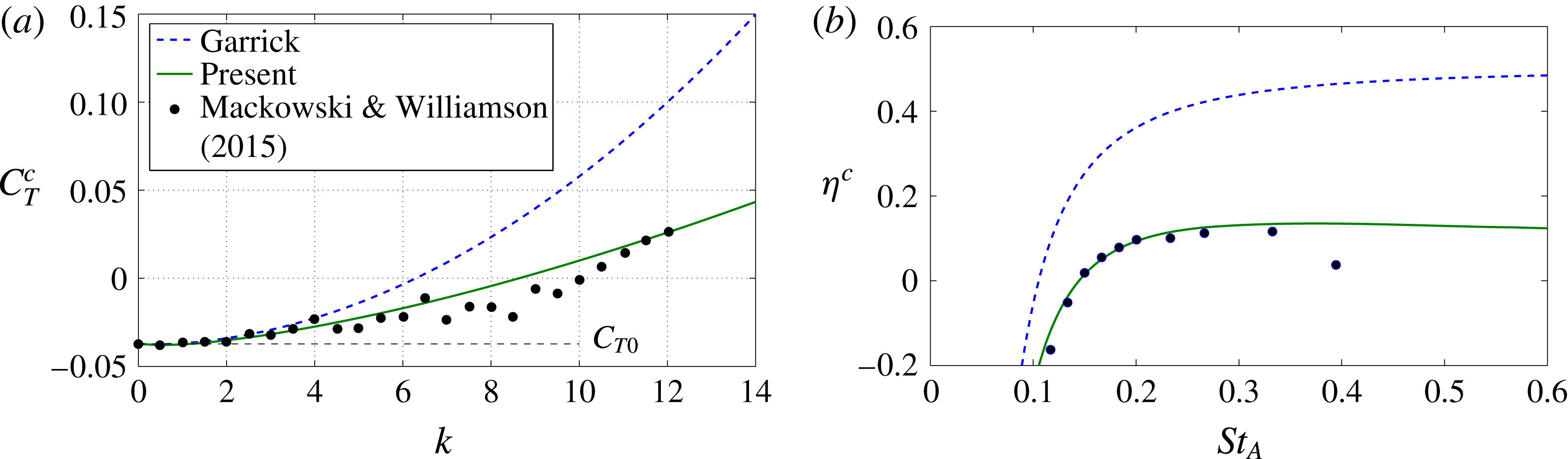
With this correction, the thrust coefficient and the propulsive efficiency from the impulse theory (F-F) fit remarkably well to the experimental data of Mackowski & Williamson (Reference Mackowski and Williamson2015) for a small-amplitude pitching NACA 0012 airfoil, for a wide range of reduced frequencies (figure 3, where their experimental value of the quasi-static thrust
 $C_{T0}=-0.0373$
is used), while the agreement between the experimental data and Garrick’s propulsion with the same constant thrust correction
 $C_{T0}$
is much poorer. With the addition of the quasi-static thrust, the efficiency computed from both approaches improves at low frequencies, but Garrick’s efficiency always goes to a constant (
 $1/2$
) for large frequencies, while the efficiency computed from the vortical impulse theory decays as
 $k^{-1}$
for large
 $k$
, in agreement with experimental results. Note that figure 3(a) coincides with figure 7(a) in F-F, while the efficiency curves plotted in figure 7(b) of F-F were not corrected with
 $C_{T0}$
like those plotted here in figure 3(b).
(a) Comparison of
 $C_{T}^{c}$
versus
 $k$
given by Garrick and by the present theory with the experimental data of Mackowski & Williamson (Reference Mackowski and Williamson2015) for a pitching NACA 0012 airfoil about
 $a=-1/2$
with amplitude
 $\unicode[STIX]{x1D6FC}_{0}=2^{\circ }$
. The dashed horizontal line marks the offset value
 $C_{T0}=-0.0373$
added to both Garrick’s and the present theoretical results. (b) Plot of
 $\unicode[STIX]{x1D702}^{c}$
versus
 $St_{A}=k\times 3\unicode[STIX]{x1D6FC}_{0}/(2\unicode[STIX]{x03C0})$
given by Garrick and by the present theory compared with the same experimental data.

The quasi-static averaged thrust coefficient
 $C_{T0}$
(actually a drag coefficient since it is negative), or asymptote of the averaged thrust coefficient as the frequency
 $k$
approaches zero, has to be obtained experimentally or from full numerical simulations by time-averaging the airfoil’s static drag force through a cycle of oscillation. It does not coincide with the negative of the airfoil’s static profile drag coefficient for any instantaneous position of the airfoil (Mackowski & Williamson Reference Mackowski and Williamson2015, Reference Mackowski and Williamson2017), and depends on the Reynolds number (
 $Re=Uc/\unicode[STIX]{x1D708}$
, with
 $\unicode[STIX]{x1D708}$
the fluid kinematic viscosity), the shape of the airfoil and the kinematics of the flapping motion. The available information in the literature is rather scarce. However, the above-mentioned experimental work by Mackowski & Williamson (Reference Mackowski and Williamson2015, Reference Mackowski and Williamson2017) for pure pitching motion shows that, for sufficiently small
 $\unicode[STIX]{x1D6FC}_{0}$
,
 $C_{T0}$
can roughly be approximated by a constant value, independent of the pivot location
 $a$
and amplitude
 $\unicode[STIX]{x1D6FC}_{0}$
. Since the present formulation is valid only for small flapping amplitudes, this constant value will be selected from these experimental data by Mackowski & Williamson. Instead of using the value
 $C_{T0}=-0.0373$
for
 $\unicode[STIX]{x1D6FC}_{0}=2^{\circ }$
(figure 2), a better average value can be selected from the larger set of experimental data for the thrust coefficient as a function of the non-dimensional pivot location
 $a$
for
 $\unicode[STIX]{x1D6FC}_{0}=8^{\circ }$
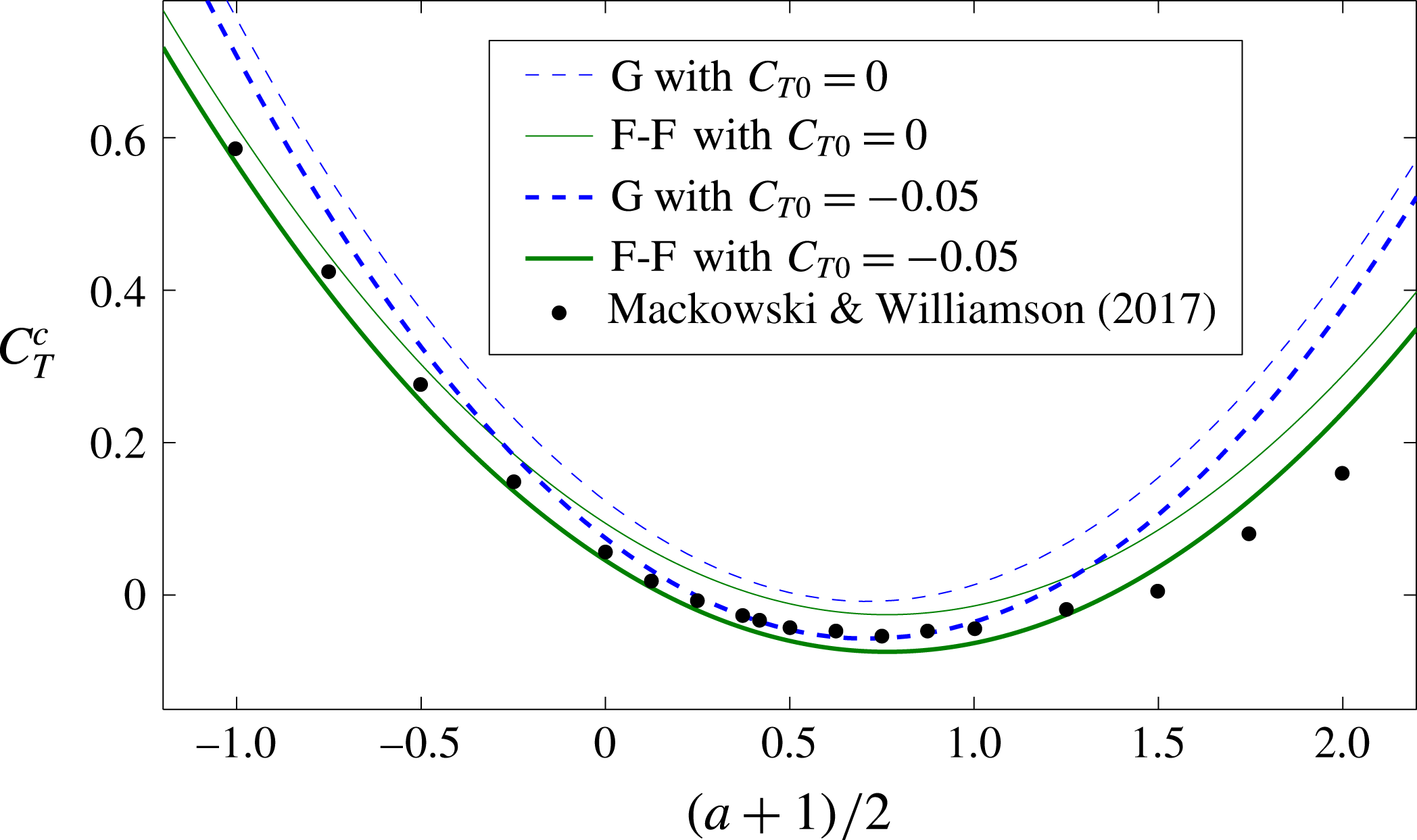
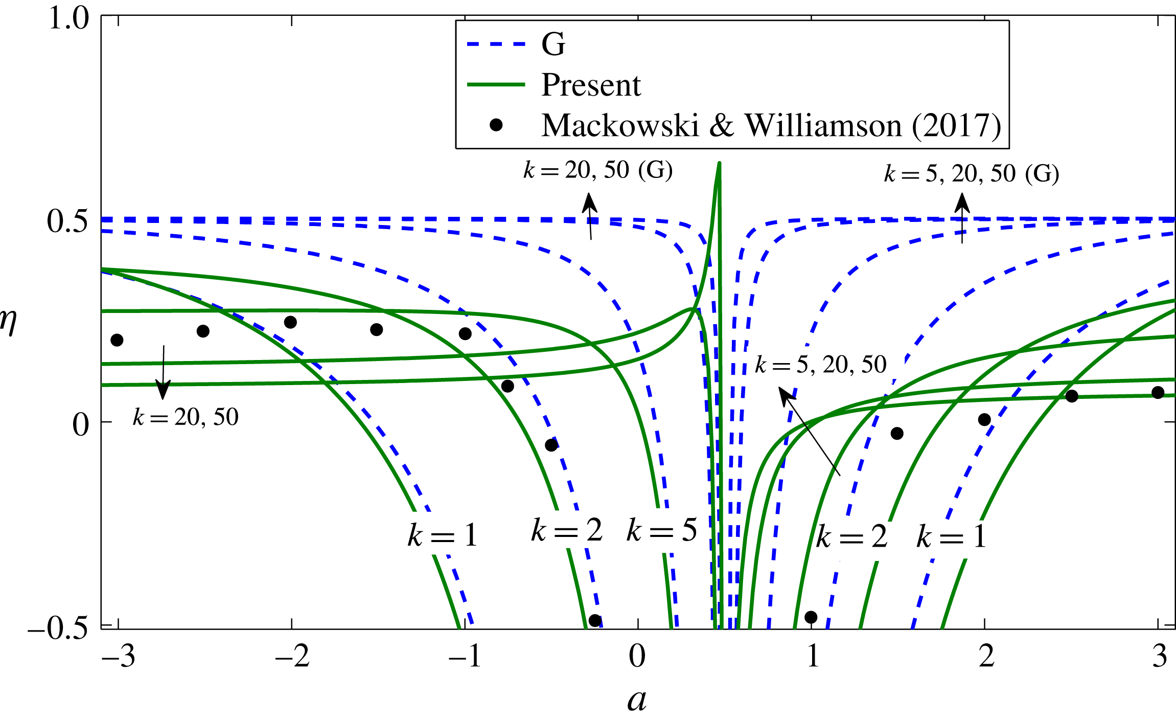
(Mackowski & Williamson Reference Mackowski and Williamson2017). Figure 4 shows that a good fit is achieved with
 $C_{T0}\simeq -0.05$
. Both Garrick’s thrust and the present one corrected with this value of the quasi-static thrust agree reasonably well with the experimental data for pivot locations within the airfoil body (i.e. for
 $-1\leqslant a\leqslant 1$
; note that the non-dimensional pivot location used by these authors is
 $(a+1)/2$
in the present notation). Outside that range, the present theory provides better agreement. These results are for
 $k=2$
, and we know that the disagreement between the two formulations grows with
 $k$
(e.g. figure 3).
Comparison of
 $C_{T}$
versus the non-dimensional pivot location given by Garrick (G) and by the present (F-F) theory with the experimental data of Mackowski & Williamson (Reference Mackowski and Williamson2017) for a pitching NACA 0012 airfoil with
 $k=2$
and
 $\unicode[STIX]{x1D6FC}_{0}=8^{\circ }$
at
 $Re=16\,000$
, both without adding a quasi-static thrust (
 $C_{T0}=0$
) and for
 $C_{T0}=-0.05$
.

Accordingly, this value
 $C_{T0}=-0.05$
will be selected in all the computations reported below. We shall see that the results for the optimal efficiency remain almost unaltered when a slightly different constant value of
 $C_{T0}$
is selected (see e.g. figures 5 and 8 below, where results computed with
 $C_{T0}=0$
and
 $-0.025$
are also plotted and discussed in relation to those obtained with
 $C_{T0}=-0.05$
).
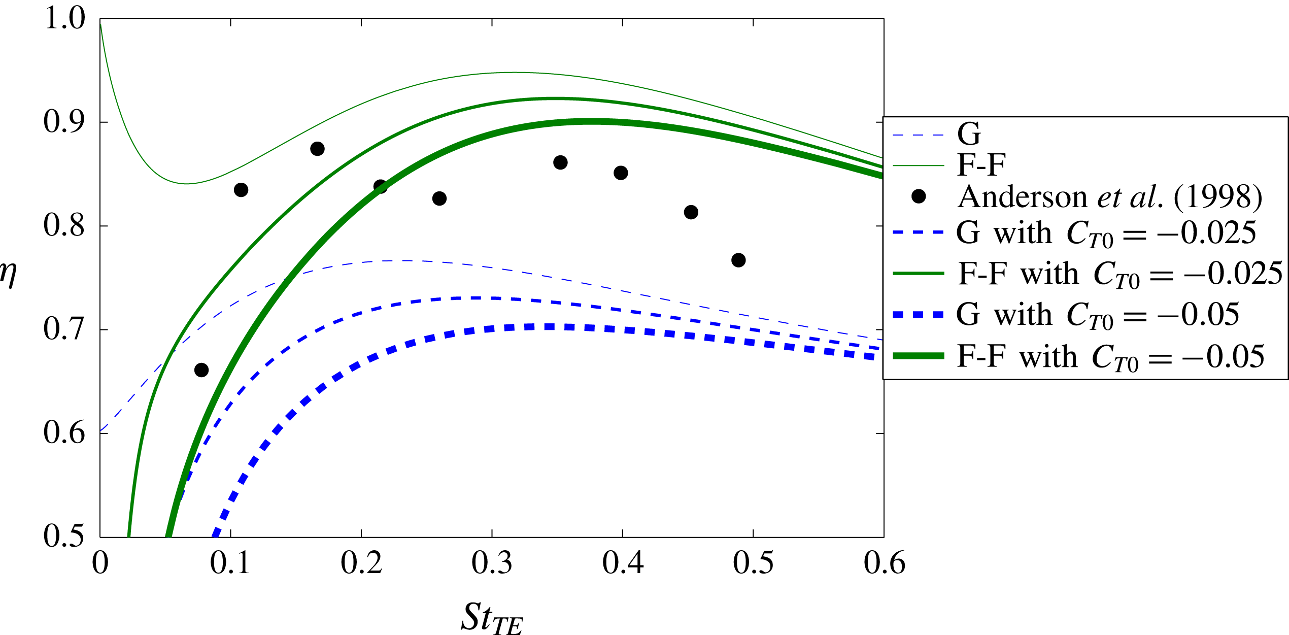
Comparison with the experimental results for the efficiency versus the Strouhal number based on the peak-to-peak trailing-edge excursion
 $St_{TE}$
corresponding to case 1 in figure 5 of Anderson et al. (Reference Anderson, Streitlien, Barret and Triantafyllou1998) (
 $a=-1/3$
,
 $h_{0}=1.5$
,
 $\unicode[STIX]{x1D719}=75^{\circ }$
, and varying
 $\unicode[STIX]{x1D6FC}_{0}$
such that the maximum angle of attack is
 $21^{\circ }$
). Dashed lines are for Garrick’s thrust (G) and continuous lines for the thrust from the impulse theory (F-F). Curves with three values of the offset
 $C_{T0}$
,
 $0,-0.025$
and
 $-0.05$
, are plotted.

It is remarkable that the present propulsive efficiency from linear potential theory, with the correct decay for large frequencies resulting from the vortical impulse theory and modified at small frequencies with
 $C_{T0}$
, agrees reasonably well with experimental data not only for small amplitudes of the oscillation as in figures 3 and 4, but also for large amplitudes where the linearity hypothesis is no longer valid. For instance, figure 5 shows a comparison with the experimental results of Anderson et al. (Reference Anderson, Streitlien, Barret and Triantafyllou1998) for the efficiency of a heaving and pitching NACA 0012 airfoil at Reynolds number
 $40\,000$
, pitching about
 $a=-1/3$
(one-third chord pivot point), with high heave and pitching amplitudes (
 $h_{0}=1.5$
and varying
 $\unicode[STIX]{x1D6FC}_{0}$
such that the maximum angle of attack in each cycle is
 $21^{\circ }$
), and with a phase shift
 $\unicode[STIX]{x1D719}=75^{\circ }$
. This case corresponds, approximately, to the highest efficiency found experimentally by these authors,
 $\unicode[STIX]{x1D702}\simeq 0.87$
, which is reached for a Strouhal number based on the peak-to-peak trailing-edge excursion
 $St_{TE}\simeq 0.36$
(the first peak of
 $\unicode[STIX]{x1D702}$
at
 $St_{TE}$
approximately
 $0.15$
‘is not significant for applications because the thrust coefficient is typically very small’, as noted by these authors). It is observed in figure 5 that this peak is reasonably well captured by the potential theory from the impulse theory when corrected with a constant
 $C_{T0}$
, especially in relation to the optimum value of
 $St_{TE}$
(or frequency). In any case, the efficiency computed from Garrick’s thrust corrected with the same value of
 $C_{T0}$
shows much poorer agreement with the experimental data, predicting a significantly lower
 $St_{TE}$
. Since no data for the quasi-static thrust coefficient are given in Anderson et al. (Reference Anderson, Streitlien, Barret and Triantafyllou1998), figure 5 shows the curves for two different values of
 $C_{T0}$
, with better agreement when using
 $C_{T0}=-0.05$
, but with no significant difference in relation to the optimal frequency for the highest efficiency when using half this value.
In summary, the thrust computed from the impulse theory for linear potential flows and corrected with an appropriate constant offset
 $C_{T0}$
, representing the quasi-static thrust, provides a good approximation for estimating the conditions that optimize propulsive efficiency of heaving and pitching airfoils. To simplify the notation, the superscript ‘
 $c$
’ in
 $C_{T}^{c}$
,
 $\widehat{C}_{T}^{c}$
and
 $\unicode[STIX]{x1D702}^{c}$
will be dropped in what follows.
3 Maximizing the propulsive efficiency
3.1 Pure pitching motion
Let us start with the simplest case of a pure pitching motion (
 $h_{0}=0$
). In this case,
 $$\begin{eqnarray}C_{T}=t_{a}(k,a)\unicode[STIX]{x1D6FC}_{0}^{2}+C_{T0},\quad \unicode[STIX]{x1D702}=\frac{t_{a}(k,a)+C_{T0}/\unicode[STIX]{x1D6FC}_{0}^{2}}{p_{a}(k,a)},\end{eqnarray}$$
so that
 $\unicode[STIX]{x1D702}$
depends not only on
 $k$
and
 $a$
, but also on
 $\unicode[STIX]{x1D6FC}_{0}$
owing to the addition of the quasi-static thrust constant
 $C_{T0}$
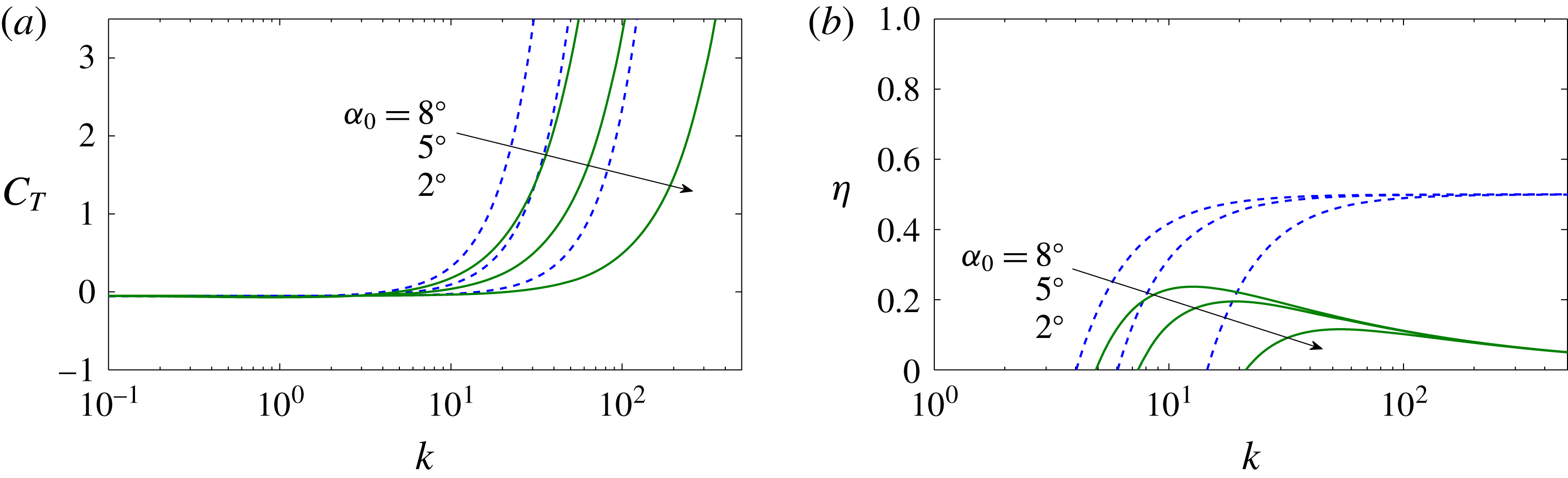
. Figure 6 shows the effect of
 $\unicode[STIX]{x1D6FC}_{0}$
on the variation with
 $k$
of
 $C_{T}$
and
 $\unicode[STIX]{x1D702}$
for a given pitching axis
 $a$
. When computed with Garrick’s theory, the maximum efficiency is
 $1/2$
in all cases, always reached for
 $k\rightarrow \infty$
. From the present theory, however, the maximum efficiency is reached at a finite value
 $k_{m}$
that increases with decreasing
 $\unicode[STIX]{x1D6FC}_{0}$
for given
 $a$
. The maximum efficiency
 $\unicode[STIX]{x1D702}_{max}(k_{m})$
obviously increases with
 $\unicode[STIX]{x1D6FC}_{0}$
for a given
 $C_{T0}<0$
. But we are mostly interested in the behaviour of
 $\unicode[STIX]{x1D702}_{max}$
and
 $k_{m}$
as the pitching location
 $a$
is varied, so that a representative small value of
 $\unicode[STIX]{x1D6FC}_{0}$
(
 $8^{\circ }$
, say) is selected.
Plots of
 $C_{T}$
(a) and
 $\unicode[STIX]{x1D702}$
(b) versus
 $k$
for a pure pitching motion (
 $h_{0}=0$
) with
 $a=0$
, computed with
 $C_{T0}=-0.05$
and three different values of
 $\unicode[STIX]{x1D6FC}_{0}$
according to Garrick (dashed lines) and according to F-F (continuous lines).

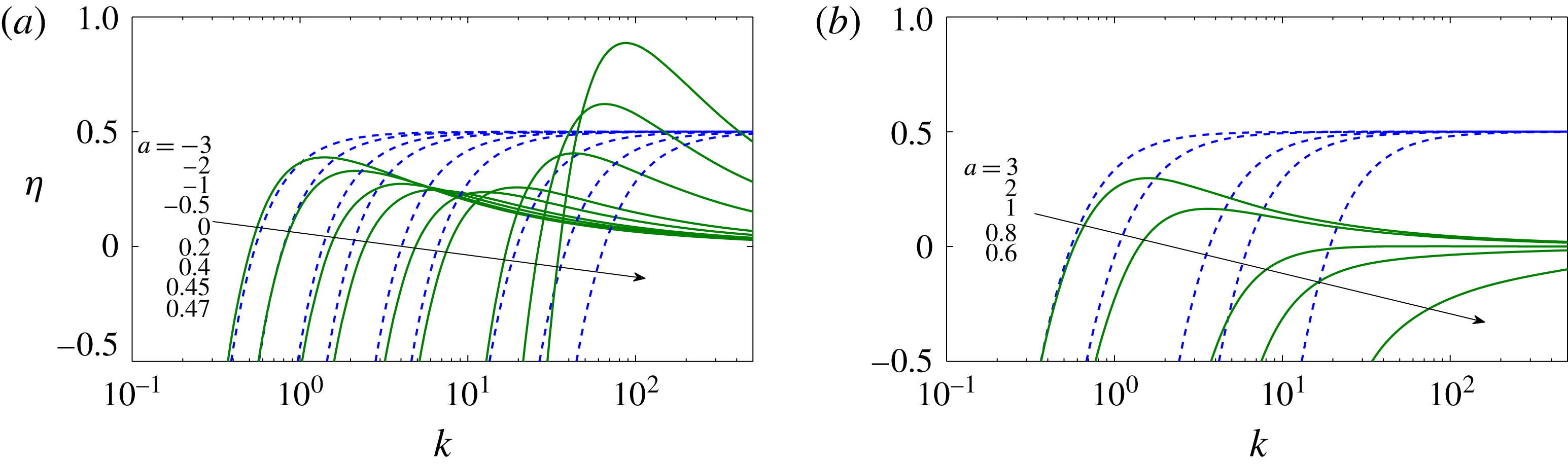
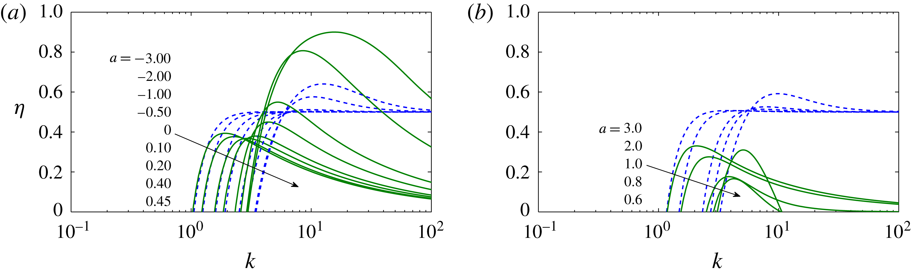
Figure 7 compares
 $\unicode[STIX]{x1D702}(k)$
for several values of
 $a$
, computed with
 $C_{T0}=-0.05$
from Garrick’s thrust and from the present formulation. Pivot locations outside the airfoil chord length
 $-1\leqslant a\leqslant 1$
are also considered. The maximum propulsive efficiency from Garrick’s thrust is always
 $1/2$
, reached for
 $k\rightarrow \infty$
independently of the value of
 $a$
, while in the present formulation it is obtained at a finite value of
 $k$
that depends on
 $a$
, as in the experimental data. But this being a relevant difference, the most substantial ones are (1) that according to the present theory the maximum efficiency is obtained for
 $a=1/2$
, i.e. for the airfoil pitching about three-quarters of its chord length, and (2) that for
 $1/2<a<1$
there is no thrust production but just drag (
 $C_{T}<0$
) for all values of
 $k$
, tending to zero as
 $k$
goes to infinity (figure 7
b). For pivot locations outside the airfoil, the maximum efficiency is again positive and increases with the distance of the pitching axis from the airfoil body, both downstream (
 $a>1$
) and upstream (
 $a<-1$
), more rapidly in the latter case (figure 7
a).
Plot of
 $\unicode[STIX]{x1D702}$
versus
 $k$
for a pure pitching motion (
 $h_{0}=0$
with
 $\unicode[STIX]{x1D6FC}_{0}=8^{\circ }$
) for several values of
 $a$
, as indicated, computed according to Garrick (dashed lines) and according to F-F (continuous lines), both with
 $C_{T0}=-0.05$
.

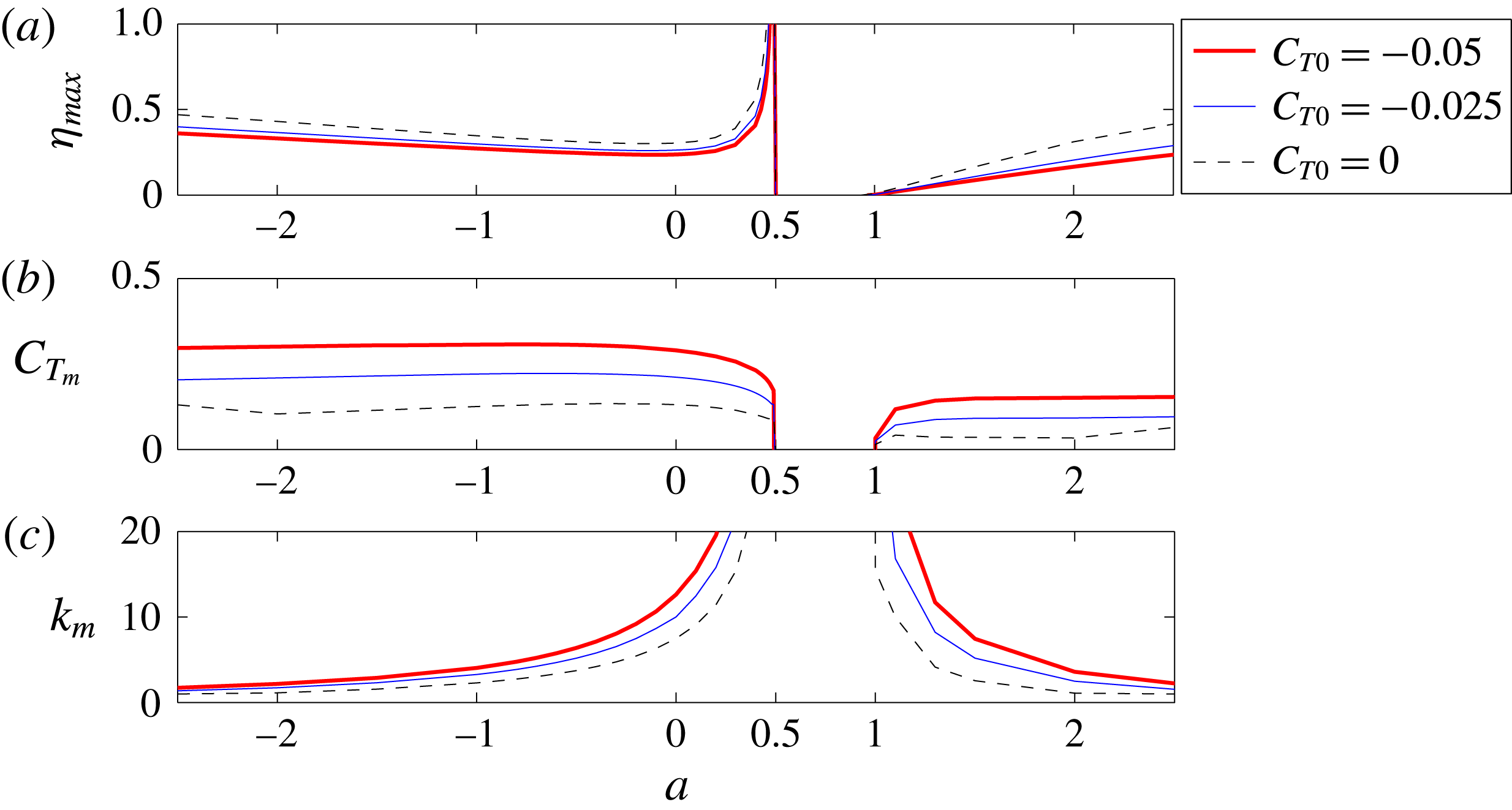
Plots of
 $\unicode[STIX]{x1D702}_{max}$
versus
 $a$
(a) and the corresponding
 $C_{T_{m}}$
and
 $k_{m}$
(b,c) for a pure pitching motion (
 $h_{0}=0$
), computed with
 $C_{T0}=0,~-0.025$
and
 $-0.05$
, and with
 $\unicode[STIX]{x1D6FC}_{0}=8^{\circ }$
. The airfoil’s body is in
 $-1\leqslant a\leqslant 1$
.

Figure 8 summarizes
 $\unicode[STIX]{x1D702}_{max}$
versus the pitching axis
 $a$
, and the corresponding values
 $k_{m}(a)$
and
 $C_{T_{m}}(a)$
. For reference, the results obtained with
 $C_{T0}=0$
and
 $C_{T0}=-0.025$
are also included in figure 8. It must be noted that as
 $a\rightarrow 1/2$
from the left,
 $\unicode[STIX]{x1D702}_{max}\rightarrow \infty$
, which is not physical, but corresponds to unphysical
 $k\rightarrow \infty$
with
 $C_{T_{m}}\rightarrow 0$
. Both
 $C_{T_{m}}$
and
 $\unicode[STIX]{x1D702}_{m}$
remain negative for pivot locations between the three-quarter chord and the trailing edge (
 $1/2<a<1$
). Beyond the trailing edge (
 $a>1$
), the maximum efficiency becomes positive again, increasing with
 $a$
, with
 $k_{m}$
decreasing from infinity. Finally, for pivot locations ahead of the leading edge (
 $a<-1$
),
 $\unicode[STIX]{x1D702}_{m}$
continues increasing monotonically, with decreasing
 $k_{m}$
and very slowly decreasing
 $C_{T_{m}}$
.
Thus, the present linearized potential theory indicates that the maximum propulsive efficiency is obtained for
 $a$
close to, but less than,
 $1/2$
, for a relatively high reduced frequency and corresponding to a relatively low thrust force. With
 $C_{T0}=-0.05$
, the maximum efficiency is above
 $1/2$
for
 $0.43\lesssim a<1/2$
. For this
 $C_{T0}$
,
 $\unicode[STIX]{x1D702}_{max}$
reaches a minimum of approximately
 $0.24$
for a pivot point close to the centre of the airfoil (for
 $a\simeq -0.1$
), and remains almost constant for pivot locations within the airfoil body, but associated with relatively high thrust, which reaches a maximum for
 $a\simeq -3/4$
. It is observed that the resulting
 $\unicode[STIX]{x1D702}_{m}$
and
 $k_{m}$
for given
 $a$
do not depend too much on the selected value of
 $C_{T0}$
. However,
 $C_{T_{m}}$
is obviously very sensitive to the selected quasi-static thrust offset, but its qualitative behaviour with varying
 $a$
remains almost unchanged when
 $|C_{T0}|$
increases from zero.
To further analyse these results and the differences between Garrick’s and the present efficiency, figure 9 shows the variation of the efficiency
 $\unicode[STIX]{x1D702}$
with the pitching axis location
 $a$
for several values of
 $k\geqslant 1$
(for
 $0<k<1$
,
 $\unicode[STIX]{x1D702}<0$
for almost all the values of
 $a$
considered in the figure). For each
 $k$
, there exists an interval of values of
 $a$
that always includes part (or all) of the extension of the airfoil’s body
 $-1\leqslant a\leqslant 1$
, where
 $\unicode[STIX]{x1D702}$
is negative. The length of this interval where only drag forces are produced decreases with increasing
 $k$
. For
 $k\rightarrow \infty$
, it is reduced to just the neighbourhood of
 $a=1/2$
when one uses Garrick’s propulsion expression, or to the interval
 $[1/2,1]$
when using the present formulation. The maximum propulsion efficiency according to Garrick’s theory is
 $1/2$
for all
 $k$
, reached for pivot location further from the airfoil’s body (ahead of the leading edge, or behind the trailing edge) when
 $k$
is small. With the present theory, the maximum of
 $\unicode[STIX]{x1D702}$
is also reached for a pivot point further from the airfoil’s body when
 $k$
is small (remember that the differences with Garrick’s theory become smaller as
 $k$
decreases), but above a certain value of
 $k$
the maximum is reached for a finite
 $a$
, which tends to
 $a=1/2^{-}$
as
 $k\rightarrow \infty$
, as discussed above. For the cases plotted in figure 9, this happens for
 $k\geqslant 5$
. For sufficiently large
 $k$
, one finds the pronounced peak of
 $\unicode[STIX]{x1D702}$
near
 $a=1/2^{-}$
commented on above, which is larger than one-half for
 $k\gtrsim 40$
in the present case with
 $C_{T0}=-0.05$
and
 $\unicode[STIX]{x1D6FC}_{0}=8^{\circ }$
.
Plot of
 $\unicode[STIX]{x1D702}$
versus
 $a$
for a pure pitching motion (
 $h_{0}=0$
, with
 $\unicode[STIX]{x1D6FC}_{0}=8^{\circ }$
) for several values of
 $k$
, as indicated, computed according to Garrick (dashed lines, G) and according to F-F (continuous lines), both with
 $C_{T0}=-0.05$
. The dots are experimental data from Mackowski & Williamson (Reference Mackowski and Williamson2017) for
 $k=2$
. Remember that the pivot point is within the foil for
 $-1<a<1$
.

These results are in reasonable agreement with experimental data for
 $k=2$
obtained by Mackowski & Williamson (Reference Mackowski and Williamson2017), also shown in figure 9. The maximum propulsive efficiency in this case is reached at
 $a\simeq -2$
(pitching axis approximately a half-chord length ahead of the leading edge), while in the linear theory the efficiency peaks at that pivot location when
 $k$
is slightly larger (for
 $k=5$
, shown in the figure,
 $\unicode[STIX]{x1D702}$
peaks at
 $a\simeq -1$
, the leading edge). But the agreement between the experimental data and the present linear theory for
 $k=2$
is remarkable when
 $a>-1$
.
It should be noted that the unphysical efficiency (larger than unity) when
 $a\rightarrow 0.5^{-}$
for large
 $k$
is due to the fact that the power coefficient
 $C_{P}$
reaches a sharp minimum for
 $a=0.5$
, already discussed by Lighthill (Reference Lighthill1970), which is particularly small for a pure pitching motion. In (2.3)
 $C_{P}$
is the same in both approaches. The difference is that
 $C_{T}$
in Garrick’s theory also has a sharp minimum at
 $a=0.5$
, while in the present theory the sharp minimum of
 $C_{T}$
is slightly displaced to
 $a=0.5^{+}$
(when
 $k$
is large). But both theories predict unphysical
 $\unicode[STIX]{x1D702}>1$
for
 $a=0.5$
when
 $C_{T0}\neq 0$
. However, the present theory yields the correct asymmetry of
 $\unicode[STIX]{x1D702}$
in relation to
 $a=0.5$
for a given
 $k$
observed in the experiments, which is not predicted by Garrick’s theory (figure 9). This asymmetry is due to the displacement of the sharp minimum of
 $C_{T}$
towards
 $a>0.5$
for sufficiently large
 $k$
(see also figure 13).
3.2 General heaving and pitching motion
For a combined heaving and pitching motion with constant values of
 $\unicode[STIX]{x1D719}$
and
 $\unicode[STIX]{x1D703}$
, the qualitative behaviour of
 $\unicode[STIX]{x1D702}$
versus
 $k$
as the pivot location
 $a$
is varied is similar to that described above for a pure pitching motion (which corresponds to
 $\unicode[STIX]{x1D703}\rightarrow \infty$
). For a given constant
 $C_{T0}$
, the results also depend slightly on the heaving amplitude
 $h_{0}$
, in a similar way to the dependence on
 $\unicode[STIX]{x1D6FC}_{0}$
of
 $\unicode[STIX]{x1D702}$
for a pure pitching motion discussed above:
 $$\begin{eqnarray}\unicode[STIX]{x1D702}=\frac{t_{h}+t_{a}\unicode[STIX]{x1D703}^{2}+t_{ha}\unicode[STIX]{x1D703}+C_{T0}/(kh_{0})^{2}}{p_{h}+p_{a}\unicode[STIX]{x1D703}^{2}+p_{ha}\unicode[STIX]{x1D703}}.\end{eqnarray}$$
All the results reported below are computed with
 $C_{T0}=-0.05$
and the relatively small value
 $h_{0}=0.1$
.
Plots of
 $\unicode[STIX]{x1D702}$
versus
 $k$
for heaving and pitching motion with
 $\unicode[STIX]{x1D703}=0.6$
and
 $\unicode[STIX]{x1D719}=90^{\circ }$
for several values of
 $a$
, as indicated, computed according to Garrick (dashed lines) and according to F-F (continuous lines), both with
 $C_{T0}=-0.05$
and
 $h_{0}=0.1$
.

The particular case of a pure heaving motion is not considered separately because it corresponds to
 $\unicode[STIX]{x1D703}=0$
. It should be noted that this pure vertical motion is equivalent to a combined motion in the limit of a pitching axis location very far away from the airfoil,
 $|a|\rightarrow \infty$
. This equivalence is easily checked by taking that limit in
 $\unicode[STIX]{x1D702}$
with the help of the analytical expressions given in appendix A.
Figure 10 shows the evolution of the efficiency
 $\unicode[STIX]{x1D702}$
with
 $k$
for several values of the pitching axis location
 $a$
when
 $\unicode[STIX]{x1D703}=0.6$
and the phase shift is
 $\unicode[STIX]{x1D719}=90^{\circ }$
. The results are quite similar to those in figure 7: the maximum efficiency is reached as
 $a\rightarrow 1/2$
, with corresponding frequency
 $k_{m}$
tending to infinity and corresponding thrust
 $\widehat{C}_{T_{m}}$
going to zero, so that the physical conditions for optimal propulsion according to the present theory, for a given feathering parameter
 $\unicode[STIX]{x1D703}$
and phase shift
 $\unicode[STIX]{x1D719}$
, correspond to a pitching axis
 $a$
close to, but less than,
 $1/2$
. As the pivot location moves away from the airfoil’s body, ahead of the leading edge or behind the trailing edge,
 $\unicode[STIX]{x1D702}_{m}$
also increases, but the main difference from the pure pitching case is that the corresponding values of
 $k_{m}$
are significantly smaller.
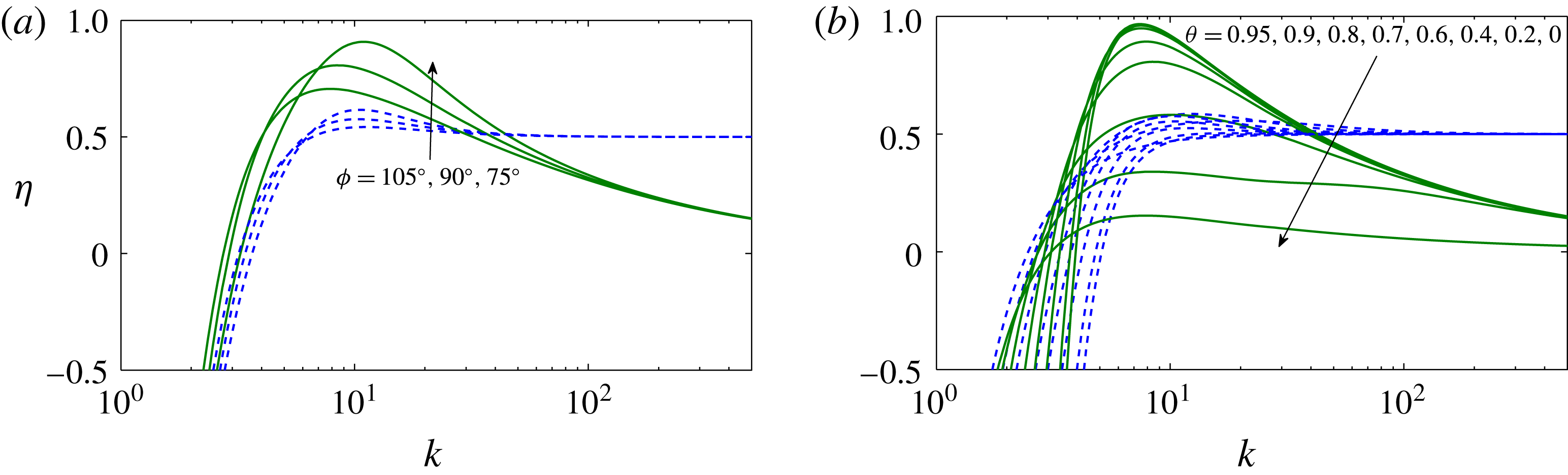
Plots of
 $\unicode[STIX]{x1D702}$
versus
 $k$
for a heaving and pitching motion about
 $a=0.4$
for several values of
 $\unicode[STIX]{x1D719}$
with
 $\unicode[STIX]{x1D703}=0.6$
(a), and for several values of
 $\unicode[STIX]{x1D703}$
with
 $\unicode[STIX]{x1D719}=90^{\circ }$
(b), computed according to Garrick (dashed lines) and according to F-F (continuous lines), both with
 $C_{T0}=-0.05$
and
 $h_{0}=0.1$
.

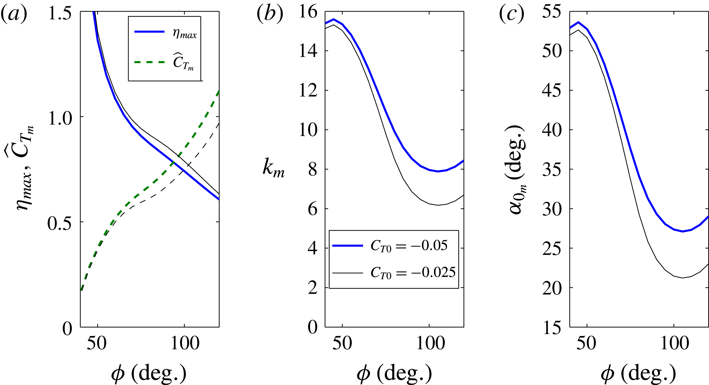
Plots of
 $\unicode[STIX]{x1D702}_{max}$
and
 $\widehat{C}_{T_{m}}$
versus
 $\unicode[STIX]{x1D719}$
(a) and the corresponding
 $k_{m}$
and
 $\unicode[STIX]{x1D6FC}_{0m}$
(b,c) for
 $a=0.4$
and
 $\unicode[STIX]{x1D703}=0.6$
, with
 $h_{0}=0.1$
. Thick lines are computed with
 $C_{T0}=-0.05$
, and thin lines with
 $C_{T0}=-0.025$
.

For other values of
 $\unicode[STIX]{x1D719}$
or
 $\unicode[STIX]{x1D703}$
the overall behaviour is quite similar to that depicted in figure 10, the differences being quantitative rather than qualitative. Figure 11 compares the results for several values of
 $\unicode[STIX]{x1D719}$
and
 $\unicode[STIX]{x1D703}$
at the high-frequency peak of the efficiency as
 $a$
approaches
 $(1/2)^{-}$
, in particular for
 $a=0.4$
. It is observed (figure 11
a) that the efficiency peak increases when
 $\unicode[STIX]{x1D719}$
decreases for a given
 $\unicode[STIX]{x1D703}$
, reaching non-physical values larger than unity (see figure 12
a). But this is because the corresponding values of
 $\unicode[STIX]{x1D6FC}_{0m}$
become so large as
 $\unicode[STIX]{x1D719}$
decreases that the present linear theory cannot be valid for the selected values of
 $\unicode[STIX]{x1D703}$
and
 $h_{0}$
. Figure 12(c) shows that this is so in the present case when
 $\unicode[STIX]{x1D719}$
becomes sufficiently smaller than
 $90^{\circ }$
(
 $\unicode[STIX]{x1D719}\lesssim 75^{\circ }$
). In addition, as
 $\unicode[STIX]{x1D719}$
decreases, the corresponding thrust
 $\widehat{C}_{T_{m}}$
decreases very rapidly and the corresponding
 $k_{m}$
increases. Therefore, the optimum propulsion efficiency for a given
 $\unicode[STIX]{x1D703}$
according to the present linear theory is reached for a pivot point
 $a$
close to, but less than,
 $1/2$
(three-quarter chord pitching), with a phase shift
 $\unicode[STIX]{x1D719}$
smaller than
 $90^{\circ }$
, between approximately
 $75^{\circ }$
and
 $90^{\circ }$
. These results are not significantly modified when a different constant value of
 $C_{T0}$
is selected, as shown in figure 12 when
 $C_{T0}$
is halved.
(a) Plot of
 $\unicode[STIX]{x1D702}$
versus
 $a$
for
 $\unicode[STIX]{x1D703}=0.9$
,
 $\unicode[STIX]{x1D719}=75^{\circ }$
and several values of
 $k$
, as indicated, computed according to Garrick (dashed lines) and according to F-F (continuous lines), both with
 $C_{T0}=-0.05$
and
 $h_{0}=0.1$
. (b) Detail for
 $k=4$
and
 $k=5.5$
near
 $a=1/2$
, showing also the corresponding curves for
 $\widehat{C}_{T}$
(red dashed lines).

In relation to the optimum value of the feathering parameter
 $\unicode[STIX]{x1D703}$
, figure 11(b) shows that, for
 $\unicode[STIX]{x1D719}=90^{\circ }$
and
 $a=0.4$
, the peak of the propulsive efficiency increases with
 $\unicode[STIX]{x1D703}$
until
 $\unicode[STIX]{x1D703}\simeq 0.9$
, and then decreases. As a difference with decreasing
 $\unicode[STIX]{x1D719}$
, the corresponding
 $k_{m}$
,
 $\widehat{C}_{T_{m}}$
and
 $\unicode[STIX]{x1D6FC}_{0m}$
remain almost unchanged. Therefore, the optimum value of
 $\unicode[STIX]{x1D703}$
predicted by the present linear theory for the high-frequency peak of the efficiency about three-quarter chord pitching is approximately
 $0.9$
.
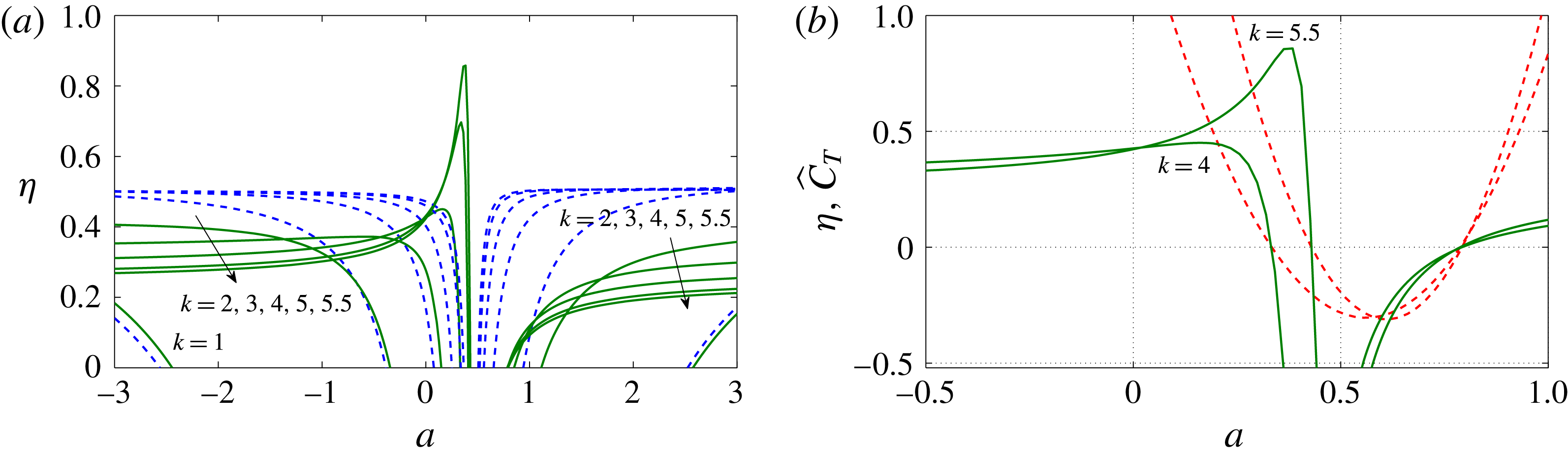
Finally, to better illustrate these conditions that maximize the propulsion efficiency, figure 13 shows
 $\unicode[STIX]{x1D702}$
as a function of the pitching axis
 $a$
for several values of the reduced frequency when
 $\unicode[STIX]{x1D703}=0.9$
and
 $\unicode[STIX]{x1D719}=75^{\circ }$
. A pronounced peak of the efficiency is observed for reduced frequencies larger than approximately
 $5$
when
 $a$
is close to, but less than,
 $1/2$
. For slightly larger values of
 $a$
, the efficiency drops abruptly, and for
 $1/2<a\lesssim 1$
it becomes negative. This behaviour is not observed when Garrick’s thrust is used to compute the efficiency (also shown). Figure 13(b) shows that the thrust coefficient corresponding to this efficiency peak for
 $k=5.5$
is relatively small (but, of course, positive) when compared with the thrust coefficient corresponding to a lower-efficiency peak for a smaller value of
 $k$
(
 $k=4$
, say).
4 Conclusion
It is shown in this paper that the conditions that maximize the propulsive efficiency of a harmonically heaving and pitching airfoil predicted by the thrust coefficient from the linear potential theory when properly computed from a general vortical impulse formulation, and corrected at low frequencies by adding a constant quasi-static thrust, are quite different from those predicted by Garrick’s thrust with the same quasi-static thrust correction. It is found that the maximum peak of propulsive efficiency is reached for sufficiently high reduced frequencies when the pitching axis is located close to, but ahead of, the three-quarter chord point. This is valid both for a pure pitching motion and for a combined pitching and heaving motion of the airfoil. In the last general case, optimal conditions are found for a feathering parameter of approximately
 $0.9$
and a pitching–heaving phase shift between approximately
 $75^{\circ }$
and
 $90^{\circ }$
. These conditions always correspond to relatively low values of the thrust coefficient, but it increases rapidly as the reduced frequency decreases, at the cost of slightly reducing the efficiency peak. Further, the theory predicts that no propulsion force is generated (i.e. flapping generates just drag) when the pitching axis is located behind the three-quarter chord point, recovering positive thrust when the pivot point is at, or very close to, the trailing edge of the airfoil, depending on the flapping parameters. For a pitching axis sufficiently behind the trailing edge, and ahead of the leading edge, lower-efficiency peaks are also found corresponding to smaller values of the reduced frequency.
These results are qualitative, rather than quantitative, because the linear approximation restricts the results to small amplitudes of the pitching and heaving motions of the airfoil. Moreover, the constant value of the added quasi-static thrust coefficient, which is justified from available experimental data for small flapping amplitudes, introduces the additional dependence of the propulsion efficiency on the flapping amplitude,
 $\unicode[STIX]{x1D6FC}_{0}$
in the case of pure pitching motion or
 $h_{0}$
in the combined flapping motion (which are related through the feathering parameter
 $\unicode[STIX]{x1D703}$
in the combined motion). Thus, in this last general case, even selecting very small values of
 $h_{0}$
, the resulting optimal conditions for propulsive efficiency may correspond to large values of
 $\unicode[STIX]{x1D6FC}_{0}$
for which the approximation is no longer valid. For this reason, the theory predicts general trends of the non-dimensional parameters that generate an increase of the propulsive efficiency, sometimes without bound because the validity limits of the linear theory are largely trespassed. Additionally, the exact value of the efficiency depends on the particular (constant) quasi-static thrust selected to correct the potential thrust coefficient at small frequencies.
The thrust coefficient and propulsive efficiency of the present formulation are checked here (and in F-F) against some available experimental data, with remarkable agreement, even when the amplitude is not so small. These experimental data for small amplitudes, mostly for pure pitching motions of the airfoil, are for pitching axis locations and reduced frequencies outside the optimal ranges predicted here. Since the specific conditions that maximize the propulsion efficiency found here are so different from those predicted from Garrick’s classical thrust, it would be of interest to check them experimentally.
It is believed that the analytical formulation given here, which corrects the formulation developed in F-F with a quasi-static constant drag at low frequencies, may be a useful tool for examining conditions associated with optimal propulsion performance, just as the classical linear potential theory for the lift continues to be used today. The present results may lead to new advances in unsteady aerodynamics. In particular, the predictions for optimal propulsion found in this paper, and especially those related to the pitching axis, may have implications for the design of bio-inspired propulsors in flapping-wing vehicles, both aerial and aquatic.
Acknowledgements
This research was supported by the Ministerio de Economía y Competitividad of Spain grants no. DPI2013-40479-P and DPI2016-76151-C2-1-R.
Appendix A. Functions
 $t_{h}$
,
$t_{a}$
,
$t_{ha}$
,
$p_{h}$
,
$p_{a}$
and
$p_{ha}$


For easy reference, the functions
 $t_{h}(k)$
,
 $t_{a}(k,a)$
and
 $t_{ha}(k,a,\unicode[STIX]{x1D719})$
appearing in the time-averaged thrust coefficient
 $C_{T}$
(2.1) are reproduced here. From Garrick’s (Reference Garrick1936) propulsion theory, these functions can be written as
 $$\begin{eqnarray}t_{h}(k)=\unicode[STIX]{x03C0}[F^{2}(k)+G^{2}(k)],\end{eqnarray}$$
 $$\begin{eqnarray}\displaystyle t_{a}(k,a) & = & \displaystyle \unicode[STIX]{x03C0}[(1+(a-{\textstyle \frac{1}{2}})^{2}k^{2})|C(k)|^{2}+(a-{\textstyle \frac{1}{2}})(F(k)-{\textstyle \frac{1}{2}})k^{2}\nonumber\\ \displaystyle & & \displaystyle -\,(a+{\textstyle \frac{1}{2}})kG(k)-F(k)\!],\end{eqnarray}$$
 $$\begin{eqnarray}\displaystyle t_{ha}(k,a,\unicode[STIX]{x1D719}) & = & \displaystyle \unicode[STIX]{x03C0}\left[(-2|C(k)|^{2}+kG(k)+F(k))\sin \unicode[STIX]{x1D719}\right.\nonumber\\ \displaystyle & & \displaystyle \left.+\left(k(2a-1)|C(k)|^{2}+kF(k)-G(k)-\frac{k}{2}\right)\cos \unicode[STIX]{x1D719}\right],\end{eqnarray}$$
where
 $C(k)=F(k)+\text{i}G(k)$
is the complex Theodorsen’s function (Theodorsen Reference Theodorsen1935; Garrick Reference Garrick1938). According to the general vortical impulse theory, these functions can be written as (Fernandez-Feria Reference Fernandez-Feria2016)
 $$\begin{eqnarray}\displaystyle & \displaystyle t_{h}(k)=-2G_{1}(k), & \displaystyle\end{eqnarray}$$
 $$\begin{eqnarray}\displaystyle & \displaystyle t_{a}(k,a)=-[2\unicode[STIX]{x03C0}F(k)+2akF_{1}(k)+2(2+k^{2}(a-1)(a-{\textstyle \frac{1}{2}}))G_{1}(k)], & \displaystyle\end{eqnarray}$$
 $$\begin{eqnarray}\displaystyle & \displaystyle t_{ha}(k,a,\unicode[STIX]{x1D719})=-[2F_{1}(k)+k(4a-3)G_{1}(k)]\cos \unicode[STIX]{x1D719}+[2\unicode[STIX]{x03C0}F(k)+kF_{1}(k)+6G_{1}(k)]\sin \unicode[STIX]{x1D719}, & \displaystyle \nonumber\\ \displaystyle & & \displaystyle\end{eqnarray}$$
where
 $C_{1}(k)=F_{1}(k)+\text{i}G_{1}(k)$
is another complex function, related, as
 $C(k)$
, to the Hankel functions.
Finally, the functions
 $p_{h}(k)$
,
 $p_{a}(k,a)$
and
 $p_{ha}(k,a,\unicode[STIX]{x1D719})$
appearing in the time-averaged power coefficient
 $C_{P}$
(2.4) can be written as (Theodorsen Reference Theodorsen1935; Garrick Reference Garrick1936)
 $$\begin{eqnarray}\displaystyle & \displaystyle p_{h}(k)=\unicode[STIX]{x03C0}F(k), & \displaystyle\end{eqnarray}$$
 $$\begin{eqnarray}\displaystyle & \displaystyle p_{a}(k,a)=\unicode[STIX]{x03C0}[(a^{2}-{\textstyle \frac{1}{4}})k^{2}F(k)-(a+{\textstyle \frac{1}{2}})kG(k)-{\textstyle \frac{1}{2}}(a-{\textstyle \frac{1}{2}})k^{2}], & \displaystyle\end{eqnarray}$$
 $$\begin{eqnarray}\displaystyle & \displaystyle p_{ha}(k,a,\unicode[STIX]{x1D719})=\unicode[STIX]{x03C0}\left\{[-F(k)+kG(k)]\sin \unicode[STIX]{x1D719}+\left[2akF(k)-G(k)-\frac{k}{2}\right]\cos \unicode[STIX]{x1D719}\right\}.\qquad & \displaystyle\end{eqnarray}$$