2.1. The UK debt landscape

Increasing concerns about the rising danger of indebtedness (Anthes, Reference Anthes2004; May et al., Reference May, Tudela and Young2005) came to a head with the significant economic fallout for consumers from the 2008 financial crash. Gray (Reference Gray, Gardner and Moser2020), James (Reference James2022), and Stamp (Reference Stamp2023) are amongst the many who have highlighted how political decisions made in the years following this crisis, in particular the imposition of a range of austerity measures, reduced both access to and the scale of government provisions such as welfare and benefits. As a coping mechanism, people have responded to this loss of financial support by onboarding new unsecured debt (Montgomerie and Büdenbender, Reference Montgomerie and Büdenbender2015; Brickell and Nowicki, Reference Brickell and Nowicki2023). The hardest hit by this surge in unsecured indebtedness have been low-income and single-parent households (Green and Lavery, Reference Green and Lavery2015; Brickell and Nowicki, Reference Brickell and Nowicki2023).

Whilst the impact of the financial crash on the economics of the 2010s cannot be overstated, it has perhaps been more recently overshadowed by more macro events, specifically Brexit (the UK’s withdrawal from the European Union), and the coronavirus pandemic. These events regularly reshape the landscape of the British economic market, disrupting the progress of previous academic work in understanding the country’s financial situation (Whiteside, Reference Whiteside2021; Financial Lives, 2023).

Most pressingly of all, however, the UK is currently in the midst of a cost-of-living crisis (Social Justice and Social Security Committee, 2022; Broome et al., Reference Broome, Handscomb and Try2023). Recent reports suggest this crisis will continue for several more years (Whiteside, Reference Whiteside2021) and that as savings dwindle through this period, more and more people are likely to turn towards borrowing (D’Arcy, Reference D’Arcy2022). Indeed, as of March 2023, 26% of adults reported that they were relying on lending options to make ends meet (Broome et al., Reference Broome, Handscomb and Try2023), and as of 2025, average debts of those seeking advice from leading support charities had risen 21% since 2021, up to £8993 (Citizen’s Advice, 2026). These pressures can have devastating physical, social and mental health consequences for UK families (Hiilamo, Reference Hiilamo2018), and so as a result the area has been one of significant ongoing academic focus.

2.2. Drivers of debt

Though the scale of consumer debt in the UK is well documented, there is more uncertainty as to exactly why so many have found themselves in debt problems. Understanding the relationship between debt and various individual or household characteristics is a key goal of current research (Cesar Leandro and Botelho, Reference Cesar Leandro and Botelho2022). Many of the key drivers behind an individual’s experience with debt can be drawn from personal characteristics.

Age has been found to greatly influence both the types of debt held against a person and their financial capabilities to repay them (Jian Xiao and Yao, Reference Jian Xiao and Yao2014; Lawson et al., Reference Lawson, Lutzky, Kehoe and Gee2023; Hutchison et al., Reference Hutchison, Tiwari, Koblyakova, Green and Tan2024), with younger households taking on greater debts on generally lower incomes (creating larger debt-to-income ratios in the earlier periods of working life). Similarly, disability and illness (both physical and mental) can impact an individual’s indebtedness, and in many cases can become part of a vicious cycle, as the stresses inherent to indebtedness can exacerbate conditions (D’Arcy, Reference D’Arcy2022; Guha, 2022).

Another recent area of interest is how debt intersects with migration. Simone and Walks (Reference Simone and Walks2019) identify higher concentrations of debt in areas with large immigrant populations, perhaps due to these groups having less access to traditional financial support options and so turning to higher-risk alternatives (Sugata, Reference Sugata2019).

Several other individual characteristics that fuel debt decisions are harder to quantify, which poses a challenge to this paper’s area-level analysis. Factors such as financial literacy (Santos and Gallucci Netto, Reference Santos and Gallucci Netto2020), impulsiveness (Ottaviani and Vandone, Reference Ottaviani and Vandone2018; Limerick and Peltier, Reference Limerick and Peltier2024) and addictive behaviours have been repeatedly shown to be clear predictors of over-indebtedness (Gathergood, Reference Gathergood2012). However, measuring these factors is difficult on an individual basis, and nearly impossible to effectively scale to an area-level analysis. Similarly hard to measure at scale, recent changes to a household’s composition can often precede financial difficulties and over-indebtedness (Disney et al., Reference Disney, Bridges and Gathergood2008). Changes such as parenthood (Brickell and Nowicki, Reference Brickell and Nowicki2023) and divorce (Purdam and Prattley, Reference Purdam and Prattley2021) can increase the financial burden on specific individuals (either due to increased financial responsibilities caring for others or reducing overall household income), whilst the inverse can perhaps alleviate these concerns (e.g. moving in with a partner could lead to splitting obligations such as bills or rent).

Of course, these individual factors do not exist in a vacuum and instead exist within wider structural constraints (Lea, Reference Lea2021). At the onset of the COVID-19 pandemic, the number of UK adults with low financial resilience (defined as the over-indebted or those with low/erratic savings and income) rose roughly 33% between March and October of 2020 alone, up to 25% of the population (Bank of England, 2021; Financial Lives, 2023). Partially as a response to these shocks, there has been a clear trend for national and regional policies to cut funding and support for financial support schemes, leading directly to increased personal borrowing to make up the shortfall (Angel and Heitzmann, Reference Angel and Heitzmann2015; Gray, Reference Gray, Gardner and Moser2020). In addition, these changes in welfare support have significantly exacerbated the financial struggles of many of those already facing debt problems (Pollard, Reference Pollard2013; Corlett, Reference Corlett2019; James, Reference James2022). At the same time, households are having to deal with rising bills for most utilities (D’Arcy, Reference D’Arcy2022), a housing market that forces many into renting where they would otherwise own, and the ever-growing cost of living (Corlett, Reference Corlett2019; Brickell and Nowicki, Reference Brickell and Nowicki2023). Add to this rising wealth inequalities (Bourquin et al., Reference Bourquin, Brewer and Wernham2024), and it is unsurprising many of the country’s poorest households are struggling to meet their (unsecured) debt obligations.

Indeed, macro-level drivers are generally seen as the primary source of debt issues by the indebted (Gutiérrez-Nieto et al., Reference Gutiérrez-Nieto, Serrano-Cinca and de la2017; Wiedemann, Reference Wiedemann2024), although the reality is more contested, with several studies prioritising traits within individuals (Gathergood, Reference Gathergood2012; Loibl et al., Reference Loibl, Letkiewicz, McNair, Summers and Bruine de Bruin2021). Most experiences of over-indebtedness are more likely to be the product of a range of both individual and structural influences combined (Boto Ferreira et al., Reference Boto Ferreira, Costa Pinto, Maurer Herter, Soro, Vanneschi, Castelli and Peres2021), many of which feed into one another and are firmly interlinked.

2.3. Spatial data science and debt

An understanding of what types of people are most at risk of over-indebtedness is not the same as understanding where over-indebtedness will be most prevalent geographically. Understanding debt and its drivers in a spatial context offers potential practical benefits for debt-related policies or interventions that are spatially targeted (e.g. debt advice clinics; co-operative loan societies). To date, quantitative analyses of over-indebtedness have been overwhelmingly undertaken at the country level (Karwowski et al., Reference Karwowski, Shabani and Stockhammer2020), often based on survey data (Bryan et al., Reference Bryan, Taylor and Veliziotis2010; Antonides, Reference Antonides2017) with sample sizes large enough to explore differences between nations, but not more localised spatial distributions of indebtedness. As a result of this, spatial work on debt is lacking (Walks, Reference Walks2013; Datta and Aznar, Reference Datta and Aznar2019). However, this is not to say there are no examples of debt being explored through a geographic lens.

There are several papers based on North American patterns of debt that provide valuable insights into the relationship between debt and space. The work of Sugata (Reference Sugata2019) on the locations of debt-related businesses in Phoenix identified spatial patterns behind both uneven access to more traditional lending options and the specific targeting of predatory practices towards minority groups (redlining), and the least financially resilient (see Aalbers, Reference Aalbers2009 for a good summary of this specific aspect of spatial lending). Elsewhere, Walks (Reference Walks2013) found a clear relationship over space between poverty levels and high debt-to-asset ratios in Canadian neighbourhoods. Expanding on this, Simone and Walks (Reference Simone and Walks2019) utilised regression models to identify how key socioeconomic characteristics can help explain spatial variations in mortgage debt (such as larger debt burdens in areas with large immigrant populations).

Ultimately, however, the US and Canadian debt landscapes differ significantly from that of the UK (Walks, Reference Walks2013). One of the few studies that looks at spatial patterns of debt in a UK context specifically is the work of Hutchison et al. (Reference Hutchison, Tiwari, Koblyakova, Green and Tan2024). Here they used borrowing amounts to gross value added (GVA) ratios in order to estimate “excessive borrowing” at a local authority level across the UK. This paper builds on their work, providing a more localised breakdown of unsecured debts, and crucially also exploring the drivers that lead to the patterns observed using statistical models. Henry et al. (Reference Henry, Pollard, Sissons, Ferreira and Coombes2017) and Wiedemann (Reference Wiedemann2024) also provide analysis of unsecured debts across the UK (including mapping the distributions in the latter case), though these focus specifically on lending from banks, which is only a (comparatively small) proportion of the debts that can lead to a CCJ. Outside of academia, there have also been commercial efforts to map the UK debt crisis. Lowell, a major credit management firm, has created the “financial vulnerability index” (Lowell, 2024), which utilises their user base to estimate where the most debt defaults and credit use is happening at a smaller spatial scale (parliamentary wards). Similarly to Hutchison et al. (Reference Hutchison, Tiwari, Koblyakova, Green and Tan2024) work, however, whilst this index complements our study well, it is also limited in its attempt to tackle the underlying drivers of the patterns revealed, focusing on descriptive analysis rather than any modelling methodologies.

Turning to the core dataset underpinning this study, this is not the first paper to utilise CCJ data, but to our knowledge it is the first to focus on understanding the drivers behind the distributions observed, and the first to utilise regression (or any statistical model) focusing on consumer CCJs as the dependent variable. The closest existing use we are aware of is Abd-Razak and Wan Asma’ Wan (Reference Abd-Razak and Wan Asma’ Wan2012, who estimated CCJs using a logistic regression, but this research focuses on the failure of large companies and the corporate CCJs, which remain practically and theoretically distinct from consumer over-indebtedness. There are other examples of CCJs being used; McIntyre (Reference McIntyre2017 used CCJ counts as an independent variable when trying to explain the distribution of crime in London neighbourhoods, and the Registry Trust (the main gatekeeper for CCJ data) has examined how patterns of CCJs compare to mental health challenges in regions of Scotland (Guha, 2022). The 2020 Centre for Cities report (Narayan, Reference Narayan2020) also uses CCJ data and identifies a clear spatial discrepancy between major towns and cities in terms of volumes of problem debt. All of these examples, however, do not focus on consumer debt specifically as an outcome in their methodologies.

What is lacking still, as the above overview has shown, is an attempt to explore the patterns and reasons behind local geographies of household over-indebtedness across the UK. The few studies of the UK geography of indebtedness that do exist, whilst novel, remain relatively limited in terms of the methods adopted (focusing on visualisation and description rather than modelling of any form) or the range of drivers of indebtedness that have been considered. It is these gaps that the remainder of this paper seeks to address.

3.1. Data

Central to this study is the use of CCJs as a measure of over-indebtedness, and the selection of drivers with the potential to explain the observed spatial patterns of CCJs. Therefore, attention is first given to how and why the measures on which this study is based were adopted, before turning to an explanation of the subsequent spatial analysis and modelling process.

3.1.2. Debt drivers

Drawing from the debt literature, a set of attributes known to be potential drivers of debt was compiled, as shown below in Table 1.

Table 1.

Potential drivers of over-indebtedness

Table 1. Long description

Columns include: Attribute (Variable category), Measure (Variable Name), Denominator (Measure used to calculate percentage for each variable), Data Source, Correlation (to CCJ rates), Supporting Literature.

All of the measures used were standardised to account for the differing scales they range across, using the approach to standardisation recommended by Gelman (Reference Gelman2008): where x is the observed value, is the mean of observed values, and s is the standard deviation of x.

4.1. Spatial distributions of CCJs

Figure 1a shows the ranked distribution of CCJ case rates (per 100 residents) across England and Wales during the study period (2016–2023). A test for global spatial autocorrelation (Moran’s I = 0.569; p-value = 0.001) reinforces the visual impression from Figure 1a that the distribution of high case rate areas is not spatially random. Figure 1a also suggests that the areas with the highest case rates are mostly found in major urban areas, with large swathes of the country experiencing much lower rates. To some extent, this impression is reinforced by Figure 1b, which reports the results of a local spatial indicators analysis (LISA), mapping four types of clusters. Areas marked in red and dark blue denote statistically significant clusters of LSOAs with above- and below-average case rates, respectively. High case rate clusters are found mainly in and around major UK cities (i.e. London, Birmingham, Liverpool), whilst groupings of LSOAs at the other end of the scale are mainly confined to more rural areas. Overall, the spatial distribution of CCJ cases follows a broadly similar, but arguably more clustered pattern to prior attempts to measure both excessive unsecured borrowing (Hutchison et al., Reference Hutchison, Tiwari, Koblyakova, Green and Tan2024) and wider financial vulnerability metrics (Lowell, 2024).

Figure 1.

Overview maps of CCJ rates.

Figure 1. Long description

A continuous scale of dark purple through red to white is used to colour the LSOAs of England and Wales. The scale is captioned “Highest” to “Lowest.” Clear concentrations in several English urban areas and the South of Wales are visible. A north arrow and scale bar are included for reference.; LSOAs are grouped into five categories: High-High (coloured red), High-Low (coloured orange), Low-High (coloured light blue), Low-Low (coloured dark blue) and Not Significant (coloured grey). Most of the country is coloured dark blue, with pockets of red in the same areas as identified in figure 1.1.. North arrow and scale bar are included for reference.

The clear exception to high case rate clusters being in urban regions is the valleys of South Wales. The likely reason for this is that the Welsh Valleys were severely impacted by the terminal decline of the coal-mining industry in the later decades of the 20th century, resulting in the valleys becoming one of the most impoverished areas of the entire UK (Milbourne and Hughes, Reference Milbourne and Hughes2005), despite being semi-rural.

4.2. Deprivation and CCJ rates

Many of the areas where high case rates are clustered are also well-known hotspots for several deprivation measures (identified by Rae, Reference Rae2012 amongst others), which is to be expected if deprivation is a key driver of indebtedness. To unpack this idea further, Figure 2 compares CCJ rates with the UK government’s Index of Multiple Deprivation (IMD). Separate results are presented for England and Wales as IMD score methodologies vary slightly between the countries and therefore are not directly comparable (see Mclennan et al., Reference Mclennan, Noble, Plunkett, Wright and Gutacker2019 for the English methodology and Statistics for Wales, 2019 for the Welsh equivalent). Correlations of 0.843 for England and 0.846 for Wales imply that the LSOAs facing the greatest judgment rates in both countries are generally highly deprived, although the maps in Figure 2 show that not all areas that rank high on IMD also experience these high CCJ rates. Comparing these results to the findings of Hutchison et al. (Reference Hutchison, Tiwari, Koblyakova, Green and Tan2024) (who found a weaker positive correlation between IMD and their unsecured borrowing to GVA ratios) suggests that there is an over-representation of deprived areas when looking at high CCJ rate distributions, even when compared to the nation’s wider borrowing habits.

Figure 2.

Bivariate map of CCJ rates and deprivation.

Figure 2. Long description

A 3x3 colour grid is used as the legend. Increasing CCJ ranking leads to a more orange shading, whilst increasing IMD ranking leads to more blue shading. Areas high in both are coloured green. The two maps show many areas with both high deprivation and high CCJ rates, but also many areas that have high deprivation but low case rates.

Whilst deprivation is clearly a key part of helping to explain variations in CCJ rates, it is not the whole story. Using indices such as IMD also leaves it unclear which particular aspects of deprivation are the most important. For example, the Welsh measure is calculated with the weighted combination of 54 metrics across eight domains (Welsh Government, 2026), any of which could be driving the patterns observed. For both of these reasons, attention now turns to exploring the drivers of debt in more depth.

4.3. Analysis of key debt drivers

Between them, our identified set of drivers “explain” 80% of the spatial variation in CCJs between LSOAs (R² = 0.800). This represents a substantial improvement compared to the “explanation” offered by IMD scores alone (a model of IMD alone provides an R² value of 0.701 [England] and 0.753 [Wales]).

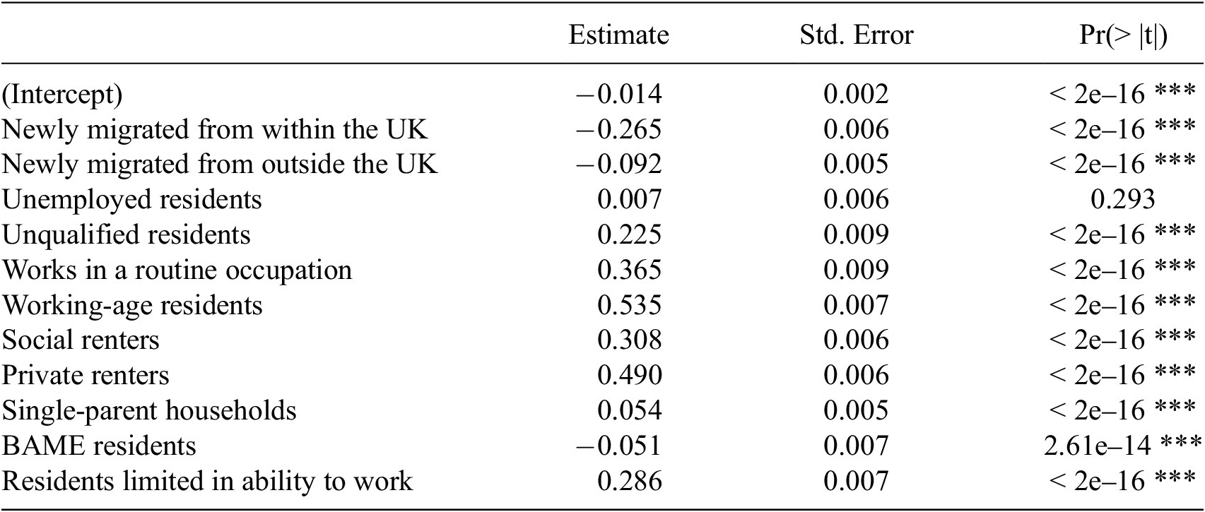
Of the key drivers identified, the largest group is employment-related. As a primary source of income for most of the population, the level and security of employment (if any) would be expected to have a sizeable influence on how able people are to pay any arrears and avoid finding themselves in the CCJ register (Dorling and Pritchard, Reference Dorling and Pritchard2010; Hiilamo, Reference Hiilamo2018). In line with this theory, a prevalence of lower-paid, less secure fields of work (modelled as routine occupations) leads to sizeable increases in expected standardised case rates (+0.365) within our model. A lack of qualifications in an area leads to a similar rise (+0.225), also reflecting the weaker, more precarious income streams (generally) available to this demographic. Increased proportions of a population being unable to work due to disability (temporary or permanent) leads to a comparable expected increase (+0.286) for similar reasons (Corlett, Reference Corlett2019; Guha, 2022). The most important driver (largest coefficient) in the model is the proportion of an LSOA’s population that is working-age, with a positive coefficient of 0.535. As noted previously (Jian Xiao and Yao, Reference Jian Xiao and Yao2014; Lawson et al., Reference Lawson, Lutzky, Kehoe and Gee2023), a lot of outstanding debt is concentrated within younger in-work demographics who are taking on debt early in their careers, expecting to pay it off later in life through (assumed) continuous wage growth (McCann, Reference McCann2013). This demographic is also much more likely to rent, which, as discussed in the following paragraph, has significant implications for CCJs and financial security in general. In contrast, the older retired population have generally settled many of their larger debts and have established for themselves some degree of financial security (Jian Xiao and Yao, Reference Jian Xiao and Yao2014). As “Working Age” population directly reflects the demographic that both earn and possess outstanding debts, the strong effect here is not at all surprising. Interestingly, unemployment was found to be insignificant in this initial model. Theory would suggest that unemployment would cause a rise in case rates, for the same reasons as lower income working, but we do not see this.

The composition of an LSOA’s housing market also has a significant impact on the model (+0.308 for social renters and + 0.490 for private). This is perhaps to be expected, with the majority of UK residents seeking financial advice at a major debt charity in 2022 living in rented properties (Stepchange, 2023). Within this, private renting is seen to have a greater impact on CCJ rates than social housing. Several prior studies have found that whilst private rent is almost always more expensive (Pateman and Richardson, Reference Pateman and Richardson2023), the household incomes and finances of privately renting tenants are often not (Bailey, Reference Bailey2020). Private accommodation is also generally seen as less secure, with less support from landlords when falling behind on payments and less legal recourse to protect tenant rights (Brickell and Nowicki, Reference Brickell and Nowicki2023; Stepchange, 2023), at least during the study period of this analysis. Housing quality (with regard to provisions such as insulation) is also often worse in low-income private tenancies. This can lead to increased costs for other potential debt obligations, such as utilities (Bailey, Reference Bailey2020; Brickell and Nowicki, Reference Brickell and Nowicki2023). Whilst private renting may have a larger coefficient, social renting also tends to house many individuals who face wider economic upheaval and challenges such as disability, homelessness and precarious/non-existent employment (Whitehead, Reference Whitehead, Scanlon and Fernadez Arrigoitia2014), which may be picked up by other modelled drivers. Finally, it is worth noting that in many cases renting and the previously discussed economic constraints intersect to trap residents. Rae (Reference Rae2015) found that many banks are hesitant to provide residents of poorer areas with mortgage loans, keeping them in riskier rental properties and potentially reliant on the unsecured options captured by the CCJ data.

Both single-parent households and minority groups have been identified across literature as being over-represented when looking at indebtedness (Simone and Walks, Reference Simone and Walks2019 and Brickell and Nowicki, Reference Brickell and Nowicki2023 are two respective examples). However, in our model both are found to have comparatively small effects, with a larger BAME population actually leading to slight decreases in case rates.

In the case of single parents, the reason for a surprisingly low effect may simply be that many of the reasons this group struggles with debt problems are tied to their economic position as a household unit. These drivers are already explicitly measured, so they are not picked up as a single-parent-exclusive effect. Nieuwenhuis and Maldonado (Reference Nieuwenhuis and Maldonado2018) found single parents are more likely to be in precarious low-paid work, and Brickell and Nowicki (Reference Brickell and Nowicki2023) note how rent arrears are a common challenge for single mothers, who are in general also over-represented in rental properties (Whitehead, Reference Whitehead, Scanlon and Fernadez Arrigoitia2014). These factors are already included separately as drivers in the model, and were found to lead to large increases in an area’s overall indebtedness. As such, areas with large single-parent populations are likely to experience high case rates even if the model does not appear to suggest this explicitly.

The reasons for non-white residents leading to a slight decrease (at odds with wider theory) in the model are potentially much more complex, and possibly a result of methodological limitations. Government data suggests that most ethnic groups are far more likely to live in the most deprived areas of the country. For example, Pakistani and Bangladeshi groups are three times more likely to live in an area in the bottom decile of overall and income-specific deprivation metrics than white British residents (UK Government, 2020). Furthermore, global debt discourse on “redlining” practices in the US against African Americans (Lang and Nakamura, Reference Lang and Nakamura1993; Hillier, Reference Hillier2003) means that much existing research (especially within North America) on race and debt observes systematic inequalities in debt ecosystems. Whilst race undoubtedly plays a role in many debt relations within the UK too, England and Wales do not immediately appear to see any such pattern at a scale comparable to redlining. Ultimately, the effect of race (or more accurately racism) as a “driver” of debt is not found to apply to the same extent on CCJ rates (Cowling et al., Reference Cowling, Liu and Conway2021). The reasons behind the slight decrease in case rates observed in areas with large minority populations across the UK are unclear. One possible partial explanation is due to differing cultural practices regarding loans and debts of many of the UK’s prominent ethnic minority demographics (Pollard and Samers, Reference Pollard and Samers2007). It is difficult to draw any concrete conclusions from this finding, however, as a blanket BAME category obscures many of the complex dynamics found within and between groups, and their consequent relationships with debt.

The final driver included in the model, migration, has been found to create pockets of higher debt in many other studies (Datta and Aznar, Reference Datta and Aznar2019; Simone and Walks, Reference Simone and Walks2019). However, in the case of CCJ rates, this does not appear to be the case. International migration’s impact is significant and negative but relatively small (−0.092), whilst internal movement was associated with a much larger decrease (−0.265). The likely explanation for this is simply that the migrants captured in the data have not resided in these areas long enough to have accumulated debts (e.g. rent arrears) sizeable enough to justify a CCJ. Considering said debts need to be processed by a relatively slow legal system and that migration data is measured relative to resident addresses only the year prior, this seems highly probable. It has also been argued that internal (economic) migration to urban areas reflects individuals/households with “higher human capital” seeking (better) employment (McCann, Reference McCann2013), or new labour market entrants such as students/recent graduates (commonly known as the escalator effect (Fielding, Reference Fielding1992). Neither of these demographics would be expected to be heavily over-indebted in the form captured by CCJs. The data estimates available do not distinguish between types of migrants, and it is probable that these broader factors obscure the debt challenges identified in previous debt literature.

4.4. Model residuals

The model presented in Table 2 captures most (%), but not all of the spatial variation in CCJ rates. From Figure 3, it is clear that the model accuracy decreases in LSOAs with the lowest case rates, overpredicting for many of the areas without many CCJs per capita. A Moran’s I analysis of the residuals returns a value of 0.213 (p-value: 0.001), implying at least some spatial pattern to the residuals. As most of the model error is found in areas at the extremes of case rates (which are already found in 1b to be strongly spatially clustered), this is expected. Section 4.5 deals with addressing this spatial aspect through further models.

Table 2.

OLS regression coefficients

Table 2. Long description

Columns include: Variable names, coefficent estimate, standard error, p-value (for significance check). Specific values are presented in the accompanying text.

Note: *** denotes significance to the 0.001 level, ** the 0.01 level, and * the 0.05 level.

Figure 3.

Model residuals across CCJ case rate deciles.

Figure 3. Long description

A boxplot with 10 “CCJ rate decile” categories along the x-axis and “OLS model residual” scales continuously from −1.5 to 2.5 on the y-axis. A red horizontal line intercepts the y-axis at 0. The results show that for all but the lowest case rate decile the median residual is close to 0. In the bottom decile, the majority of areas saw case rates over-estimated.

4.5. Spatial lag and mixed-effects

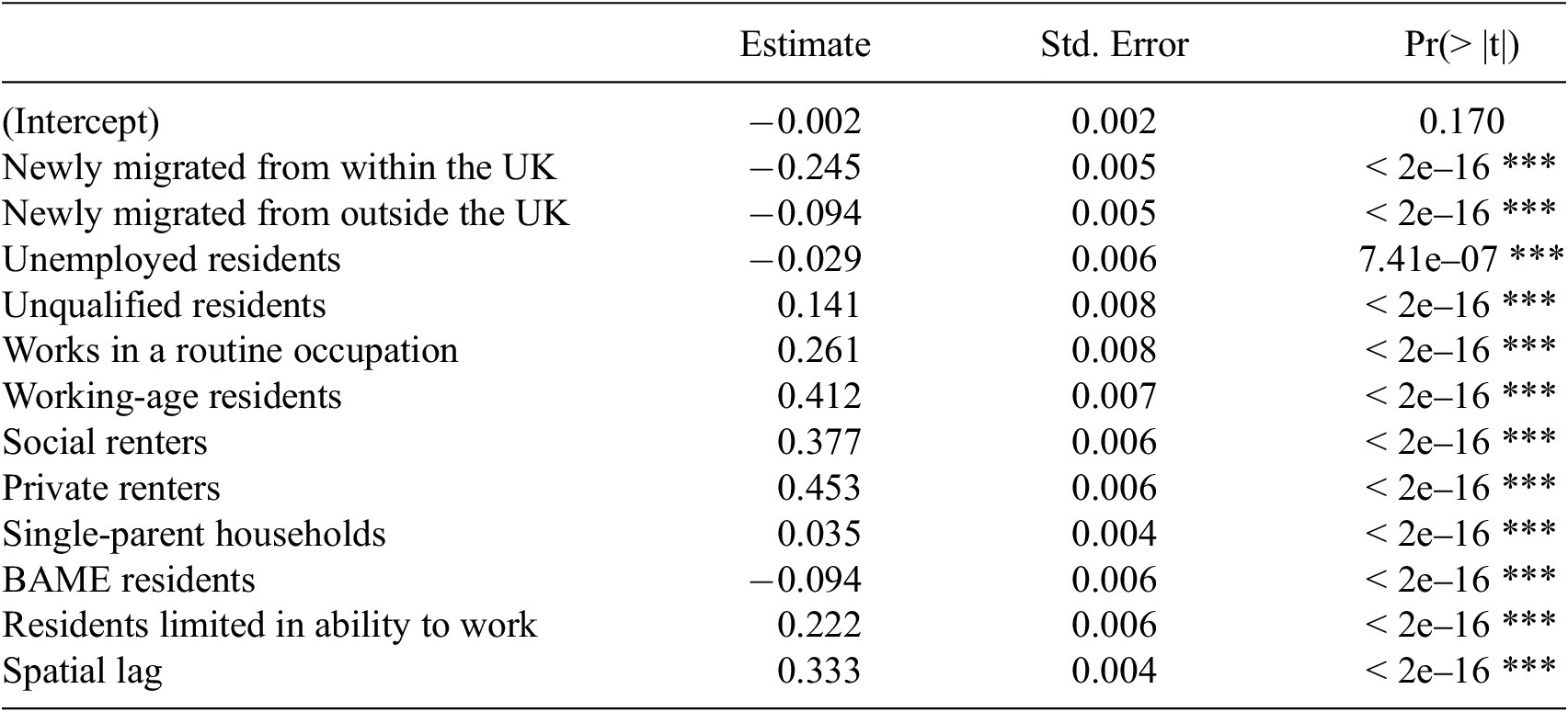
As seen in Figure 1b, CCJ rates have a clear pattern of spatial autocorrelation. Therefore, it makes sense to include this effect in the model, measuring whether being surrounded by high case rates also raises expected CCJ rates in an LSOA. This was done through the addition of spatial lag as a coefficient, the results of which can be seen below in Table 3.

Table 3.

Spatial lag model

Table 3. Long description

Table is almost identical to table 2, with the additional row measuring the effect of spatial lag. Columns include: Variable names, coefficent estimate, standard error, p-value (for significance check). Specific values are presented in the accompanying text.

The addition of a lag effect improved the model further, raising the R² = 0.827, and shows a strong positive coefficient (+0.333). This suggests that even after accounting for the various included drivers, being in an area surrounded by high case rates further increases the expected CCJ rate. This likely reflects the spatial concentration of other unidentified drivers across these high-rate areas. The coefficients of the drivers did not change drastically, though of note unemployment became significant (though the coefficient remains small) and the size of the working-age resident coefficient dropped below that of private renting. Despite the model improvement, even after accounting for this lag, a spatial element to residuals persists (Moran’s I = 0.126, p-value = 0.001).

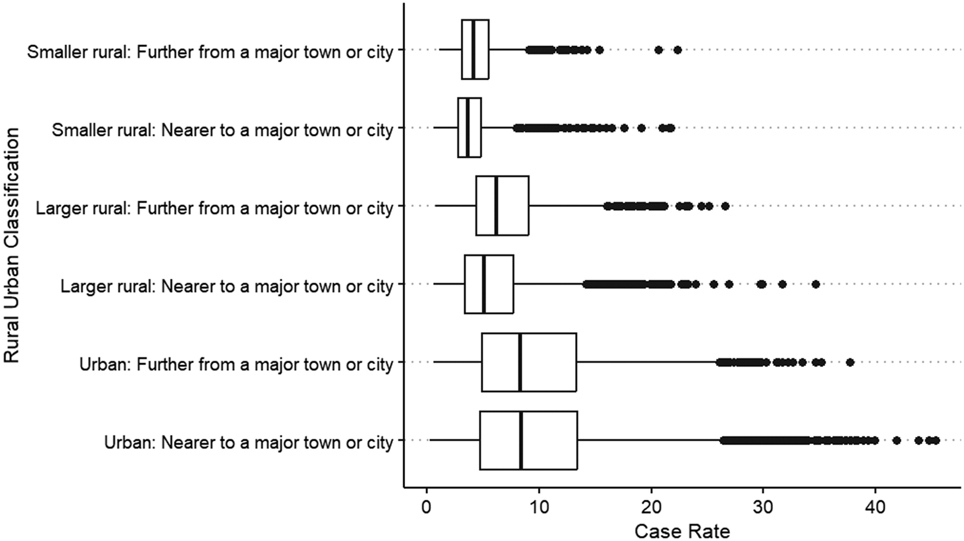
Looking at the initial distributions in Figure 1, another potential spatial pattern to address is the different levels of urbanisation. When RUCs are used to group the LSOAs, a large range can be seen in each category (Figure 4). In general, however, the more urban areas do have higher case rates on average, and also experience the highest case rates seen anywhere in the dataset. This is in line with wider theory, with Glaeser and Gyourko (Reference Glaeser and Gyourko2005) identifying clear patterns of cities in decline attracting large income-deprived populations (due to the reduced housing costs in these areas, which, as already discussed, is a major concern for many facing over-indebtedness). Also of note is that there is a much wider spread in these urban areas, perhaps reflecting the large variation in forms of urban living, with both very financially secure and distressed populations residing within these areas.

Figure 4.

Case rates across rural-urban classification groups.

Figure 4. Long description

A horizontal box plot graph where the categorical y-axis groups each rural-urban classification. The x-axis is a continuous scale of CCJ case rate. The plot shows median case rate was under 10 for all areas, but that more urban areas have larger tails in the higher case rate direction.

Despite these patterns, adding RUC to the regression did not meaningfully improve our results (R² increased from 0.8270 to 0.8271). RUC was still found to have a significant effect, with increasing levels of urbanisation showing increasing (though very small) coefficients compared to the reference group of most rural areas (see Appendix B, Table B1 for the full coefficient table). Figure 5 shows the resultant residuals of this third model. Overall, residuals were mostly minimal across all areas (in line with the overall high accuracy), though there are several instances of severe over- and under-predictions in the urban areas. This is likely a result of the wide spread of values seen in the initial case rates (Figure 4), with many of the dataset’s largest outliers (in both directions) being found in urban LSOAs. As discussed above, the concentrating of financially vulnerable groups into urban areas follows well-understood economic patterns (Glaeser and Gyourko, Reference Glaeser and Gyourko2005; McCann, Reference McCann2013). This not only explains the case rate’s spatial distribution generally, but also perhaps why RUC has only a limited effect. If much of the clustering seen in urban areas is down to economic and housing factors, this is already accounted for in the model’s variables, and so will not be picked up as a specific Rural-Urban effect.

Figure 5.

RUC mixed-effects model residuals.

Figure 5. Long description

A horizontal box plot graph with Rural-Urban classifications on the y-axis (the same as figure 4), and residuals on the x-axis (a continuous scale ranging from −30 to 30. A vertical line coloured red intersects the x-axis at 0. For all groups, the 25th to 75th percentiles of errors were very close to 0. As with figure 4, the more urban areas saw larger tails and more outliers, this time in both direction.

When the data was instead grouped to each parent MSOA (Office for National Statistics, 2021), the R² value increased notably, from 0.82 to 0.87. As the coefficients themselves did not change significantly (see Appendix B, Table B2), this supports concerns that there is still a spatial aspect to the patterns of CCJ rates beyond the included drivers. A Moran’s I analysis of this new model’s residuals returns a statistically insignificant value of −0.045 (p-value: 0.999). This result suggests that around half of the variation not covered by the original model was also due to factors that vary spatially, this time at the MSOA level. What these specific factors are remains unclear and is a potential avenue for further research.

4.6. Regional differences in driver coefficients

As a final point of discussion on the role space plays in driving indebtedness, a comparison of separate spatial lag models for Wales, London and the rest of England is presented. Whilst Section 4.5 has shown that there is a) a significant amount of spatial variation in case rates, and b) a significant spatial aspect to the concentrations of the key drivers of over-indebtedness, it does not discuss how the relationship between these two distributions can also change. The three models below show this to be very much the case (Table 4).

Table 4.

Regional spatial lag models

Table 4. Long description

Variables remain the same as in Table 3, as do columns. However, the coefficients, standard error and p-value columns are each repeated 3 times (one for London, one for the rest of England and one for Wales).

All three models performed well, with R² values comparable to the original lagged model (0.794 for London, 0.832 for the rest of England, and 0.858 for Wales). Large discrepancies in coefficients between regions can be observed, though in most cases the overall trends persist (renting, working-age and routine occupation continue to dominate, but to varying amounts). Some of the more striking variations, however, are discussed below.

The negative coefficient assigned to BAME populations in the first model is clearly a product entirely borne of LSOAs in the “rest of England” group, with both Wales and London seeing areas dominated by these demographics experience the originally expected higher case rates. The shared change to a positive effect (though very small in London) is surprising. Compared to the rest of England, Wales has a relatively small ethnic minority population, whilst London’s is drastically larger (UK Government, 2022). As discussed earlier, unpacking the effect of this group is difficult due to the wide range of backgrounds and circumstances it represents, and so any findings should be treated with appropriate caution. However, the positive coefficient for Wales is potentially due to the largest non-white populations being incredibly spatially concentrated into a very low number of highly deprived urban area LSOAs, all of which experience relatively high case rates. London, on the other hand, is a much more ethnically heterogeneous area compared to both wider England and to Wales. The reduction in ethnicity coefficients seen here may simply be a reflection of a more mixed population not seeing these concentrated pockets of deprived ethnic minorities to quite the same extent as other parts of the country.

Another interesting finding is that the size of the qualification level coefficient is noticeably reduced in London, and completely insignificant in Wales. Alongside this, routine occupations have a much larger positive effect in both these regions compared to the rest of England. In London’s case, low-income work does not provide significantly more in wages than elsewhere in the country despite policy measures such as the London living wage (London City Hall, 2026), whilst living costs are higher (McCann, Reference McCann2013; Edwards, Reference Edwards2016). This inevitably leads to more financial insecurity for those working in these occupations. In Wales’ case, the highest routine occupation concentrations are almost entirely in the South Valleys, which, as discussed in the descriptive analysis, is a major hotspot for CCJs.

4.7. Limitations and possible explanations for remaining variation

As noted previously, there is no agreed-upon single definition for over-indebtedness (D’Alessio and Iezzi, Reference D’Alessio and Iezzi2013), and whilst there have been attempts to unify the many distinctions into a singular catch-all definition, there remain notable variations at both international/governmental levels (Davydoff et al., Reference Davydoff, Dessart, Naacke, Jentzsch, Figueira, Rothemund, Mueller, Kempson, Atkinson, Finney and Anderloni2008) and within academia (Cesar Leandro and Botelho, Reference Cesar Leandro and Botelho2022). Focusing on our specific dataset, the annual record counts of the GeoDS dataset used do not fully align with official Registry Trust statistics, underrepresenting case counts within each year. We do not believe this discrepancy causes any biases in the data or findings, but it is still worth noting. A more pressing concern is that the time period available to study, 2016–2023, features heavy disruptions to the court system due to COVID-19. This means cases were not being processed at usual rates and therefore the case counts probably underestimate true instances of over-indebtedness. Despite these caveats, the spatial distribution of the CCJ rates measured (shown in Figure 1a) do still align with other, wider lensed, metrics of unsecured debt (such as those shown by Hutchison et al., Reference Hutchison, Tiwari, Koblyakova, Green and Tan2024 and Lowell, 2024), supporting our argument that this dataset is a fair representation of (relative) indebtedness patterns across England and Wales. Ultimately, CCJs reflect what is often a last case scenario, where creditors see legal action as the only viable move remaining. This would explain why they are far less frequent in volume than other self-reported measurements of debt.

Though extensive, the initial list of debt drivers used was not exhaustive. With debt being such a consistent source of academic discussion, it has been ascribed to too many demographic characteristics to feasibly include here. Wherever possible, prominent characteristics were included, but several were excluded due to a lack of high-quality data available to measure them at the resolutions studied. For example, there are many individual factors that influence debt accumulation and management, such as financial literacy (James, Reference James2022), which we were unable to satisfactorily reflect with data at the LSOA level. Evidence of this can be seen in the MSOA-level model, which identified the effect of further, unidentified, spatially varied drivers. Finally, the regional models show that the drivers identified here are likely not universal and can already be seen to vary in impact within a single nation. Whilst this does not diminish their importance, it does highlight the need for further research when looking beyond the study region presented.

Despite all of these caveats, it should be stated that the models performed very well and could not only identify the areas at highest risk of receiving CCJs with great accuracy but also explain the majority of variation in the specific case rate values.