The Reliable Change Index

In their seminal paper on the reliable change index, Jacobson, Follette and Revenstorf (Reference Jacobson, Follette and Revenstorf1984, p. 339) wrote: ‘We believe that the field [of psychotherapeutic intervention] needs agreed-upon conventions for determining what constitutes improvement in an individual, and, if possible, general consensus as to what is meant by clinical significance’. At the time, criteria for what constituted improvement were unspecified, qualitative or, at best, arbitrary.

They proposed a twofold empirical criterion for determining whether or not real improvement had occurred during the course of therapy. First, there had to be a clinically significant change, such that scores on the measure used to evaluate the therapy moved from dysfunctional to the functional range during the course of therapy. Assuming normal distributions for the functional and dysfunctional populations, they proposed three cut-off points, differing in stringency, for determining clinical significance – crossing over from the dysfunctional to the functional range. Second, the magnitude of change in scores also had to be statistically significant (i.e., reliable) and due to real change, not attributable to measurement error. They proposed a reliable change index (RCI) to determine the reliability of a change in scores. In order to address criticisms of their original formula for the RCI, it was subsequently modified to ${\rm RC} = \left( {x_2 - x_1 } \right)/\delta *\sqrt {2\left( {1 - r_{12} } \right)} $, (Jacobson & Truax, Reference Jacobson and Truax1991), where x ₁ is the test score at time 1, x ₂ is the test score at time 2, δ is the standard deviation of the test, and r ₁₂ is the test–retest reliability.

The determination of clinically significant change and calculation of reliable change were first illustrated in the paper using hypothetical data, which was not specified as being ordinal, interval or ratio. Later on in the paper, pre–post scores on the Dyadic Adjustment Scale (DAS) for couples receiving behavioural marital therapy were used to illustrate clinical significance and reliable change after therapy. From the graph used to display the data, it is evident that a change of approximately 12 points on the DAS is needed for the change to be reliable at the .05 level. Given that the DAS is an ordinal scale, the question is: is a difference of 12 points the same all along the scale range? The issue is not raised in the paper or in Jacobson's subsequent papers on the subject (e.g., Jacobson, Follette, & Revenstorf, Reference Jacobson, Follette and Revenstorf1986; Jacobson, Roberts, Berns, & McGlinchey, Reference Jacobson, Roberts, Berns and McGlinchey1999; Jacobson & Truax, Reference Jacobson and Truax1991). Indeed, although there has been much discussion about the RCI in the literature over the years, and multiple refinements have been proposed to address statistical and theoretical shortcomings of the original formulation (for example, see Chelune, Naugle, Luders, Seldak, & Awad, Reference Chelune, Naugle, Luders, Seldak and Awad1993; Christensen & Mendoza, Reference Christensen and Mendoza1986; Collie, Maruff, McStephen, & Darby, Reference Collie, Maruff, McStephen and Darby2003; Hageman & Arrindell, Reference Hageman and Arrindell1993; Iverson, Reference Iverson2001; Maassen, Reference Maassen2004), its appropriateness when used with ordinal-scale data has not been given consideration. Given that many of the scales used in behavioural research and clinical work are ordinal scales, this is an important issue.

Scales of Measurement

Stevens (Reference Stevens1946) argued that there are different classes of scales of measurement (namely, nominal ordinal, interval and ratio) that:

For the purpose of this paper, briefly discussing the properties of ordinal and interval scales will suffice. According to Stevens, each type of scale embodies specific empirical operations, and only certain transformations which leave the scale form invariant are permissible for each type. Ordinal scales determine only rank-order and ‘the linearity of an ordinal scale is precisely the property which is open to question’ (Stevens, Reference Stevens1946, p. 679). The only permissible transformation consists of transformations by monotonic functions (i.e., functions which either increase or decrease monotonically) whereby the order between ordered sets is preserved. That is, the order of items in the ‘original’ and the transformed scale is the same. Stevens argues that means and standard deviations should not be used with ordinal scales because ‘these statistics imply a knowledge of something more than the relative rank-order of data’ (Stevens, Reference Stevens1946, p. 679).

Interval scales determine the equality of intervals or differences between values. Linear transformations (e.g., y = ax + b) are permissible with this scale, such that the linear relationship between any two pairs of values in the original and transformed scale remains the same. For example, there is the same difference in temperature between 10 and 20 degrees, and between 40 and 50 degrees in the Celsius scale. These relationships are maintained if temperatures are converted from Celsius to the Fahrenheit scale (F° = 1.8*C° + 32). For these reasons, descriptive statistics such as means and standard deviations are applicable to interval-scale data, and parametric statistics are permissible.

The Controversy

Since Stevens published his paper, there has been spirited debate about whether or not parametric statistical analyses can be used legitimately with ordinal-scale data. Although a comprehensive appraisal of the controversy is beyond the scope of this paper, a brief overview is in order (for a detailed discussion, see Knapp, Reference Knapp1990; Labovitz, Reference Labovitz1972; Norman, Reference Norman2010; Nunnally, Reference Nunnally1975). Nunnally (Reference Nunnally1975) identified three camps: those who strictly proscribed the use of parametric statistics with ordinal data, let's call them the purists; those who mounted statistical arguments and cited empirical evidence supporting the permissibility of using parametric techniques with ordinal data, let's call them the dissenters; and a silent majority who ignored the debate and went on using parametric techniques. Kuzon, Urbanchek and McCabe (Reference Kuzon, Urbanchek and McCabe1996) clearly belong in the purist camp. They considered the use of parametric methods to analyse ordinal data, the first of the seven deadly sins of statistical analysis. They argued that arithmetical operations involved in the computation of population parameters and sample statistics, such as means, standard deviation and variance, are not valid when used on numerical variables representing verbal statements that only indicate unquantified relative differences (e.g., agree vs. strongly agree). They illustrate their argument by suggesting that the average of a scale consisting of the rankings 1 = poor, 2 = fair, 3 = good and 4 = excellent is not ‘fair and a half’ (where as the average of 1, 2, 3 and 4 is 2.5). Others (e.g., Vigderhous, Reference Vigderhous1977) demonstrated that building regression models (partial correlations) for ordinal data using parametric or non-parametric methods can yield different results and, consequently, different inferences will be made about the data depending on the method of analysis used.

However, this camp is often criticised by the dissenters for: (i) basing the proscription of analysis of ordinal data with parametric statistics on arguments based on measurement theory, not on statistical theory; and (ii) not taking note of the strong empirical evidence that suggests that it is permissible to use parametric statistics with ordinal data. With respect to the first criticism, Carifio and Perla (Reference Carifio and Perla2007) reviewed empirical evidence supporting the contention that while individual items in rating scales are ordinal in nature (essentially Likert scales), total-scale scores (made up of many individual items) produce empirically interval-scale data (for example, see Carifio, Reference Carifio1978; Vickers, Reference Vickers1999). Norman (Reference Norman2010) further argues that while not knowing the true ‘distance’ between levels in an ordinal scale precludes making inferences about the latent construct being measured, this is irrelevant and does not proscribe the use of parametric analysis. He argues that if the data have a reasonable distribution, then parametric techniques may be used to make valid inferences about means, differences in scores and so forth.

With respect to the second criticism, there is strong evidence to support the contention that the assumptions underlying parametric analysis can tolerate violations quite well. For example, using Monte Carlo simulations, Glass, Peckham and Sanders (Reference Glass, Peckham and Sanders1972) showed convincingly that except for extreme violations of the homoscedasticity assumption (homogeneity of variance), the F test is extremely robust to violations of other basic assumptions and can be validly used to analyse ordinal data. Lucke (Reference Lucke1996) used Monte Carlo simulations to examine the distribution of the t-test statistic when comparing two independent samples on the Glasgow Coma Scale. He found that t-tests produced Type I error rates not exceeding predetermined levels of significance when group size was at least 30. More recently, Murray (Reference Murray2013) used data from a sample of 111 university students to compare the results of using parametric and non-parametric correlations on ordinal data. She calculated point-biserial correlations between four constructs (mathematics self-efficacy, academic self-regulation, availability of academic resources and learning styles) and found that while Pearson's r and Spearman's rho produced the same results for all variables, analyses using Kendall's tau_b, produced different results on some variables.

Is the RCI Meaningful with Ordinal Data?

The RCI is used to determine whether or not the distance between scores – two points in a scale – is due to real change (i.e., statistically significant) or due to measurement error. If calculation of the RCI indicates that a score difference of, say, 15 points constitutes a reliable change, this criterion is applied to scores anywhere on the range of test scores. With interval- or ratio-scale data, this makes sense because a difference of 15 points is the same all along the range of test scores. That is, the difference between, say, 6 and 21 is the same as that between 21 and 36. This is not the case for ordinal-scale data. Consider the ratings for Item 10 (crying) of the revised Beck Depression Inventory (BDI-II; Beck, Steer, & Brown, Reference Beck, Steer and Brown1996): 0 = I don't cry any more than I used to; 1 = I cry more than I used to; 2 = I cry over every little thing; 3 = I feel like crying but I can’t. Numerically, the difference between a rating of, say, 1 and a rating of 2 on this item is the same as that between a rating of 2 and a rating of 3. By contrast, the real difference between these two pairs of ratings in terms of the underlying construct being measured is somewhat a matter of conjecture.

Stevens (Reference Stevens1946, p. 679) argued that ‘means and standard deviations computed on an ordinal scale are in error to the extent that the successive intervals on the scale are unequal in size’. Given that δ (standard deviation) is used in the computation of RCI, is it appropriate to use this statistic when dealing with ordinal data? How reliable are the conclusions that can be drawn about changes in test–retest scores when the RCI is computed for ordinal-scale data? In the following sections, real data from the Sydney Psychosocial Reintegration Scale – Version 2 (SPRS-2; Tate, Reference Tate2011) will be used to explore this question and illustrate how the RCI ‘performs’ when applied to ordinal-scale data, and, in particular, how it ‘performs’ across the range of scores in the data.

An Illustrated Example

The SPRS-2 is a 12-item rating scale that measures an individual's level of participation in three domains following traumatic brain injury (TBI): occupational, interpersonal relationships and independent living skills. Two forms are available and items in each form are rated on a five-point Likert scale. Form A measures change since injury, with ratings ranging from 0 (extreme change) to 4 (no change at all). Form B measures current status, with ratings ranging from 0 (extremely poor) to 4 (very good). Total Raw Scores on each Form range from 0 to 48, with higher scores indicating a better level of function.

Tate, Simpson, Soo and Lane-Brown (Reference Tate, Simpson, Soo and Lane-Brown2011) explored the psychometric properties of the SPRS-2 and reported levels of function in two samples of participants with TBI living in the community. Form A (change since injury) was administered to 201 individuals and Form B (current status) to 150 individuals. In addition, Rasch analysis was performed on the raw data of both TBI groups, and Tate and colleagues provide a table for converting raw scores to logit scores. The Rasch model does not, strictly speaking, convert an ordinal scale into an interval scale, but rather constructs linear measures from counts of qualitatively ordered observations (Salzberger, Reference Salzberger2010). Thus, Rasch logit scores provide data akin to interval-scale data, for which it is valid to calculate means and standard deviations. The SPRS-2 was chosen for this demonstration because it is one of the few rating scales for which both raw scores and Rasch data are available. Hence, an RCI derived from both types of data can be calculated and the way in which each RCI classifies test–retest differences along the range of Total Raw Scores can be compared.

Given that Form B can be re-administered to determine whether or not a change in level of activity has occurred over time, both raw and logit scores for the 150 TBI participants who completed this form will be used. The RCI for α = .05 (one tailed) will be computed using raw and logit scores. Transposing the formula and solving for x ₂ − x ₁ will yield the minimum reliable difference (MRD) that is needed between test–retest scores in order for a reliable change to have occurred (see Table 1). Calculation of the reliable change criteria in terms of raw scores (MRD_RS) and in terms of logit scores (MDR_LS) is also shown in Table 1. The Form B sample statistics used in these calculations were derived from the psychometric study of Tate et al. (Reference Tate, Simpson, Soo and Lane-Brown2011): standard deviation of raw scores (σ_RS) = 12.5; standard deviation of logit scores (σ_LS) = 15.54; test–retest reliability (ICC) = .90. The same ICC for test–retest reliability was assumed to be applicable to both raw and logit scores.

TABLE 1

Derivation of the Minimum Reliable Difference (MRD) Formula and Calculation of Reliable Difference Criteria for Raw Scores (MRD_RS) and Logit Scores (MRD_LS) – Form B of the SPRS-2

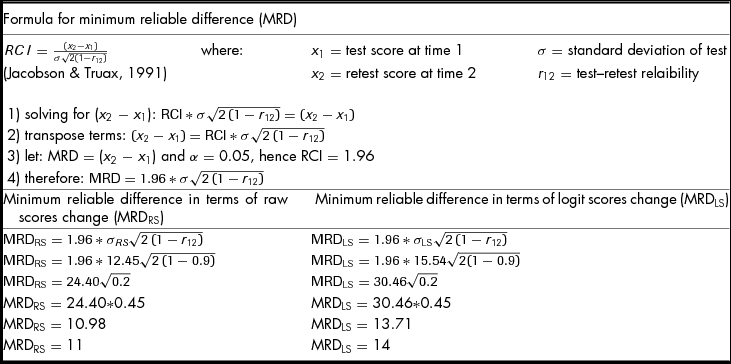
Sample = 150 patients with TBI; σ_RS = 12.45, standard deviation of raw scores; σ_LS = 15.54 standard deviation of logit scores; ICC = .9, α = .05, one tailed, corresponding to z-score = 1.96.

As Table 1 shows, raw scores and logit scores produce quite different criteria for reliable change: MRD_RS = 11 for raw scores, and MRD_LS = 14 for logit scores. This difference exclusively reflects the difference in the standard deviation of each data set, which in itself indicates that the distribution of raw and logit scores is different. But, how comparable is the determination of reliable test–retest differences when MRD_RS and MRD_LS are used?

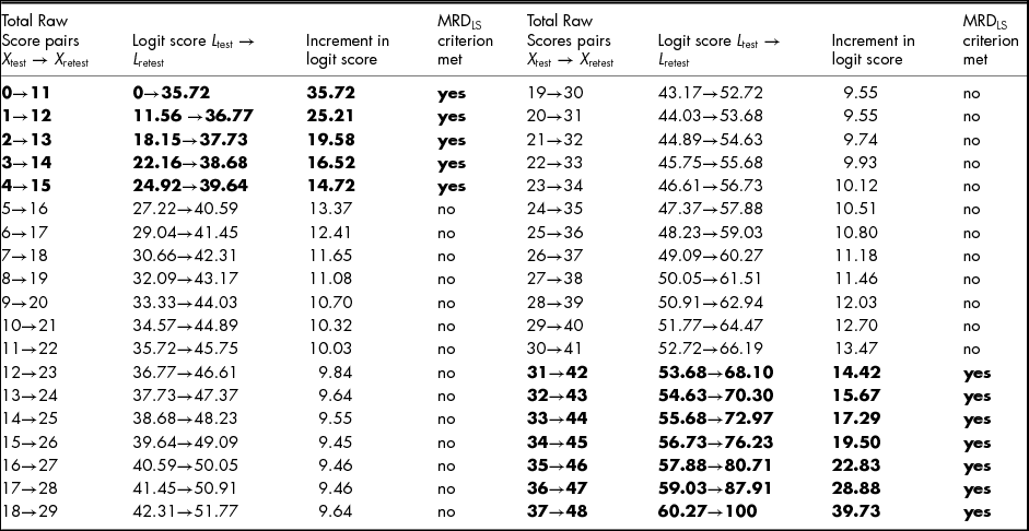
Comparison of the raw score criteria for reliable change (MRD_RS) against the logit score criteria for reliable change (MDR_LS) is shown in Table 2. Increments in raw scores across the range were set to be reliable according to the MRD_RS criterion and then evaluated with the MRD_LS criterion. Starting with the lowest SPRS-2 Total Raw Score (i.e., 0) the first column in Table 2 (Total Raw Score pairs X _test → X _retest) shows raw scores pairs across the range of Total Raw Scores that are deemed to be reliably different according to the MRD_RS criterion (i.e., a difference of 11 points). Column two (logit score L _test → L _retest) shows the raw score pairs in the first column converted to logit scores. The third column (increment in logit score) shows the difference between the logit scores in column two. Finally, the fourth column (MRD_LS) shows whether or not the difference in logit scores meets the MRD_LS criterion for reliability (i.e., a difference of 14 points). For example, the third row of the table shows an initial raw score of 2 (X _test) increasing to 13 (X _retest), a difference of 11 points which, according to the MRD_RS calculated earlier, is reliable. The corresponding logit scores for these raw scores are 18.5 (L _test) and 37.73 (L _retest), a difference of 19.58 logit points, which, according to the MRD_LS calculated earlier, is also reliable.

TABLE 2

Comparison of MRD_RS against MRD_LS: Raw Scores Differences across SPRS-2 Total Raw Score Range that meet MRD_RS Criterion for Reliable Change, Equivalent Differences in Logit Scores and Determination of Reliable Change According to MRD_LS Criterion

X _test = Raw score at time 1; X _retest = raw score at time 2; L _test = logit score at time 1; L _retest = logit score at time 2. Bold entries indicate concordance between MRD_RS and MRD_LS criteria.

Differences between all raw score pairs shown in column one of Table 2 were deliberately chosen to be reliable in terms of raw score points according to the MRD_RS criterion. As can be seen in Table 2, at either end of the Total Raw Score distribution the increments in raw scores are also deemed to be reliable according to the MRD_LS criterion, just as in the example above. However, as shown in the fifth row of Table 2, a raw score increase from 5 to 16, corresponds to a logit score increase of 13.37 points, which is not reliable according to the MRD_LS criterion. The discrepancy between the raw-score-derived and logit-score-derived reliability criteria occurs throughout most of the central section of the Total Raw Score range. When initial raw scores fall between 5 and 30, reliable increments in terms of the MRD_RS criterion are not deemed to be reliable in terms of the MRD_LS criterion. Concordance between the two criteria only occurs at the extremes of the Total Raw Score range.

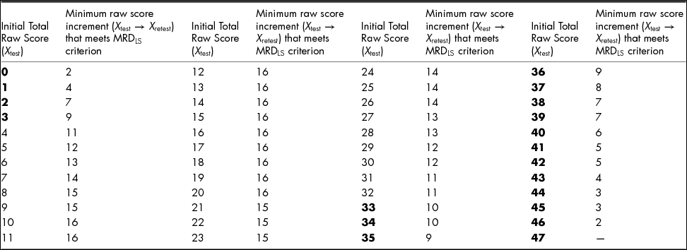
Table 3 looks at these data from a different perspective. In this instance the aim was to determine the minimum number of points an initial raw score needs to increase in order to meet the MDR_LS criterion for reliability. The first column in Table 3 shows initial raw scores (X _test) across the Total Raw Score range. The second column shows the minimum increment required in order for the change in raw score to be deemed reliable according to the MRD_LS criterion.

TABLE 3

Determination of the Minimum Increment in Raw Scores (X _test → X _retest) needed to meet MRD_LS Criterion for Reliable Change

Bold numbers indicate initial raw scores (X _test) that need to increase less than 11 points (i.e., MRD_RS criterion for reliable change) in order to meet the MRD_LS criterion for reliable change (i.e., a difference of 14 points).

For instance, with an initial raw score of 0, an increment of only 1 point, from 0 to 1, is equivalent to an 11.56 point change in terms of the logit score metric, which is not reliable according to the MRD_LS criterion. By contrast, as Table 3 shows, an increment in of 2 points, from 0 to 3, which is equivalent to an 18.15 point change in terms of the logit score metric, is reliable according to the MRD_LS criterion. The minimum increment in raw score points needed to meet the MDR_LS criterion for reliability is small at the beginning of the total raw score distribution (i.e., 2), then increases steadily, stabilising between 14 and 16 points in the centre of the distribution, then begins to decrease steadily, reverting to very low values at the upper end of the distribution (i.e., 2).

As Table 3 shows, if the initial raw score falls between 0 and 3 or between 33 and 46, an increment of less than 11 raw score points (i.e., the MRD_RS criterion) results in a change that is deemed reliable according to the MRD_LS criterion. Thus, relatively smaller raw score increments at the extremes than at the centre of the Total Raw Score range produce changes that are deemed to be reliable according to a metric that provides a linear measure of the raw data, namely logit scores. Conversely, small changes in raw scores at either end of the Total Raw Score range are deemed to be unreliable if a criterion derived from ordinal, namely MRD_RS, is used.

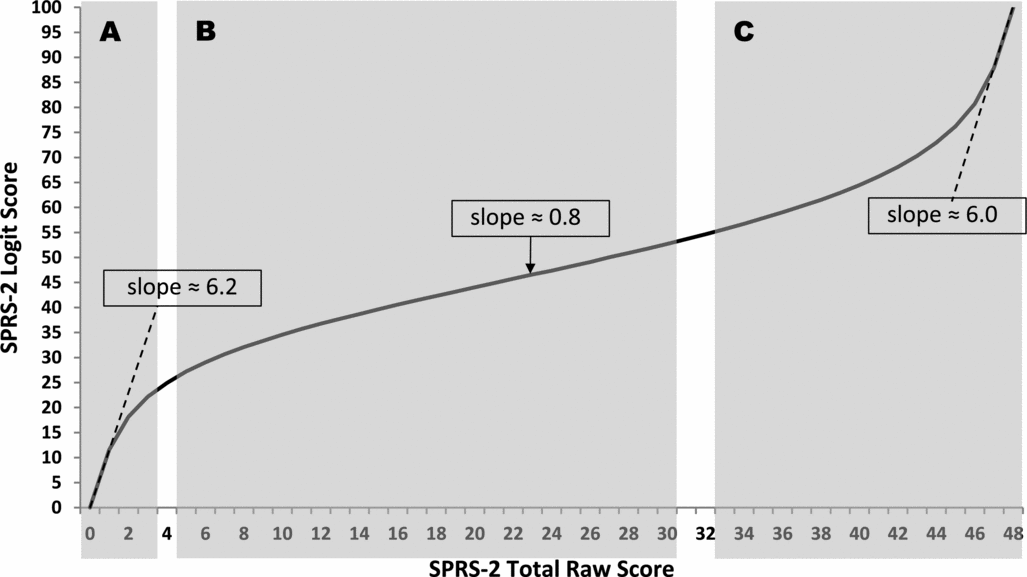
The discrepancies demonstrated in Tables 2 and 3 indicate that across their range, raw scores derived from an ordinal scale of measurement do not map evenly on to a linear metric. These discrepancies are clearly demonstrated in Figure 1. Total Raw SPRS-2 Scores are shown on the horizontal axis in the graph and logit scores are shown on the vertical axis. The graph shows the correspondence between raw and logit scores (plotted from the raw-to-logit score conversion table reported in Tate et al., Reference Tate, Simpson, Soo and Lane-Brown2011).

FIGURE 1

Correspondence between SPRS-2 raw scores and logit scores derived from Rasch analysis.

As Figure 1 shows, the slope of the graph is relatively steep at the lower and upper extremes of the Total Raw Score range (approximately 6.2 and 6.0, respectively), and considerably flatter in the centre of the range (approximately 0.8). That is, as Total Raw Score increases, the rate of increment in logit score at the extreme ends of the range is approximately seven times larger than in the centre of the range. Given that logit scores are linearly distributed and uniformly spaced, the difference in slopes across the graph illustrates that the distance between consecutive raw scores is greater at extremes than in the centre of the Total Raw Score distribution. Given that the raison d’être of the RCI is to determine whether or not changes over time in the construct being measured are significant, then uniformity in the distance between consecutive raw scores across the whole Total Raw Score range is crucial. Otherwise, the MRD_RS can yield erroneous conclusions, depending on where the test–retest difference being evaluated is situated on the Total Raw Score range.

The discrepancies between MRD_RS and MRD_LS revealed in Tables 2 and 3 can be graphically illustrated as follows. If the initial Total Raw Score is within shaded areas A or C of Figure 1, less than the 11-point increment required for a reliable change in terms of the MRD_RS criterion produces a reliable change in terms of the MRD_LS criterion. If the initial Total Raw Score is in shaded area B, an 11-point increment required to meet the MRD_RS criterion, does not meet the MRD_LS criterion. If the initial Total Raw Score is 4, 31 or 32, an 11-point increment required for the MRD_RS criterion also meets the MRD_LS criterion.