2.1. Real-time timbre recognition

Timbre is now available as a control structure for real-time electroacoustic music. Early work in this area was done by Lippe (Reference Lippe1993) using Max and the IRCAM Signal Processing Workstation (ISPW) to analyse timbre in performance.

More recently, Hsu (Reference Hsu2006) used real-time timbre recognition of the saxophone to guide an interactive system. Ciufo (Reference Ciufo2005) used Jehan and Schoner (Reference Jehan and Schoner2001) to analyse incoming audio, which in turn influenced processing. Similarly, Rebelo and Renaud (Reference Rebelo and Renaud2006) used the same software in the BLISS laptop improvisation ensemble to analyse ensemble members’ spectral data, providing information that was shared amongst the ensemble. These open-source real-time analysis tools written for Max/MSP allow composers to explore the potential of timbre as a control element during performance within a widely used software environment. Furthermore, the addition of the Small Music Information Retrieval Toolkit (Fiebrink, Wang and Cook Reference Fiebrink, Wang and Cook2008) to ChucK will, no doubt, precipitate many new real-time works that involve timbral recognition, previously only possible using non-real-time tools.

2.2. Timbre organisation

The Music Information Retrieval (MIR) community has done considerable research into timbral organisation, specifically in determining similarity between songs (Tzanetakis and Cook Reference Tzanetakis and Cook2000). Cano and Koppenberger (Reference Cano and Koppenberger2004) describe a system that classifies a huge sound-effects database, discovers timbral similarities between sounds, and labels these sounds with metadata tags. Pampalk, Dixon and Widmer (Reference Pampalk, Dixon and Widmer2004) describe a system which combines descriptors derived from audio analysis with meta-information to create different views of a music collection, using an aligned SOM. This builds upon work by Logan (Reference Logan2002), who uses a spectrum-based similarity measure to create playlists of similar songs, and Aucouturier and Pachet (Reference Aucouturier and Pachet2002), who use a spectrum-based similarity measure to find similarities between songs. Lübbers (Reference Lübbers2005) describes a system called ‘The Sonic SOM’, which uses a SOM to help users understand their music collections. Knees (Knees, Pohle, Schedl and Widmer Reference Knees, Pohle, Schedl and Widmer2006) presents another system that uses text-retrieval methods to find meta-data extracted from the Web in order to discover song similarities.

2.3. Differences from previous work

The work described here focuses upon real-time selection of samples based on their timbral features, and is thus different from most previous timbral analysis research. Furthermore, it does not use meta-data to organise databases, allowing for greater flexibility.

As the authors are both composers, the intentions are also markedly different from MIR research: rather than attempting to navigate a search space and return an exact match, the interest is in discovering similar timbres. For example, in cases where the software is used to select timbres based on live input, the system response will not necessarily be limited to exact sample matches (i.e. timbale samples for timbale input), but timbres that have similar (or related) spectral content.

While the entire system is not real-time, as the sample database must be analysed initially (see Section 3.2) and, in the case of Method 2, the SOM must be trained (see Section 5.1.1), the final product was created for performance use.

Lastly, the methods described here were coded in Max/MSP, and are intended to present useable tools for composers and performers for use in performance. Comparing two different methods will hopefully allow others to incorporate these methods, or adjust them to suit their own needs.

3.1. Sample libraries

Three different sample libraries were used in this research: a library of 1,551 individual percussion samples; 379 Apple GarageBand loops, including pitched instrumental and unpitched percussion loops; and 83 soundscape recordings, averaging approximately 30 seconds in duration.

3.2. Sample analysis

Individual soundfiles were analysed using Jehan (Reference Jehan2005) to derive the following time-varying feature data for each sample: brightness – the spectral centroid measure, loudness – the spectral or time-domain energy, noisiness – a bark-based spectral flatness measure, and a 24-band Bark analysis. Additionally, peak amplitude and RMS were analysed using the standard MSP objects peakamp∼ and average∼, while a frequency analysis was made using fiddle∼.

Statistical analysis was done on this data over the course of the sample’s duration, in order to determine the maximum, mean, and standard deviation for each feature. Feature data is stored in the following format:

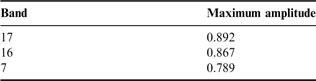
Lastly, the three Bark bands with the highest amplitudes, together with these values, are also stored (see Table 1). The Bark analysis is an auditory modeller that provides perceptually meaningful data, corresponding to the intensity of the first 24 critical bands of hearing. Furthermore, when compared to 512 band FFTs, the analysis itself already provides useful data reduction.

Table 1

Maximum Bark amplitudes for the three most intense bands of an example soundfile.

Each sample library’s complete analysis file, spectrum_DB, is written to disk as text, and is read prior to use in performance.

4.1. Organisation

In addition to the analysis file described in Section 3.2, the fuzzy comparison requires an additional array to be created prior to performance: samples_by_bands is created at this time, in which pointers to spectrum_DB indices are sorted into the 24 Bark energy bands. For example, if a sample’s Bark bands are (2 5 7), the spectrum_DB index is entered into samples_by_bands at all three locations. This allows access to all samples that have high energy in a specific band.

4.2. Real-time implementation

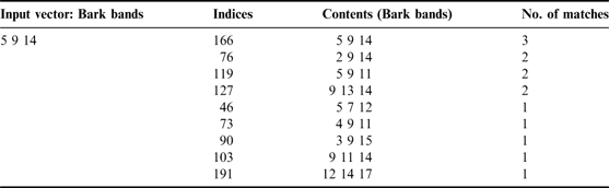
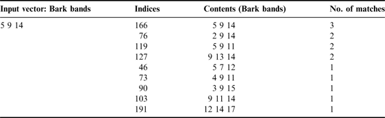
In performance, an input vector representing three Bark bands is passed to samples_by_bands, which returns an array of all sample indices whose three highest bands contain any of those values. The array’s contents are then compared to the input vector, and the number of direct matches is used to sort the list (see Table 2). Those samples that are most similar, according to their highest three Bark bands, are at the top of the sorted array, while all entries will contain at least one match.

Table 2

An example input vector and results returned by samples_by_bands, sorted by number of direct matches between the contents and the input vector.

This algorithm only works if the input vector matches the analyses within the database, which is not always the case. Furthermore, only exact matches are returned, rather than similar matches. For this reason, fuzzy comparisons are made, by including adjacent bands in the search.

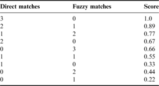
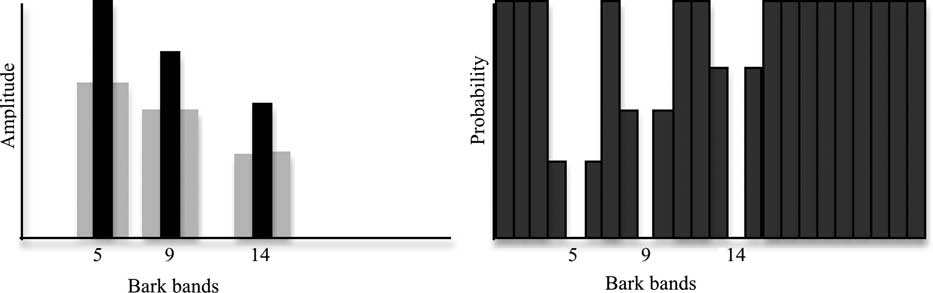
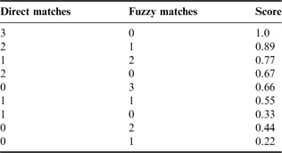
A ‘fuzzy list’ is created around the input vector by including adjacent bands: for example, given an input vector of (5 9 14), the following fuzzy list is generated: (4 6 8 10 13 15). The number of direct matches between the input vector and the returned bands are summed, matches to the fuzzy list are summed and scaled by 0.66 (a hand-tuned value that created the ordering in Table 3), and the two values summed. The result is scaled to between 0 and 1 to create a closeness rating (see Table 3).

Table 3

Closeness ratings based upon matching bands between results returned by samples_by_bands, and the input vector.

4.3. Real-time applications

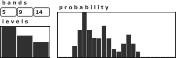
One possible application for this method is the selection of samples that are similar (or dissimilar) to timbres performed live. Incoming timbres can be analysed to derive the three most intense Bark bands, and this input vector used to derive a set of similar samples. Similarly, the user can set the probabilities by hand, by selecting three bands and their relative levels (see figure 1).

Figure 1

Defining a spectral band from which to choose a sample by setting three bands and their relative energies to determine probabilities.

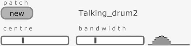
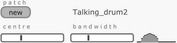
A faster method used in the generative rhythm software (Eigenfeldt Reference Eigenfeldt2009) would be to select an approximate spectral bandwidth, from which the software can use a Gaussian probability distribution to generate a random input vector (see figure 2). This would tend to select samples whose Bark bands are close together, which is useful when discrete spectral bands are desirable.

Figure 2

Using only a centre frequency and bandwidth to define a spectral band from which to choose a sample.

4.4. Search heuristics

Since the search space can contain several hundred items, even when limited by using the pre-sorted samples_by_bandsarray, it was found that evaluating it in its entirety (using a 16-nearest neighbour implementation) took too long in performance; often several seconds. Therefore, a heuristic algorithm was created to find enough (16) acceptable solutions within an acceptable amount of time (less than 1,500ms).

Incrementing through the search space in order and selecting samples until the desired number is reached would consistently create the same results given the same input vector. In the case of generative software, which is often the case for live laptop music, this is not a desired compositional choice; indeed, different results are desirable given the same input values. Therefore, the sample list is incremented randomly until the desired number of selections are made.

When the randomly incremented search first begins, only ratings of 0.67 and higher are acceptable (see Table 3). After 250 ms, this is enlarged to include scores of 0.66 and above, therefore including samples without any direct matches, but with three fuzzy matches. After 1,000 ms, it is enlarged to include scores of 0.55 and above, including those samples with only one direct match and one fuzzy match. During the search, results are added to the samples list and loaded to be immediately available for performance.

4.5. Dissimilarity

It is often desirable to select samples that are dissimilar to a given input vector. For example, given an input timbre that contains mainly high-frequency energy, it could be useful to choose accompanying timbres that contain mainly low frequencies, as these would constitute a distinctly separate spectrum, and thus avoid timbral masking.

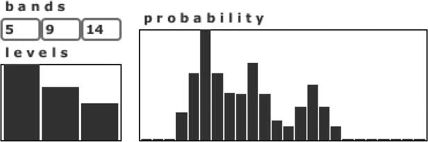
Choosing dissimilar timbres to a given Bark set is simply a matter of creating an inverse probability vector around the three bands (see figure 3a), then choosing three new bands using probabilities from this vector (see figure 3b), and finally searching for timbres with these bands.

Figure 3

(a) An input vector of (5 9 14) and its ‘fuzzy list’ (left). (b) The inverse of this vector, used as a probability distribution for selection of dissimilar timbres (right).

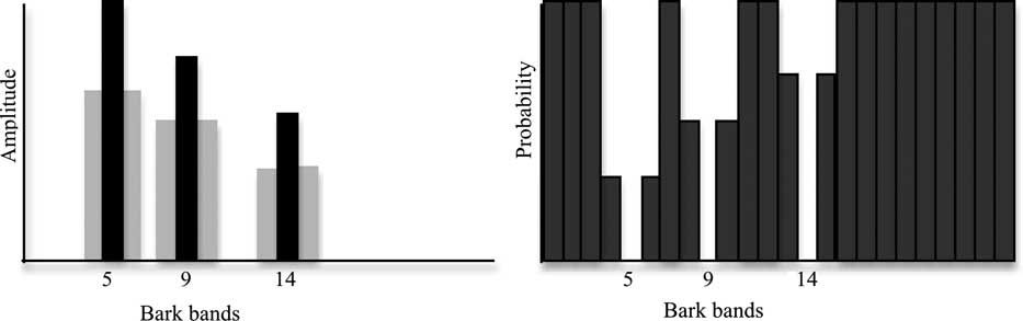
If the dissimilar bands are generated only once prior to selection, the resulting timbres will all be related, since they share the same bands; for example, generating three dissimilar Bark bands by random selection using the probability vector from figure 3b might result in a Bark band vector of (2 12 18). If this single vector were used to select multiple samples from the database, these samples would all share that vector and thus have similar timbres. However, the same inverse probability vector can generate a different set after each sample selection. This would result in each sample being dissimilar to the original, yet with a high probability of dissimilarity within the new sample groups.

5.1. Generation of the self-organising maps

A SOM was implemented in MaxMSP to create a two-dimensional representation of the sample database. SOMs are a type of artificial neural network using a neighborhood function so as to reflect feature proximity in a topologic manner.

For purposes of comparison to Method 1, the input vector consisted of a sample’s 3 highest Bark bands’ numbers, between 0 and 23, scaled to between 0 and 1; however, the input vector can easily be changed to use any feature data, and be of any size (see Section 5.4). The visualisation map was a 25–by-25 Jitter matrix, representing the 625 individual nodes (artificial neurons), with the three weights of each node (one per band) mapped to RBG values. The grid itself is toroidal; that is, opposite edges are connected.

5.1.1. Training

Each node’s weights were initialised to random values between 0 and 1. The number of training iterations (ti) was defined as 10,000 for the sample database of 1,551 items. The initial neighborhood size (ins) was half that of the map: 12 nodes in every direction. The initial learning rate (lr) was set to 1, and decreased at a logarithmic rate at each training iteration (t) using the following function:

Similarly, the neighborhood size (ns) decreased at a logarithmic rate:

At each iteration a training example, chosen randomly from the database, is fed to the network and the Euclidean distance to all weight vectors is computed. The winning vector (the best matching unit, or BMU), is the node with the weight vector most similar to the vector of the input instance.

The weights of the BMU and those nodes in the neighborhood are then adjusted towards the input vector. The differences between their current weight and the input vector are multiplied by the weight scaling function (ws), and then added to the original weights:

Self-organisation initially takes place on the global scale (since the initial neighbourhood is covering the entire map), whereas over time the neighbourhood shrinks to what is eventually a single node and the weights converge to local estimates.

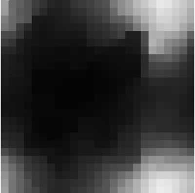
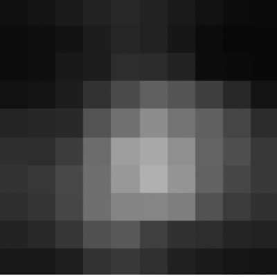
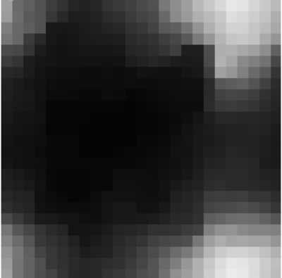
Once training is complete, the SOM will display those samples that are similar to one another in close proximity (see figure 4). Here the shades displayed relate to the input vector (the three most intense Bark bands). Dark colours represent those samples in which all three Bark bands are low; light colours represent those samples in which all three Bark bands are high; those that are closer to one primary colour represent samples whose Bark bands are spread out – in other words, a given Bark band vector of (17 3 5) will be bright red (not displayed in the grayscale image).

Figure 4

An example visualisation of the SOM of the percussion sample library, displayed in grayscale.

5.2. Mapping

Once training is complete, it is possible to directly associate individual nodes and input vectors. The database was incremented in its entirety (one additional epoch), and fed to the SOM. Each BMU was used as the index into an array of matching samples.

For the SOM shown in figure 4, only 52% of the nodes had one or more samples associated with them; however, of those with associations, the mean number of associations was 4.85, with a maximum of 139 sample files per node. This duplication of associations resulted from samples within the database having essentially identical data (e.g. the three most intense Bark bands). While this demonstrates the clustering functionality of the SOM, it is impractical for the user. See Section 5.4 for a more productive use of the SOM.

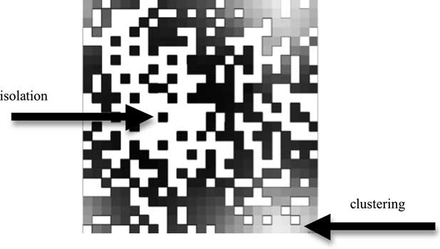
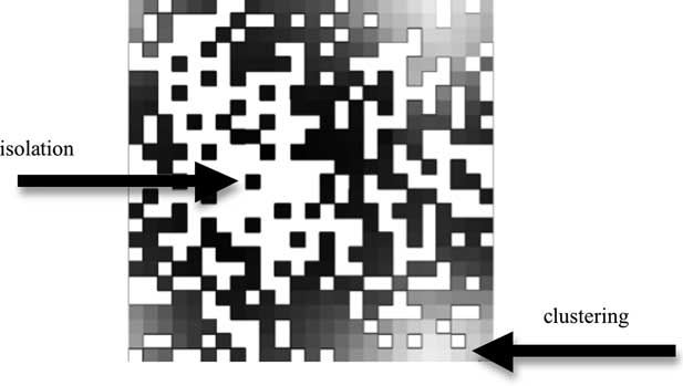
The SOM can also be visualised to show only the direct associations, with non-associated nodes remaining white; thus, this visualisation shows potential clustering of data (see figure 5). Note, for example, the relative isolation of certain nodes, which signifies few similarities within the database to those samples. Compare this to the clusters of light squares at the bottom right (which also wrap around to the top of the map); this signifies a clustering of similar samples within the database. This particular visualisation does not display how many samples are associated with each node; however, implementing the z-axis for this purpose would rectify this.

Figure 5

The associated SOM from figure 4, displaying the unassociated nodes as white. This shows which nodes are isolated, as well as those that are clustered.

5.3. Real-time implementation

An obvious benefit of using a SOM is its ability to visualise similarities within a database. The most practical real-time implementation of a SOM allows the user to click on a visual map, and derive the appropriate association(s) from the database. This is a simple matter of converting the <x,y> mouse selection coordinates in an index into the association array. Using the post-learning associative matrix (figure 4), which clearly displays learnt associations, only items in the database that directly correlate to the visual display will be returned.

5.4. Choice of features to display

As with any SOM, the effectiveness of the visualisation is in the choice of features displayed. It was found that the best features to choose were those that had significant differences within the database.

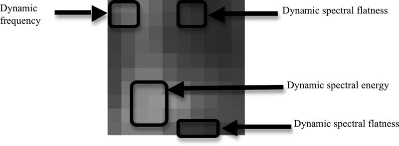
For example, figure 6 displays the soundscape database, using the standard deviation of the sample’s brightness, loudness, and noise over its duration. Squares that display red are associated with samples that have greater dynamic frequency (spectral centroid) change; squares that display green have greater variation in their spectral energy; those squares that display blue have greater dynamic change in their spectral flatness. These areas in the grayscale SOM are highlighted (see figure 6).

Figure 6

SOM visualising the soundscape database, using standard deviation of brightness, loudness and noise after three epochs. Since the database has fewer items, the matrix was reduced to 10 × 10.

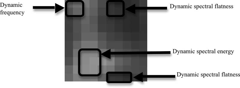
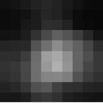
Figure 7 displays the selected GarageBand loop database using mean brightness, standard deviation of brightness and mean frequency. In this case, dark squares contain low frequencies, and have little change in their spectral centroid (i.e. the bass samples), the brightest squares have higher spectral energy, with dynamic spectral change (i.e. percussion samples).

Figure 7

SOM visualising the GarageBand loop database using mean and standard deviation for brightness, and mean frequency.

5.5. Larger feature sets

Since the Bark analysis produces 24 discrete intensity values, it was possible to train the SOM using all 24 values as an input vector. Using the GarageBand loops, after 64 epochs (about 100,000 training iterations), finer delineations between data allowed more associations to be made. In the case of figure 6, while only 46% of the squares had direct sample associations after 1 epoch, over 82% had associations after 64 epochs.

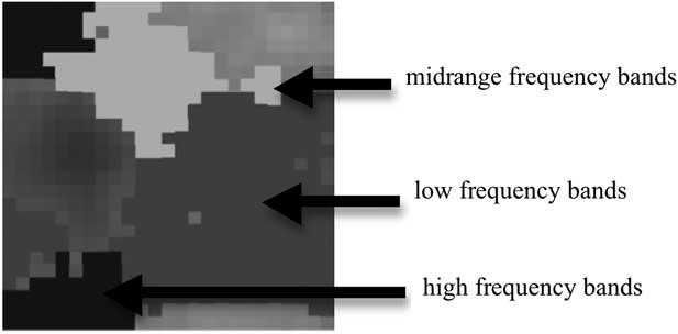
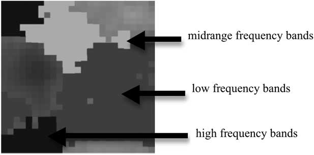
Visualising 24 inputs in two dimensions required mapping the 24 weights of each node to the three RGB values. The averages over eight bands’ intervals were used. As a result, red squares indicate energy primarily in low-frequency bands, green squares indicate energy in the mid-range frequency bands, and blue squares indicate energy in the high-frequency bands (see a simplified grayscale version in figure 8).

Figure 8

SOM visualising 24 Bark bands of GarageBand loops using mean amplitude.

5.6. Real-time applications

It was found that the most effective use of SOMs in performance displayed several visualisations at once, allowing the user to make selections in one or more of the maps and correlate the resulting selections. For example, by using one SOM to display temporal information (such as figure 5), and one to display frequency content, it is possible to select items from the database that are associated with both selections.

Another useful application was to draw paths through the visualised data, to be interpreted over time. For example, using the visualisation in figure 5, a path was drawn from the top left through the bottom middle, which was interpreted over a ten-minute performance. During this time, samples could be automatically selected, beginning with dynamic frequency change and ending with dynamic noisiness.

6.1. Benefits to Method 1

Because the fuzzy logic system uses heuristics, enough acceptable solutions will always be found. In cases where a specific number of solutions are required, this is of great benefit; for example, in the case of Eigenfeldt (Reference Eigenfeldt2009), which utilises a set number of agent-based performers. The method offers a very simple and efficient selection mechanism. The user can choose a type of timbre by specifying dominant spectral energy, either through three bands (as in figure 1), or a frequency centre and bandwidth (as in figure 2), and move towards a similar or dissimilar sound in one click.

6.2. Detriments to Method 1

Although acceptable solutions will always be found, depending upon the input criteria, the level of acceptability can vary greatly. Since this method does not visualise the database, it is possible to define criteria that do not exist within the database. This is especially true if the database is relatively small. While our aim is to investigate real-time sample selection based mainly on timbral similarity, this method reduces it to very basic spectral information. As is often the case, there is a trade-off between user interface simplicity and quality of the control obtained.

6.3. Benefits to Method 2

SOMs visualise the actual database, which can influence the design of the database itself; for example, if not enough high-frequency samples are present, the SOM can display this, and adjustments can be made. Multiple SOMs can be used to display different features, and different features can even be visualised within a single SOM. In fact, SOMs are extremely flexible in their ability to display similarities over any kind of data. Perhaps the greatest benefit of SOMs to real-time performers is no actual calculations – other than conversion of mouse location to database indices – are necessary: all intensive calculations are done prior to performance.

6.4. Detriments to Method 2

This is a very generic method, as opposed to the ad hoc heuristic approach of Method 1. Although SOMs allow easy visualisation, it is not immediately clear what is being visualised; for example, knowing what a red pixel represents, as opposed to a blue, requires an understanding of the analysis itself. Of course, this can be easily addressed by providing the user with the proper documentation, and designing a user interface that balances simplicity and control.

Since SOMs involve time-consuming training, they are not real-time, and therefore cannot display any new data.

Lastly, there is no easy way (at least compared to point and click) of selecting a range of selections or associations. In other words, the SOM (as discussed here) does not display the number of associations behind any square, and thus guaranteeing a certain number of selections (see Section 6.1) is more difficult.