


I. Introduction
The price that financial markets place on sovereign default risk is a core component of the cost of borrowing for governments and shapes how capital moves across countries. The postpandemic rise in public debt and the 2022–2024 monetary tightening have renewed a long-standing question: how do macroeconomic fundamentals enter the price of sovereign risk (e.g., Rogoff (Reference Rogoff2022))? That they enter at all is well established; country-specific fundamentals retain substantial explanatory power even after controlling for global factors and credit ratings (Hilscher and Nosbusch (Reference Hilscher and Nosbusch2010)), and a sovereign country’s fiscal capacity governs how growth shocks pass through to its default risk (Augustin, Sokolovski, Subrahmanyam, and Tomio (Reference Augustin, Sokolovski, Subrahmanyam and Tomio2022)).
What remains less clear is where in the data those fundamentals appear and in what form. Longstaff, Pan, Pedersen, and Singleton (Reference Longstaff, Pan, Pedersen and Singleton2011) find that sovereign credit default swaps (CDS) spreads are driven mainly by global factors. Ang and Longstaff (Reference Ang and Longstaff2013) documents a systemic component common to U.S. and European sovereigns, whereas Augustin (Reference Augustin2018) shows the balance between global and domestic risk shifts with the slope of the CDS term structure. A separate thread reads the time variation in estimated macro-sensitivities as episodes in which spreads detach from fundamentals (Balduzzi, Savona, and Alessi (Reference Balduzzi, Savona and Alessi2023)). These accounts share a modeling choice: each estimates the mapping from fundamentals to spreads within the class of linear models.
We ask whether this linearity assumption, rather than the fundamentals, drives the literature’s conclusion. Theory gives reason to doubt it. Doshi, Ericsson, Jacobs, and Turnbull (Reference Doshi, Ericsson, Jacobs and Turnbull2013) derive a no-arbitrage framework in which the CDS term structure responds nonlinearly to the macroeconomic state, generating threshold effects and regime-contingent loadings that no linear interaction of state variables and maturity can reproduce. We therefore study the shape of the mapping from macroeconomic fundamentals to sovereign CDS premiums: the functional form through which fundamentals price sovereign risk, and in particular whether it is non-monotone, varies across maturities, and shifts with the economic regime. If the mapping has this shape, a linear model misstates both how much fundamentals matter and which fundamentals matter.
Our premise is that sovereign CDS premiums measure the price of default risk, isolating it from the interest-rate and liquidity effects that also move bond yields. The analysis uses a panel of 25 macroeconomic indicators for 25 OECD economies from January 2008 to December 2024, with daily CDS spreads at four maturities as the forecasting target. This is a broader, higher-frequency sample than the panels used in prior CDS studies (see Section III). The panel spans five macroeconomic regimes, from the global financial crisis through the 2022–2024 monetary tightening cycle. We use macro variables at their first-release (“real-time”) value to avoid look-ahead contamination rather than as an identifying treatment; our findings are quantitatively similar when we use the corresponding revised vintages, which we report in Section C of the Supplementary Material.
We compare two broad classes of forecasting models: linear specifications spanning model-averaging, penalized regression, and principal component methods, and nonlinear specifications including non-parametric methods (tree ensembles and support vector regression (SVR)), and a feed-forward neural network (NN). Because out-of-sample
$ {R}^2 $
 in a panel setting is highly sensitive to the benchmark used to evaluate forecasts, we report results against four nested benchmarks that isolate the cross-country, cross-maturity, and within-country-and-maturity components of CDS variation.
The article makes three main contributions. First, we document that the linear class fails to forecast sovereign CDS premiums across both the cross-maturity and cross-country dimensions during the 2022–2024 monetary tightening, whereas tree-based ensembles forecast accurately across both dimensions. Every linear specification delivers a negative yearly
$ {R}^2 $
 in every year when forecasts are evaluated against a benchmark that isolates maturity-level variation. Maturity interactions and principal-component reduction do not change this. Extreme gradient boosting (XGBoost), in contrast, is positive in 15 of 16 years at the 1-month horizon. Against a benchmark that isolates country-level variation, linear performance is initially strong but deteriorates post-2022. Elastic Net’s yearly 1-month cross-country
$ {R}^2 $
 on the Global panel falls from an average of 0.53 over 2011–2021 to 0.31 over 2022–2024, while XGBoost shows no such deterioration. SVR forecasts accurately along both dimensions but by smaller margins, while a NN does so only weakly.
Second, the functional form of XGBoost forecasts is state-dependent in economically interpretable ways. Out-of-sample Shapley values (Shapley (Reference Shapley, Kuhn and Tucker1953), Lundberg, Erion, Chen, DeGrave, Prutkin, Nair, Katz, Himmelfarb, Bansal, and Lee (Reference Lundberg, Erion, Chen, DeGrave, Prutkin, Nair, Katz, Himmelfarb, Bansal and Lee2020)) show that the predictor attribution is not time-invariant: the term-structure slope is the persistently dominant predictor, year-over-year inflation is activated primarily during the 2022–2024 tightening cycle, and consumer confidence is mostly relevant during the Eurozone sovereign debt crisis. Elastic Net, by contrast, reads sovereign credit risk through the debt-to-GDP ratio with an attribution pattern that is nearly time-invariant. Partial dependence plots refine the reading. The response of expected CDS premiums to the term structure is monotone increasing with a regime-dependent slope, and the regime in which the slope flattens most is the monetary tightening cycle—where the inflation channel activates through a threshold-like step. A linear specification that fits a single coefficient per predictor across all regimes cannot capture these state-dependent shapes.
A key concern is whether these shapes are panel-wide regularities or artifacts of country-specific fits. Our third contribution is to show that they hold over the whole panel of countries. A leave-one-country-out (LOO) exercise, in which each sovereign is held out of the training sample in turn, shows that the state-dependent mappings tree ensemble fits transport across countries. Because cross-country variation accounts for roughly 73% of the total log-CDS variance, the LOO MSE primarily measures how well each method extrapolates the cross-country ordering of CDS levels to a country absent from the training set. XGBoost beats Elastic Net in 22 of 25 countries, with a 59% pooled MSE reduction, and the magnitude of the advantage orders by how idiosyncratic the held-out country’s macro fundamentals are: largest for emerging markets, intermediate for the European periphery, and smallest for core OECD economies.
Our findings speak directly to the empirical literature on macroeconomic fundamentals and sovereign CDS spreads. Longstaff et al. (Reference Longstaff, Pan, Pedersen and Singleton2011) attribute variation in sovereign CDSs mainly to global factors; our design also considers country-specific indicators, so our evidence on predictor relevance complements their decomposition rather than testing it. Once nonlinearity is allowed, predictor relevance reorders relative to the linear class: the term-structure slope—the signal Augustin (Reference Augustin2018) identifies as central—is the dominant predictor across regimes even though the linear specifications leave it unused, while the debt and deficit ratios on which those specifications and the broader literature load fall to secondary. Inflation, the short-rate response, and consumer confidence enter only in specific regimes. Finally, what the LASSO of Balduzzi et al. (Reference Balduzzi, Savona and Alessi2023) reads as price variation unrelated to fundamentals is, in our setting, reconciled through the lens of nonlinearity.
Our methodological approach connects to two further strands of literature. Machine-learning methods have been applied extensively to sovereign default classification (e.g., Manasse, Schimmelpfennig, and Roubini (Reference Manasse, Schimmelpfennig and Roubini2003), Fioramanti (Reference Fioramanti2008), Basu and Perrelli (Reference Basu, Perrelli and Xin2019), and Silva, Rego, and Frascaroli (Reference da Silva, Rêgo and Frascaroli2019)) but remain underused for sovereign risk pricing, where Belly, Boeckelmann, Caicedo Graciano, Di Iorio, Istrefi, Siakoulis, and Stalla-Bourdillon (Reference Belly, Boeckelmann, Graciano, Di Iorio, Istrefi, Siakoulis and Stalla-Bourdillon2023) is a notable exception, applying ML to euro-area sovereign bond spreads over the pre-COVID period. We adapt the out-of-sample
$ {R}^2 $
 evaluation framework that Gu, Kelly, and Xiu (Reference Gu, Kelly and Xiu2020) and Bianchi, Büchner, and Tamoni (Reference Bianchi, Büchner and Tamoni2021) apply to equity and bond return prediction to the sovereign CDS setting, and characterize predictor-level functional forms with Shapley-value feature attribution and partial dependence plots. The Shapley decomposition replaces the reduction-in-
$ {R}^2 $
 importance measure used in that literature with a fully allocated attribution of the drivers of expected CDS premiums.
II. A Simple Motivating Framework
A single-name CDS is an over-the-counter credit derivative contract that provides protection against the default of a specific reference entity. The buyer pays a premium, known as the CDS spread, to the seller in exchange for compensation in the event of a default. The premium reflects the perceived risk of default.
To motivate the use of machine learning methods, we build on a standard no-arbitrage argument that equates the discounted cash flows of the CDS buyer and seller. The resulting pricing expression nests the log-linear specifications used in the empirical sovereign-CDS literature as a special case and makes explicit the functional-form assumptions they impose.
Assume that the buyer seeks compensation equal to
$ L=1-R $
 , where
$ R\in \left[0,1\right) $
 is the recovery rate and
$ L $
 represents the expected loss as a fraction of the notional. The seller charges the buyer a continuously paid premium
$ {S}_{j,t}^{\ast } $
 at time
$ t $
 . At time
$ t $
 , the two parties agree on the maturity
$ t+j $
 and the compensation
$ L $
 payable if the reference entity defaults. For simplicity, we assume no counterparty risk, meaning the premium depends solely on the reference entity’s default risk.
Under these conditions, the premium leg of the CDS represents the seller’s cash inflows, discounted to present value:

where
$ {\unicode{x1D540}}_{\left\{\tau >t\right\}} $
 is an indicator of no default before time
$ t $
 ,
$ \tau $
 is the random default time,
$ {\mathrm{\mathcal{F}}}_s={\left\{{\mathbf{x}}_{s-i}\right\}}_{i\ge 0} $
 represents the filtration generated by the state variables, and
$ {r}_s $
 and
$ g\left({\mathbf{x}}_s\right) $
 are the risk-free discount rate and default intensity rate, respectively, at time
$ s $
 . The expression implies that the seller’s cash flows are discounted at a higher rate of
$ {r}_s+g\left({\mathbf{x}}_s\right) $
 , reflecting both the time value of money and default risk.
The default leg of the CDS represents the discounted compensation paid in the event of default before maturity:

Under no-arbitrage conditions (e.g., Augustin and Tédongap (Reference Augustin and Tédongap2016)), the CDS premium is considered “fair” when the present values of the premium and default legs are equal,
$ PL\left({S}_{j,t}^{\ast };t,t+j\right)= DL\left({S}_{j,t}^{\ast };t,t+j\right) $
 . Assuming a constant recovery rate
$ R $
 and a first-order small-spread approximation, this yields an approximate pricing expression for the CDS spread of maturity
$ j $
 :

The dependence of the spread on the state is therefore mediated through the default intensity process
$ g\left({\mathbf{x}}_u\right) $
 . Appendix A provides the explicit derivation and the conditions under which the approximation holds.
We collapse the forward-looking expectation in the pricing expression into a reduced-form function of the state by defining
$ \gamma \left({\mathbf{x}}_{t-1},j\right)\equiv {\unicode{x1D53C}}_t\left[\frac{1}{j}{\int}_t^{t+j}g\left({\mathbf{x}}_u\right)\hskip0.1em du|{\mathbf{x}}_{t-1}\right] $
 , which gives the log spread

where
$ \gamma \left(\cdot, j\right) $
 is a (possibly unknown) function of the state vector
$ {\mathbf{x}}_{t-1} $
 for each maturity
$ j $
 . Equation (3) is the starting point for our empirical exercise: it is deliberately agnostic about the functional form of
$ \gamma $
 , and the predictability of
$ {s}_{j,t} $
 from one-lag conditioning macroeconomic variables
$ {\mathbf{x}}_{t-1} $
 depends on how well a chosen specification for
$ \gamma $
 approximates the true mapping.
The benchmarking approach in the empirical CDS literature assumes a log-linear approximation of equation (3),

which yields the familiar linear predictive regression
$ {s}_{j,t}\propto \boldsymbol{\beta} {(j)}^{\prime }{\mathbf{x}}_{t-1} $
 (e.g., Gourieroux, Monfort, and Polimenis (Reference Gourieroux, Monfort and Polimenis2006)). Under equation (4), term-structure slopes
$ \boldsymbol{\beta} \left({j}_1\right)-\boldsymbol{\beta} \left({j}_2\right) $
 are deterministic functions of
$ j $
 alone, and maturity interactions with the state take a strictly additive form (Balduzzi et al. (Reference Balduzzi, Savona and Alessi2023)). If equation (4) is an adequate approximation, then linear regressions and their penalized variants with maturity dummies exhaust the predictable variation in sovereign spreads.
In contrast, if the default intensity depends on the state non-monotonically and the shape of that dependence varies with maturity, the CDS term structure is itself a nonlinear function of the state. Doshi et al. (Reference Doshi, Ericsson, Jacobs and Turnbull2013) derive this result in a no-arbitrage, discrete-time setting and show that it produces threshold effects and regime-contingent loadings that cannot be spanned by linear interactions between the state variables and maturity dummies. Determining whether cross-maturity nonlinearity is present in the data is one of the tasks in Section IV.
A distinct implication concerns the short-horizon dynamics of the spread at fixed country-maturity
$ \left(i,j\right) $
 . The persistence of log CDS spreads, combined with infrequent macroeconomic releases at a daily frequency, implies that
$ {s}_{j,t} $
 exhibits little predictable variation relative to its own country-maturity trailing mean,
$ {\overline{s}}_{ij} $
 . Any macro-driven specification—linear or nonlinear—is therefore expected to underperform
$ {\overline{s}}_{ij} $
 at short horizons. Section IV documents this and evaluates forecasts against benchmarks that capture cross-country or cross-maturity variation rather than within-country-maturity variation. We interpret the within-country-maturity underperformance as a mechanical consequence of state dynamics and release frequency rather than as evidence against the macro-to-CDS link.
Related evidence for nonlinearity in sovereign spread dynamics is provided by Augustin and Tédongap (Reference Augustin and Tédongap2016), Doshi, Jacobs, and Zurita (Reference Doshi, Jacobs and Zurita2017), and Chernov, Schmid, and Schneider (Reference Chernov, Schmid and Schneider2020), with complementary work on endogenous structural breaks in credit risk (e.g., Galil, Shapir, Amiram, and Ben-Zion (Reference Galil, Shapir, Amiram and Ben-Zion2014), Jeanneret (Reference Jeanneret2015), Blommestein, Eijffinger, and Qian (Reference Blommestein, Eijffinger and Qian2016), and Lahiani, Hammoudeh, and Gupta (Reference Lahiani, Hammoudeh and Gupta2016)) pointing to further sources of nonlinearity in the mapping from macro fundamentals to sovereign credit risk. Building on this foundation, our empirical exercise takes equation (3) as the object to estimate and tests whether the log-linear approximation equation (4) is an adequate representation of
$ \gamma \left(\cdot, j\right) $
 . Evidence of improved out-of-sample prediction accuracy from a nonlinear specification over the linear benchmark implies that the former is a closer approximation to
$ \gamma \left(\cdot, j\right) $
 than the log-linear null.
III. Data and Research Design
We collect daily CDS premiums for 3-, 5-, 7-, and 10-year maturity contracts on a panel of 25 OECD economies spanning developed and emerging markets over January 2008 to December 2024. Sovereign CDS spreads are sourced from Bloomberg. All contracts use the Complete Restructuring (CR) clause and are denominated in U.S. dollars, with the exception of Canada (No Restructuring, XR) and the United States (CR, denominated in euros).Footnote 1 Section B of the Supplementary Material reports the restructuring clause, currency, and earliest available date for each country-maturity pair. The panel includes Austria, Belgium, Canada, Chile, the Czech Republic, Denmark, Estonia, Finland, France, Germany, Hungary, Ireland, Italy, Japan, Korea, Mexico, the Netherlands, Poland, Portugal, the Slovak Republic, Slovenia, Spain, Sweden, the United Kingdom, and the United States.
The 17-year window encompasses the 2008–2009 global financial crisis, the 2010–2012 European sovereign debt crisis, the postcrisis low-rate decade, the 2020 COVID-19 pandemic, and the 2022–2024 monetary tightening cycle in response to post-COVID inflationary pressures, providing substantial variation in the economic environments under which CDS premiums are priced.
Figure 1 presents a snapshot of the sample variation in the 5-year CDS spread over time and across countries. Countries with weaker economic fundamentals, such as Ireland, Italy, Spain, and Portugal, exhibit consistently higher and more volatile premiums, and cross-country dispersion peaked during the European sovereign debt crisis. Despite the severity of the 2020 shock, CDS spreads during the COVID-19 outbreak remained relatively subdued compared to historical crisis periods.
Figure 1 reports the month-year cross-sectional distribution of the daily 5-year CDS premium (Graph A) and the country time series distribution of the 5-year CDS premium (Graph B). The sample period is daily from January 2008 to December 2024.

FIGURE 1 Long description
A two-panel figure displaying C D S premium data in basis points (b p s).
Graph A: Distribution of 5-year C D S over time.
- The x-axis represents years from 2008 to 2024.
- The y-axis represents C D S premium across countries (b p s) ranging from 0 to 1700.
- The data is presented as a series of vertical box plots for each time period.
- A significant spike is visible between 2011 and 2013, where premiums reach their peak near 1400 to 1500 b p s.
- Following 2014, the distribution stabilizes at a lower level, generally remaining below 400 b p s, with minor fluctuations around 2020 and 2023.
Graph B: Distribution of 5-year C D S across countries.
- The y-axis lists 26 countries vertically, starting from United States at the top to Austria at the bottom.
- The x-axis represents C D S premium over time (b p s) from 0 to 1600.
- Horizontal box plots show the spread for each nation.
- Portugal and Hungary show the widest distributions and highest median premiums, with Portugal’s outliers extending beyond 1600 b p s.
- Countries like the United States, United Kingdom, Germany, and France show very narrow distributions concentrated near the 0 to 100 b p s range.
The combination of daily frequency and a broad cross section places our sample at the recent end of the sovereign CDS literature. Studies that extend further back do so at a lower frequency. Longstaff et al. (Reference Longstaff, Pan, Pedersen and Singleton2011) use monthly spreads for 26 countries over 2000–2010, and Augustin (Reference Augustin2018) uses monthly spreads for 44 countries from 2001 to 2012. Broad daily panels appear only after the global financial crisis, once single-name sovereign contracts became liquid across a wide set of reference entities, as in the 38-sovereign daily network of Bostanci and Yilmaz (Reference Bostanci and Yilmaz2020) from 2007 to 2019. The closest design to ours is Balduzzi et al. (Reference Balduzzi, Savona and Alessi2023), who pair daily CDS with real-time macroeconomic data for a small cross section of European sovereigns over 2009–2020. Relative to these later studies, our panel is wider and longer, covering the COVID pandemic and the 2022–2024 tightening cycle.
The panel’s variance structure shapes how forecasting performance should be interpreted. On the pooled 2009–2024 sample of log CDS spreads, cross-country differences account for approximately 73% of total variance, cross-maturity differences for approximately 16%, and within-country-maturity time variation for the remaining 11%.Footnote 2 The dominance of the cross-country component and the small within-country-maturity share motivate the nested-benchmark evaluation design in Section IV, which isolates where, in the variance decomposition, each forecasting method succeeds or fails.
A. Macroeconomic Indicators and Preprocessing
Our predictor set combines macroeconomic indicators from the “Revisions Analysis Dataset—Infra-annual Indicators” of the OECD Main Economic Indicators (MEI) database with sentiment indicators from the OECD Key Short-Term Economic Indicators data set, country-specific economic policy uncertainty indexes developed by Baker, Bloom, and Davis (Reference Baker, Bloom and Davis2016),Footnote 3 and financial variables from Bloomberg. The predictor block covers real-sector indicators, fiscal and inflation measures, financial variables (interest-rate spreads, stock indices, USD exchange rates), and global factors such as the VIX and the global economic activity index of Kilian (Reference Kilian2009), incorporating the correction discussed in Kilian (Reference Kilian2019).
Two small variable choices are worth noting. The OECD Composite Leading Indicator (CLI) was discontinued in the OECD Revisions Database after 2022; we replace it with two sentiment-based indicators from the OECD Key Short-Term Economic Indicators data set, the business confidence indicator (BCI) and the consumer confidence indicator (CCI), both available over the full sample. The EPU index of Baker et al. (Reference Baker, Bloom and Davis2016) is not available for all countries in our panel; we approximate missing values using the EPU series of a neighboring country with close economic and geographical ties (Sweden for Finland, Spain for Portugal, and so on). Table A1 in Appendix B lists each variable together with its source and transformation code, and the average correlation structure is reported in Section B of the Supplementary Material.
We align our predictor transformations with the FRED-MD convention of McCracken and Ng (Reference McCracken and Ng2016) to ensure that the predictor block is stationary by construction. Each indicator is mapped to one of four transformation codes (tcode). Let
$ {x}_t $
 denote the original series and
$ {\tilde{x}}_t $
 the transformed predictor; we use

with
$ p=12 $
 for the monthly series and
$ p=4 $
 for the quarterly series, so that differences and growth rates are measured year-over-year. The variable-by-variable mapping is reported in Table A1 in Appendix B. GDP and its real-activity components enter as year-over-year percentage changes; price and activity indices as year-over-year log differences; unemployment and short-term interest rates as year-over-year first differences; and scale-free ratios, sentiment indicators, and global financial factors in levels.
The stationarity of the target variable—the log CDS spread—is a separate question. Panel unit-root tests (Pesaran (Reference Pesaran2007)) and stationarity tests (Kwiatkowski, Phillips, Schmidt, and Shin (Reference Kwiatkowski, Phillips, Schmidt and Shin1992), Hadri (Reference Hadri2000)) reject their respective nulls for all four CDS maturities at the 5% level or better; the combined pattern points to high persistence of log CDS spreads with slowly drifting levels, consistent with the characterization of sovereign credit spreads in Longstaff et al. (Reference Longstaff, Pan, Pedersen and Singleton2011) and Augustin (Reference Augustin2018). The transformed predictor block is stationary by construction under the FRED-MD transformations. The forecasting results reported in Section IV are unlikely to be affected by spurious correlations. Detailed test results are reported in Section B of the Supplementary Material.
Timing and Frequency Alignment
The target variable is observed daily, while macroeconomic predictors are released monthly or quarterly. We use each macroeconomic variable at its first-release (“real-time”) value rather than at ex post revised values, which aligns the predictor block with the information set available to market participants at each forecast date (following the broader real-time tradition of Croushore and Stark (Reference Croushore and Stark2001), Orphanides (Reference Orphanides2001), Ghysels, Horan, and Moench (Reference Ghysels, Horan and Moench2018)). The daily frequency of the target, aligned to these first-release indicators, is what makes a real-time macroeconomic predictor block of this breadth usable: monthly sovereign-spread studies, with far fewer target observations per estimation window, are typically restricted to more compact, lower-frequency predictor sets. Appendix A provides an example of the original data structure from the OECD MEI database.
Aligning daily CDS observations with lower-frequency predictor releases requires a choice of interpolation. We follow the forward-filling convention used in the yield-curve forecasting literature (Coroneo, Giannone, and Modugno (Reference Coroneo, Giannone and Modugno2016), Caruso and Coroneo (Reference Caruso and Coroneo2023)). This implies that each macroeconomic variable is held constant at its most recent release value until a new release occurs, so that between two consecutive releases, the last observed value is the only predictor realization in any investor’s information set. Figure A2 in Appendix B illustrates the alignment procedure and the release-date assumptions used when the exact release date is not recorded in the source data.
We note that the frequency mismatch in our setting is the reverse of that motivating the MIDAS family (Ghysels, Sinko, and Valkanov (Reference Ghysels, Sinko and Valkanov2007), Ghysels et al. (Reference Ghysels, Horan and Moench2018)), where a lower-frequency target is forecast from higher-frequency predictors. In our setting, the target is higher-frequency than the predictors, so MIDAS lag polynomials do not apply directly. The natural MIDAS analogs—reverse-MIDAS specifications or mixed-frequency state-space models (Foroni, Guérin, and Marcellino (Reference Foroni, Guérin and Marcellino2018))—impose a parametric stochastic model on the high-frequency component of the predictor between macro releases, effectively treating the intra-release period as containing news inferred from interpolation rather than observed.
In contrast, forward-filling treats the intra-release period as containing no new available information, consistent with the literal structure of the data-release process by policymakers. Each forward-filled predictor block is then the common input to all forecasting methods in Section III.B, linear and nonlinear alike, so that differences in out-of-sample performance reflect the mapping from predictors to CDS rather than the handling of the frequency mismatch.
B. Forecasting Methods and Evaluation Protocol
We compare eight linear specifications against five nonlinear specifications in a unified out-of-sample protocol. The linear models implement the log-linear benchmark of equation (4); the three nonlinear families relax it through distinct representational mechanisms—recursive partitioning of the feature space, kernel-based feature expansions, and hierarchical nonlinear transformations.
Every method receives the same set of macroeconomic indicators
$ {\mathbf{x}}_{i,t-1} $
 and four CDS maturity dummies, with the maturity dummies entering as interactions in the linear specifications and as ordinary predictors in the nonlinear specifications. For every method that either shrinks coefficients toward 0 or trains on cross-sectionally demeaned targets, we subtract the cross-country mean at each time and maturity before estimation, and recenter the maturity-specific means at the forecast stage, thereby preventing shrinkage or demeaning from contaminating the maturity-interaction structure.
1. Linear Specifications
Following Balduzzi et al. (Reference Balduzzi, Savona and Alessi2023), we adopt a “level + slope” form that interacts the real-time macroeconomic indicators
$ {\mathbf{x}}_{i,t-1} $
 (plus an intercept) with the CDS maturity
$ j $
 ,

where
$ {m}_j $
 is a dummy variable that takes the value 1 if the contract has a
$ j $
 -year maturity, and 0 otherwise,
$ \mathcal{J}=\left\{\mathrm{3,5,7,10}\right\} $
 , and the 3-year CDS is the reference group. On top of this common form, we consider three strategies for managing the high dimensionality of the predictor block in short rolling windows: coefficient regularization (Ridge, Lasso, Elastic Net; Hsiang (Reference Hsiang1975), Tibshirani (Reference Tibshirani1996), and Zou and Hastie (Reference Zou and Hastie2005)), forecast combination via Complete Subset Regression (CSR; Elliott, Gargano, and Timmermann (Reference Elliott, Gargano and Timmermann2013)) and its equal-weighted special case (EWC; Rapach, Strauss, and Zhou (Reference Rapach, Strauss and Zhou2010)), and latent-factor dimension reduction via Principal Component Regression (PCR; Ludvigson and Ng (Reference Ludvigson and Ng2009), Stock and Watson (Reference Stock, Watson, Clements and Hendry2011), and Kelly and Pruitt (Reference Kelly and Pruitt2013)) and Partial Least Squares (PLS). Implementation details are in Section A of the Supplementary Material. For robustness, we also estimate “level-only” variants of each linear specification that omit the maturity-interaction terms in equation (6), and report the corresponding results in Section C of the Supplementary Material.
2. Tree-Based Methods
The first nonlinear family is based on recursive partitioning of the feature space (e.g., Breiman, Friedman, Stone, and Olshen (Reference Breiman, Friedman, Stone and Olshen1984), Döpke, Fritsche, and Pierdzioch (Reference Döpke, Fritsche and Pierdzioch2017), and Medeiros, Vasconcelos, Veiga, and Zilberman (Reference Medeiros, Vasconcelos, Veiga and Zilberman2021)). At each node, the feature space is split on a predictor
$ {x}_{i,t-1,p} $
 (the
$ p $
 -th component of the state vector
$ {\mathbf{x}}_{i,t-1} $
 ) and a cutoff value
$ c $
 , chosen jointly to minimize the within-region sum of squared errors of the target
$ {s}_{ij,t} $
 ,

with
$ {I}_{<}=\left\{\left(i,j,t\right)|{x}_{i,t-1,p}\le c\right\} $
 ,
$ {I}_{>}=\left\{\left(i,j,t\right)|{x}_{i,t-1,p}>c\right\} $
 , and leaf predictions equal to the mean target value in each region. We consider three variants that control a fully grown tree’s tendency to overfit. A pruned regression tree penalizes leaf count directly. A random forest (Breiman (Reference Breiman2001)) averages over an ensemble of trees trained on bootstrap samples, with a random subset of predictors evaluated at each split. XGBoost (Chen and Guestrin (Reference Chen and Guestrin2016)) trains a sequence of trees in which each new tree is fit to the gradient of a regularized loss function, yielding an additive ensemble:

with
$ \mathrm{\mathcal{F}} $
 the space of regression trees. Implementation details for all these tree-based methods are in Section A of the Supplementary Material.
3. Kernel-Based Methods
We estimate an
$ \varepsilon $
 -SVR model with a radial basis function (RBF) kernel (e.g., Cortes and Vapnik (Reference Cortes and Vapnik1995), Drucker, Burges, Kaufman, Smola, and Vapnik (Reference Drucker, Burges, Kaufman, Smola, Vapnik, Mozer, Jordan and Petsche1996)). SVR minimizes a regularized
$ \varepsilon $
 -insensitive loss, trading residuals smaller than
$ \varepsilon $
 against the Euclidean norm of the feature-space coefficients; the RBF kernel
$ {K}_{\kappa}\left(u,v\right)=\exp \left(-\kappa \parallel u-v{\parallel}^2\right) $
 —where
$ \kappa $
 is the kernel bandwidth—implicitly maps predictors into an infinite-dimensional feature space, yielding a globally smooth predictor. While recursive partitioning approximates nonlinearities via threshold splits, SVR approximates them via RBF expansions centered at support vectors. Implementation details are in Section A of the Supplementary Material.
4. Neural Networks
We consider a feedforward NN following the architecture of Gu et al. (Reference Gu, Kelly and Xiu2020), adapted to our demeaned panel-data setting. The network has four fully connected hidden layers with 32, 16, 8, and 4 units, ReLU activations, batch normalization after each hidden layer, and dropout regularization (0.50 in the first three hidden layers, 0.25 in the last). The model is trained with the Adam optimizer, early stopping on the validation loss, and a ReduceLROnPlateau schedule. As for SVR, training uses cross-sectionally demeaned inputs and targets, and forecasts are recentered at the maturity mean. NNs approximate nonlinearities through compositions of affine transformations and nonlinear activations, a third distinct representational mechanism relative to the tree-based and kernel-based families. Full implementation details are documented in Section A of the Supplementary Material.
5. Training, Validation, and Testing Protocol
We evaluate the predictive performance of each model on an expanding panel of nonoverlapping testing months. At each testing month
$ t $
 and for a given forecasting horizon
$ h\in \left\{1\mathrm{M},3\mathrm{M},6\mathrm{M},12\mathrm{M}\right\} $
 , we apply the following step-by-step procedure.
-
i) Sample partition. Define the training window as the 12 months preceding $ t $
 ,
$ \left[t-12,t-1\right] $
, pooling all 25 countries and four maturities, and the testing window as
$ \left[t,t+h\right] $
. No observation dated
$ t $
or later is used at any step before step (v).
-
ii) Hyperparameter search by time-series cross-validation. Within the training window, we implement a fivefold forward-chaining cross-validation, illustrated for the 1-month testing horizon in Section A of the Supplementary Material. Each fold uses the earliest portion of the training window to fit model parameters and the subsequent block to compute validation loss; fold boundaries do not overlap, preserving chronological order. For each candidate hyperparameter configuration on a prespecified grid, we record the average validation loss across the five folds.
-
iii) Hyperparameter freezing. We select the configuration $ {\hat{\boldsymbol{\vartheta}}}_t^{\star } $
that minimizes the average validation loss. From this point on,
$ {\hat{\boldsymbol{\vartheta}}}_t^{\star } $
is fixed for the entire testing window
$ \left[t,t+h\right] $
: it is not retuned, updated, or perturbed based on test-period realizations. -
iv) Final fit. Holding $ {\hat{\boldsymbol{\vartheta}}}_t^{\star } $
fixed, we refit the model on the full 12-month training window
$ \left[t-12,t-1\right] $
to obtain the final parameter estimates
$ {\hat{\boldsymbol{\psi}}}_t $
. The validation observations’ role is limited to hyperparameter selection in step (iii); they do not contribute to
$ {\hat{\boldsymbol{\psi}}}_t $
through any channel other than their presence in the common training window. -
v) Out-of-sample forecasting. Using $ \left({\hat{\boldsymbol{\vartheta}}}_t^{\star },{\hat{\boldsymbol{\psi}}}_t\right) $
, we generate daily out-of-sample forecasts for the testing window
$ \left[t,t+h\right] $
. No model object, hyperparameter, or fit weight is updated during the testing window. -
vi) Rolling advance. We advance $ t $
by 1 month and repeat steps (i)–(v). Each model is therefore retrained monthly on a rolling basis.


This protocol has three features that address concerns about the statistical reliability of machine-learning out-of-sample results. First, the data partition at each
$ t $
 satisfies a strict temporal ordering: training precedes validation, which precedes test, with no observations from the testing window entering the training or validation steps. Second, test-period observations do not feed back into hyperparameter choices or parameter estimates, since
$ {\hat{\boldsymbol{\vartheta}}}_t^{\star } $
 and
$ {\hat{\boldsymbol{\psi}}}_t $
 are frozen at the end of step (iv). Third, the rolling structure of step (vi) ensures that any parameter drift between testing months reflects only new training data, not repeated peeks at the test block. A time-series split preserves the temporal dependencies inherent in macroeconomic variables and sovereign CDS premiums, avoiding the look-ahead bias that would arise from random shuffling. The rolling-window estimation also accommodates the structural shifts and regime changes highlighted in Section II and documented empirically in Section IV (see also Pesaran and Timmermann (Reference Pesaran and Timmermann2007), Clark and McCracken (Reference Clark and McCracken2009), and Pesaran and Pick (Reference Pesaran and Pick2011)).
IV. On the Predictability of CDS Premiums
We compare the forecasting performance of each model based on the out-of-sample
$ {R}_{t, oos}^2 $
 , as defined in Campbell and Thompson (Reference Campbell and Thompson2008):

where
$ {s}_{ij,\tau } $
 is the observed log CDS premium for country
$ i $
 , maturity
$ j $
 , at day
$ \tau =1,\dots, \mathcal{T} $
 within the monthly testing period
$ t=1,\dots, T $
 , and
$ {\hat{s}}_{ij,\tau } $
 refers to the log premium predicted by a given model. Equation (9) compares a given forecast with a “no-predictability” benchmark from a prevailing sample mean
$ \overline{s} $
 , estimated over the training period.
We consider four distinct settings for the naive forecast
$ \overline{s} $
 , each absorbing a different source of variation in the panel:

The four benchmarks are ordered along a natural hierarchy of predictive severity, and they admit a direct interpretation in terms of the dimension of CDS variation each benchmark leaves in the denominator of the
$ {R}^2 $
 . Against
$ {\overline{s}}_{\cdot j} $
 , which does not vary across countries, a positive
$ {R}^2 $
 reflects the model’s ability to generate country-specific predictions that improve on a maturity-level constant; the
$ {R}^2 $
 against this benchmark measures cross-country predictability. Against
$ {\overline{s}}_{i\cdot } $
 , which does not vary across maturities, a positive
$ {R}^2 $
 reflects the ability to generate maturity-specific predictions that improve on a country-level constant; the
$ {R}^2 $
 measures cross-maturity predictability. The grand mean
$ {\overline{s}}_{\cdot \cdot } $
 is the least demanding benchmark, since it absorbs neither dimension;
$ {\overline{s}}_{ij} $
 is the most demanding, since it absorbs both and leaves only within-country-maturity time variation in the denominator.
The severity of each benchmark reflects the panel’s variance structure.Footnote
4 As discussed in Section III, the panel’s variance is dominated by the cross-country component, with the cross-maturity and within-country-maturity components accounting for progressively smaller shares. This asymmetry is reflected in the
$ {R}^2 $
 levels each benchmark delivers: the more of the total variance the benchmark absorbs, the smaller the denominator of the
$ {R}^2 $
 , and the harder it is for any model to achieve a positive score.
All forecasting methods in Section IV.B are fitted once per rolling month on the full 25-country panel, and subgroup results are obtained by restricting the summations in equation (9) to the countries in each subgroup rather than retraining on a country subset. This design choice keeps the training sample size—25 countries and four maturities over a 12-month window—constant across subgroups, so that subgroup comparisons are apples-to-apples in their training input. The three subgroups are the South-West Eurozone Periphery (SWEAP: Spain, Portugal, Italy, Ireland), OECD non-EU, and EU ex-SWEAP; the results for SWEAP and OECD non-EU are reported in the main text alongside the Global panel, whereas the results for EU ex-SWEAP are reported in Section C of the Supplementary Material.
A. Time-Varying Predictability
We begin with the yearly out-of-sample
$ {R}^2 $
 , which we compute as the average of
$ {R}_{t, oos}^2 $
 within each calendar year. Figure 2 reports the yearly
$ {R}^2 $
 on the Global panel, 2010–2024, across two benchmarks (rows) and two forecasting horizons (columns).Footnote
5 The heatmap colors each yearly cell by its
$ {R}^2 $
 value, with blue shading for positive values, red shading for negative values, and white at 0; cells with
$ \mid {R}^2\mid \ge 0.7 $
 are annotated.
Figure 2 reports the annual average of
$ {R}_{t, oos}^2 $
 on the Global panel of 25 countries. Graphs A and B use the benchmark
$ {\overline{s}}_{\cdot j} $
 (log CDS averaged across countries); Graphs C and D use
$ {\overline{s}}_{i\cdot } $
 (averaged across maturities). Columns: 1-month (Graphs A and C) and 3-month (Graphs B and D) testing horizons. Cells are colored by
$ {R}^2 $
 using a diverging scale centered at 0; values with
$ \mid {R}^2\mid \ge 0.7 $
 are annotated.

FIGURE 2 Long description
A four-panel grid of heat maps showing yearly out-of-sample R super 2 values.
Common Structure:
* Y-axis: Eight models listed as X G B, R F, S V R, N N, E W C, C S R, P C R, and E Net.
* X-axis: Years from 2010 to 2024.
* Color Scale: A diverging vertical bar on the right ranging from 1.00 (dark blue) through 0.00 (white) to -1.00 (dark red).
Panel Breakdown:
* Top-Left (Graph A, Cross-Country, 1-Month): Predominantly blue, indicating positive R super 2. X G B shows the highest consistency with values between 0.71 and 0.91. R F and S V R also show strong performance. E W C is a white horizontal band at zero.
* Top-Right (Graph B, Cross-Country, 3-Month): Similar to Graph A but with slightly lighter blue shades. X G B remains the top performer with values ranging from 0.74 to 0.87.
* Bottom-Left (Graph C, Cross-Maturity, 1-Month): Shows a sharp divide. The top four models (X G B to N N) are mostly blue or light orange. The bottom four models (E W C to E Net) are dark red, with E W C showing extreme negative values like -4.05 and -3.29 in the early 2010s.
* Bottom-Right (Graph D, Cross-Maturity, 3-Month): Similar to Graph C but with more intense red across the bottom half. E W C continues to show the most significant negative performance, with values such as -4.15 and -3.25.
The results pin down where linear methods succeed, where they fail, and where nonlinear methods extend the region of positive out-of-sample performance. Against the cross-country benchmark
$ {\overline{s}}_{\cdot j} $
 (Graphs A and B), Elastic Net and CSR are positive in nearly every year of the 2010–2024 sample, averaging around 0.43 at the 1-month horizon and 0.34 at the 3-month horizon; PCR, restricted to five principal components, is weaker by roughly 0.20 but preserves the sign pattern. The equal-weighted combination (EWC), which strips the linear class of its coefficient structure, collapses to essentially 0 at both horizons, confirming that the cross-country signal is not an aggregation artifact. This suggests that macro fundamentals—debt-to-GDP, growth, unemployment, financing conditions—carry sufficient cross-country signal for linear specifications with regularization to recover positive predictability. Tree-based ensembles improve on this benchmark (XGBoost averages 0.81 at 1-month, Random Forest 0.76), so nonlinearity contributes in the cross-country dimension as well.
The picture changes for the cross-maturity benchmark
$ {\overline{s}}_{i\cdot } $
 . Linear methods fail in every cell of Graphs C and D, with negative
$ {R}^2 $
 in every year at both horizons. The antecedent is Doshi et al. (Reference Doshi, Ericsson, Jacobs and Turnbull2013): in a no-arbitrage CDS pricing model, slope and curvature of the term structure depend on state variables through threshold effects and regime-contingent slope changes that linear maturity interactions cannot span. Tree-based ensembles close the cross-maturity gap most completely. XGBoost is positive against
$ {\overline{s}}_{i\cdot } $
 at 1-month in every year of the 2010–2024 sample, averaging
$ +0.49 $
 . Random Forest is positive in 12 of 15 years (mean
$ +0.31 $
 ), with 2010, 2011, and 2022 being the three negative cells. SVR is positive in 12 of 15 years from 2013 onward, with systematically smaller magnitudes (mean
$ +0.23 $
 ). The feedforward network is negative in 9 of 15 years. The cleavage lies between tree-based ensembles, which capture interactions between maturity and macro state without researcher-specified structure, and the kernel and neural alternatives.
Linear cross-country predictability also weakens under regime change. Elastic Net’s 1-month
$ {R}_{oos}^2 $
 against
$ {\overline{s}}_{\cdot j} $
 drops from an average of 0.54 over 2011–2021 to 0.32 over 2022–2024. At a 3-month horizon, Elastic Net’s 2022 cell is 0.04, compared to 0.68 for XGBoost. Section C of the Supplementary Material shows that the pattern sharpens at 6-month and 12-month horizons. Nonlinear methods retain the signal (XGBoost’s 1 M mean moves from 0.85 in 2011–2021 to 0.82 in 2022–2024), so the weakening is not about fundamentals becoming uninformative but about linear coefficients failing to transport when the mapping from fundamentals to CDS is state-dependent. This suggests that the “disconnect” suggested by prior literature (e.g., Balduzzi et al. (Reference Balduzzi, Savona and Alessi2023)) is more a statement about the rigidity of linear specifications than about the information content of macro fundamentals.
Figure 3 reports the SWEAP subpanel, representing countries sharing a monetary regime and a common crisis history. Elastic Net averages 0.57 at 1-month and 0.53 at 3-month against
$ {\overline{s}}_{\cdot j} $
 , against 0.47 and 0.40 in Global and 0.41 and 0.30 in OECD non-EU. The same specification nonetheless shows negative cross-maturity in most years (Elastic Net mean:
$ -0.52 $
 at 1-month). The Doshi et al. (Reference Doshi, Ericsson, Jacobs and Turnbull2013) term-structure nonlinearity is a within-country property of the pricing mapping and is therefore not attenuated by restricting to a more homogeneous subpanel. The linear cross-maturity failure holds in the group where the linear cross-country fit is strongest.
Figure 3 reports the annual average of
$ {R}_{t, oos}^2 $
 for the SWEAP country subgroup (Spain, Portugal, Italy, and Ireland). Rows: cross-country predictability against
$ {\overline{s}}_{\cdot j} $
 (Graphs A and B) and cross-maturity predictability against
$ {\overline{s}}_{i\cdot } $
 (Graphs C and D). Columns: 1-month (Graphs A and C) and 3-month (Graphs B and D) testing horizons. Models and formatting follow Figure 2.

FIGURE 3 Long description
A multi-panel set of four heatmaps labeled Graph A through Graph D. A shared vertical color bar on the right indicates Yearly Out-of-Sample R super 2 values, ranging from dark red at negative 1.00 to dark blue at positive 1.00, with white at 0.00. The Y-axis for all graphs lists models: X G B, R F, S V R, N N, E W C, C S R, P C R, and E Net. The X-axis spans from 2010 to 2024.
* Graph A (Top-Left): Cross-Country Predictability at a 1-month horizon. The top four models (X G B, R F, S V R, N N) show dominant blue shading with R super 2 values frequently between 0.70 and 0.94. P C R shows significant negative performance in 2021 (negative 0.96) and 2023 (negative 0.93).
* Graph B (Top-Right): Cross-Country Predictability at a 3-month horizon. Similar to Graph A but with slightly lower positive values, mostly ranging from 0.70 to 0.91 in the top four rows. P C R shows a deep red cell at negative 0.99 in 2021.
* Graph C (Bottom-Left): Cross-Maturity Predictability at a 1-month horizon. The bottom four models (E W C, C S R, P C R, E Net) are dominated by dark red, indicating strong negative R super 2 values. E W C shows extreme negative values such as negative 14.50 in 2012. The top four models show lighter blue and white cells.
* Graph D (Bottom-Right): Cross-Maturity Predictability at a 3-month horizon. Follows the trend of Graph C with intense red shading in the bottom half. E W C reaches a low of negative 15.16 in 2012. S V R shows a sharp drop to negative 3.97 in 2012.
In the OECD non-EU subpanel, the institutional setting is the opposite: no shared monetary regime, no common crisis history, and country-level fundamentals ranging from AAA-rated borrowers to investment-grade emerging markets. Figure 4 shows that nonlinear methods nevertheless deliver positive cross-maturity
$ {R}^2 $
 . XGBoost averages
$ +0.39 $
 over a 1-month horizon (14 of 15 years positive), and Random Forest
$ +0.21 $
 (10 of 15), while every linear specification has a negative mean. The nonlinear cross-maturity advantage, therefore, reflects the functional-form gap at the sovereign level rather than the institutional commonality visible in SWEAP.
Figure 4 reports the annual average of
$ {R}_{t, oos}^2 $
 for the OECD non-EU country subgroup. Rows: cross-country predictability against
$ {\overline{s}}_{\cdot j} $
 (Graphs A and B) and cross-maturity predictability against
$ {\overline{s}}_{i\cdot } $
 (Graphs C and D). Columns: 1-month (Graphs A and C) and 3-month (Graphs B and D) testing horizons. Models and formatting follow Figure 2.

FIGURE 4 Long description
A four-panel grid of heatmaps. Each panel shares a common X-axis representing years from 2010 to 2024 and a Y-axis listing eight models: X G B, R F, S V R, N N, E W C, C S R, P C R, and E Net.
* Graph A (Top-Left): Cross-Country Predictability at a 1-month horizon. The top four models (X G B, R F, S V R, N N) show high performance indicated by dark blue cells, with specific R-squared values like 0.92 and 0.91 visible around 2016. The bottom four models show lighter blue or white cells, indicating lower positive performance.
* Graph B (Top-Right): Cross-Country Predictability at a 3-month horizon. Similar to Graph A but with generally lighter blue shades, indicating a slight decrease in predictive power as the horizon increases.
* Graph C (Bottom-Left): Cross-Maturity Predictability at a 1-month horizon. This panel shows a stark contrast. The top models maintain some blue (positive) values, but the bottom models, particularly E W C, are dominated by dark red cells with negative values such as -3.88 and -3.42.
* Graph D (Bottom-Right): Cross-Maturity Predictability at a 3-month horizon. This panel shows the most significant negative performance, with deep red across the bottom five models. E W C shows values as low as -3.65 and -3.43.
A vertical color bar on the right side serves as the legend for all panels. It ranges from -1.00 (dark red) to 0.00 (white) to 1.00 (dark blue), labeled Yearly Out-of-Sample R super 2.
B. Four-Benchmark Aggregate Results
We now turn to full-sample averages of the yearly
$ {R}^2 $
 , organized by benchmark and horizon. Table 1 reports the average
$ {\overline{R}}_{oos}^2 $
 on the Global panel for the eight level + slope linear specifications and five nonlinear specifications, against each of the four benchmarks, at each horizon.Footnote
6 Table 1 is organized so that scanning a single model column from top to bottom traces the
$ {R}^2 $
 decomposition as the benchmark becomes more demanding; scanning a single row compares models at a fixed benchmark and horizon.

TABLE 1 Long description
The table is organized into five forecasting horizon blocks: 1-month, 3-month, 6-month, 9-month, and 12-month. Each block contains four benchmark rows: s-bar dot dot (grand mean), s-bar dot j (cross-country), s-bar i dot (cross-maturity), and s-bar ij train (within-cell training mean).
Columns are divided into two main model classes:
1. Level plus Slope Linear Models: O L S, E W C, C S R, Lasso, Ridge, E N, P C R, and P L S.
2. Nonlinear Models: S V R, R T, R F, X G B, and N N.
Key data trends:
* For the 1-month horizon under the grand mean benchmark, X G B (Nonlinear) achieves the highest value at 0.83, while E N (Linear) leads its class at 0.52.
* As the forecasting horizon increases to 12-months, performance generally decreases. For the grand mean benchmark at 12-months, X G B remains the best nonlinear model at 0.61, and C S R is the best linear model at 0.23.
* Negative values are prevalent in the more severe benchmarks (s-bar i dot and s-bar ij train), particularly for linear models like O L S and E W C, which reach values as low as minus 11.14 and minus 10.25 respectively.
* Across almost all horizons and benchmarks, the X G B model in the nonlinear category and either the E N or C S R models in the linear category are highlighted in bold as the best-performing specifications.
The decomposition reading follows the panel’s variance structure. Moving from
$ {\overline{s}}_{\cdot \cdot } $
 to
$ {\overline{s}}_{\cdot j} $
 removes the approximately 16% of total variance attributable to between-maturity differences from the denominator, which modestly lowers every
$ {R}^2 $
 . Elastic Net at 1-month drops from 0.52 to 0.45, XGBoost from 0.83 to 0.81. Moving from
$ {\overline{s}}_{\cdot \cdot } $
 to
$ {\overline{s}}_{i\cdot } $
 removes approximately 73% of the variance attributable to between-country differences, which is a much larger shift: Elastic Net at a 1-month horizon falls to
$ -0.76 $
 , XGBoost to
$ +0.44 $
 . Linear specifications lose nearly all of their
$ {R}^2 $
 in this step; tree-based nonlinear specifications retain a substantial portion of it. The magnitude of the
$ {R}^2 $
 drop between the two middle benchmarks, therefore, suggests that linear specifications’ out-of-sample performance is concentrated in variance that country fixed effects would absorb in-sample, whereas tree-based ensembles generate predictions in the dimension that fixed effects cannot.
The bottom row of each horizon block reports the
$ {R}^2 $
 against
$ {\overline{s}}_{ij} $
 , the 12-month rolling country-maturity training mean. Every model is negative against this benchmark at every horizon; XGBoost is the least negative (
$ -0.64 $
 at the 1-month horizon,
$ -2.77 $
 at the 12-month horizon), and the model ordering is preserved (XGBoost
$ > $
 RF
$ > $
 SVR
$ > $
 linear). This is not evidence against the macro-to-CDS link. Daily log CDS spreads are near-persistent (see Section B of the Supplementary Material), so a trailing country-maturity mean is close to a random-walk forecast, consistent with the characterization of sovereign credit spreads in Longstaff et al. (Reference Longstaff, Pan, Pedersen and Singleton2011) and Augustin (Reference Augustin2018). The difficulty of beating the
$ {\overline{s}}_{ij} $
 benchmark suggests that the productive macroeconomic signal lies more in the cross-country and cross-maturity dimensions than in the time-series dimension (Duffee (Reference Duffee2002)).
Reading within horizon blocks, the results are consistent with the yearly evidence in Section IV.A whereby linear methods capture cross-country but not cross-maturity predictability, and nonlinear methods extend the region of positive
$ {R}^2 $
 into the cross-maturity dimension and cross-country during crisis regimes. Reading across horizon blocks, the
$ {R}^2 $
 degrades as the horizon extends, but the relative ordering of model classes—linear versus nonlinear, and within nonlinear, XGBoost
$ \approx $
 RF ahead of SVR ahead of NN—is preserved. At the 12-month horizon, Elastic Net’s cross-country
$ {R}^2 $
 is indistinguishable from 0.
Across country groups (Section C of the Supplementary Material), the pattern is preserved without qualitative change. Linear methods capture cross-country variation but fail to capture cross-maturity variation in the OECD non-EU, EU ex-SWEAP, and SWEAP panels; nonlinear methods—XGBoost in particular—deliver positive cross-maturity
$ {R}^2 $
 in every subgroup at short horizons. The magnitudes differ: SWEAP countries show higher raw
$ {R}^2 $
 against the grand-mean benchmark at short horizons, reflecting the larger cross-country spread introduced by peripheral Eurozone sovereigns, but the within-group decomposition (the fall from
$ {\overline{s}}_{\cdot j} $
 to
$ {\overline{s}}_{i\cdot } $
 and the sign pattern it produces) is invariant.
C. Testing Predictive Accuracy
This section reports three pieces of evidence on whether the differences in out-of-sample performance documented in Table 1 and Figure 2 are statistically distinguishable. First, we report pairwise tests of predictive accuracy following Qu, Timmermann, and Zhu (Reference Qu, Timmermann and Zhu2023), a modified Diebold–Mariano procedure robust to panel dependence that delivers the raw significance of each model-versus-model comparison. Second, we report the Hansen, Lunde, and Nason (Reference Hansen, Lunde and Nason2011) Model Confidence Set at 75% and 90% confidence levels, which identifies the set of models that cannot be rejected as the best performer given the data. Third, we report Romano and Wolf (Reference Romano and Wolf2005), (Reference Romano and Wolf2016) step-down-adjusted
$ p $
 -values for the pairwise comparisons, controlling the family-wise error rate across the grid of tested hypotheses; this addresses the data-mining concern that the raw Diebold–Mariano
$ p $
 -values ignore the multiplicity of comparisons.
Panels A and B of Table 2 report the first and third tests for XGBoost against each of the 12 rivals, at the 1-month testing horizon. Technical details and the Model Confidence Set output are in Appendix A.

TABLE 2 Long description
The table is divided into two main sections: Panel A for D M z-statistics and Panel B for R W adjusted p-values. Both panels evaluate four regions: Global, O E C D / E U, E U / S W E A P, and S W E A P.
Twelve rival models are listed in the first column: O L S, E W C, C S R, Lasso, Ridge, E N, P C R, P L S, S V R, R T, R F, and N N.
Key data points include:
* O L S: Panel A values range from minus 10.73 to minus 5.32. Panel B p-values range from 0.004 to 0.165.
* E W C: Panel A values range from minus 40.14 to minus 10.28. Panel B p-values range from 0.000 to 0.124.
* C S R: Panel A values range from minus 22.95 to minus 10.20. Panel B p-values range from 0.000 to 0.098.
* Lasso: Panel A values range from minus 20.15 to minus 6.85. Panel B p-values range from 0.000 to 0.124.
* Ridge: Panel A values range from minus 19.09 to minus 6.40. Panel B p-values range from 0.000 to 0.124.
* E N: Panel A values range from minus 21.19 to minus 7.95. Panel B p-values range from 0.000 to 0.124.
* P C R: Panel A values range from minus 12.76 to minus 8.69. Panel B p-values range from 0.003 to 0.050.
* P L S: Panel A values range from minus 9.53 to minus 4.86. Panel B p-values range from 0.005 to 0.167.
* S V R: Panel A values range from minus 7.54 to 3.88. Panel B p-values range from 0.005 to 0.167.
* R T: Panel A values range from 4.45 to 7.81. Panel B p-values range from 0.005 to 0.167.
* R F: Panel A values range from 4.83 to 11.52. Panel B p-values range from 0.003 to 0.167.
* N N: Panel A values range from 7.24 to 9.81. Panel B p-values range from 0.005 to 0.124.
The final row, number of rejections at 10 percent, shows 12 out of 12 for all columns except for Panel B S W E A P, which shows 2 out of 12.
Under the unadjusted test, every XGBoost-versus-rival
$ z $
 -statistic is large and negative, indicating lower mean squared error for XGBoost; importantly, every comparison is significant at the 1% level in every group (
$ \mid z\mid \ge 3.86 $
 ). The Romano–Wolf adjustment is more demanding: in the Global, OECD non-EU, and EU ex-SWEAP panels, XGBoost’s advantage survives familywise error control against all 12 rivals at
$ \alpha =0.10 $
 (maximum adjusted
$ p $
 -value = 0.005 in Global and 0.011 in OECD non-EU, where the marginal rival is SVR in each case). In the SWEAP subgroup, only 2 of 12 comparisons survive at
$ \alpha =0.10 $
 (PCR at
$ p=0.050 $
 , CSR at
$ p=0.098 $
 ). The remaining models, both linear and nonlinear, are indistinguishable from XGBoost under FWER control. The SWEAP pattern reflects the narrower cross section (5 sovereigns vs. 25 in the Global panel) and the correspondingly wider posterior on the loss-differential distribution, while XGBoost retains the lowest mean squared error in every cell, as shown in Section C of the Supplementary Material.
The Model Confidence Set delivers a stronger verdict (see Table A2): at both confidence levels and across all country groups over the 1-month horizon, the MCS contains only XGBoost. That is, no rival model can be retained at the 90% confidence level as statistically indistinguishable from the best forecaster. Put differently, every non-XGBoost specification is rejected from the set of equivalent-best models.
V. Dissecting the Expected CDS Premiums
Section IV documents a sharp split between the linear and nonlinear forecaster classes. Linear methods can capture a great deal of cross-country variation in sovereign CDS premiums but fail to predict cross-maturity variation at any horizon, while tree-based ensembles—XGBoost in particular—deliver positive out-of-sample
$ {R}^2 $
 against both benchmarks at short horizons. This section opens the XGBoost forecaster to identify the predictors that carry this performance, trace the functional shapes they induce, and test whether those mappings are panel-wide regularities or country-specific fits. The comparison is drawn throughout against the best-performing linear specification, the “level + slope” Elastic Net.
We treat the exercise as descriptive. Shapley values are properties of a given prediction, not of the data-generating process; the XGBoost–Elastic Net contrast therefore identifies which dimensions of the predictor space each functional form reaches, not the structural determinants of sovereign default risk. In that sense, the attribution evidence is the mechanism behind the
$ {R}^2 $
 ordering in Section IV, not a claim about the equilibrium CDS premiums.
A. Forecasting Performance Attribution
We measure predictor importance with the Shapley value (Shapley (Reference Shapley, Kuhn and Tucker1953)), which represents the unique additive and monotone allocation of a model’s forecast to its inputs. Additivity means that the predictor contributions sum to the forecast minus a model-specific baseline, so attribution is fully allocated with no residual hidden in an intercept. Monotonicity means that if predictor
$ i $
 raises the forecast by at least as much under one model as under another on every subset, then its Shapley value is at least as large under the first model. The two properties serve complementary roles in our setting. Additivity yields fully allocated attribution within each forecaster, and monotonicity ensures that the attributions are comparable across models fitted to the same inputs.
Formally, let
$ D=\left\{1,\dots, d\right\} $
 index the predictors and
$ v:\mathcal{P}(D)\to \mathrm{\mathbb{R}} $
 be a value function that returns a model’s forecast as a function of which predictors are “present.” The Shapley value of predictor
$ i $
 is

where the weight
$ \mid S\mid !\left(|D|-|S|-1\right)!/\mid D\mid ! $
 is the probability of forming coalition
$ S $
 in a random permutation of the
$ d $
 predictors.Footnote
7 Equation (10) satisfies
$ {\sum}_{i\in D}{\phi}_i(v)=v(D)-v\left(0/\right) $
 , so Shapley values decompose the forecast-minus-baseline into predictor-specific contributions.
A two-predictor example makes additivity concrete. For a forecaster of the term-structure slope (Term) and the debt-to-GDP ratio (Debt/GDP) with
$ v\left(0/\right)=0.01 $
 ,
$ v\left(\left\{\mathrm{Term}\right\}\right)=0.04 $
 ,
$ v\left(\left\{\mathrm{Debt}/\mathrm{GDP}\right\}\right)=0.03 $
 , and
$ v\left(\left\{\mathrm{Term},\mathrm{Debt}/\mathrm{GDP}\right\}\right)=0.05 $
 , equation (10) gives
$ {\phi}_{\mathrm{Term}}=0.025 $
 and
$ {\phi}_{\mathrm{Debt}/\mathrm{GDP}}=0.015 $
 .Footnote
8 The two sum to
$ 0.04=v\left(\left\{\mathrm{Term},\mathrm{Debt}/\mathrm{GDP}\right\}\right)-v\left(0/\right) $
 , and Term receives the larger attribution because its marginal forecast increase is larger whether it is added first or second.
In the empirical implementation, the value function is the model’s out-of-sample forecast with the predictors in
$ S $
 set at their explicand values and the predictors in
$ \overline{S}=D\backslash S $
 integrated over baseline observations drawn from the testing distribution:

where
$ {x}^e $
 is the explicand (the observation being explained),
$ E $
 is the set of baseline observations,Footnote
9 and
$ f\left({x}_S^e,{x}_{\overline{S}}^b\right) $
 denotes the forecast when the predictors in
$ S $
 take the explicand values and those in
$ \overline{S} $
 take the baseline values.Footnote
10
For XGBoost, equation (11) is computed with the TreeSHAP algorithm of Lundberg et al. (Reference Lundberg, Erion, Chen, DeGrave, Prutkin, Nair, Katz, Himmelfarb, Bansal and Lee2020), which exploits the tree structure to return all
$ {\phi}_i $
 simultaneously in time linear in the number of leaves.Footnote
11 For Elastic Net, equation (11) admits the closed form
$ {\phi}_i\left(f,{x}^e\right)={\beta}_i\left({x}_i^e-{\mu}_i\right) $
 , where
$ {\beta}_i $
 is the penalized coefficient on predictor
$ i $
 and
$ {\mu}_i={\left|E\right|}^{-1}{\sum}_{x^b\in E}{x}_i^b $
 is the baseline mean.Footnote
12 Linear attribution is therefore the deviation of the explicand from the baseline mean, scaled by a single penalized coefficient—fixed across countries, across regimes, and across maturities.
In both cases, the forecaster
$ f $
 at each month is the recursive 1-month-ahead estimate used to produce the out-of-sample
$ {R}^2 $
 reported in Section IV. The explicand
$ {x}^e $
 is the corresponding testing observation, and the baseline set
$ E $
 is the set of testing observations, so both the evaluation point and the distribution over which
$ \overline{S} $
 -predictors are integrated lie outside the training window.
B. Time-Varying and Cross-Sectional Attribution
Figure 5 reports the time-varying mean absolute Shapley values for XGBoost (Graph A) and the “level + slope” Elastic Net (Graph B), averaged across countries in the Global panel.Footnote 13 The out-of-sample window spans February 2009 through November 2024, covering the GFC aftermath, the Eurozone sovereign debt crisis, the decade of accommodative policy, the COVID-19 shock, and the 2022–2024 monetary tightening cycle.
Figure 5 displays the out-of-sample mean absolute Shapley values from XGBoost (Graph A) and the “level + slope” Elastic Net (Graph B), averaged across countries in the Global panel at each 1-month testing period. The color scale is sequential (darker indicates higher importance). Rows correspond to the predictors described in Section III.A. The out-of-sample period is February 2009 through November 2024.

FIGURE 5 Long description
A two-panel heat map display.
Panel A, titled XGBoost, shows Mean Absolute S H A P Value on a scale from 0.000 (white) to 0.200 (black). The Y-axis lists 20 macroeconomic variables including C P I, I I P, I R D, G D P, E G S, E G S forward slash G D P, G C E, G F C, I G S, I G S forward slash G D P, P C E, B O P, H U R, I N T, S P, B C I, C C I, Term Spread, F X, Debt forward slash G D P, and E P U. The X-axis spans from 2009 to 2024. In this panel, Term Spread and C C I show the highest sustained importance (darkest shading) across the entire period, particularly between 2011 and 2023. C P I shows a significant spike in importance starting around 2021.
Panel B, titled Elastic Net, uses a different scale for Mean Absolute S H A P Value from 0.0 to 4.0. It shares the same Y-axis variables and X-axis timeline. The importance distribution is more sparse compared to Panel A. The most prominent features are high-importance bands for B C I and C C I between 2010 and 2022, and a very dark, concentrated band for Debt forward slash G D P between 2011 and 2019. G F C shows a localized peak of importance around 2016.
We organize the discussion around three features that together characterize the attribution-level footprint of the cross-maturity
$ {R}^2 $
 failure in Section IV, namely which predictors XGBoost uses and in which regimes, which predictors Elastic Net uses and how its use differs, and how the contrast holds across the cross section of countries.Footnote
14
XGBoost uses the term-structure slope (Term Spread) persistently and inflation-related predictors conditionally. Graph A of Figure 5 shows a dominant Term Spread band across most of the 2011–2024 window; this is the only predictor that carries nontrivial attribution in every regime of the sample. The CCI is activated during the Eurozone sovereign debt crisis (2011–2014) and flares again during the COVID period (2020–2021). The year-over-year change in consumer prices (CPI) and the first difference of the short-term interest rate (INT) are essentially dormant through 2020 and then activate sharply in 2021–2024, together giving the monetary tightening cycle its distinct signature.
Fiscal ratios (Debt/GDP, EGS/GDP, IGS/GDP), the business sentiment indicator (BCI), and country-specific risk proxies (EPU, FX, equity prices) carry secondary or near-zero attribution throughout. The same three-predictor core—Term Spread, CCI, and the tightening-cycle CPI/INT pair—appears in each of the three country subgroups (Figures A3–A5 in Appendix B); the Term Spread band is sharpest in SWEAP and the tightening-cycle CPI/INT activation sharpest in OECD non-EU, but the set of active predictors and their timing are stable across groups.
Elastic Net uses debt and sentiment, not the term-structure slope or inflation. Graph B of Figure 5 is dominated by a persistent Debt/GDP band from 2011 through the mid-2020s, with CCI and BCI as secondary bands of similar structure. The three predictors that carry XGBoost’s attribution most distinctively—Term Spread, CPI, INT—are essentially white in the heatmap throughout Graph B. The tightening-cycle activation visible in Graph A is not present in Graph B; the Eurozone-crisis CCI flare is present but at a much smaller amplitude; Term Spread is unused at any point in the sample.
Expected CDS premiums from Elastic Net are therefore not a muted version of XGBoost’s but depend on a different attribution pattern entirely. The attribution asymmetry is a consequence of functional form.Footnote 15 The linear specification does not adapt its predictor use across regimes, and the predictors it does use are disjoint from those XGBoost relies on. The same ranking holds in the three country subgroups, as shown in Appendix B.
The asymmetry holds country by country. Figure 6 reports the time-averaged attribution separately for each country. For XGBoost (Graph A), Term Spread is the leading or near-leading predictor for essentially every country in the panel, with secondary concentrations on CCI (sharpest in SWEAP and the EU ex-SWEAP periphery) and on Debt/GDP (concentrated on Italy, Hungary, and Mexico). For Elastic Net (Graph B), Debt/GDP dominates, with the largest loadings falling on countries whose debt-to-GDP ratios deviate most from the panel mean—Japan, Korea, Mexico, Hungary, Italy, and the Slovak Republic. The Japan case is the cleanest illustration of the linear mechanism: sovereign CDS premiums on Japan are among the lowest in the sample, yet Elastic Net attributes the largest Debt/GDP-driven component to Japan because the closed form
$ {\phi}_i={\beta}_i\left({x}_i^e-{\mu}_i\right) $
 rewards deviation from the panel mean rather than spread level. The three predictors XGBoost uses most actively—Term Spread, CPI, INT—are white across every country in Graph B. The attribution asymmetry documented in Figure 5 is therefore not an artifact of cross-country averaging; it is a predictor-level property that manifests consistently across all 25 countries in the panel.
Figure 6 displays the mean absolute Shapley values from XGBoost (Graph A) and the “level + slope” Elastic Net (Graph B), with each cell reporting a predictor’s monthly out-of-sample Shapley values averaged across the testing period for the indicated country. Columns are grouped by country group (SWEAP; EU ex-SWEAP; OECD non-EU) and ordered alphabetically within group; rows correspond to the predictors described in Section III.A. The out-of-sample period is February 2009 through November 2024.

FIGURE 6 Long description
Two side-by-side heatmaps, labeled Graph A. X G B o o s t and Graph B. Elastic Net.
Both graphs share a common Y-axis with 20 economic predictors including C P I, I I P, I R D, G D P, E G S, E G S all over G D P, G C E, G F C, I G S, I G S all over G D P, P C E, B O P, H U R, I N T, S P, B C I, C C I, Term Spread, F X, Debt all over G D P, and E P U.
The X-axis lists 24 countries grouped by region.
1. S W E A P: Ireland, Italy, Portugal, Spain.
2. E U ex-S W E A P: Austria, Belgium, Estonia, Finland, France, Germany, Netherlands, Slovak Republic, Slovenia.
3. O E C D non-E U: Canada, Chile, Denmark, Hungary, Japan, Korea, Mexico, Poland, Sweden, United Kingdom, United States.
Graph A (X G B o o s t) uses a grayscale scale from 0.00 to 0.16. It shows high feature attribution (darker cells) consistently across almost all countries for Term Spread and C C I. Specific high-impact cells include C P I for Germany and E G S all over G D P for Hungary and the United States.
Graph B (Elastic Net) uses a grayscale scale from 0.0 to 2.5. The attribution is more sparse compared to Graph A. The highest values are concentrated in the Debt all over G D P row, particularly for Italy, Slovenia, Chile, Mexico, and Poland. C C I also shows significant attribution across most countries, while Term Spread shows moderate attribution compared to its dominance in the X G B o o s t model.
C. Pricing of Macroeconomic Risks
The Shapley evidence in Section V.B shows which predictors XGBoost uses and in which regimes, but not the functional shape of the mapping. Partial dependence plots (Friedman (Reference Friedman2001)) recover that shape. We report PDPs for the six predictors with the largest XGBoost attribution in Figure 5: the term-structure slope (Spread), year-over-year log change in consumer prices (CPI), year-over-year first difference of the short-term interest rate (INT), CCI, debt-to-GDP ratio (Debt/GDP), and BCI.
The partial dependence function of a forecaster
$ \hat{f} $
 with respect to a predictor
$ {x}_S\in \mathrm{\mathbb{R}} $
 is

where
$ {x}_C $
 are the remaining predictors and the expectation is over the testing-period distribution of
$ {x}_C $
 . Shapley values measure predictor
$ i $
 ’s contribution to a single forecast; PDPs measure the conditional mean forecast as a function of
$ i $
 alone.Footnote
16
The linear specification in Section V.B constrains each predictor’s slope to be constant across the training window. If CDS pricing is stable across regimes, the regime curves in Figure 7 should be parallel shifts; if not, they should differ in slope or shape. The results show that they differ in slope or shape, with the largest divergences occurring during the 2022–2024 tightening cycle.
Figure 7 Regime-averaged partial dependence functions from XGBoost for Spread (Graph A), CPI (Graph B), INT (Graph C), CCI (Graph D), Debt/GDP (Graph E), and BCI (Graph F). Regime windows: Eurozone crisis (2011-04 to 2013-03), low-rate period (2016-04 to 2018-03), COVID-19 (2019-05 to 2021-04), tightening cycle (2022-07 to 2024-06). Horizontal axes are demeaned relative to the cross-sectional mean.

FIGURE 7 Long description
A multi-panel set of six line graphs labeled Graph A through Graph F. Each graph plots Average Prediction (log C D S) on the y-axis against a specific economic variable on the x-axis. Four distinct lines represent different time regimes: Eurozone Crisis (blue dashed), Low-Rate Period (green dotted), C O V I D-19 Shock (red dash-dot), and Tightening Cycle (purple solid).
* Graph A. Term Spread: The x-axis ranges from minus 3 to 4. Most regimes show a sharp upward trend starting at 0, while the Tightening Cycle line remains relatively flat after a sharp drop between minus 1 and 0.
* Graph B. C P I (Y o Y change): The x-axis ranges from minus 4 to 6. The Tightening Cycle shows a steep, continuous positive slope, while other regimes show more moderate increases or plateaus after 1.
* Graph C. Short-Term Rate (Y o Y change): The x-axis ranges from minus 0.2 to 0.3. The Tightening Cycle shows a significant upward step-function trend between 0.1 and 0.2, while the Eurozone Crisis line trends downward.
* Graph D. C C I: The x-axis ranges from minus 20 to 50. The Eurozone Crisis line shows a deep trough between minus 10 and 0, stabilizing at a lower level than other regimes which remain relatively flat near 0.
* Graph E. Debt all over G D P: The x-axis ranges from minus 40 to 60. All regimes generally show a positive correlation, with the Eurozone Crisis and Low-Rate lines showing the steepest step-like increases as debt levels rise.
* Graph F. B C I: The x-axis ranges from minus 10 to 30. The Tightening Cycle shows a unique deep V-shaped trough centered around 5, while the C O V I D-19 Shock line shows a sharp increase after 10.
XGBoost’s response to the term spread (Graph A) is monotone increasing in the Eurozone crisis, low-rate, and COVID regimes, with ranges of approximately 1.3, 0.85, and 0.75 log CDS points, respectively. The monetary tightening-cycle curve lies near
$ +0.29 $
 over most of the spread range and is no longer monotonic. Similarly, CCI (Graph D) shows a monotone-decreasing Eurozone-crisis curve: the model assigns lower predicted spreads to countries with higher-than-average consumer confidence.
The economic reading of the term spread and consumer confidence is coupled with CPI and INT (Graphs B and C) and suggests that during 2022–2024, a flatter curve reflected the short-rate response to inflation rather than to deterioration in growth. Both inflation and short-term interest rates primarily affect expected CDS premiums in the tightening cycle. Thus, XGBoost treats inflation above the cross-sectional mean and the short-rate response to it as separate channels.
XGBoost’s response to Debt/GDP (Graph E) is approximately monotone increasing across three regimes, with mild nonmonotonicity around the cross-country mean, and flatter in tightening regimes. The linear component is what Elastic Net captures (see Graph B in Figure 5); XGBoost’s secondary attribution picks up the nonmonotone corrections. Graph F shows BCI as nearly flat in the pre-tightening regimes and a threshold drop from
$ +0.04 $
 to
$ -0.11 $
 log points during tightening. Elastic Net captures the pre-tightening linearity; XGBoost adds the tightening threshold.
Overall, Figure 7 describes one mechanism. XGBoost fits a different mapping in each regime, and each predictor embodies regime dependence that a linear model cannot capture. Term spread breaks in slope and level during tightening; CPI and INT switch from inert to threshold-active; CCI is monotone during the Eurozone crisis and flat elsewhere; and Debt/GDP and BCI each decompose into a linear component, which Elastic Net captures, plus regime-specific nonlinear corrections that only the tree ensemble reaches.
D. Cross-Country Extrapolation
Sections V.B and V.C establish that XGBoost learns sovereign CDS spreads via state-dependent mappings that the linear class cannot capture. They do not establish where those mappings come from. Two readings are consistent with the attribution and partial-dependence evidence. The mappings might be country-specific—that is, what XGBoost fits when it sees Italy’s macro history and Italy’s CDS history jointly—in which case the nonlinear advantage documented in Section IV reflects country-by-country overfitting that is opaque to a coefficient-based estimator. Or the mappings might be panel-wide—regularities in how macro fundamentals price sovereign risk that hold in common across the sample—in which case the nonlinear advantage reflects a structural feature of sovereign pricing that the tree ensemble learns from cross-country variation.
To distinguish the two readings, we conduct a LOO exercise. For each country
$ i $
 , we train every model on the remaining 24 countries and forecast country
$ i $
 ’s daily log CDS spreads from its macroeconomic fundamentals. The MSE is computed over country
$ i $
 ’s four maturities and the full out-of-sample window. Because cross-country variation accounts for roughly 73% of total panel variance (Section III), the LOO MSE measures how well each forecaster’s predictions for a held-out country preserve the cross-country ordering of CDS levels implied by the training set. Linear methods extrapolate using coefficient combinations fit to the other 24 countries; tree ensembles extrapolate using a partition of the feature space that depends on where predictor values lie in the joint distribution. The LOO exercise is thus an indirect test of which form of extrapolation transports.
Table 3 reports the results. Panel A shows that XGBoost has the lowest mean MSE across all models, at 0.45 compared to 1.11 for Elastic Net, with a median country-level ratio (calculated as
$ {\mathrm{MSE}}_{\mathrm{model}}/{\mathrm{MSE}}_{\mathrm{ElasticNet}}-1 $
 ) equal to
$ -0.53 $
 , and wins in 22 of 25 countries. The advantage is not specific to the Elastic Net benchmark. XGBoost has a lower mean MSE than every linear specification, including PLS, which has the best median MSE and the most country wins in the linear class.

TABLE 3 Long description
Panel A, titled Cross-Country Extrapolation by Method, lists models in two blocks.
Linear level plus slope block:
* O L S: Mean M S E 0.87, Median 0.77, Wins 13.
* E W C: Mean M S E 0.80, Median 0.80, Wins 11.
* C S R: Mean M S E 0.80, Median 0.76, Wins 11.
* Lasso: Mean M S E 1.10, Median 0.79, Wins 12.
* Ridge: Mean M S E 1.11, Median 0.77, Wins 13.
* Elastic Net: Mean M S E 1.11, Median 0.76, Wins dash.
* P C R: Mean M S E 0.84, Median 0.61, Wins 14.
* P L S: Mean M S E 0.98, Median 0.52, Wins 21.
Nonlinear block:
* S V R: Mean M S E 0.57, Median 0.37, Wins 20.
* R T: Mean M S E 0.59, Median 0.50, Wins 20.
* R F: Mean M S E 0.57, Median 0.52, Wins 20.
* XGBoost: Mean M S E 0.45, Median 0.39, Wins 22.
* N N: Mean M S E 0.64, Median 0.56, Wins 20.
Panel B, titled XGBoost Versus Elastic Net by Country Group, compares Mean M S E:
* O E C D non-E U (12 countries): XGBoost 0.58, Elastic Net 1.55.
* E U ex-S W E A P (9 countries): XGBoost 0.34, Elastic Net 0.65.
* S W E A P (4 countries): XGBoost 0.33, Elastic Net 0.83.
* All (25 countries): XGBoost 0.45, Elastic Net 1.11.
The gap between mean and median MSE for the linear methods indicates that their poor aggregate performance is driven by a handful of countries whose macro fundamentals lie in the tails of the panel distribution, where coefficient-based extrapolation fails most severely.
Among nonlinear methods, XGBoost is the strongest. Its median country-level ratio against Elastic Net (
$ -0.53 $
 ) exceeds those of SVR (
$ -0.39 $
 ), the regression tree (
$ -0.31 $
 ), the random forest (
$ -0.25 $
 ), and the NN (
$ -0.16 $
 ). The cleavage between gradient-boosted trees and other nonlinear methods, identified in Section IV at the within-panel cross-maturity benchmark, reappears here at the cross-country extrapolation benchmark.
Panel B reports the XGBoost-to-Elastic Net mean MSE ratio for the three country subgroups of Section IV. The XGBoost advantage is largest for OECD non-EU (
$ -0.63 $
 ), intermediate for SWEAP (
$ -0.60 $
 ), and smallest for EU ex-SWEAP (
$ -0.48 $
 ). The OECD non-EU group contains most of the emerging-market sovereigns in the sample, which is consistent with the extrapolation reading; the relatively smaller advantage for EU ex-SWEAP reflects these countries’ macro fundamentals being closer to the panel-typical case.
Overall, the cross-country extrapolation evidence in Table 3 supports a panel-wide reading of the mechanism. Tree-based partitioning fits state-dependent shapes in Section V.C and transports those shapes to held-out countries at a rate that orders by how close each country’s macro fundamentals are to the panel average. This is the cross-country complement to the cross-maturity result in Section IV: XGBoost’s advantage persists after removing country-specific training data because the shapes it fits are panel regularities rather than country-specific fits.
VI. Conclusion
This article studies the mechanism by which macroeconomic fundamentals map onto expected sovereign CDS premiums. Evaluating 13 specifications against four nested benchmarks on a panel of 25 OECD economies over 2008–2024, we find that linear methods recover the cross-country ordering of spreads but fail to predict their cross-maturity variation in every year and at every horizon. Tree-based ensembles predict the maturity structure that the linear class misses and retain their cross-country accuracy throughout the 2022–2024 monetary policy tightening cycle, while linear performance degrades.
The two classes of models, that is, linear versus nonlinear, rely on different predictors. Ensemble learning loads on the term-structure slope, consumer confidence, and inflation through regime-dependent mappings. Elastic Net loads on the debt-to-GDP ratio with near-constant attribution. A LOO exercise confirms that these mappings are panel-wide regularities rather than country-specific fits.
The evidence suggests that macroeconomic fundamentals contain more predictive information about sovereign credit risk than the linear class can extract. The “disconnect” between fundamentals and sovereign spreads documented in earlier work is, in this reading, a statement about the rigidity of the linear specification rather than about the information content of macro fundamentals.
Appendix
This appendix provides auxiliary theoretical results (Section A), data documentation and descriptive statistics (Section B), and additional empirical results (Section C). Implementation details for all forecasting methods are collected in the Supplementary Material.
A. Auxiliary Theoretical Results
This section provides the explicit steps connecting the no-arbitrage condition
$ PL\left({S}_{j,t}^{\ast };t,t+j\right)= DL\left({S}_{j,t}^{\ast };t,t+j\right) $
 in Section II to the pricing expression that precedes equation (3)). Our derivation follows the standard reduced-form setting of Duffie (Reference Duffie1999), Schönbucher (Reference Schönbucher2003), and the exposition in Augustin and Tédongap (Reference Augustin and Tédongap2016).
We define the premium and default legs of a CDS contract with maturity
$ j $
 as


where
$ L=1-R $
 is the loss-given-default, and all other notation follows Section II. Since the CDS premium
$ {S}_{j,t}^{\ast } $
 is fixed at contract inception and does not depend on the integration variable
$ u $
 , we can factor it out of (A1):

Equating (A3) and (A2) and dividing through by the no-default indicator
$ {\unicode{x1D540}}_{\left\{\tau >t\right\}} $
 (which is unity conditional on
$ {\mathrm{\mathcal{F}}}_t $
 prior to default) yields

where we use the shorthand
$ {\unicode{x1D53C}}_t\left[\cdot \right]=\unicode{x1D53C}\left[\cdot |{\mathrm{\mathcal{F}}}_t\right] $
 and make the dependence of the fair premium on the contract maturity
$ j $
 explicit through the subscript. Equation (A4) is a valuation formula under reduced-form pricing with deterministic recovery and no counterparty risk. The CDS spread for maturity
$ j $
 equals the loss given default multiplied by the ratio of expected discounted intensities to expected discount factors, integrated over the contract life.
The ratio in equation (A4) does not admit a closed-form expression without additional structure on the joint dynamics of
$ \left({r}_s,g\left({\mathbf{x}}_s\right)\right) $
 . A standard simplification in the empirical CDS literature exploits the fact that sovereign CDS spreads in our sample are typically small: average 5-year spreads for the 25 countries over 2008–2024 lie below 150 basis points outside crisis episodes, and even during the European sovereign debt crisis remain below 5% for most of the panel. For
$ g\left({\mathbf{x}}_u\right)j $
 small, a first-order Taylor expansion of the exponential
$ {e}^{-{\int}_t^ug\left({\mathbf{x}}_s\right) ds} $
 around unity gives

and the joint discount factor factorizes to first order as
$ {e}^{-{\int}_t^u\left({r}_s+g\left({\mathbf{x}}_s\right)\right) ds}\approx {e}^{-{\int}_t^u{r}_s ds}\cdot \left(1-{\int}_t^ug\left({\mathbf{x}}_s\right) ds\right) $
 . Under this approximation, both integrands in equation (A4) are dominated by the pure risk-free discount factor, and the ratio simplifies. Taking the risk-free rate as approximately constant over the maturity window gives

which is the expression invoked before equation (3) in Section II. The Fubini step in the second equality uses the interchangeability of integration and expectation, which is valid under standard regularity conditions on
$ g\left({\mathbf{x}}_u\right) $
 (see, e.g., Duffie (Reference Duffie1999)).
Taking logs of equation (A5),

Equation (A6) still depends on the entire intensity path over
$ \left[t,t+j\right] $
 . Because the instantaneous intensity
$ g\left({\mathbf{x}}_u\right) $
 is a function of the contemporaneous state, and because the state vector is adapted to
$ {\mathrm{\mathcal{F}}}_t $
 through its predictable component, we summarize the joint dependence on the current state and the maturity in a single functional form, writing
$ {\mathrm{log}}_{\unicode{x1D53C}}\left[\frac{1}{j}\int g\left({\mathbf{x}}_u\right) du\right]=\log \gamma \left({\mathbf{x}}_{t-1},j\right) $
 , which yields equation (3) in Section II. This is where our empirical framework departs from the classical empirical CDS literature. Rather than imposing a log-linear specification on
$ \log \gamma \left({\mathbf{x}}_{t-1},j\right) $
 , we treat it as a flexible function of the state and maturity and estimate it non-parametrically.
Two observations about the small-spread approximation are worth stating explicitly. First, the approximation is tightest when spreads are small and worst when they are large. The approximation, therefore, is likely to attenuate the degree of nonlinearity in our pricing framework relative to a fully nonlinear reduced-form implementation; that is, if anything, the log-linear benchmark in equation (4) understates the nonlinearity the data would reveal under exact pricing. Second, the approximation does not affect the subsequent nonparametric treatment. Equation (3) and the agnostic specification
$ {s}_{j,t}\propto f\left({\mathbf{x}}_{t-1},j\right) $
 are stated in terms of the unknown function
$ \gamma \left(\cdot, j\right) $
 , which equation (A6) derives from the underlying intensity process. Any further discrepancy between the first-order approximation and the exact expression is absorbed into the error between
$ f $
 and the true data-generating process that our empirical exercise estimates.
B. Data Description and Descriptives
This appendix describes the real-time macroeconomic data set used in the main empirical analysis. Section B.1 illustrates the real-time release structure of the OECD Main Economic Indicators (MEI) data. Section B.2 sets out the release date and forward-filling conventions used to align the daily CDS target with the lower-frequency macroeconomic predictors. The correlation structure of the predictor block and panel stationarity tests on the log CDS target are reported in the Supplementary Material.
The empirical analysis covers daily sovereign CDS premiums for 3-, 5-, 7-, and 10-year contracts across 25 OECD economies from Jan. 15, 2008 to Dec. 15, 2024, paired with 23 country-specific and two global macroeconomic predictors. The panel of countries is composed of Austria, Belgium, Canada, Chile, the Czech Republic, Denmark, Estonia, Finland, France, Germany, Hungary, Ireland, Italy, Japan, Korea, Mexico, the Netherlands, Poland, Portugal, the Slovak Republic, Slovenia, Spain, Sweden, the United Kingdom, and the United States.
B.1. Macroeconomic Indicators
The predictor set combines macroeconomic indicators from the “Revisions Analysis Dataset—Infra-annual Indicators” of the OECD Main Economic Indicators (MEI) data set and sentiment indicators from the OECD Key Short-Term Economic Indicators data set with financial variables from Bloomberg (such as the VIX), country-specific economic policy uncertainty indexes from Baker et al. (Reference Baker, Bloom and Davis2016), and global factors including the VIX and the index of global economic activity (IGREA) of Kilian (Reference Kilian2009), incorporating the correction discussed in Kilian (Reference Kilian2019). Table A1 summarizes each variable, its description, the FRED-MD transformation code, and its category.

TABLE A1 Long description
The table contains 23 rows of data organized into four columns.
1. B O P: Current account balance (percent of G D P), tcode 1, Category: Fiscal.
2. Debt/G D P: Debt to G D P ratio (percent), tcode 1, Category: Fiscal.
3. I N T: Short-term interest rate (percent), tcode 2, Category: Monetary.
4. Spread: Spread between long- and short-term interest rates (percent), tcode 1, Category: Monetary.
5. C P I: Consumer price index, tcode 5, Category: Prices.
6. G D P: Total G D P, tcode 7, Category: Output.
7. P C E: Private consumption expenditure, tcode 7, Category: Output.
8. G C E: Government consumption expenditure, tcode 7, Category: Output.
9. G F C: Gross fixed capital formation, tcode 7, Category: Output.
10. E G S: Exports of goods and services, tcode 7, Category: Output.
11. I G S: Imports of goods and services, tcode 7, Category: Output.
12. E G S/G D P: Exports of goods and services (percent of G D P), tcode 1, Category: Output.
13. I G S/G D P: Imports of goods and services (percent of G D P), tcode 1, Category: Output.
14. B C I: Business confidence indicator, tcode 1, Category: Expectation.
15. C C I: Consumer confidence indicator, tcode 1, Category: Expectation.
16. I I P: Index of industrial production, tcode 5, Category: Activity.
17. I R D: Index of retail trade volume, tcode 5, Category: Activity.
18. H U R: Harmonized unemployment rate (percent), tcode 2, Category: Labor market.
19. S P: Share price index, tcode 7 with dagger symbol, Category: Financial.
20. F X: National currency per U S D, tcode 7 with dagger symbol, Category: Financial.
21. V I X: C B O E volatility index, tcode 1, Category: Global risk.
22. E P U: Economic policy uncertainty index, tcode 5, Category: Policy uncertainty.
23. I G R E A: Index of global real economic activity, tcode 1, Category: Business cycle.
The OECD MEI data set records every historical release of each macroeconomic indicator, allowing us to reconstruct the information set available to market participants on each date. Figure A1 illustrates the structure using the harmonized unemployment rate of Austria: each row indexes the reference period of the observation, while each column indexes the date on which the OECD published the series. The multiple columns per reference period reflect the OECD’s standard practice of data revision. For our analysis, we retain only the first-release value of each observation—the entry in the first column of each row—yielding a simulated real-time data set in which no observation contains information that was not publicly available on the date assigned to it. For instance, the first available value for the Austrian unemployment rate in February 2011 is 4.8%, published in April 2011; for March 2011, the first available value is 4.3%, published in May 2011.
Figure A1 illustrates the organization of the monthly HUR data in the OECD database. Each row corresponds to the reference period of the observation, and each column to the publication date. Multiple columns per reference period reflect the OECD’s practice of data revision.

FIGURE A1 Long description
The top section contains four metadata rows. Country is Austria. Variable is Harmonised unemployment rate. Frequency is Monthly. Unit is Percentage.
Below the headers is a grid. The horizontal axis represents the Edition, which is the publication date, ranging from April 2011 to September 2012. The vertical axis represents Time, which is the reference period for the observation, ranging from February 2011 to August 2011.
Data points illustrate revisions. For example, for the reference period Feb-2011, the rate starts at 4.8 in the April 2011 edition, drops to 4.7 in May 2011, stabilizes at 4.5 through much of late 2011 and early 2012, and ends at 4.5 in the September 2012 edition.
For the reference period Aug-2011, the cells are empty for editions prior to September 2011. The first recorded value is 3.7 in the September 2011 edition, which remains constant until March 2012 when it adjusts to 3.8, before returning to 3.7 in July 2012 and 3.8 in September 2012. The table uses double dots to indicate periods before a data point was first published.
B.2. Handling Data Timeliness
The OECD MEI data set records the publication month of each release but not the exact publication date. To assign a daily timestamp to each real-time value, we assume that a monthly indicator is released on the 15th of the following month and a quarterly indicator on the 15th of the first month following the reference quarter; if the 15th falls on a weekend or public holiday, we use the closest prior business day. A daily predictor series is then constructed by forward-filling; that is, each macroeconomic variable is held constant at its most recent release value until the next release.
Figure A2 illustrates the resulting alignment. The dashed red vertical line represents a specific observation date at which CDS premiums are available; for that date, the latest available release of each quarterly or monthly predictor is carried forward from its own release date, and the forward-filled predictor block is combined with daily financial variables (FX, VIX, stock indices) that require no alignment. Returning to the Austrian unemployment example in Figure A1, the April 2011 release value of 4.8% is assigned to Apr. 15, 2011 and held constant through May 14, 2011, after which the May 2011 release value of 4.3% replaces it. The same convention is applied uniformly to all OECD MEI macroeconomic indicators.
Figure A2 illustrates the alignment of daily CDS premiums with the most recent available releases of quarterly and monthly macroeconomic indicators. Release dates follow the 15th-of-the-following-month convention, with forward-filling between consecutive releases.

FIGURE A2 Long description
The diagram is organized into four horizontal rows.
1. The top row represents quarterly explanatory variables, divided into four blocks labeled Q 1, Q 2, Q 3, and Q 4. Q 1 is highlighted in light red, while the others are gray.
2. The second row breaks down the year into twelve monthly blocks from Jan to Dec. Jan, Feb, Mar, and Apr are highlighted in light red, indicating the data release lag where Q 1 and early months are used for later dates.
3. The third row shows daily data points within each month, labeled day. A vertical red dashed line intersects the timeline in mid-May.
4. The bottom row represents C D S premiums, also labeled by day.
To the left of the red dashed line, the blocks for Q 1, Jan, Feb, Mar, Apr, and the corresponding daily segments are shaded in light red or blue, indicating they are the active data being used for alignment. To the right of the dashed line, the blocks for Q 2 through Q 4 and May through Dec are shaded gray. The alignment shows that for a day in mid-May, the most recent available quarterly data is from Q 1 and the most recent monthly data is from April, following the 15th-of-the-following-month release convention.
C. Additional Empirical Results
This section collects supplementary empirical results referenced in the main text. Section C.1 documents the statistical inference procedures underlying Section C. Section C.2 reports subgroup Shapley value decompositions. The yearly
$ {R}^2 $
 heatmaps for the subgroups, the four-benchmark decomposition for level-only linear specifications, and the first-release versus vintage comparison are reported in the Supplementary Material.
C.1. Testing Forecasting Accuracy
All three tests reported in Section C.3 use the 2009–2024 out-of-sample forecast errors of the 13 candidate specifications. The Qu et al. (Reference Qu, Timmermann and Zhu2023) test operates directly on the country-maturity-day loss differentials, as described subsequently. The MCS and Romano–Wolf procedures operate on the
$ T\times K $
 matrix
$ \mathcal{L} $
 of monthly aggregated squared losses, where
$ T=192 $
 is the number of testing months,
$ K=13 $
 is the number of models, and

with
$ {\mathcal{T}}_t $
 the daily observations within testing month
$ t $
 ,
$ \mathcal{I} $
 the countries in the relevant group, and
$ \mathcal{J} $
 the maturities. Summing within-month across the panel units absorbs cross-sectional dependence into the monthly total loss, so the bootstrap-based inference on
$ \mathcal{L} $
 does not require explicit panel-dependence corrections.
Pairwise Diebold–Mariano Test: We adopt a modified version of the pairwise test of Diebold and Mariano (Reference Diebold and Mariano1995) as proposed by Qu et al. (Reference Qu, Timmermann and Zhu2023). Specifically, we define the squared error loss associated with a given forecast
$ {\hat{s}}_{ij,t} $
 for country
$ i $
 , maturity
$ j\in \mathcal{J} $
 , and testing period
$ t=1,\dots, T $
 as
$ {L}_{ij,t}={\left({s}_{ij,t}-{\hat{s}}_{ij,t}\right)}^2 $
 . We test the null hypothesis
$ {\mathcal{H}}_0:E\left[\overline{\Delta}L\right]=0 $
 where
$ \overline{\Delta}L\equiv \frac{1}{nT\mid \mathcal{J}\mid }{\sum}_{t=1}^T{\sum}_{j\in \mathcal{J}}{\sum}_{i=1}^n\Delta {L}_{ij,t} $
 is the pooled average loss differential between two models. The corresponding
$ t $
 -statistic is defined as

where
$ \hat{\sigma}\left(\Delta {L}_{ij,t}\right) $
 is a consistent estimator for the aggregate pooled loss variance. The latter can be computed by a Newey and West (Reference Newey and West1987) estimator as

where
$ L>0 $
 is the maximum lag length and
$ \hat{\rho}(l)=\frac{1}{T}{\sum}_{t=\mid l\mid +1}^T{\tilde{R}}_{t-\mid l\mid }{\tilde{R}}_t $
 with
$ {\tilde{R}}_t={R}_t-{T}^{-1}{\sum}_{s=1}^T{R}_s $
 and
$ {R}_s={\left(n|\mathcal{J}|\right)}^{1/2}{\sum}_{j\in \mathcal{J}}{\sum}_{i=1}^n\Delta {L}_{ij,s} $
 . For
$ l<0 $
 , we set
$ \hat{\rho}(l)=\hat{\rho}\left(-l\right) $
 . When
$ T $
 is large,
$ {t}_s\overset{d}{\to }N\left(0,1\right) $
 (see Qu et al., Reference Qu, Timmermann and Zhu2023), so the usual rejection rules apply.
Model Confidence Set: The Model Confidence Set of Hansen et al. (Reference Hansen, Lunde and Nason2011) is computed using the range statistic
$ {T}_R $
 , which avoids the coherency failure documented in the corrigendum to Hansen (Reference Hansen2003). Starting from the full set of
$ K $
 models, the procedure iteratively tests the null of equal predictive accuracy within the current set via a stationary block bootstrap with block length
$ \lceil \sqrt{T}\rceil =14 $
 and
$ B=\mathrm{5,000} $
 replications; when the null is rejected, the worst-performing model in the current set is eliminated. The procedure terminates when the null cannot be rejected at level
$ \alpha $
 , and the surviving set is the
$ \alpha $
 -level MCS. We report the 90% MCS (
$ \alpha =0.10 $
 ) and the 75% MCS (
$ \alpha =0.25 $
 ). Per-model MCS
$ p $
 -values are reported in Table A2. Implementation uses the arch Python package.

TABLE A2 Long description
The table consists of five columns: Model, Global, O E C D Non-E U, E U Ex-S W E A P, and S W E A P.
Thirteen models are listed vertically with their corresponding p-values:
* O L S: 0.000, 0.000, 0.000, 0.001.
* E W C: 0.000, 0.000, 0.000, 0.000.
* C S R: 0.000, 0.000, 0.000, 0.000.
* Lasso: 0.000, 0.000, 0.000, 0.001.
* Ridge: 0.000, 0.000, 0.000, 0.000.
* E N: 0.000, 0.000, 0.000, 0.000.
* P C R: 0.000, 0.000, 0.000, 0.000.
* P L S: 0.000, 0.000, 0.000, 0.001.
* S V R: 0.000, 0.000, 0.003, 0.002.
* R T: 0.000, 0.000, 0.000, 0.002.
* R F: 0.000, 0.000, 0.000, 0.002.
* X G B: 1.000, 1.000, 1.000, 1.000 (this row is highlighted in bold).
* N N: 0.000, 0.000, 0.000, 0.000.
The X G B model is the only one with a p-value of 1.000 across all categories, indicating it is the top-performing model in the 90 percent and 75 percent Model Confidence Sets.
Table A2 reports per-model MCS
$ p $
 -values by country group at the 1-month horizon. A model belongs to the
$ \alpha $
 -level MCS if its
$ p $
 -value is at least
$ \alpha $
 ; under this rule, the 90% MCS (
$ \alpha =0.10 $
 ) and the 75% MCS (
$ \alpha =0.25 $
 ) both contain only XGBoost in every group. XGBoost’s
$ p $
 -value is uniformly
$ 1.000 $
 , indicating that it is the last model to survive the sequential-elimination procedure; every rival is rejected at or near the bootstrap resolution of
$ 1/B=0.0002 $
 .
The strength of the MCS result contrasts with the Romano–Wolf output in the SWEAP subpanel (Table 2, Panel B), where FWER control over 12 pairwise comparisons leaves 10 of 12 rivals indistinguishable from XGBoost. The two procedures answer different questions: the MCS tests whether each model can be retained as among the best given the current active set (a sequential, elimination-driven hypothesis), while the Romano–Wolf adjustment tests all 12 pairwise comparisons simultaneously against the null of equal predictive accuracy. The SWEAP MCS remains a singleton because the elimination sequence rejects each non-XGB model at the step where it performs worst in the current set, well before the procedure terminates; the Romano–Wolf test, by contrast, has reduced power against all 12 hypotheses simultaneously in the smaller cross section.
Romano–Wolf Step-Down: For a family of
$ P $
 pairwise hypotheses
$ {\left\{{H}_p:E\left[{d}_p\right]=0\right\}}_{p=1}^P $
 on the monthly aggregated loss differentials
$ {d}_{p,t}={\mathcal{L}}_{t,a}-{\mathcal{L}}_{t,b} $
 , we compute the Romano–Wolf (Romano and Wolf (Reference Romano and Wolf2005), (Reference Romano and Wolf2016)) step-down adjusted
$ p $
 -values by stationary block bootstrap with the same settings as the MCS. Bootstrap samples are drawn from the centered series
$ {d}_{p,t}-{\overline{d}}_p $
 ; for each sample, we compute the studentized statistic
$ \mid {t}_{p,b}^{\ast}\mid $
 for each hypothesis. Ordering the original hypotheses by
$ \mid {t}_p\mid $
 descending, the adjusted
$ p $
 -value for hypothesis
$ p $
 at rank
$ r $
 is

where
$ {\mathcal{A}}_r $
 is the set of hypotheses still active at rank
$ r $
 and the outer maximum enforces monotonicity of adjusted
$ p $
 -values along the elimination sequence. We report the 12 XGBoost-versus-rival pairwise comparisons (Panel B of Table 2). The 12-hypothesis family is the natural test of the paper’s headline claim; the 78-hypothesis family is the conservative multiplicity cut that the referee would expect under the strictest FWER control.
C.2. Subgroup Shapley Values
This appendix reports the time-varying Shapley values of Figure 5 disaggregated into the three country subgroups (SWEAP, EU ex-SWEAP, OECD non-EU) for both XGBoost and Elastic Net, as shown in Figures A3–A5. Shapley values are computed from the full 25-country fits used in the main text and averaged within each country group; no model is retrained on a country subset. The three main-text patterns of Section C.2 are preserved across all three subgroups: i) XGBoost loads persistently on Term Spread and secondarily on CCI, with CPI and INT activating in the 2021–2024 tightening cycle; ii) Elastic Net loads persistently on Debt/GDP with CCI and BCI as secondary bands; iii) the set of active predictors in each model is stable across subgroups and disjoint between models. What varies across subgroups is the intensity and timing of regime activations, which, in turn, reflect each group’s exposure to the dominant sovereign-risk episodes in the sample.
Figure A3 displays the out-of-sample mean absolute Shapley values from XGBoost (Graph A) and the “level + slope” Elastic Net (Graph B), averaged across SWEAP countries (Spain, Portugal, Italy, Ireland) at each 1-month testing period. Shapley values are computed from the full 25-country XGBoost and Elastic Net fits of Section IV and averaged over countries in the subgroup; no model is retrained. VIX and IGREA are omitted as in Figure 5. The out-of-sample period is January 2009 through November 2024.

FIGURE A3 Long description
A two-panel heat map visualization.
Panel A is titled Graph A. X G Boost. The vertical y-axis lists 21 macroeconomic variables from top to bottom: C P I, I I P, I R D, G D P, E G S, E G S forward slash G D P, G C E, G F C, I G S, I G S forward slash G D P, P C E, B O P, H U R, I N T, S P, B C I, C C I, Term Spread, F X, Debt forward slash G D P, and E P U. The horizontal x-axis represents time from 2009 to 2024. A vertical color bar to the right indicates mean absolute S H A P values from 0.00 (white) to 0.25 (black). The data shows high importance (darker bands) for Term Spread and C C I consistently from 2011 through 2023, with intermittent high importance for B O P and H U R.
Panel B is titled Graph B. Elastic Net. It shares the same y-axis variables and x-axis timeline. Its color bar scale ranges from 0.0 to 4.0. In this model, the highest importance is concentrated in C C I, Term Spread, and Debt forward slash G D P, particularly between 2011 and 2019. G F C shows a distinct dark peak around 2015. Compared to Graph A, the Elastic Net model shows more sparse, concentrated areas of high importance rather than the broader distribution seen in X G Boost.
Figure A4 displays the out-of-sample mean absolute Shapley values from XGBoost (Graph A) and the “level + slope” Elastic Net (Graph B), averaged across EU ex-SWEAP countries (Austria, Belgium, Estonia, Finland, France, Germany, Netherlands, Slovak Republic, Slovenia) at each 1-month testing period. Shapley values are computed from the full 25-country XGBoost and Elastic Net fits of Section IV and averaged over countries in the subgroup; no model is retrained. VIX and IGREA are omitted as in Figure 5. The out-of-sample period is February 2009 through November 2024.

FIGURE A4 Long description
Two side-by-side heatmaps titled Graph A. XGBoost and Graph B. Elastic Net. Both share a horizontal x-axis representing time from 2009 to 2024 and a vertical y-axis listing 20 macroeconomic variables.
Graph A. XGBoost:
* The y-axis variables from top to bottom are C P I, I I P, I R D, G D P, E G S, E G S forward slash G D P, G C E, G F C, I G S, I G S forward slash G D P, P C E, B O P, H U R, I N T, S P, B C I, C C I, Term Spread, F X, Debt forward slash G D P, and E P U.
* A color scale on the right ranges from 0.00 (white) to 0.16 (black) for mean absolute S H A P value.
* High importance (darker shading) is concentrated in C C I and Term Spread consistently across the timeline. C P I shows a significant dark band starting around 2021.
Graph B. Elastic Net:
* Uses the same y-axis variables as Graph A.
* A color scale on the right ranges from 0.0 to 2.0 for mean absolute S H A P value.
* The data distribution is sparser than Graph A. High importance is concentrated in C C I and Debt forward slash G D P, with a notable dark cluster for G F C around 2016. Term Spread shows much lower relative importance in this model compared to XGBoost.
Figure A5 displays the out-of-sample mean absolute Shapley values from XGBoost (Graph A) and the “level + slope” Elastic Net (Graph B), averaged across OECD non-EU countries (Canada, Chile, Czech Republic, Denmark, Hungary, Japan, Korea, Mexico, Poland, Sweden, United Kingdom, United States) at each 1-month testing period. Shapley values are computed from the full 25-country XGBoost and Elastic Net fits of Section IV and averaged over countries in the subgroup; no model is retrained. VIX and IGREA are omitted as in Figure 5. The out-of-sample period is February 2009 through November 2024.

FIGURE A5 Long description
A two-panel heat map display.
Common Structure:
The X-axis for both panels represents time from 2009 to 2024. The Y-axis lists 21 macroeconomic variables: C P I, I I P, I R D, G D P, E G S, E G S forward slash G D P, G C E, G F C, I G S, I G S forward slash G D P, P C E, B O P, H U R, I N T, S P, B C I, C C I, Term Spread, F X, Debt forward slash G D P, and E P U. Darker shades indicate higher mean absolute Shapley values.
Graph A. X G B o o s t:
This panel uses a scale from 0.000 to 0.175. High importance is concentrated in C C I and Term Spread between 2011 and 2023. C P I shows a significant spike in importance starting around 2022. E G S forward slash G D P and I G S forward slash G D P show consistent moderate importance throughout the period.
Graph B. Elastic Net:
This panel uses a scale from 0 to 5. The importance is heavily concentrated in the bottom variables: B C I, C C I, Term Spread, and Debt forward slash G D P. These variables show intense dark bands across most of the timeline, particularly between 2011 and 2023. In contrast, the top half of the variables (C P I through H U R) remain mostly white or light gray, indicating very low relative importance in this model compared to the X G B o o s t results.
SWEAP: Figure A3 shows the sharpest Term Spread concentration in the sample for XGBoost, with the band most intense during the Eurozone sovereign debt crisis (2011–2014) and through the subsequent low-rate period (2015–2020). This coincides with the period during which Spanish, Portuguese, Italian, and Irish CDS premiums were at their most volatile. The tightening-cycle CPI/INT activation is present but comparatively muted, which may reflect the fact that 2022–2024 inflation dynamics were less novel for countries already operating under elevated risk premiums. On the Elastic Net side, the Debt/GDP band is present but less intense than in the OECD non-EU, reflecting that SWEAP countries’ Debt/GDP deviations from the panel mean, while elevated during the Eurozone crisis, are not the largest in the sample once Japan and Mexico are included.
EU ex-SWEAP: Figure A4 is the closest subgroup match to the Global pattern of Figure 5, reflecting the fact that the EU ex-SWEAP countries (Austria, Belgium, Estonia, Finland, France, Germany, Netherlands, Slovak Republic, Slovenia) span the largest share of the panel and their CDS dynamics track the Global aggregate most closely. The XGBoost Term Spread band and the 2021–2024 CPI/INT activation are both visible; the Eurozone-crisis CCI flare is sharper for this group than for OECD non-EU, consistent with their proximity to the crisis epicenter through the EU institutional mechanism.
OECD non-EU: Figure A5 shows the sharpest tightening-cycle CPI/INT activation in the sample, with both rows visibly bright through 2022–2024. This coincides with the group containing the economies most exposed to the 2022–2024 inflation shock (the United States, Canada, the United Kingdom, and the emerging-market sovereigns Chile, Mexico, and Hungary, whose inflation dynamics diverged sharply from the euro-area core during this period). The Elastic Net Debt/GDP band is also the most intense for this group. Both Graphs A and B of Figure A5 therefore load most sharply during the tightening cycle, though for different predictors—Term Spread, CPI, and INT in XGBoost, and Debt/GDP in Elastic Net—a within-regime echo of the contrast documented in the main text.
Supplementary Material
To view supplementary material for this article, please visit http://doi.org/10.1017/S0022109026103329.


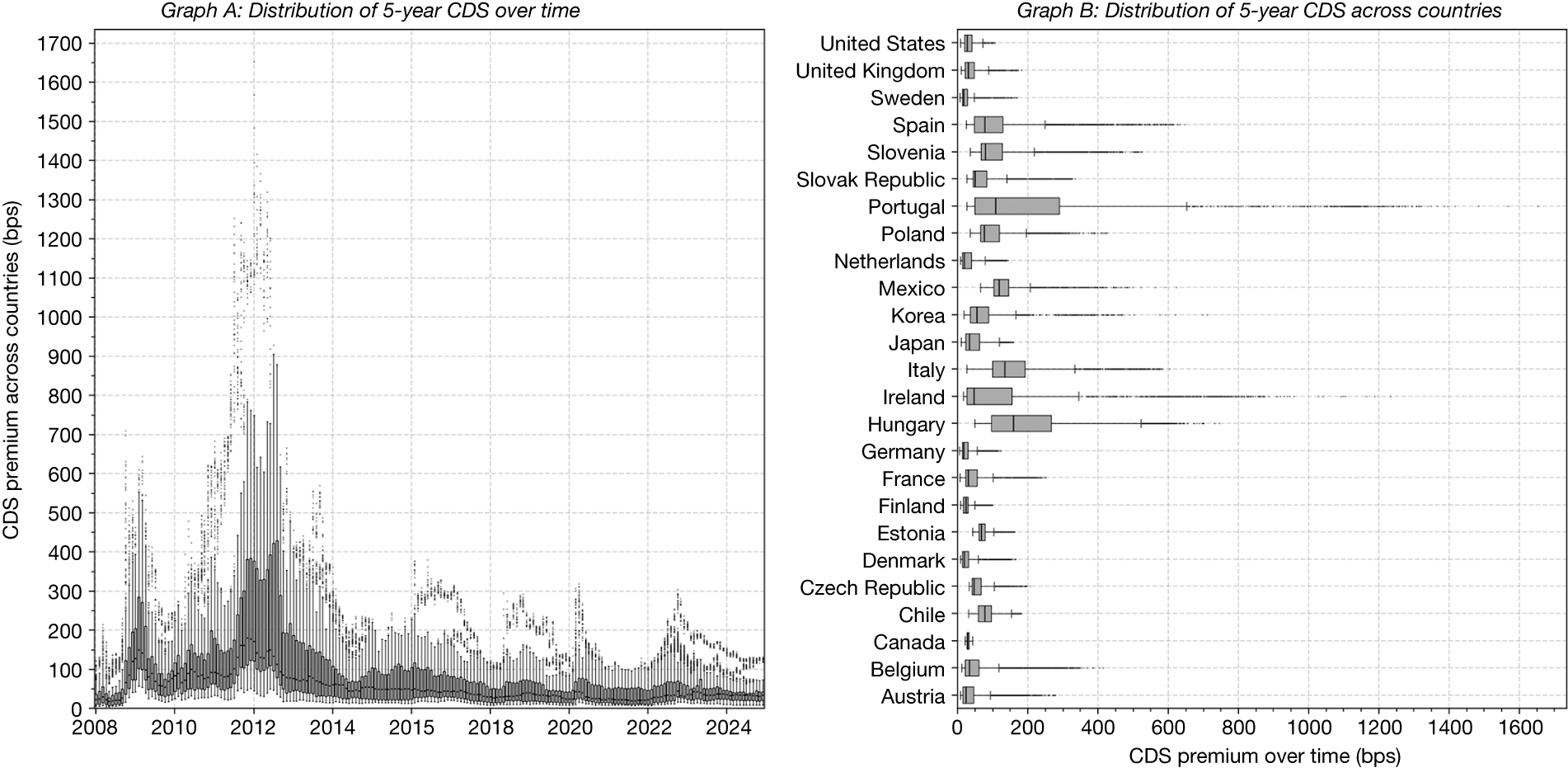
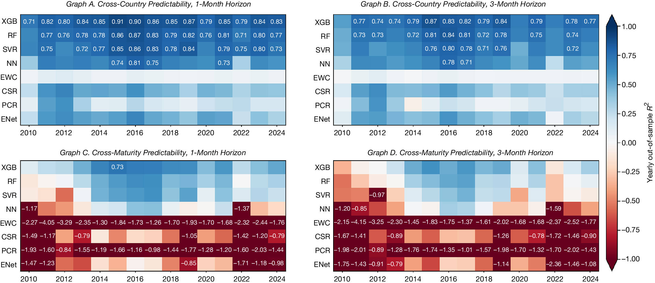


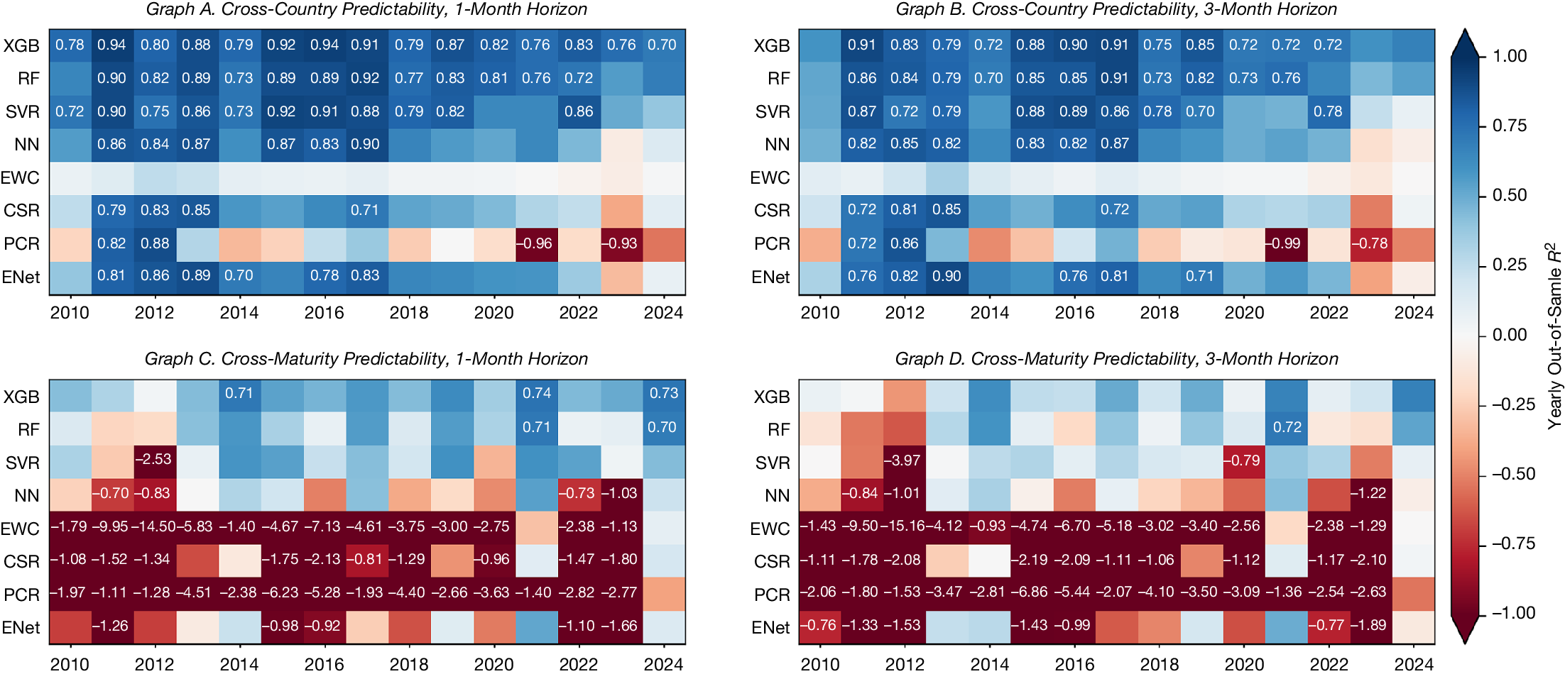


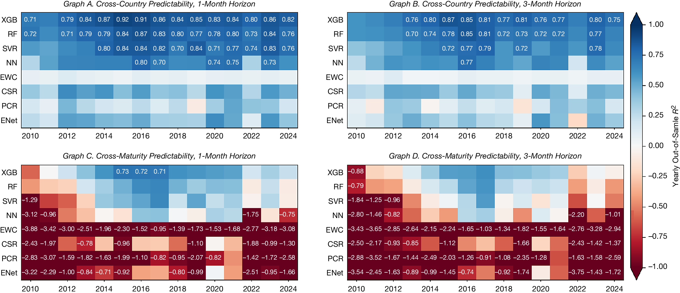


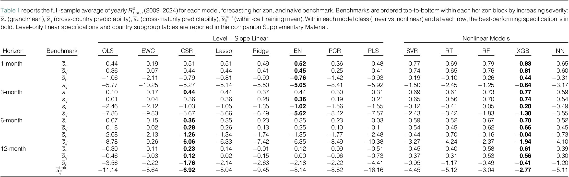

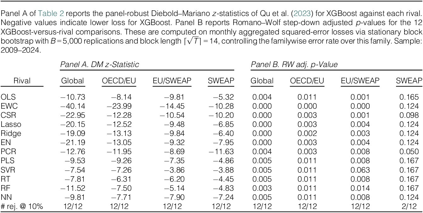
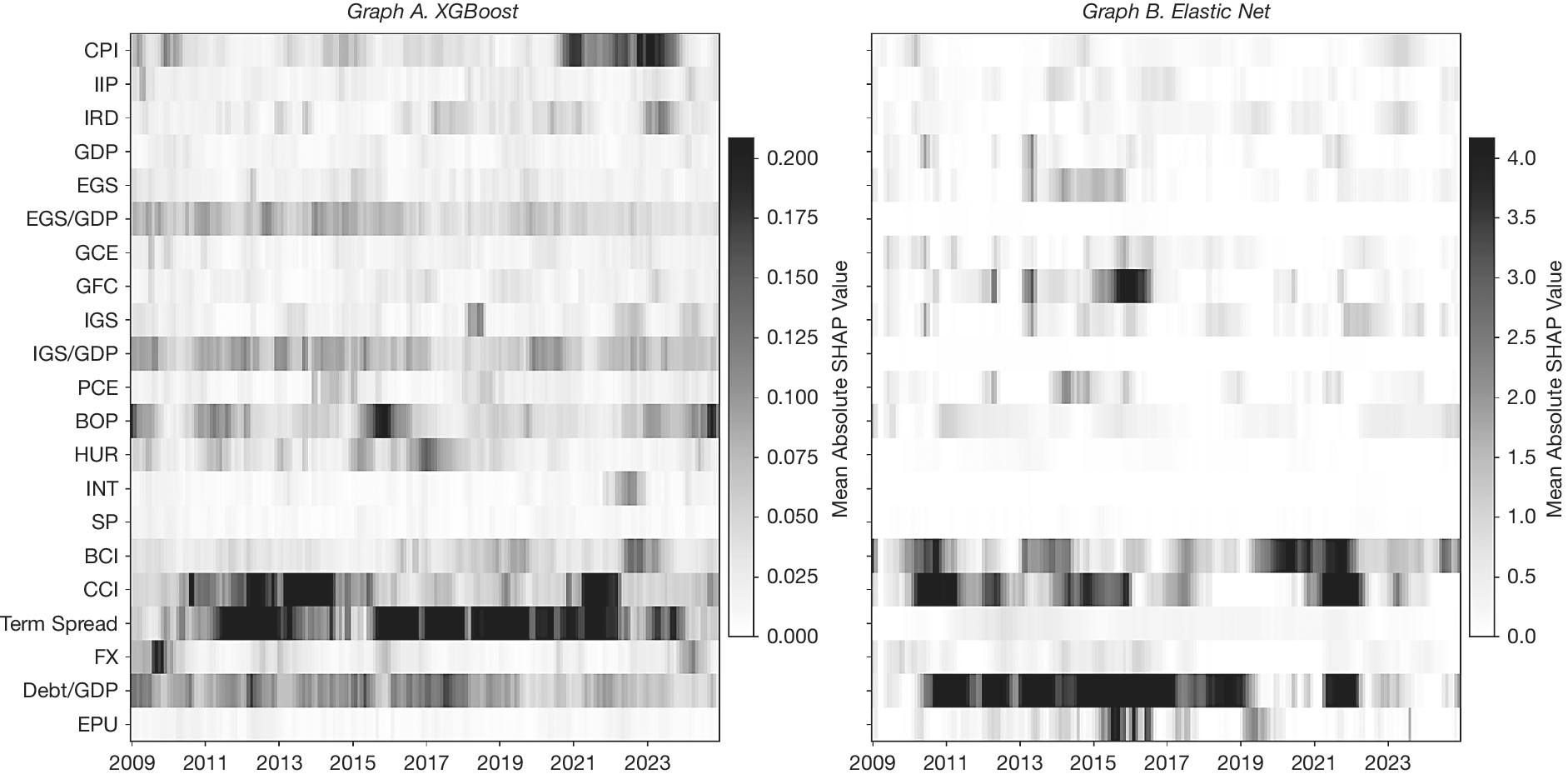
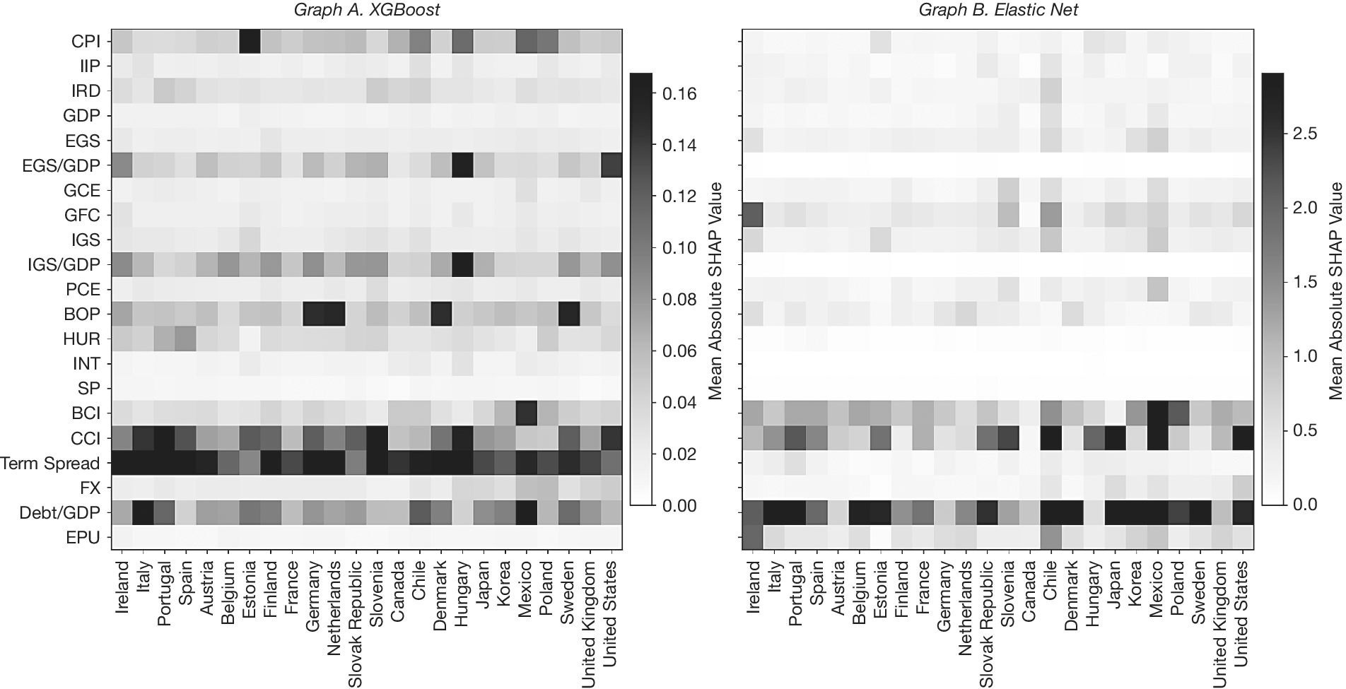
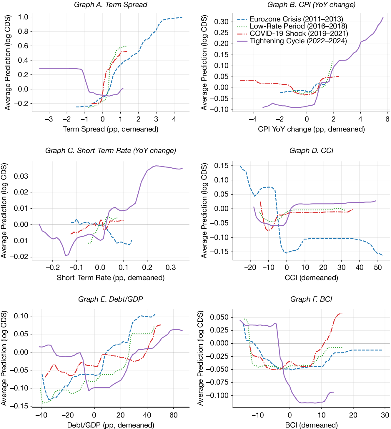
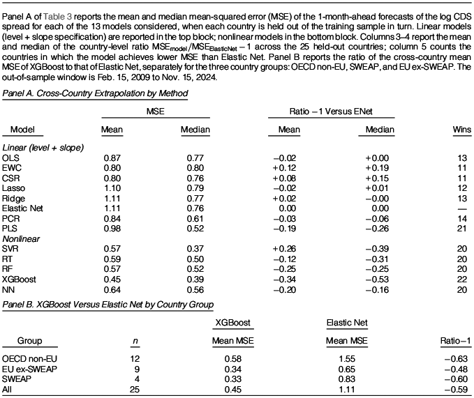
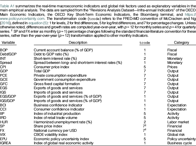
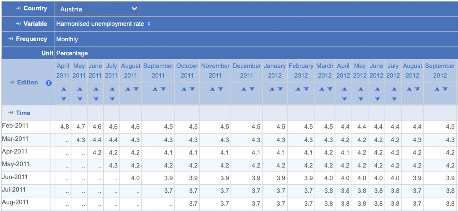

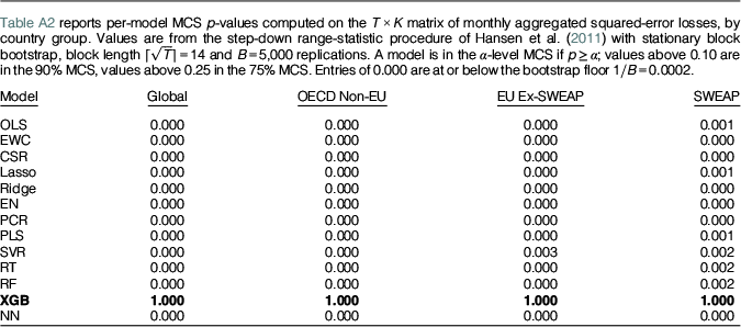

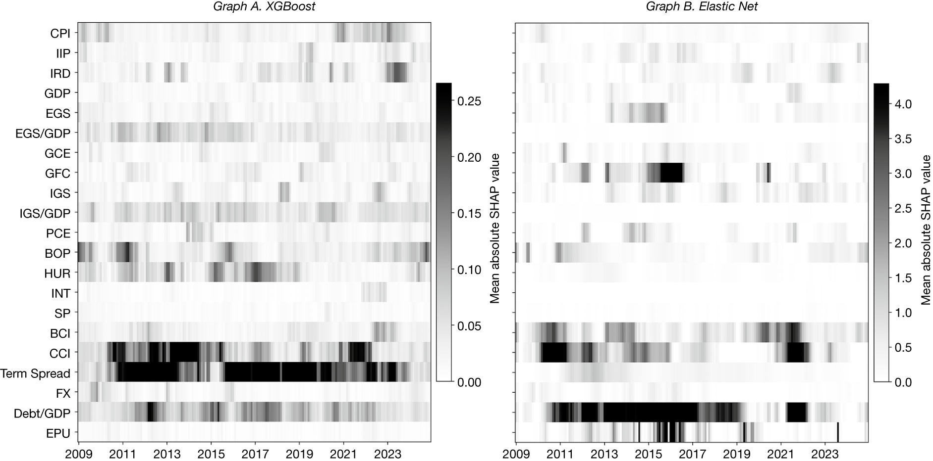
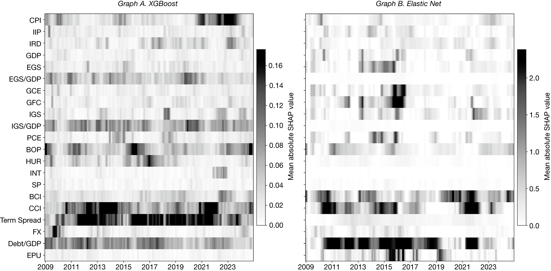
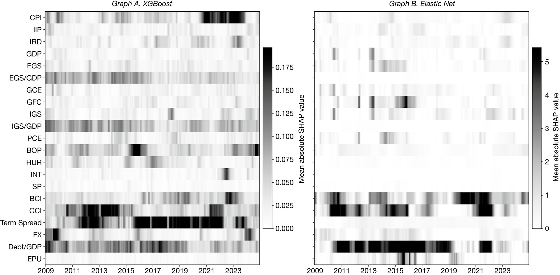


 Open access

