


1. Introduction
Turbulent thermally driven convection flows are frequently encountered in many geophysical and industrial situations. The vertical natural convection boundary layer (NCBL), among one of the most common configurations, is sustained by a vertical heated (or, cooled) wall with the gravity perpendicular to the driving heat flux. The temperature difference between the vertical wall and the quiescent ambient flow causes the local inhomogeneity of the body force, termed buoyancy, which drives the fluid to move against (or in, if cooled) the direction of gravity.
In an early theoretical investigation, George & Capp (Reference George and Capp1979) decomposed the turbulent NCBL into two distinct parts: a near-wall constant heat flux layer, in which total heat flux across the layer is independent of distance from the heated wall; an outer region where the NCBL is dominated by turbulent transport and is identified as the bulk mean flow. The multilayer structure of the turbulent NCBL has been widely used and developed by a number of scaling studies. Versteegh & Nieuwstadt (Reference Versteegh and Nieuwstadt1999) studied the scaling behaviour of the mean statistics for a turbulent NCBL in a doubly infinite differentially heated vertical slot using direct numerical simulation (DNS). Based on a multilayer approach and an order-of-magnitude analysis, they suggested that the near-wall region of their vertical natural convection is governed by a balance of viscous stress and buoyancy force, while the outer turbulent flow is determined by the geometry of the channel. Hölling & Herwig (Reference Hölling and Herwig2005) theoretically investigated the mean profiles of a spatially developing NCBL. In their analysis, the turbulent NCBL is decomposed into a viscosity-influenced near-wall region and a fully turbulent outer bulk mean flow. By asymptotically matching the temperature gradient in the overlap region, they suggested both temperature and velocity profiles for the turbulent NCBL follow a log-law.
More recently, Wells & Worster (Reference Wells and Worster2008) theoretically investigated a spatially developing NCBL using the experimental measurements by Tsuji & Nagano (Reference Tsuji and Nagano1988). In their analysis, the NCBL is decomposed into a near-wall region and an outer plume-like region. By numerically integrating their two-layer model for the NCBL, Wells & Worster (Reference Wells and Worster2008) showed that the buoyancy force in the near-wall region becomes progressively less significant as the NCBL becomes more turbulent. Using the empirical relations for the forced turbulent boundary layers, Wells & Worster (Reference Wells and Worster2008) suggested the existence of two turbulent regimes for the spatially developing NCBL: at some moderate Grashof number, shear is negligible in the outer momentum balance and the NCBL is controlled by a buoyancy driven instability; whereas at sufficiently high Grashof number the inertia of the flow becomes important so that the NCBL is controlled by a shear driven instability instead of a buoyancy driven instability. Making use of the integral level modelling for bulk mean flow and the Reynolds analogy assuming constant Stanton number, Wells & Worster (Reference Wells and Worster2008) also suggested the Nusselt number of the NCBL follows a  $1/2$-power-law correlation with the Grashof number in this shear instability turbulent regime – higher than the empirical
 $1/3$-power-law correlation (Cheesewright Reference Cheesewright1968; Vliet & Liu Reference Vliet and Liu1969; Tsuji & Nagano Reference Tsuji and Nagano1988; Abedin, Tsuji & Hattori Reference Abedin, Tsuji and Hattori2009; Nakao, Hattori & Suto Reference Nakao, Hattori and Suto2017). Similar higher scaling exponent is also seen in an earlier theoretical study of Eckert & Jackson (Reference Eckert and Jackson1950), who modelled the mean temperature and velocity profiles with a
 $1/7$-power-law and thereby obtained a
 $0.429$-power-law for the Nusselt number scaling. Ng et al. (Reference Ng, Ooi, Lohse and Chung2017) reported a DNS study of a differentially heated NCBL in a periodic vertical slot. By conditionally averaging high-shear events on the wall, Ng et al. (Reference Ng, Ooi, Lohse and Chung2017) found the wall heat transfer in the high-shear regions follows a slightly higher
 $0.37$-power-law correlation with the Grashof number; whereas in the low-shear region a
 $0.34$-power-law scaling is obtained for the Nusselt number. The authors described a flow structure where the outer core of the channel is turbulent but the near-wall boundary layer was either laminar (in low-shear regions) or turbulent (in high-shear regions). The coupling of the near-wall behaviours with the outer flow produces the differing scalings. The authors also noted the
 $0.37$-power-law correlation appears consistent with the high Grashof number ultimate heat transfer (
 $1/2$-power-law correlation) with a logarithmic boundary layer correction (cf. Kraichnan Reference Kraichnan1962; Grossmann & Lohse Reference Grossmann and Lohse2011). Similar ideas have been well developed for Rayleigh–Bénard convection (e.g. Grossmann & Lohse Reference Grossmann and Lohse2000, Reference Grossmann and Lohse2001) where a bulk-dominated ultimate turbulent regime is thought to be achieved at very high Grashof numbers. Our previous work on the temporally developing NCBL in Ke et al. (Reference Ke, Williamson, Armfield, Norris and Komiya2020) also investigated the law of the wall in the near-wall region for the NCBL using DNS. That study showed that the mean temperature profile for the turbulent NCBL appears self-similar and follows a log-law; whereas such a log-law is modified for the mean streamwise velocity profile due to the additional buoyancy in the near-wall region, and that the near-wall buoyancy becomes increasingly weak such that the NCBL would be asymptotic to momentum-dominated behaviour in the limit of higher Grashof number. Unfortunately, further investigation on the fundamental mechanics and heat transfer characteristics for the turbulent NCBL has been limited due to a lack of experimental and numerical data at high Grashof numbers.
Direct measurements and analyses of the bulk mean flow for the vertical NCBL flow away from the wall are also lacking. Previous studies suggested the bulk mean flow of the turbulent NCBL may be modelled using an integral modelling approach following Morton, Taylor & Turner (Reference Morton, Taylor and Turner1956). Wells & Worster (Reference Wells and Worster2008) suggested the bulk mean flow is characterised by the velocity and length scales similar to those of an integral plume model developed by Morton et al. (Reference Morton, Taylor and Turner1956) and those of the filling box measurements by Cooper & Hunt (Reference Cooper and Hunt2010). Kerr & McConnochie (Reference Kerr and McConnochie2015) investigated the dissolution of a vertical ice wall into homogeneous salty water. The experimental investigation shows that mass transfer in the ice dissolution process, driven by turbulent compositional convection, is very similar to the heat transfer in turbulent NCBL flows, and the dissolving ice is found to be well modelled by a planar plume with a uniformly distributed source of buoyancy. Their work was later extended by McConnochie & Kerr (Reference McConnochie and Kerr2016), who experimentally investigated a turbulent wall plume driven by a uniformly distributed source of buoyancy. The authors showed that the turbulent NCBL measurements by Cheesewright (Reference Cheesewright1968) and Vliet & Liu (Reference Vliet and Liu1969) agree well with their ‘updated plume model’ when a linear velocity profile (or Gaussian in their appendix) is assumed. A similar study was reported by Gayen, Griffiths & Kerr (Reference Gayen, Griffiths and Kerr2016) who investigated the turbulent compositional convection during ice dissolution. Using DNS data, Gayen et al. (Reference Gayen, Griffiths and Kerr2016) showed their compositional convection boundary layer flow can be well described by the model of Cooper & Hunt (Reference Cooper and Hunt2010) with different prefactors, and the structure of the compositional convection boundary layer agrees well with both the vertical NCBLs and the wall plume with distributed buoyancy flux. The effect of source and boundary conditions (BCs) on the wall plumes with distributed buoyancy source are reviewed in Kaye & Cooper (Reference Kaye and Cooper2018). The above studies show that the turbulent NCBL and the turbulent planar (wall) plume, although different in flow conditions, may share similar governing mechanics and physics (such as self-similarity and entrainment). At present there is a lack of direct evidence for how the bulk mean flow behaves in an NCBL and to what extent this flow can be represented by integral level modelling in the sense of Morton et al. (Reference Morton, Taylor and Turner1956) and Cooper & Hunt (Reference Cooper and Hunt2010).
The present study follows our previous work in Ke et al. (Reference Ke, Williamson, Armfield, Norris and Komiya2020), where the near-wall dynamics of the temporally developing turbulent NCBL adjacent to a vertical isothermal wall was investigated. In the present study, we investigate the bulk mean flow (later identified as the plume-like region in § 3) of the turbulent NCBL in terms of the integral model framework outlined by Craske & van Reeuwijk (Reference Craske and van Reeuwijk2015). Using DNS data at high Grashof number, we further examine the characteristics of this plume-like region, and show how the near-wall heat transfer and skin friction is linked to the bulk flow. The use of a temporal framework allows DNS to achieve a higher Grashof number (more turbulent) NCBL flow with relatively less computational effort compared with the canonical spatially developing flows. The application of the periodic BCs at the streamwise and spanwise boundaries ensures a parallel, temporally developing flow and a greatly reduced computational domain size and grid resolution. This technique has also been adapted by a number of flows that are generally thought spatially developing (see e.g. Abedin et al. Reference Abedin, Tsuji and Hattori2009; Abedin, Tsuji & Hattori Reference Abedin, Tsuji and Hattori2010; Kozul, Chung & Monty Reference Kozul, Chung and Monty2016; Ke et al. Reference Ke, Williamson, Armfield, McBain and Norris2019, Reference Ke, Williamson, Armfield, Norris and Komiya2020).
The paper is organised as follows. An overview and a mathematical description of the problem is given in § 2. In § 3, the boundary layer structure is discussed and the formulation of the integral modelling for the plume-like region of our temporally developing NCBL is derived. In § 4, we show the detailed analysis using an integral model for the plume-like region. The entrainment rate of the turbulent NCBL is discussed in § 4.3. The analytical solution to the self-similar integral model is derived in § 4.4, and implications for the heat transfer is discussed in § 4.5. In § 4.6, the physical consistency of the current heat transfer characteristics based on the integral model with the ultimate turbulent regime in the sense of Grossmann & Lohse (Reference Grossmann and Lohse2011) is discussed. Based on the force balance in the constant forcing region, the wall shear stress scaling is derived in § 4.7. Section 5 briefly summarises the findings in this paper.
2. Problem definition
The present study considers an incompressible turbulent NCBL adjacent to a vertical isothermal wall. The flow is governed by the conservation of mass, momentum and thermal energy. With the Boussinesq approximation, the governing equations in their dimensional form, read
 \begin{gather} \frac{\partial u_i}{\partial x_i} = 0, \end{gather}
 \begin{gather}\frac{\partial u_i}{\partial t}+\frac{\partial u_i u_j}{\partial x_j} ={-}\frac{1}{\rho}\frac{\partial p}{\partial x_i}+\nu\frac{\partial^2 u_i}{\partial {x_j}^2}+ g\alpha \theta\delta_{i1}, \end{gather}
 \begin{gather}\frac{\partial \theta}{\partial t}+\frac{\partial u_j \theta}{\partial x_j} = \kappa\frac{\partial^2 \theta}{\partial {x_j}^2}, \end{gather}
where subscripts  $i,j=1,2,3$ represent the
 $x$ (streamwise),
 $y$ (wall-normal) and
 $z$ (spanwise) axes, and the velocity field is given by
 $u_1, u_2, u_3 = u,v,w$. In (2.1),
 $\theta =T - T_\infty$ is the temperature (difference) field given by the local temperature
 $T$ and the far-field temperature
 $T_\infty$,
 $\rho$ is the density of the fluid,
 $\nu$ the kinematic viscosity of the fluid,
 $\kappa$ the thermal diffusivity of the fluid,
 $g$ is the gravitational vector pointing to the negative
 $x$ direction,
 $\alpha$ is the thermal expansion coefficient and
 $\delta _{i1}$ is the Kronecker delta (
 $\delta _{i1}=1$ if
 $i=1$ otherwise
 $\delta _{i1}=0$). The Prandtl number, given by the ratio of the fluid kinematic viscosity to the thermal diffusivity, is
 \begin{equation} \textit{Pr} \equiv\frac{\nu}{\kappa}=0.71. \end{equation}
The transient flow system (2.1), when subjected to a vertical isothermally heated wall, has a laminar analytical solution given by Illingworth (Reference Illingworth1950) and Schetz & Eichhorn (Reference Schetz and Eichhorn1962). For  $\textit {Pr}\neq 1$, velocity and temperature profiles are given in the dimensional form,
 \begin{gather} \theta = \theta_w \,\text{erfc}(\eta), \end{gather}
 \begin{gather}u = \frac{4g\alpha \theta_w t}{1-\textit{Pr}}\left[\text{i}^2\,\text{erfc}(\eta)-\text{i}^2\,\text{erfc}\left(\frac{\eta}{\sqrt{\textit{Pr}}}\right)\right] , \end{gather}
where  $\theta _w = T_w-T_\infty$ is the temperature difference between the isothermal wall
 $T_w$ and the ambient
 $T_\infty$,
 $\eta = y/\sqrt {4\kappa t}$ is a similarity parameter,
 $\text {erfc}(\eta )$ is the complementary error function of
 $\eta$ and
 $\text {i}^n\,\text {erfc}(\eta )$ represents the
 $n$th integral of the complementary error function with respect to
 $\eta$.
The boundary layer thickness is defined by an integral velocity thickness,
 \begin{equation} \delta \equiv \int^{\infty}_{0} \frac{\bar u}{\bar{u}_m} \,\mathrm{d} y, \end{equation}
where  $\bar {(\cdot )}$ denotes the mean (spatial average) value over the homogeneous (
 $x$–
 $z$) plane and
 $\bar {u}_m$ represents the maximum streamwise mean velocity. The instantaneous Grashof number based on the integral velocity thickness is therefore defined by
 \begin{equation} \textit{Gr}_\delta \equiv \frac{g\alpha \theta_w\delta^3}{\nu^2}. \end{equation}
Unlike the spatially developing NCBL flows, (2.4) and (2.5) do not vary with the downstream distance  $x$ due to the parallel nature of the flow, but depend solely on time
 $t$ since the NCBL is unsteady, i.e.
 $\delta (t)$ and
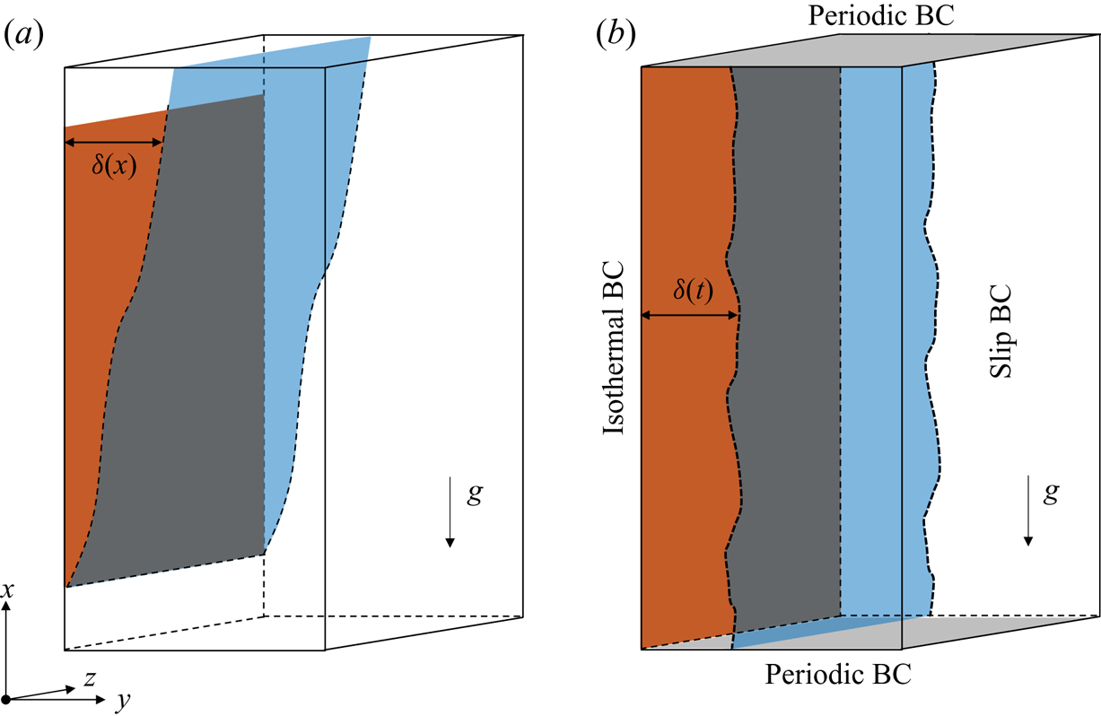
 $\textit {Gr}_\delta (t)$. Figure 1 depicts the difference between the canonical spatially developing NCBL and the temporally developing NCBL. The DNS results of the present study are compared with the spatially developing NCBL by matching
 $\textit {Gr}_\delta$ as in our previous work in Ke et al. (Reference Ke, Williamson, Armfield, Norris and Komiya2020). This method has also been used by Abedin et al. (Reference Abedin, Tsuji and Hattori2009) in a turbulent temporally developing NCBL study.
The systematic sketch (not to scale) of (a) a spatially developing NCBL, the boundary layer grows with downstream distance  $\delta (x)$ (e.g. Tsuji & Nagano Reference Tsuji and Nagano1988) and (b) a temporally developing NCBL, the boundary layer grows with time
 $\delta (t)$ (present study).

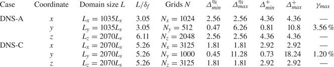
The governing equations (2.1) are discretised in an  $L_x\times L_y\times L_z$ computational domain using a finite volume method with a fourth-order spatial discretisation for the nonlinear advection terms and second-order discretisations for all other spatial terms. Uniform grids are used in the homogeneous directions, whereas a logarithmically stretched mesh (with a maximum stretching rate of
 $\gamma _{max}$) is applied in the wall-normal direction. The temporal integration of the flow is approximated by a hybrid discretisation – an explicit Adams–Bashforth method is used for the advection terms and the implicit Crank–Nicolson differencing is adopted for the diffusive terms. The code has previously been used in a number of natural convection publications (Williamson, Armfield & Kirkpatrick Reference Williamson, Armfield and Kirkpatrick2012; Ke et al. Reference Ke, Williamson, Armfield, McBain and Norris2019, Reference Ke, Williamson, Armfield, Norris and Komiya2020). It is also convenient to introduce the intrinsic length and velocity scales in order to describe the details of the numerical set-up and results, given by
 \begin{equation} L_s = \kappa^{2/3}/(g\alpha \theta_w)^{1/3}, \quad U_s = (\kappa g \alpha \theta_w)^{1/3}. \end{equation}
The intrinsic scales are chosen since the NCBL is both vertically (streamwise) and transversely (spanwise) unbounded, which yields no natural length scale for the flow. The use of the intrinsic scales given in (2.6) provides a normalisation of the flow quantities independent of the flow regime. A detailed description of the mesh strategy for the current study is shown in table 1. Note that in table 1,  $\eta _k$ refers to the smallest the Kolmogorov scale (i.e. first grid adjacent to the wall) after taking the spatial average in the homogeneous
 $x$–
 $z$ plane.
Grid and domain sizes of the simulations. The domain sizes are represented in the intrinsic length scale ( $L_s$) and the boundary layer thickness at the end of that simulation (
 $\delta _f$). The grid size in Kolmogorov scale,
 ${\varDelta ^{\eta _k}}$, and the grid size in wall units,
 ${\varDelta ^{+}}$, where the subscript
 $min$ represents the smallest grid (first grid adjacent to the wall) and
 $max$ represents the largest grid (far field) for the largest
 $\textit {Gr}_\delta$ achieved in that simulation,
 $\gamma _{max}$ represents the maximum stretching rate. Case DNS-A has also been reported in Ke et al. (Reference Ke, Williamson, Armfield, Norris and Komiya2020).

The temporally developing (spatially invariant) parallel flow is obtained by imposing the periodic BCs in the homogeneous ( $x$ and
 $z$) directions. The velocity is set to zero on the non-slip and non-permeable isothermal wall whereas a slip wall BC is applied in the far-field. Numerically, the BCs are expressed by
 \begin{gather} u=v=w=0,\quad \theta = \theta_w,\quad \text{at }y=0, \end{gather}
 \begin{gather}\frac{\partial u}{\partial y}=v=\frac{\partial w}{\partial y}=\theta=0, \quad \text{at }y=\infty. \end{gather}
The far-field boundary at  $y=\infty$ is replaced by the domain size
 $y=L_y$ in the simulation.
For DNS-A, the initial condition of the NCBL is prescribed by the laminar analytical solution given in (2.3) at an initial Grashof number of  $\textit {Gr}_\delta =3000$. The initial temperature field is augmented with streamwise and spanwise perturbation,
 \begin{equation} \theta_0 = \bar{\theta}(y) + \tilde{\theta}_x + \tilde{\theta}_z, \end{equation}
where  $\bar {\theta } (y)$ is the laminar analytical solution given by (2.3a), and
 $\tilde {\theta }_x$ and
 $\tilde {\theta }_z$ are the temperature fluctuations given by
 \begin{gather} \tilde{\theta}_x = \bar{\theta}(y)A_x\sum_{r=0}^{7}\sin\left(2^r\frac{2{\rm \pi} x}{L_x}\right), \end{gather}
 \begin{gather}\tilde{\theta}_z = \bar{\theta}(y)A_z\sin\left(\frac{2{\rm \pi} n_z z}{L_z}\right). \end{gather}
Here,  $A_x=A_z=10^{-3}$ represent the magnitudes of the streamwise
 $\tilde {\theta }_x$ and spanwise
 $\tilde {\theta }_z$ temperature perturbations,
 $r$ is an integer specifying the sinusoidal components of
 $\tilde {\theta }_x$, whilst
 $n_z=23$ is an integer specifying the wavenumber for
 $\tilde {\theta }_z$. The data of DNS-A has also been reported previously in Ke et al. (Reference Ke, Williamson, Armfield, Norris and Komiya2020).
In order to achieve a higher  $\textit {Gr}_\delta$ while minimising the computational effort, case DNS-C is initialised in the turbulent regime using the DNS-A flow field at
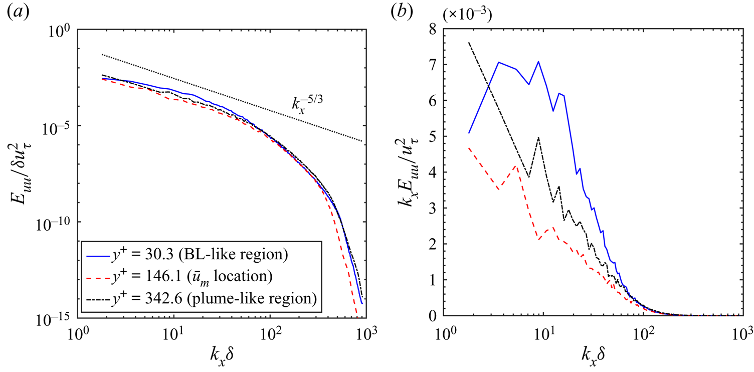
 $\textit {Gr}_\delta =5\times 10^7$. Figure 2(a) shows the streamwise velocity power spectrum
 $E_{uu}$ of case DNS-A at
 $\textit {Gr}_\delta =5\times 10^7$ with
 $y^+ = 30$ (inside the boundary layer-like (BL-like) region, see later in § 3),
 $y^+=146$ (the peak velocity location) and
 $y^+=343$ (the plume-like region, see also in § 3), where
 $k_x$ is the streamwise wavenumber. Evidently, the flow field at
 $\textit {Gr}_\delta =5\times 10^7$ is sufficiently turbulent to demonstrate a
 $k_x^{-5/3}$ power-law of the velocity spectrum for
 $y^+=146$ and
 $y^+=343$ at intermediate range of wavenumbers (inertial subrange). The turbulent structure at
 $\textit {Gr}_\delta =5\times 10^7$ is further examined in the premultiplied streamwise velocity spectrum, as shown in figure 2(b). The premultiplied spectrum has a local peak at
 $3< k_x\delta <9$ for
 $y^+=30$, indicating the domain size is large enough and the large scale motions are not contributing significantly to the streamwise turbulent energy in the near-wall (BL-like) region. However, due to computational limitations such a peak is absent farther away from the wall (
 $y^+=146$ and
 $y^+=343$) as the energy-containing structure continue to grow in size in the wall-normal direction. With increasing
 $\textit {Gr}_\delta$ the NCBL flow becomes more turbulent, requiring the DNS to have a larger domain size to accommodate the growing integral length scale and a finer finite volume mesh to resolve the diminishing small motions characterised by the Kolmogorov length scale. Although longer wavelength structures may lead to changes of the near-wall behaviour (Tsuji, Nagano & Tagawa Reference Tsuji, Nagano and Tagawa1992), truncated domains have been shown efficient to capture the near-wall statistics with good accuracy (Del Alamo et al. Reference Del Alamo, Jiménez, Zandonade and Moser2004; Lozano-Durán, Adrián, Jiménez Reference Lozano-Durán and Jiménez2014; MacDonald et al. Reference MacDonald, Chung, Hutchins, Chan, Ooi and García-Mayoral2017). Nevertheless, in § 4 we will show that the profile coefficients and other results for the integral model are insensitive to the large wavelengths and appear independent of the domain sizes considered.
The (a) power spectrum  $E_{uu}$ and (b) the premultiplied power spectrum
 $k_x E_{uu}$ of the streamwise velocity normalised by the friction velocity
 $u_\tau$ and the boundary layer thickness
 $\delta$ at
 $\textit {Gr}_\delta =5\times 10^7$ for case DNS-A. The dotted black line in panel (a) indicates the
 $k_x^{-5/3}$ power-law decay.

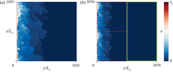
The application of the periodic BCs in the homogeneous directions allows us to duplicate the flow field of DNS-A in these directions so that a larger computational domain can be obtained. In the present study, we have doubled the streamwise and wall-normal domain size for DNS-C. The streamwise domain is filled with interpolated copies of the flow field obtained from DNS-A, so that
 \begin{align} \underbrace{\varphi(x,y,z)=\varphi(x+1035L_s,y,z)}_{\textit{DNS-C}} = \underbrace{\mathcal{G}[\varphi(x,y,z)]}_{\textit{DNS-A}},\quad \text{for }x\leq 1035L_s \text{ and } y\leq1035L_s, \end{align}
where  $\varphi =(u,v,w,\theta,p)$ denotes the flow variable and
 $\mathcal {G}$ is an interpolation function; whereas the increased wall-normal domain (
 $y>1035L_s$) is filled with ambient flow conditions (
 $\varphi =0$), see figure 3. A cubic interpolation is used to interpolate the initial flow field from a relatively coarse mesh (DNS-A) into a finer finite volume grid (DNS-C). We will show later in § 4 that the data from DNS-C demonstrates excellent collapse onto DNS-A in the range
 $5\times 10^7<\textit {Gr}_\delta <7\times 10^7$, i.e. the range extending from the initial condition of DNS-C to the largest
 $\textit {Gr}_\delta$ on DNS-A.
Initialising the temperature field of the turbulent NCBL for case DNS-C. (a) The temperature field obtained from DNS-A at  $\textit {Gr}_\delta =5\times 10^7$ (midspan,
 $z=1035L_s$). (b) The initialised temperature field for DNS-C at
 $\textit {Gr}_\delta =5\times 10^7$ (midspan,
 $z=1035L_s$). The red dashed box indicates duplicates of panel (a) and the green box indicates the ambient condition.

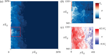
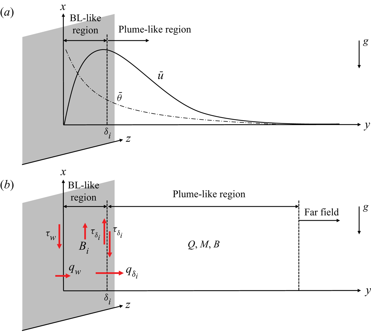
A flow field visualisation of the turbulent NCBL from DNS-C is given in figure 4(a) with a magnified view shown in figure 4(b,c). The visualisation shows a two-layer structure for the turbulent NCBL that has been previously reported by studies on wall bounded buoyancy driven flows (George & Capp Reference George and Capp1979; Wells & Worster Reference Wells and Worster2008; McConnochie & Kerr Reference McConnochie and Kerr2016). In the present study, we examine the flow physics of the near-wall region and the outer plume-like region separately – the flow is bounded by the isothermal wall in the near-wall region and a boundary-layer-like (BL-like) flow is developed, whereas farther away from the wall the NCBL depends on the vertical bulk mean flow and a plume-like region is developed. Following this convention, we define the BL-like and plume-like regions by a wall-normal distance  $\delta _i$ (BL–plume interface), as shown in the systematic sketch in figure 5(a). The BL-like region, as shown in figure 5(b), is driven by the buoyancy force
 $B_i$ within the region and the shear stress
 $\tau _{\delta _i}$ supplied by the plume-like region. The sum of the two driving forces in the BL-like region balances the shear stress on the wall
 $\tau _w$ and the acceleration. However, the plume-like region is controlled by the BCs (for example, shear
 $\tau _{\delta _i}$ and heat
 $q_{\delta _i}$) supplied by the BL-like region on the BL–plume interface
 $y=\delta _i$. The DNS data allows us to determine how integral level modelling approaches may be applied to this flow with the total flow rate (volume flux)
 $Q$, momentum
 $M$ and buoyancy
 $B$.
Visualisation of the midspan flow field for DNS-C at  $\textit {Gr}_\delta =1.2\times 10^8$: (a) temperature contours; (b) magnified temperature contours of the red box in panel (a); (c) magnified velocity contours of the red box in panel (a). The dashed line indicates the maximum streamwise velocity location
 $\delta _m=38.85L_s$.

Systematic sketch of (a) the mean profiles and (b) the BL-like region and plume-like region of the NCBL (not to scale).

3. Integral model formulation
The integral equations for plumes (Morton et al. Reference Morton, Taylor and Turner1956) have been successfully used to model the turbulent NCBLs (e.g. Wells & Worster Reference Wells and Worster2008; McConnochie & Kerr Reference McConnochie and Kerr2016).
The integral model is derived from the streamwise momentum Reynolds-averaged Navier–Stokes (known as RANS) and the conservation equations of thermal energy which, in dimensional form, read
 \begin{gather} \frac{\partial \bar u}{\partial t} + \frac{\partial \overline{u'v'}}{\partial y} = \nu\frac{\partial^2 \bar u}{\partial y^2} + \bar b, \end{gather}
 \begin{gather}\frac{\partial \bar b}{\partial t} + \frac{\partial \overline{v'b'}}{\partial y} = \kappa\frac{\partial ^2 \bar b}{\partial y^2} , \end{gather}
where the buoyancy source  $b = g\alpha \theta$, and
 $\bar {\varphi }$ denotes the spatial ensemble average of flow quantity
 $\varphi$ over the homogeneous (
 $x$–
 $z$) plane, such that
 $\varphi = \bar \varphi + \varphi '$ according to Reynolds decomposition. It is noted that since the periodic BCs are imposed in the streamwise and spanwise directions, the spatial derivatives in the homogeneous directions and the mean wall-normal velocity must vanish, i.e.
 $\partial \bar \varphi /\partial x = \partial \bar \varphi /\partial z= \bar v = 0$. Consequently, for a planar temporally evolving flow the continuity equation (2.1a) vanishes. In the present study, we follow the integral framework outlined by van Reeuwijk & Craske (Reference van Reeuwijk and Craske2015), and employ the mean streamwise kinetic energy equation. Such an integral framework is consistent with the conservation equations in (2.1) and has been used in a number of free shear flow studies (e.g. Craske & van Reeuwijk Reference Craske and van Reeuwijk2015; Krug et al. Reference Krug, Chung, Philip and Marusic2017). The mean streamwise kinetic energy is obtained by multiplying the streamwise momentum equation (3.1a) by
 $2\bar u$, as follows:
 \begin{equation} \frac{\partial {\bar{u}}^2 }{\partial t} + 2 \frac{\partial \overline{u'v'}\cdot\bar u}{\partial y} - 2\overline{u'v'}\frac{\partial \bar u}{\partial y} = \nu \frac{\partial^2 {\bar u}^2}{\partial y^2} - 2 \nu\left( \frac{\partial \bar u}{\partial y}\right)^2 +2\bar u \bar b. \end{equation}
Considering the plume-like region of system (3.1)–(3.2) at an integral level, the plume-like region can be described by the integral quantities: volume flux  $Q$, the integral buoyancy
 $B$ and the momentum flux
 $M$ of the plume-like region of the turbulent boundary layer. These integral quantities are defined as
 \begin{equation} Q \equiv\int^\infty_{\delta_i} \bar u \,\mathrm{d} y, \quad B \equiv \int^\infty_{\delta_i} \bar b \,\mathrm{d} y, \quad M \equiv \int^\infty_{\delta_i} {\bar u }^2 \,\mathrm{d} y, \end{equation}
where the plume-like region of the turbulent boundary layer is defined by  $\delta _i\leq y < \infty$ (see figure 5). Based on the integral quantities (3.3), characteristic velocity, width and buoyancy scales are obtained as
 \begin{equation} \hat{u}=\frac{M}{Q},\quad\hat{l}=\frac{Q^2}{M},\quad\hat{b}=\frac{BM}{Q^2}. \end{equation}
The following integral model analysis does not require a profile shape to be defined (e.g. van Reeuwijk & Craske Reference van Reeuwijk and Craske2015). The integral equations for the plume-like region of the unsteady turbulent NCBL are obtained by integrating (3.1) and (3.2) from  $\delta _i$ to the far field, with the far field BCs
 \begin{equation} \overline{u'v'}=\overline{v'b'}=\frac{\partial \bar u}{\partial y}=\bar b=0, \quad \text{when}\ y\rightarrow \infty. \end{equation}
Making a substitution of (3.3), the integral equations now read
 \begin{gather} \frac{\partial Q}{\partial t} = B - {\hat{u}^2}(S_{\delta_i}+\mathcal{L}_Q), \end{gather}
 \begin{gather}\frac{\partial B}{\partial t} = {\hat{u}\hat{b}}(\beta_{\delta_i}-\mathcal{L}_B), \end{gather}
 \begin{gather}\frac{\partial M}{\partial t} = \hat{u}^3(M_{\delta_i}+\varSigma_M - \mathcal{L}_M). \end{gather}
Here,  $S_{\delta _i}$,
 $\beta _{\delta _i}$ and
 $M_{\delta _i}$ are the normalised shear, buoyancy (heat) and integral production BCs at
 $y=\delta _i$, given by
 \begin{gather} {S_{\delta_i}}= \frac{\tau_{\delta_i}}{\hat{u}^2}= \frac{1}{\hat{u}^2} \left( \nu \frac{\partial \bar u}{\partial y}-\overline{u'v'} \right)_{y=\delta_i}, \end{gather}
 \begin{gather}\beta_{\delta_i}= \frac{g\alpha q_{\delta_i}}{\hat{u}\hat{b}} = \frac{1}{\hat{u}\hat{b}}\left( -\kappa\frac{\partial \bar b}{\partial y}+\overline{v'b'} \right)_{y=\delta_i}, \end{gather}
 \begin{gather}M_{\delta_i}=\frac{\varPi_{\delta_i}}{\hat{u}^3} =\frac{2}{\hat{u}^3}( \overline{u'v'} \cdot \bar u )_{y=\delta_i}, \end{gather}
where  $\tau _{\delta _i}$,
 $q_{\delta _i}$ and
 $\varPi _{\delta _i}$ are the corresponding dimensional BCs;
 $\mathcal {L}_Q$,
 $\mathcal {L}_B$ and
 $\mathcal {L}_M$ in (3.6) represent the dimensionless Leibniz term when taking the integral from
 $\delta _i$ to the far-field,
 \begin{gather} \mathcal{L}_Q = \frac{\bar{u}_{\delta_i}}{\hat{u}^2} \frac{\partial \delta_i}{\partial t}, \end{gather}
 \begin{gather}\mathcal{L}_B = \frac{\bar{b}_{\delta_i}}{\hat{u}\hat{b}} \frac{\partial \delta_i}{\partial t}, \end{gather}
 \begin{gather}\mathcal{L}_M = \frac{\bar{u}_{\delta_i}^2}{\hat{u}^3} \frac{\partial \delta_i}{\partial t}, \end{gather}
where  $\bar {u}_{\delta _i}$ and
 $\bar {b}_{\delta _i}$ are the mean streamwise velocity and temperature on the interface
 $y=\delta _i$ at time
 $t$. The profile coefficient
 $\varSigma _M$ in (3.6c) denote the individual contributions to the rate of change in the momentum flux normalised by the local characteristic scales,
 \begin{equation} \varSigma_M = \gamma_p+\gamma_d+\gamma_f+ \gamma_b \textit{Ri} \end{equation}
and  $\textit {Ri}$ is the Richardson number given by
 \begin{equation} \textit{Ri}=\frac{\hat{b}\hat{l}}{\hat{u}^2}=\frac{BQ^2}{M^2}. \end{equation}
Following the framework outlined by van Reeuwijk & Craske (Reference van Reeuwijk and Craske2015), these contributions are
 \begin{gather} \gamma_p = \frac{\varGamma_p}{\hat{u}^3}= \frac{2}{\hat{u}^3}\int^{\infty}_{\delta_i} \overline{u'v'}\frac{\partial \bar u}{\partial y} \,\mathrm{d} y , \end{gather}
 \begin{gather}\gamma_f = \frac{\varGamma_f}{\hat{u}^3} = \frac{ \nu}{\hat{u}^3}\int^{\infty}_{\delta_i} \frac{\partial^2 \bar{u}^2}{\partial y^2} \,\mathrm{d} y, \end{gather}
 \begin{gather}\gamma_d = \frac{\varGamma_d}{\hat{u}^3}={-}\frac{2 \nu}{\hat{u}^3}\int^{\infty}_{\delta_i} \left( \frac{\partial \bar u}{\partial y}\right)^2 \mathrm{d} y, \end{gather}
 \begin{gather}\gamma_b = \frac{\varGamma_b}{\hat{u}\hat{l}\hat{b}}= \frac{2}{\hat{u}\hat{l}\hat{b}}\int^{\infty}_{\delta_i} \bar u \bar b\,\mathrm{d} y, \end{gather}
where  $\gamma _p$ is the integral of the turbulence shear production in the plume-like region,
 $\gamma _f$ is the integral of the mean kinetic energy (MKE) diffusion,
 $\gamma _d$ the integral of the MKE dissipation, and
 $\gamma _b$ the buoyancy contribution to the MKE. The temporally developing parallel flow greatly simplifies the profile coefficients (cf. van Reeuwijk & Craske Reference van Reeuwijk and Craske2015), as shown in (3.6), since the gradients vanish in the homogeneous directions. The profile coefficients (3.11), together with the BCs (3.7), are expected to be constants (or, negligibly small otherwise) if the flow statistics appear self-similar in the outer part of the NCBL since they are normalised by the local characteristic scales
 $\hat {u}$,
 $\hat {l}$ and
 $\hat {b}$.
A similar approach was used by van Reeuwijk & Craske (Reference van Reeuwijk and Craske2015) and Craske & van Reeuwijk (Reference Craske and van Reeuwijk2016) for spatially developing unsteady jets and plumes and Krug et al. (Reference Krug, Chung, Philip and Marusic2017) for a planar temporally evolving plume, in which cases the total buoyancy flux is conserved within the flow, such that  $\partial B/\partial t = 0$; whereas in the present study, the plume-like region of the flow receives heat (and thus buoyancy) continuously from the BL-like region due to the presence of the isothermal wall. It is noted that in contrast to the previous studies of jets and plumes (van Reeuwijk & Craske Reference van Reeuwijk and Craske2015; Craske & van Reeuwijk Reference Craske and van Reeuwijk2016; Krug et al. Reference Krug, Chung, Philip and Marusic2017) where the wall is absent or (and) high Reynolds number flows are assumed to neglect the viscous effects, the viscous terms (3.11b) and (3.11c) are retained in the present NCBL study. However, we will see later in §§ 4.2 and 4.3 that such viscous effects are still negligibly small in the turbulent NCBL (in the presence of the wall) when compared with the dominant term.
4. Results and discussion
4.1. BL–plume interface
Before proceeding to a detailed analysis of the integral model (3.6), a rigorous definition of the BL–plume region interface,  $\delta _i$, is required. Since the flow is driven by buoyancy, we use the heat transfer characteristics to identify the different mechanics of the BL-like and plume-like region of the boundary layer. For the vertical NCBL flow, heat is supplied by the isothermal wall and is conducted away from the wall through molecular diffusion
 $-\rho c_p \kappa \partial \bar \theta /\partial y$ and turbulent heat transport
 $\rho c_p \overline {v'\theta '}$. In our previous work (Ke et al. Reference Ke, Williamson, Armfield, Norris and Komiya2020), a constant heat flux layer, in which region the total transport of heat
 $\mathcal {Q}$ is approximately constant, such that
 \begin{equation} \mathcal{Q}\equiv \rho c_p \left(\overline{v'\theta'}-\kappa \frac{\partial \bar \theta}{\partial y}\right) =\mathcal{Q}_w, \end{equation}
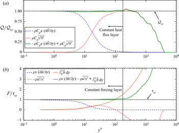
has been identified for the temporally developing NCBL up to  $\textit {Gr}_\delta =7.7\times 10^7$. The constant heat flux layer is consistent with the previous studies for turbulent spatially developing NCBLs (George & Capp Reference George and Capp1979; Hölling & Herwig Reference Hölling and Herwig2005; Wells & Worster Reference Wells and Worster2008). Here, the heat flux on the wall is given by
 \begin{equation} \mathcal{Q}_w ={-}\rho c_p \kappa \left.\frac{\partial \bar \theta}{\partial y}\right\rvert_{y=0}, \end{equation}
and  $c_p$ is the specific heat of the fluid. In the present study, such a constant heat flux layer is found for
 $y/L_s<40$ (or
 $y^+<180$ in wall units) at
 $\textit {Gr}_\delta =1.21\times 10^8$ for DNS-C, as demonstrated by figure 6(a). Figure 6(b) also depicts a constant forcing region in the vicinity of the isothermal wall as introduced by Ke et al. (Reference Ke, Williamson, Armfield, Norris and Komiya2020), so that the wall shear stress
 \begin{equation} {\tau}_w =\rho \nu \left.\frac{\partial \bar u}{\partial y}\right\rvert_{y=0}, \end{equation}
balances the local shear stress and the buoyancy force,
 \begin{equation} {\tau}_w = \rho\left( \nu\frac{\partial \bar u}{\partial y}-\overline{u'v'}\right)+\int_0^y \bar b \,\mathrm{d} y, \end{equation}
for  $y/L_s<40$ (
 $y^+<180$) at
 $\textit {Gr}_\delta = 1.21\times 10^8$. The existence of the constant flux and forcing layers given by (4.1) and (4.4) indicates that there exists a slowly varying region in the close vicinity of the wall where the acceleration of the flow has negligible influence on the dynamics.
Components of the (a) near-wall heat flux and (b) near-wall forcing in the near-wall region, showing the constant heat flux region and the constant momentum forcing region. Data obtained using DNS-C at  $\textit {Gr}_\delta =1.21\times 10^8$.

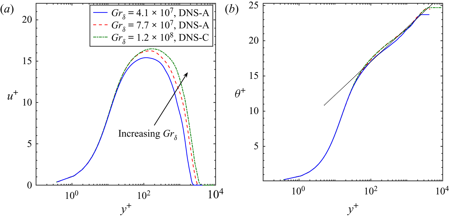
Figure 7 depicts the mean streamwise velocity and temperature profiles for the temporally developing NCBL for both DNS-A and DNS-C. The profiles are normalised in wall units, where
 \begin{equation} u^+\,{=}\, \frac{\bar{u}}{u_\tau}, \quad \theta^+\,{=}\, \frac{\theta_w-\bar{\theta}}{\theta_\tau}, \end{equation}
and  $u_\tau$,
 $\theta _\tau$ are the friction velocity and temperature, respectively, defined by
 \begin{equation} u_\tau = \sqrt{\frac{\tau_w}{\rho}},\quad \theta_\tau = \frac{\mathcal{Q}_w}{\rho c_p u_\tau}. \end{equation}
The mean streamwise velocity, as shown in figure 7(a), demonstrates a strong  $\textit {Gr}_\delta$ dependency due to the additional buoyancy effect and follows a modified log-law as suggested by Ke et al. (Reference Ke, Williamson, Armfield, Norris and Komiya2020), whereas the mean temperature, as shown in figure 7(b), appears independent of the
 $\textit {Gr}_\delta$ and features a temperature log-law (Tsuji & Nagano Reference Tsuji and Nagano1988; Ng et al. Reference Ng, Ooi, Lohse and Chung2017; Ke et al. Reference Ke, Williamson, Armfield, Norris and Komiya2020). In the present study, we identify the BL–plume interface
 $\delta _i$ to be the maximum mean streamwise velocity location for the results presented, i.e. the
 $y$ location at which
 $\bar {u}= \bar {u}_m$; this interface is found to be very close to the edge of the constant flux (and forcing) region. For instance, at
 $\textit {Gr}_\delta =1.2\times 10^8$ the BL–plume interface (
 $\bar {u}_m$ location) is located at
 $\delta _i^+ = 171.21$ in wall units; whereas the constant flux (and forcing) region extends up to
 $y^+\approx 180$. Nevertheless, in Appendix B, we revert the definition of
 $\delta _i$ to be the wall-normal location at which the molecular diffusion matches the turbulent heat flux (e.g. Wells & Worster Reference Wells and Worster2008), and the integral model is shown to be robust and insensitive to the exact definition of
 $\delta _i$, provided
 $\delta _i$ falls in the constant flux region.
The mean profiles of the temporally developing NCBL at different  $\textit {Gr}_\delta$ in wall units. (a) Mean streamwise velocity profile and (b) mean temperature profiles. The black dotted line in panel (b) indicates the logarithmic profile.

4.2. A self-similar model
Based on the definition of the BL–plume interface  $\delta _i$, the buoyancy BC for the integral model is then obtained by
 \begin{equation} \left.{g\alpha } {q}_{\delta_i}\equiv \left(-\kappa\frac{\partial \bar b}{\partial y}-\overline{v'b'}\right)\right\rvert_{y=\delta_i}\approx{g\alpha } {q}_w, \end{equation}
where  ${q} = \mathcal {Q}/{\rho c_p}$. The rate of change in the total buoyancy (3.6b) is therefore directly linked to the wall heat flux
 ${q}_w$,
 \begin{equation} \frac{\partial B}{\partial t} = \hat{u}\hat{b}(\beta_{\delta_i}-\mathcal{L}_B) ={g\alpha} {q}_{\delta_i} - \hat{u}\hat{b}\mathcal{L}_B={g\alpha } {q}_w- \hat{u}\hat{b}\mathcal{L}_B. \end{equation}
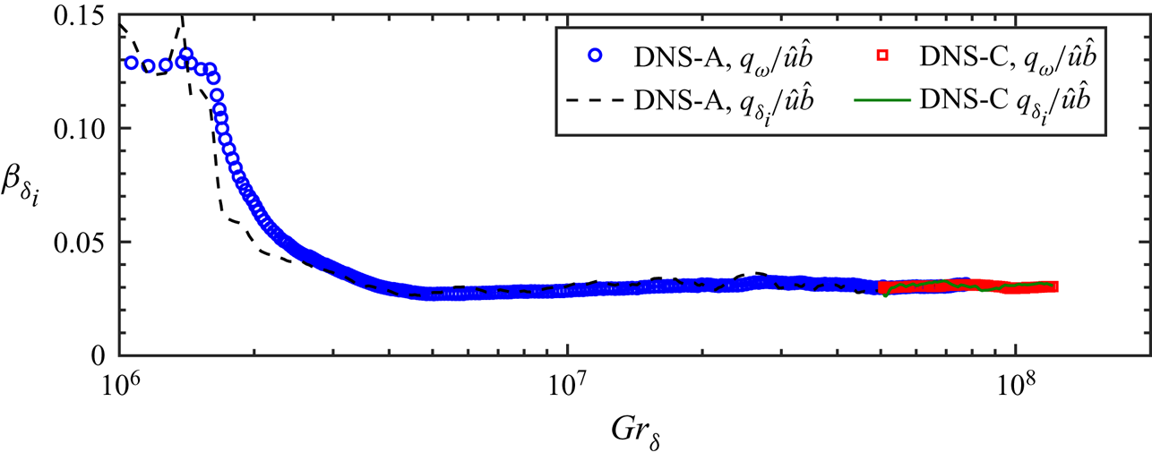
In the present study, the BCs of the integral model (3.7) are obtained by a linear interpolation of the DNS data onto the interface  $y=\delta _i$. Figure 8 demonstrates that
 $\beta _{\delta _i}$, being the dimensionless buoyancy BC for the integral model, is approximately constant for
 $\textit {Gr}_\delta >4\times 10^6$. This suggests that the heat flux through the interface
 $q_{\delta _i}$ scales with the local characteristic scales,
 \begin{equation} q_{\delta_i} \propto \hat{u}\hat{b}. \end{equation}
In addition, (4.7) and (4.9) further indicate that the heat flux on the wall scales with the plume-like region scales,
 \begin{equation} q_w\propto\hat{u}\hat{b}. \end{equation}
The implication of (4.10) is that the heat transfer of the turbulent NCBL on the wall is driven by the characteristic velocity and temperature scales in the plume-like region. As depicted by figure 8, the normalised wall heat flux shows excellent agreement with the buoyancy BC  $\beta _{\delta _i}$ and also appears constant for
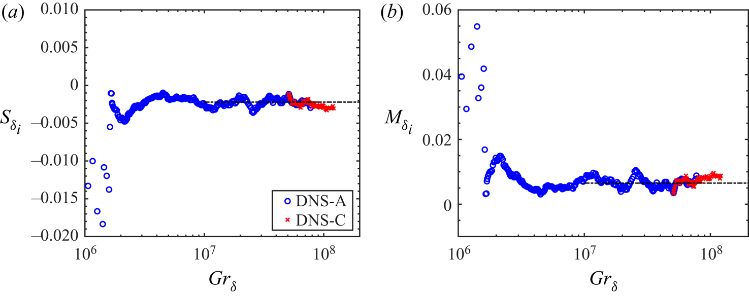
 $\textit {Gr}_\delta >4\times 10^6$. Similarly, the shear and integral production BCs for the integral model, scaled by the top-hat characteristic quantities, are shown in figure 9. It is clear that both BCs scale well with the characteristic scales since they are constants in the range
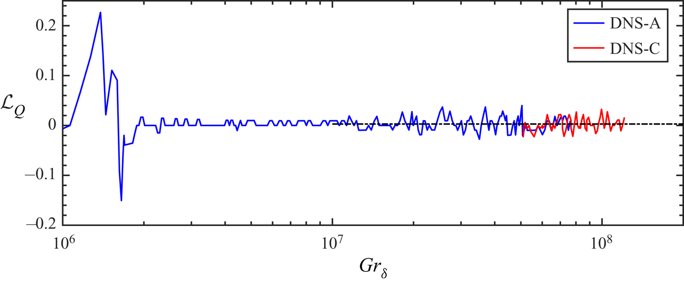
 $\textit {Gr}_\delta >10^7$. In addition, the dimensionless Leibniz terms are also appear constant in this Grashof number range. Figure 10 shows the temporal evolution of the Leibniz term
 $\mathcal {L}_Q$ for the volume flux
 $Q$. Evidently, in the fully turbulent regime
 $\mathcal {L}_Q$ appears constant with some level of temporal oscillation. The Leibniz terms for buoyancy
 $\mathcal {L}_B$ and momentum
 $\mathcal {L}_M$ (although not shown here) also demonstrate similar temporal fluctuations. Nevertheless, taking a temporal average for
 $\textit {Gr}_\delta >10^7$ yields
 $\mathcal {L}_Q\approx 0.0029$,
 $\mathcal {L}_B\approx 0.0041$ and
 $\mathcal {L}_M\approx 0.0042$. The constant Leibniz term
 $\mathcal {L}_Q$ further implies that the spreading rate of the interface
 $\partial \delta _i/\partial t$ scales with the velocity scale
 $\hat {u}^2/\bar {u}_m$. In the present study, the maximum streamwise velocity
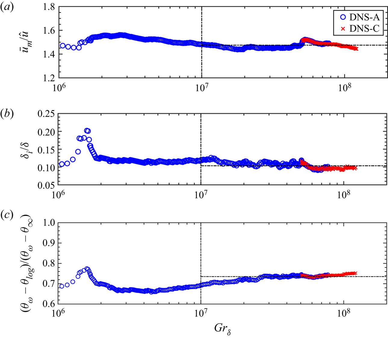
 $\bar {u}_m$ is found to scale with the characteristic velocity in the plume-like region (see, later in § 4.6), suggesting
 \begin{equation} \frac{\partial \delta_i}{\partial t} = E_1\hat{u} = E_2 \bar{u}_m, \end{equation}
where  $E_1$ and
 $E_2$ are the proportionality constants. Equation (4.11) takes a similar form to the entrainment relation (Morton et al. Reference Morton, Taylor and Turner1956), and may interpreted as the entrainment from the turbulent plume-like region to the near-wall BL-like region.
Temporal development of the dimensionless heat (buoyancy) BC  $\beta _{\delta _i}=g\alpha q_{\delta _i}/\hat {u}\hat {b}$ and the normalised wall heat flux
 $g\alpha q_w/\hat {u}\hat {b}$.

Normalised BCs for the integral model: (a) shear BC,  $S_{\delta _i} = \tau _{\delta _i}/\hat {u}^2$; (b) integral production BC,
 $M_{\delta _i} = \varPi _{\delta _i}/\hat {u}^3$. The black dash–dotted lines indicates the values listed in table 2.

The temporal development of the normalised Leibniz term  $\mathcal {L}_Q$ in (3.8). The black dash–dotted line indicates
 $\mathcal {L}_Q=0.0029$.

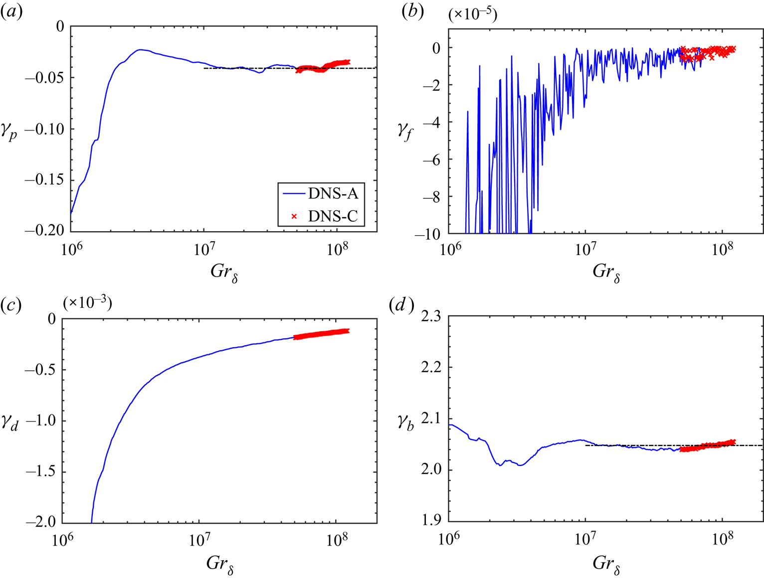
Profile coefficients for the integral model: (a) contribution of total shear production to the MKE,  $\gamma _p$; (b) contribution of viscous diffusion to the MKE,
 $\gamma _f$; (c) contribution of viscous dissipation to the MKE,
 $\gamma _d$; (d) contribution of buoyancy to the MKE,
 $\gamma _b$. The black dash–dotted lines indicates the values listed in table 2.

Profile coefficients of the integral model (3.6), shown in figure 11, are numerically obtained by integrating the DNS data from  $\delta _i$ to
 $L_y$. In figure 11, the profile coefficients
 $\gamma _p$ and
 $\gamma _b$ are clearly independent of
 $\textit {Gr}_\delta$ for
 $\textit {Gr}_\delta >10^7$, suggesting the plume-like region is self-similar; while the viscous terms
 $\gamma _d$ and
 $\gamma _f$ are of order
 $O(10^{-4})$ and
 $O(10^{-5})$, respectively, and gradually reducing in magnitude with increasing
 $\textit {Gr}_\delta$. The physical interpretation of figure 11 is straightforward: the bulk vigorous turbulent NCBL is accelerated and maintained by the buoyancy
 $\gamma _b$ while a small portion of the MKE is transferred to turbulent kinetic energy through shear production
 $\gamma _p$, and diffused
 $\gamma _f$ and dissipated
 $\gamma _d$ through viscosity. With increasing
 $\textit {Gr}_\delta$ the flow become more turbulent and the viscous effects diminish; while the driving buoyancy and shear remains significant at high
 $\textit {Gr}_\delta$ turbulent flow. It is noted that the buoyancy contribution
 $\gamma _b$ needs to be multiplied by
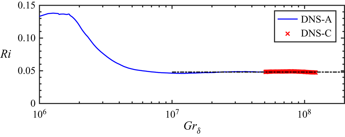
 $\textit {Ri}$ before it can be compared with the other three terms. In the present study, the Richardson number becomes a constant
 $\textit {Ri}\approx 0.048$ in the turbulent regime
 $\textit {Gr}_\delta >10^7$, as shown in figure 12, further supporting that the plume-like region of the turbulent NCBL is self-similar for
 $\textit {Gr}_\delta >10^7$. This indicates that the total buoyancy contribution to the MKE (
 $\gamma _b\textit {Ri}\approx 0.098$) is of leading order, while the viscous terms are negligible in the MKE balance as expected since the flow becomes more turbulent at high
 $\textit {Gr}_\delta$, and the plume-like region is away from the wall.
The close agreement of the DNS-A and DNS-C profile and BC coefficients shown in figures 8–12 in the range  $5\times 10^7<\textit {Gr}_\delta <7\times 10^7$ shows our initialisation method for DNS-C is not disturbing the flow in any significant way, and the profile coefficients are domain size independent for the domains considered here. Results for the constant profile and BC coefficients obtained from DNS are summarised in table 2. Note the values listed in table 2 depend on the choice of
 $\delta _i$, however, we will show later in Appendix B that the self-similar integral model proposed here is robust and insensitive to the choice of the BL–plume interface
 $\delta _i$.
The development of Richardson number  $\textit {Ri}$ for the plume-like region. The black dash–dotted line indicates
 $\textit {Ri}=0.048$.

Average profile constants obtained from DNS for  $10^7<\textit {Gr}_\delta <1.2\times 10^8$ based on the maximum streamwise velocity location.

4.3. Entrainment
The canonical entrainment correlation in the sense of Morton et al. (Reference Morton, Taylor and Turner1956) needs reformulation for our NCBL here since the continuity equation (2.1a) for a temporally evolving parallel flow vanishes. In the present study, we define the entrainment velocity for plume-like region as the growth (spreading) rate of the boundary layer with respect to the interface  $y=\delta _i$,
 \begin{equation} v_e = \frac{\partial \hat{l}} {\partial t} = E \hat{u}, \end{equation}
where  $v_e$ is the entrainment (expansion or spreading) velocity of the boundary layer and
 $E$ is the entrainment (spreading) coefficient as in Morton et al. (Reference Morton, Taylor and Turner1956) and van Reeuwijk, Vassilicos & Craske (Reference van Reeuwijk, Vassilicos and Craske2021). This definition, (4.12), is consistent with the unified description of the turbulent entrainment (van Reeuwijk et al. Reference van Reeuwijk, Vassilicos and Craske2021) and has been adopted by a number of temporally developing flows, for example Jonker et al. (Reference Jonker, van Reeuwijk, Sullivan and Patton2013) for a shear-driven flow with buoyancy stratification and Krug et al. (Reference Krug, Chung, Philip and Marusic2017) for a planar plume. With the definition of the top-hat characteristic velocity and length scales (3.4), the entrainment coefficient is obtained in terms of the integral quantities,
 \begin{equation} E = \frac{Q}{M}\frac{\partial}{\partial t}\left(\frac{Q^2}{M}\right)=\frac{Q}{M} \left(\frac{2Q}{M}\frac{\partial Q}{\partial t} -\frac{Q^2}{M^2}\frac{\partial M}{\partial t}\right). \end{equation}
By substituting (3.6a) and (3.6c) into (4.13), the entrainment coefficient now reads
 \begin{equation} E= \frac{2Q^2}{M^2}-2(S_{\delta_i}+\mathcal{L}_Q) - (M_{\delta_i}+\varSigma_M - \mathcal{L}_M) = E_b + E_s + E_p + E_{\nu}, \end{equation}
where  $E_b$ is the net buoyancy contribution to the entrainment coefficient,
 $E_s$ the boundary effects on the entrainment coefficient,
 $E_p$ the shear production effect on the entrainment coefficient and
 $E_\nu$ the viscous contribution to the entrainment coefficient. These terms are expressed as
 \begin{gather} E_{b} = Ri(2-\gamma_b), \end{gather}
 \begin{gather}E_{s} = \mathcal{L}_M-(2S_{\delta_i}+2\mathcal{L}_Q+M_{\delta_i}), \end{gather}
 \begin{gather}E_{p} ={-}\gamma_p, \end{gather}
 \begin{gather}E_{\nu} ={-}(\gamma_f+\gamma_d). \end{gather}
The entrainment coefficient for the temporally developing NCBL obtained by (4.14) makes no assumption beyond Reynolds averaging and is in general consistent with the entrainment relation for spatially developing jets and plumes (Craske & van Reeuwijk Reference Craske and van Reeuwijk2015; van Reeuwijk & Craske Reference van Reeuwijk and Craske2015) but with the additional BC  $E_s$ and viscous effects
 $E_\nu$.
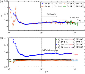
The total entrainment coefficient  $E$ is then obtained using (4.14) with the profile coefficients given in table 2. Results are shown in figure 13(a), where
 $E$ calculated from (4.14) is compared with that from (4.12), i.e.
 $E=v_e/ \hat {u}$. Evidently, from figure 13(a), the calculated
 $E$ shows good agreement between the two methods. Figure 13(b) demonstrates the development of the individual contributions, (4.15), to the entrainment coefficient against
 $\textit {Gr}_\delta$. It is evident that all the components tend to be constants beyond
 $\textit {Gr}_\delta =10^7$. The shear production term
 $E_p$, among all the components, is of the leading order. In the present study, we have found
 $E_p\approx 0.041$, which is approximately half of the values reported by previous studies for free shear flows: in an energy-consistent analysis, van Reeuwijk & Craske (Reference van Reeuwijk and Craske2015) reported that the shear production contribution is insensitive to the Richardson number, where
 $E_p \approx 0.08$, for the spatially developing axisymmetric jets (
 $\textit {Ri}=0$) and plumes (
 $0.1< Ri<0.2$). Krug et al. (Reference Krug, Chung, Philip and Marusic2017) numerically obtained
 $E_p\approx 0.08$ for a temporally developing planar plume at
 $\textit {Ri}=0.2$ and
 $E=E_p\approx 0.12$ for a temporally developing planar jet (
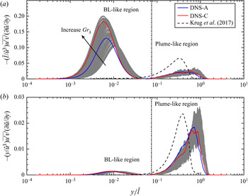
 $\textit {Ri}=0$) using DNS. This discrepancy is essentially due to the shear production profile difference between the free shear flows and the NCBL, as shown in figure 14. It is worth noting that the data presented in Krug et al. (Reference Krug, Chung, Philip and Marusic2017) was originally normalised by a centreline velocity of the plume
 $\bar {w}_{cl}$, where such centreline velocity is not applicable in the current NCBL flow. As such, we have assumed the mean profile of their plume data to be Gaussian, so that
 $\bar {w}_{cl}=\sqrt {2}\hat {u}$ is used to compare with our data in figure 14. As shown in figure 14(a), the NCBL develops two shear layers. The first peak of the shear production occurs in the near-wall region since the NCBL is bounded by the wall (see also in figure 6a, the maximum shear production occurs when
 $-\overline {u'v'} = \nu \partial \bar u /\partial y$). The near-wall peak, when scaled by the characteristic scales, increases with increase
 $\textit {Gr}_\delta$, whereas the second peak takes place in the plume-like region (
 $y>\delta _i$). In the plume-like region, our DNS data shows fairly good agreement between the relatively low
 $\textit {Gr}_\delta$ case (DNS-A) and high
 $\textit {Gr}_\delta$ case (DNS-C), convincingly showing that the statistics of the plume-like region are in the self-similar state. We stress that the near-wall shear production contributes minimally to the integral shear production term
 $E_p=-\gamma _p$ given the near-wall region is extremely thin, for example, the difference between integrating from
 $y=0$ and
 $y=\delta _i$ to
 $y=L_y$ at
 $\textit {Gr}_\delta =1.2\times 10^8$ is less than
 $5\,\%$. This is more clearly demonstrated in figure 14(b), where the shear production is premultiplied by the dimensionless wall-normal distance
 $y/\hat {l}$. Although different in shape, the contributions to the integral (area under the curve) for the present study roughly matches the temporal plume data reported by Krug et al. (Reference Krug, Chung, Philip and Marusic2017) in figure 14(b). Note in Krug et al. (Reference Krug, Chung, Philip and Marusic2017) the shear production contribution to the entrainment is defined by the integral in the cross-stream direction, i.e.
 $-\infty$ to
 $\infty$, whereas figure 14 only shows
 $0$ to
 $\infty$. As a result, the total shear production in the plume-like region is approximately half of the value reported by Krug et al. (Reference Krug, Chung, Philip and Marusic2017). More recently, Parker et al. (Reference Parker, Burridge, Partridge and Linden2020) compared the entrainment due to shear production between a spatially developing wall plume (
 $\textit {Ri}=0.09$) and a free planar plume (
 $\textit {Ri}=0.23$) and found the total shear production for the wall plume (
 $E_p=0.067$) is slightly higher than half of that for the free plume (
 $E_p=0.103$). The discrepancy between the NCBL flow reported here and the wall plume may be due to differences in the driving mechanisms and flow conditions. Nevertheless, both planar (temporal) and axisymmetric (spatial) flows suggest the entrainment process is dominated by the shear production (Craske & van Reeuwijk Reference Craske and van Reeuwijk2015; van Reeuwijk & Craske Reference van Reeuwijk and Craske2015; Krug et al. Reference Krug, Chung, Philip and Marusic2017), consistent with the current study.
Development of the entrainment coefficient. (a) The total entrainment coefficient  $E$ and (b) buoyancy
 $E_b$, shear
 $E_p$, BCs
 $E_s$ and viscous
 $E_\nu$ contributions to the entrainment coefficient
 $E$.

Dimensionless (a) shear production and (b) premultiplied shear production for the NCBL. Grey solid lines show the instantaneous shear production profiles for the turbulent NCBL from both DNS-A and DNS-C, in the range  $10^7<\textit {Gr}_\delta <1.2\times 10^8$; solid lines also show the ensemble average of the dimensionless shear production in DNS-A (blue, over the range
 $10^7<\textit {Gr}_\delta <7.7\times 10^7$) and DNS-C (red, over the range
 $5\times 10^7<\textit {Gr}_\delta <1.2\times 10^8$); black dashed line indicates the shear production profile take from Krug et al. (Reference Krug, Chung, Philip and Marusic2017) for a temporally evolving planar plume; vertical line indicates the starting point of the plume-like region (maximum velocity location)
 $y=\delta _i$.

The effect of buoyancy on the entrainment, given in (4.15a), can be rewritten in the form of
 \begin{equation} E_b = Ri(2-\gamma_b) = \frac{2}{\hat{u}^3}\left(\frac{\displaystyle\int^{\infty}_{\delta_i}{\bar{u}}^2\, \mathrm{d} y \int^{\infty}_{\delta_i}\bar b \,\mathrm{d} y}{\displaystyle\int^{\infty}_{\delta_i}\bar u \,\mathrm{d} y} - \int^{\infty}_{\delta_i} \bar u \bar b \,\mathrm{d} y\right), \end{equation}
where the first term in the bracket is associated with the rate of change in volume flux  $\partial Q/\partial t$ due to the total buoyancy and the second term in the bracket represents the rate of change in the momentum flux
 $\partial M / \partial t$ due to the mean buoyancy flux in the plume-like region. The whole term (4.16) can only become zero when the mean velocity and mean buoyancy (temperature) profiles share the same width and shape (see also Krug et al. Reference Krug, Chung, Philip and Marusic2017). This is consistent with the
 $\alpha$-MSG model derived by van Reeuwijk & Craske (Reference van Reeuwijk and Craske2015), where the spreading rate (
 $\partial \hat {l}/\partial z$) is found independent of
 $E_b$, as the velocity and buoyancy are assumed to take Gaussian profiles of equal width in the model. Parker et al. (Reference Parker, Burridge, Partridge and Linden2020) obtained the buoyancy effect
 $E_b\approx 0.043\text {--}0.047$ for both spatially developing free and wall plumes. Their measurements are consistent with the experimental measurements reported by Paillat & Kaminski (Reference Paillat and Kaminski2014)
 $E_b\approx 0.04$. For a temporally developing planar plume, Krug et al. (Reference Krug, Chung, Philip and Marusic2017) suggests the buoyancy effect contributes approximately
 $15\,\%$ to the total entrainment coefficient, which is
 $E_b \approx 0.015$, smaller than that reported by Parker et al. (Reference Parker, Burridge, Partridge and Linden2020). In their DNS study, they point out that a smaller
 $E_b$ is attained due to the fundamental difference between the spatial and temporal flows – in spatially developing flows, the buoyancy additionally affects the streamwise transport of the momentum and energy, causing a net-buoyancy contribution to the entrainment, whereas such modification is absent in the temporal flows (Krug et al. Reference Krug, Chung, Philip and Marusic2017). In the present study, we have found
 $E_b\approx -0.0022$ negatively contributing to the spreading of the flow, and is one order of magnitude smaller than the values reported in the aforementioned studies. Such a result does not imply our results contradict previous studies, for the buoyancy contribution
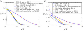
 $E_b$ fully depends on the shapes of the profiles of velocity and buoyancy of the flow as given in (4.16). Figure 15 compares the velocity and buoyancy profiles for the plume and NCBL. According to figure 15(a), the streamwise mean velocity profiles for the plumes from different sources (Ramaprian & Chandrasekhara Reference Ramaprian and Chandrasekhara1989; Paillat & Kaminski Reference Paillat and Kaminski2014; Krug et al. Reference Krug, Chung, Philip and Marusic2017; Parker et al. Reference Parker, Burridge, Partridge and Linden2020) collapse into a single curve, while the wall plume DNS data (Parker et al. Reference Parker, Burridge, Partridge and Linden2020) demonstrates a slight difference in the near-wall region (
 $y^*/\hat {l}<0.1$) due to the wall friction. Here, the corrected coordinate is given by
 \begin{equation} y^*=\begin{cases} y-\delta_i, & \text{for NCBL},\\ y, & \text{for plumes}. \end{cases} \end{equation}
The DNS data for the NCBL, however, exhibits a different shape in comparison with the plume velocity profiles. Similar behaviour can also be observed in figure 15(b), where the mean buoyancy profile of the NCBL is shown along with those of the plumes. The wall plume case (Parker et al. Reference Parker, Burridge, Partridge and Linden2020) again diverges from the free shear plumes up to  $y^*/\hat {l}=0.5$ due to the presence of the non-slip wall. It is clear that the plume buoyancy profiles given in figure 15(b) are quite different from the NCBL flow. A small buoyancy contribution (compared with
 $15\,\%$ in Krug et al. (Reference Krug, Chung, Philip and Marusic2017) and over
 $30\,\%$ in Parker et al. (Reference Parker, Burridge, Partridge and Linden2020)) is not surprising since the discrepancy in the profiles directly lead to a different buoyancy contribution to the entrainment. Assuming a self-similar mean flow, van Reeuwijk & Craske (Reference van Reeuwijk and Craske2015) showed the buoyancy effect can both positively and negatively contribute to the entrainment coefficient, with the net-effect depending on the profile coefficients, for spatial plumes. In the present temporally developing NCBL, the profile coefficient
 $\gamma _b \approx 2.045$ is always greater than
 $2$. According to (4.15a), this determines a negative net-effect on the entrainment coefficient.
Profile shape comparison of (a) mean streamwise velocity and (b) mean buoyancy. Filled markers represent experimental measurements for pure plumes, yellow circles, Paillat & Kaminski (Reference Paillat and Kaminski2014); blue triangles, Ramaprian & Chandrasekhara (Reference Ramaprian and Chandrasekhara1989). Lines represent DNS studies: red solid, planar plume reported by Krug et al. (Reference Krug, Chung, Philip and Marusic2017); blue solid and red dashed lines are the present study. Here  $y^*$ is a corrected coordinate, given by
 $y^* = y-\delta _i$ for the NCBL and
 $y^*=y$ for the plumes.

The viscous and BC contributions to the entrainment coefficient are found to be  $E_\nu \approx 2\times 10^{-4}$ and
 $E_s\approx -0.0037$, respectively, for the NCBL. With increasing
 $\textit {Gr}_\delta$, the viscous effect
 $E_\nu$ continues to lose its significance (see also in figure 11b,c); whereas the magnitude of
 $E_s$ appears independent of
 $\textit {Gr}_\delta$. By subtracting
 $E_b$ and
 $E_p$ from the spreading rate (
 $\partial \hat {l}/\partial z$), Parker et al. (Reference Parker, Burridge, Partridge and Linden2020) obtained a viscous component of
 $E_s^*\approx -0.03$ in their spatially developing wall plume. Note the viscous component
 $E_s^*$ in Parker et al. (Reference Parker, Burridge, Partridge and Linden2020) contains the combined effect of the BC
 $E_s$ and the viscous effect
 $E_\nu$ since it includes the wall shear and viscous dissipation. However, as noted by van Reeuwijk & Craske (Reference van Reeuwijk and Craske2015), the entrainment and the spreading rate of the spatially developing plumes are usually different – except in the case of fully self-similar Gaussian plumes.
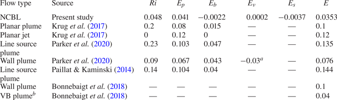
A brief comparison of the entrainment coefficient between the NCBL and previous studies is summarised in table 3. The current study suggests a constant entrainment coefficient of  $E\approx 0.0353$ for the turbulent NCBL, giving good agreement with the experimental measurement (
 $E=0.04$) obtained by Bonnebaigt, Caulfield & Linden (Reference Bonnebaigt, Caulfield and Linden2018) for a plume with vertically distributed buoyancy source. It is evident that the production of turbulent kinetic energy
 $E_p$ is mainly responsible for the spreading of the plume-like region in the NCBL, whereas buoyancy
 $E_b$, viscous
 $E_\nu$ and BCs
 $E_s$ have negligible effects.
Entrainment (spreading) coefficient components for the temporally developing NCBL, plume and jets. Supercripts:  $^{a}$ this is effectively
 $E_\nu +E_s$;
 $^{b}$ a plume with vertically distributed buoyancy source along the wall.

4.4. Solution to the self-similar system
As demonstrated in §§ 4.2 and 4.3, the outer plume-like region of the NCBL flow appears to be self-similar in the current  $\textit {Gr}_\delta$ range and can be fully described by the integral model given in (3.6). It is convenient to rewrite (3.6) here in terms of the local (instantaneous) top-hat characteristic scales in order to obtain the solutions to the flow system:
 \begin{gather} \frac{\partial }{\partial t} [\hat{u}\hat{l}] = \hat{b}\hat{l} - {\hat{u}^2}(S_{\delta_i}+\mathcal{L}_Q), \end{gather}
 \begin{gather}\frac{\partial }{\partial t} [\hat{b}\hat{l}] = {\hat{u}\hat{b}}(\beta_{\delta_i}-\mathcal{L}_B), \end{gather}
 \begin{gather}\frac{\partial }{\partial t} [\hat{u}^2\hat{l}]= \hat{u}^3(M_{\delta_i}+\gamma_p+\gamma_d+\gamma_f-\mathcal{L}_M)+ \hat{u}\hat{l}\hat{b}\gamma_b, \end{gather}
The dimensional consistency of (4.18) allows the following scaling relations for the characteristic scales in terms of total buoyancy  $B$ and time
 $t$ (see Appendix A for detailed derivation):
 \begin{align} \hat{u} = k_{\hat{u}}\sqrt{B}, \end{align}
 \begin{align} \hat{b} = k_{\hat{b}}\sqrt{B}/t, \end{align}
 \begin{align} \hat{l} = k_{\hat{l}}\sqrt{B}t, \end{align}
where  $k_{\hat {u}}$,
 $k_{\hat {b}}$ and
 $k_{\hat {l}}$ are constants based on the profile coefficients,
 \begin{gather} k_{\hat{u}} = \left[\frac{1-\gamma_b}{S_{\delta_i}+\mathcal{L}_Q+M_{\delta_i}+\gamma_p+\gamma_d+\gamma_f-(\beta_{\delta_i}-\mathcal{L}_B)/2}\right]^{1/2}, \end{gather}
 \begin{gather}k_{\hat{b}} = \frac{1}{k_{\hat{l}}}, \end{gather}
 \begin{gather}k_{\hat{l}} =\frac{1-k_{\hat{u}}^2(S_{\delta_i}+\mathcal{L}_Q+\beta_{\delta_i}-\mathcal{L}_B)} {k_{\hat{u}}}. \end{gather}
The scaling relations obtained here in (4.19) take a similar form to those suggested by Krug et al. (Reference Krug, Chung, Philip and Marusic2017) for the temporally developing planar plume. Note in Krug et al. (Reference Krug, Chung, Philip and Marusic2017),  $B$ is a constant independent of time since the buoyancy is conserved; whereas in our temporal NCBL buoyancy is accumulating due to the existence of heat flux from the isothermal wall and fully depends on the local characteristic scales, i.e.
 $B(t)=\hat {b}\hat {l}$.
Since the profile coefficients are found to be constant for the current range of  $\textit {Gr}_\delta$ (e.g. table 2), the set of ordinary differential equations (ODE) can be recast in the following form which encapsulates the entrainment assumption (4.12):
 \begin{gather} \frac{\partial \hat{u}}{\partial t} = \hat{b}-(E+S_{\delta_i}+\mathcal{L}_Q)\frac{\hat{u}^2}{\hat{l}}, \end{gather}
 \begin{gather}\frac{\partial \hat{b}}{\partial t} = (\beta_{\delta_i}-E-\mathcal{L}_B)\frac{\hat{u}\hat{b}}{\hat{l}}, \end{gather}
 \begin{gather}\frac{\partial \hat{l}}{\partial t} = E \hat{u}. \end{gather}
System (4.21) yields a power-law solution (see the more detailed derivation in Appendix A),
 \begin{gather} \hat{u} = A_{\hat{u}} t^{\xi} = k_{\hat{u}}A_{\hat{b}}^{1/2}A_{\hat{l}}^{1/2} t^{\xi}, \end{gather}
 \begin{gather}\hat{b} = A_{\hat{b}} t^{\xi-1 }, \end{gather}
 \begin{gather}\hat{l} = A_{\hat{l}} t^{ \xi+1 }, \end{gather}
where the exponent  $\xi$ is given by
 \begin{equation} \xi = \frac{\beta_{\delta_i}-\mathcal{L}_B}{2E-\beta_{\delta_i}+\mathcal{L}_B}, \end{equation}
and  $A_{\hat {b}}$ and
 $A_{\hat {l}}$ are constants from the integration which can be determined by the initial conditions. In the present study, the power-law solutions (4.22) are obtained using the constant profile coefficients in table 2 and the initial conditions
 $\hat {u}= 30.42$,
 $\hat {b}=0.1278$ and
 $\hat {l}=350.5$ from DNS-A at
 $\textit {Gr}_\delta =3.75\times 10^7$. The resultant integral constants and exponents for the power-law solution are tabulated in table 4. Note the initial condition is chosen arbitrarily from the DNS data, a different choice of the initial condition would result in a slightly different value for
 $A_b$ and
 $A_l$ due to the temporal nature of our DNS (for instance, at
 $\textit {Gr}_\delta =2.11\times 10^7$ gives
 $A_b=1.375$ and
 $A_l=0.0163$). Figure 16 compares the characteristic scales for the plume-like region predicted by the power-law solution (4.22) and the numerically generated data by DNS. The Grashof number is estimated by the characteristic length scale,
 \begin{equation} \textit{Gr}_\delta \equiv \frac{g\alpha \theta_w\delta^3}{\nu^2} = \frac{g\alpha \theta_w\hat{l}^3}{\nu^2} \frac{1}{\lambda_\delta^3}, \end{equation}
where  $\lambda _\delta$ is the ratio of the characteristic length scale
 $\hat {l}$ to the velocity integral boundary layer thickness
 $\delta$. In the present study, it has been found that
 \begin{equation} \lambda_\delta \equiv \frac{\hat{l}}{\delta} \approx 1.33, \end{equation}
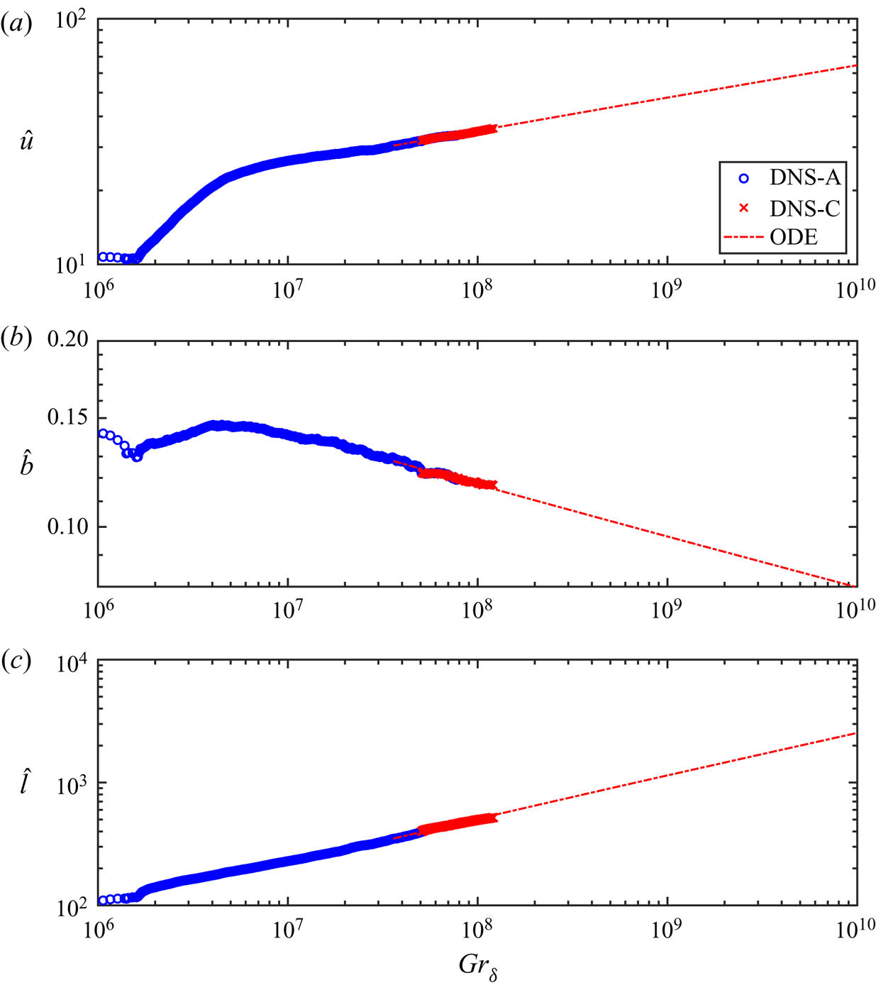
is a constant in the self-similar regime ( $\textit {Gr}_\delta >10^7$). Shown by figure 16, the characteristic scales predicted by the ODE system exhibit excellent agreement with the DNS data, indicating the plume-like region can be well described by the self-similar model (4.21) using constant profile coefficients given in table 2.

Development of the top-hat characteristic scales for the plume-like region of the NCBL against  $\textit {Gr}_\delta$: (a) the characteristic velocity scale
 $\hat {u}$; (b) the characteristic buoyancy scale
 $\hat {b}$; (c) the characteristic length scale
 $\hat {l}$.

4.5. Wall heat transfer characteristics
With the ODE system given in (4.21), it is also possible to predict the evolution of the wall heat flux with the growth of the boundary layer thickness for the turbulent NCBL. The wall heat transfer is typically characterised by the Nusselt number, which is defined as
 \begin{equation} \textit{Nu}_\delta \equiv \frac{\delta q_w}{\kappa \theta_w}. \end{equation}
Since the wall heat flux  $q_w$ is directly linked to the BC for the integral model as given in (4.8), the Nusselt number in (4.26) can be written in terms of the local (instantaneous) top-hat characteristic scales,
 \begin{equation} \textit{Nu}_\delta = \frac{\beta_{\delta_i}}{ g\alpha \kappa \theta_w \lambda_\delta} \hat{u}\hat{b}\hat{l} \propto \hat{u}\hat{b}\hat{l}. \end{equation}
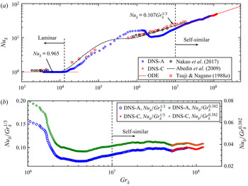
Figure 17(a) compares the  $\textit {Nu}_\delta$ result of the present DNS study with the ODE prediction (4.27) and previous studies. For the spatially developing NCBL (Tsuji & Nagano Reference Tsuji and Nagano1988; Nakao et al. Reference Nakao, Hattori and Suto2017), the flow undergoes turbulent transition at
 $\textit {Gr}_\delta =10^6$, and the Nusselt number then has the empirical correlation,
 \begin{equation} \textit{Nu}_\delta = 0.107\textit{Gr}_\delta^{1/3}, \end{equation}
in the turbulent regime. Abedin et al. (Reference Abedin, Tsuji and Hattori2009) showed that their DNS data for a temporally developing NCBL closely follows the empirical correlation for the spatial flows. However, the temporally developing NCBL in the present study is not yet turbulent at  $\textit {Gr}_\delta =10^6$. The discrepancy may be due to the fact that statistics in Abedin et al. (Reference Abedin, Tsuji and Hattori2009) are obtained by taking ensemble average of multiple simulations with different initialisation. At
 $\textit {Gr}_\delta =10^7$, our temporally developing NCBL becomes turbulent and the plume-like region appears self-similar. As shown in figure 17(a), our DNS data follow a similar trend to (4.28) in the turbulent regime. However, the power-law regression of our DNS data at
 $\textit {Gr}_\delta >10^7$ yields a slightly higher exponent than
 $1/3$, giving
 \begin{gather} \textit{Nu}_\delta=0.0512\textit{Gr}_\delta^{0.369},\quad \text{for DNS-A}, \end{gather}
 \begin{gather}\textit{Nu}_\delta=0.0399\textit{Gr}_\delta^{0.382},\quad \text{for DNS-C}, \end{gather}
with  $95\,\%$ confidence bounds. The difference between the power-law scalings (4.28) and (4.29b) is rather subtle in the current DNS range, as shown in figure 17(b). In addition, the turbulence shows up in the Nusselt number due to the temporal nature of our NCBL, making the detection of an accurate power-law scaling difficult in the current
 $\textit {Gr}_\delta$ range. We, therefore, seek a different approach to accurately determine the scaling exponent for the Nusselt number in the current Grashof number range.
Nusselt number development for the temporally developing NCBL: (a) comparing with the data reported by Tsuji & Nagano (Reference Tsuji and Nagano1988) and Nakao et al. (Reference Nakao, Hattori and Suto2017) for spatially developing NCBLs and Abedin et al. (Reference Abedin, Tsuji and Hattori2009) for a temporally developing NCBL; (b) compensated Nusselt number development for the temporally developing NCBL in the self-similar turbulent region.

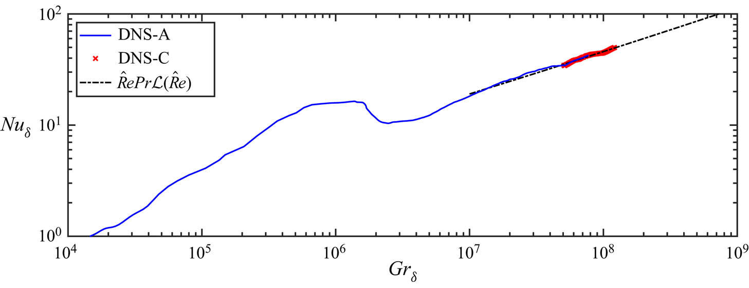
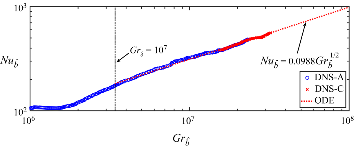
The  $\textit {Nu}_\delta$ predictions made from the ODE based, power-law solution (4.27), show excellent agreement with the data from both DNS-A and DNS-C, indicating the wall heat flux is indeed controlled by the characteristic scales from the plume-like region. Given by the power-law solution, (4.22), and making use of (4.24) and (4.27), the Nusselt number follows
 \begin{equation} \textit{Nu}_\delta \propto \textit{Gr}_\delta^{ 3\xi/(3\xi+3)}\approx 0.0408\textit{Gr}_\delta^{0.381}. \end{equation}
This  $0.381$-power-law relation is consistent with the ultimate heat transfer scaling with a logarithmic correction reported by Ng et al. (Reference Ng, Ooi, Lohse and Chung2017), who obtained an empirical correlation
 \begin{equation} \textit{Nu}_\delta \propto \textit{Gr}_\delta^{0.37}, \end{equation}
after conditionally averaging the high wall shear events in their DNS study of an NCBL in a differentially heated vertical slot. Ng et al. (Reference Ng, Ooi, Lohse and Chung2017) suggest that the slightly higher  $\textit {Nu}_\delta$–
 $\textit {Gr}_\delta$ power-law correlation in (4.31) is consistent with the ultimate turbulent regime power-law scaling with a logarithmic correlation. The exponent is also close to an experimental study by He et al. (Reference He, Funfschilling, Nobach, Bodenschatz and Ahlers2012), who gives 0.38, for Rayleigh–Bénard convection at high Rayleigh number. A higher exponent has been reported by Eckert & Jackson (Reference Eckert and Jackson1950) – although the mean profiles were modelled by a
 $1/7$-power-law, they showed that the Nusselt number would follow
 $\textit {Nu}_\delta \propto \textit {Gr}_\delta ^{0.429}$ if the boundary layer is turbulent in the sense of Prandtl and von Kármán (i.e. momentum-dominated boundary layers).
4.6. Logarithmic correction for the ultimate turbulent regime
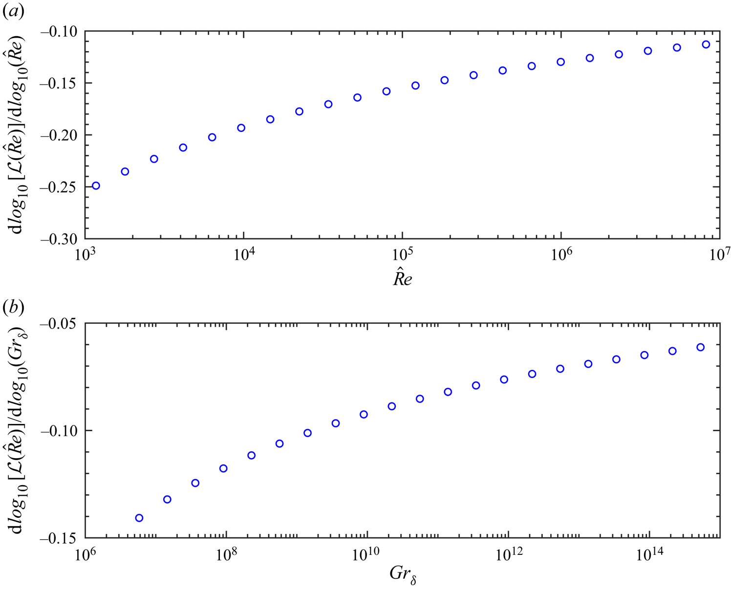
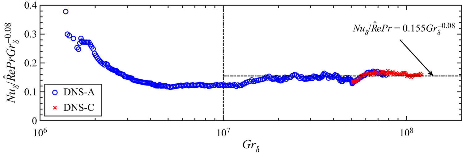
The Nusselt number correlation given by (4.30) suggests that the heat transfer of the temporally developing NCBL is driven by the bulk thermal convection in the plume-like region and limited by near-wall processes as seen in Rayleigh–Bénard convection. In the so-called ultimate turbulent regime, the boundary layer is dominated by the bulk thermal convection in the sense of Grossmann & Lohse (Reference Grossmann and Lohse2000, Reference Grossmann and Lohse2011), and the  $\textit {Nu}_\delta$ follows
 \begin{equation} \textit{Nu}_\delta \propto \textit{Re} \mathcal{L}(\textit{Re}), \end{equation}
as in homogeneous Rayleigh–Bénard convection, where  $\textit {Re}$ is the bulk Reynolds number, and
 $\mathcal {L}(\textit {Re})$, being a function of Reynolds number, is a logarithmic-correction term for the turbulent kinetic boundary layer. The Reynolds number
 $\textit {Re}$ is then related to the Rayleigh number
 $\textit {Ra}$, giving
 $\textit {Re}\propto \textit {Ra}^{1/2}$ in the ultimate turbulent regime, for their Rayleigh–Bénard convection. It is noted in the vertical NCBL flow the gravity vector is perpendicular to the driving heat flux, whereas in the Rayleigh–Bénard convection the gravity is aligned with the driving heat flux. In our previous study (Ke et al. Reference Ke, Williamson, Armfield, Norris and Komiya2020), we have shown that the mean profiles follow a buoyancy-modified law of the wall for the NCBL (see also in figure 7). Following Grossmann & Lohse (Reference Grossmann and Lohse2011), the temperature log-law can be rewritten into
 \begin{equation} \frac{\theta_\tau}{\theta_w - \theta_{log}} = \frac{K_\theta}{\ln\left(\hat{\textit{Re}}\dfrac{u_\tau}{\hat{u}}e^{B_\theta K_\theta}\right)}, \end{equation}
where  $\theta _{log}$ denotes the temperature at the end of the log-law region,
 $K_\theta$ is the thermal von Kármán constant, given by the ratio of von Kármán constant
 $K_v$ to the turbulent Prandtl number
 $\textit {Pr}_t$,
 $B_\theta$ is the constant from the temperature log-law, and the bulk Reynolds number
 $\hat {\textit {Re}}$ is given by the velocity scale in the plume-like region
 $\hat {u}$ and the length of the log-law
 $l_m$, as follows:
 \begin{equation} \hat{\textit{Re}} \equiv \frac{\hat{u}l_m}{\nu}. \end{equation}
In the present study, we assume the log-law extends up to the maximum velocity location (see also in Ke et al. (Reference Ke, Williamson, Armfield, Norris and Komiya2020)), i.e.  $l_m\approx \delta _i$. Making a substitution of (4.6) and (4.33) into the Nusselt number definition, (4.26), yields
 \begin{equation} \textit{Nu}_\delta=\frac{\hat{\textit{Re}}\textit{Pr}\dfrac{u_\tau}{\bar{u}_m}\dfrac{\bar{u}_m}{\hat{u}}K_\theta} {\ln\left(\hat{\textit{Re}}\dfrac{u_\tau}{\bar{u}_m}\dfrac{\bar{u}_m}{\hat{u}}\,\textrm{e}^{B_\theta K_\theta}\right)}\frac{\delta}{\delta_i} \frac{(\theta_w-\theta_{log})}{(\theta_w-\theta_\infty)}. \end{equation}
For asymptotically high  $\textit {Gr}_\delta$ NCBL flows, the near-wall buoyancy effect would become negligible and the velocity is expected to follow a similar log-law to the momentum dominated flows (Ke et al. Reference Ke, Williamson, Armfield, Norris and Komiya2020), in the form of
 \begin{equation} \frac{u_\tau}{\bar{u}_m} = \frac{K_v}{\ln\left(\hat{\textit{Re}}\dfrac{u_\tau}{\bar{u}_m}\dfrac{\bar{u}_m}{\hat{u}}e^{B_u K_v}\right)}, \end{equation}
where  $B_u$ is a constant for the velocity log-law. The Nusselt number scaling (4.35) can be further simplified into
 \begin{equation} \textit{Nu}_\delta=\hat{\textit{Re}}\textit{Pr} \mathcal{L}(\hat{\textit{Re}}), \end{equation}
which takes the same form as (4.32) given by Grossmann & Lohse (Reference Grossmann and Lohse2011), with the logarithmic correction term
 \begin{equation} \mathcal{L}(\hat{\textit{Re}}) = \frac{\mathcal{B}}{\ln\left(\hat{\textit{Re}}\dfrac{u_\tau}{\bar{u}_m}C_u\right) \ln\left(\hat{\textit{Re}}\dfrac{u_\tau}{\bar{u}_m}C_\theta\right)}, \end{equation}
and the coefficients  $\mathcal {B}$,
 $C_u$ and
 $C_\theta$ are given by
 \begin{equation} \mathcal{B} =K_v K_\theta \frac{\delta \bar{u}_m(\theta_w-\theta_{log})}{\delta_i \hat{u}(\theta_w-\theta_\infty)}, \quad C_u = \frac{\bar{u}_m}{\hat{u}} e^{K_v B_u}, \quad C_\theta = \frac{\bar{u}_m}{\hat{u}}e^{B_\theta K_\theta}. \end{equation}
Equation (4.37) indicates that  $\textit {Nu}_\delta$ scales with the bulk Reynolds number
 $\hat {\textit {Re}}$ in the plume-like region with the logarithmic correction (4.38).
The logarithmic correction term (4.38), however, depends on the bulk Reynolds number  $\hat {\textit {Re}}$, the velocity ratio
 ${u_\tau }/{\bar {u}_m}$ and the coefficients
 $\mathcal {B}$,
 $C_u$ and
 $C_\theta$. The velocity ratio
 ${u_\tau }/{\bar {u}_m}$ is implicitly given by the continuous fraction (4.36) and has analytical solution (Grossmann & Lohse Reference Grossmann and Lohse2011)
 \begin{equation} \frac{u_\tau}{\bar{u}_m} = \frac{K_v}{\omega(\hat{\textit{Re}}K_v C_u)}, \end{equation}
where  $\omega (\phi )$ denotes the Wright omega function of
 $\phi$. In the present study, the bulk velocity and length scales are found to scale with the characteristic scales for the plume-like region, i.e.
 $\bar {u}_m/\hat {u}\approx 1.475$ and
 $\delta _i/ \delta \approx 0.1035$ are approximately constant in the current
 $\textit {Gr}_\delta$ range, as shown in figure 18(a,b). The
 $\delta _i/\delta$ value reported here is also close to the measurement of Tsuji & Nagano (Reference Tsuji and Nagano1988) and Abedin et al. (Reference Abedin, Tsuji and Hattori2009) at lower Grashof number range, which is
 $\delta _i/\delta = 0.07$. The temperature ratio
 $(\theta _w-\theta _{\textit {log}})/(\theta _w-\theta _\infty )$, on the other hand, is thought to be varying slowly since the temperature difference across the logarithmic region would increase slowly with
 $\textit {Gr}_{\delta }$ (we emphasise the very large
 $\textit {Gr}_{\delta }$ range here). As shown in figure 18(c), the temperature ratio
 $(\theta _w-\theta _{\textit {log}})/(\theta _w-\theta _\infty )$ demonstrates weak
 $\textit {Gr}_{\delta }$-dependency in the current
 $\textit {Gr}_{\delta }$ range, therefore, it appears reasonable to assume a constant temperature ratio in our
 $\textit {Gr}_{\delta }$ range. This suggests that
 $\mathcal {B}$,
 $C_\theta$ and
 $C_u$ are all approximately constant. With substitution of (4.40) into (4.38), the logarithmic correction term depends solely on the bulk Reynolds number
 $\hat {\textit {Re}}$. Unfortunately, the
 $\hat {\textit {Re}}$-dependency of (4.38) is difficult to obtain analytically. However, since
 $K_v$,
 $K_\theta$ and the bulk scale ratios (
 $\bar {u}_m/\hat {u}$ and
 $\delta /\delta _i$) are all approximately constants in the current Grashof number range Grashof number range (values tabulated in table 5), we are able to calculate (4.38) numerically. The local effective scaling exponent
 $\mathrm {d} \log \mathcal {L}(\hat {\textit {Re}})/\mathrm {d} \log \hat {\textit {Re}}$, as shown in figure 19(a), is found to be varying slowly with
 $\hat {\textit {Re}}$. The gradually reducing magnitude of the effective scaling exponent indicates the
 $\hat {\textit {Re}}$-dependency becomes weaker with increasing
 $\hat {\textit {Re}}$. We stress that (4.36) and (4.40) are approximations for asymptotically high
 $\textit {Gr}_{\delta }$ flow since the buoyancy effect (which will vary with
 $\textit {Gr}_{\delta }$ and
 $\hat {\textit {Re}}$) is not accounted for (Ke et al. Reference Ke, Williamson, Armfield, Norris and Komiya2020), and only at this asymptotic
 $\textit {Gr}_{\delta }$ range will these relations hold. Nevertheless, we present figure 19(a), based on the asymptotic relations (4.36) and (4.40), for illustrative purposes, as the general behaviour of the logarithmic correction term is the same.
Temporal development of the scale ratios: (a)  $\bar {u}_m/\hat {u}$; (b)
 $\delta _i/\delta$; (c)
 $(\theta _w-\theta _{\textit {log}})/(\theta _w-\theta _\infty )$. Horizontal black dash–dotted lines indicates the temporal average:
 $\bar {u}_m/\hat {u}=1.475$;
 $\delta _i/\delta =0.1035$;
 $(\theta _w-\theta _{\textit {log}})/(\theta _w-\theta _\infty )=0.735$.

Making use of (4.25) and  $\delta _i\propto \delta$ in the current range of Grashof number, the bulk Reynolds number then scales with the ODE solution,
 \begin{equation} \hat{\textit{Re}} \propto \hat{u}\hat{l} \propto \textit{Gr}_{\delta}^{(2\xi+1)/(3\xi+3)}. \end{equation}
Based on the values tabulated in table 4, (4.41) is equivalent to a  $\hat {\textit {Re}}\approx 0.39 \textit {Gr}_{\delta }^{0.46}$ scaling for the current Grashof number range, close to the
 $\hat {\textit {Re}}\propto \textit {Gr}_{\delta }^{1/2}$ as suggested by Grossmann & Lohse (Reference Grossmann and Lohse2011) for Rayleigh–Bénard flow. With (4.41), it is also possible to obtain the development of a local effective scaling exponent in terms of Grashof number (
 $\mathrm {d} \log \mathcal {L}(\hat {\textit {Re}})/\mathrm {d} \log \textit {Gr}_\delta$), as shown in figure 19(b). Again we note that the mean velocity profile in the NCBL at non-asymptotic Grashof number is adjusted by buoyancy and takes a more complicated log-law (cf. Ke et al. (Reference Ke, Williamson, Armfield, Norris and Komiya2020), the extra buoyancy terms) than (4.36), resulting in a buoyancy-modified logarithmic correction term.
In the present study, the local effective scaling exponent for the logarithmic correction term is obtained empirically by
 \begin{equation} \mathcal{L}(\hat{\textit{Re}}) = \frac{\textit{Nu}_\delta}{\hat{\textit{Re}}\textit{Pr}}, \end{equation}
using DNS data. As shown in figure 20, for the current  $\textit {Gr}_{\delta }$ range the scaling exponent is found to be
 $-0.08$. In addition, the dimensional consistency between (4.30) and (4.37) further suggests
 \begin{equation} \mathcal{L}(\hat{\textit{Re}}) \propto \frac{\textit{Gr}_{\delta}^{3\xi/(3\xi+3)}}{\textit{Gr}_{\delta}^{(2\xi+1)/(3\xi+3)}} = \textit{Gr}_{\delta}^{(\xi-1)/(3\xi+3)}. \end{equation}
For the current range of  $\textit {Gr}_{\delta }$,
 $\xi =0.6156$ and the scaling exponent is found to be
 $-0.079$, consistent with the empirical results shown in figure 20. This indicates the Nusselt number is given by
 \begin{equation} \textit{Nu}_\delta\propto \hat{\textit{Re}}\textit{Pr} \mathcal{L}(\hat{\textit{Re}}) \propto \textit{Gr}_\delta^{0.46} \textit{Gr}_\delta^{{-}0.08} \approx \textit{Gr}_\delta^{0.38}. \end{equation}
This effective  $\textit {Nu}_\delta$–
 $\textit {Gr}_\delta$ scaling exponent, higher than the empirical
 $1/3$-power-law, is consistent with our
 $0.381$-power-law from the ODE prediction and DNS regression results in the current Grashof number range.
Constants for the mean velocity and temperature log-law.

The temporal development of the local effective scaling exponent for the logarithmic correction term; panel (b) shows same information as panel (a) but with Grashof number. The Grashof number  $\textit {Gr}_\delta$ is obtained by (4.41).

The compensated logarithmic correction scaling.

However, as depicted by figure 19, over a large range of  $\textit {Gr}_\delta$ the logarithmic correction
 $\mathcal {L}(\hat {\textit {Re}})$ is expected to vary very slowly with
 $\textit {Gr}_{\delta }$ (or
 $\hat {\textit {Re}}$), and would eventually approach to some constant at asymptotically high
 $\textit {Gr}_{\delta }$. This further implies that the exponent
 $\xi$ and, therefore, the profile coefficients and entrainment coefficient
 $E$ for the integral model, are also slowly varying quantities with
 $\textit {Gr}_{\delta }$ – again we emphasise the very large
 $\textit {Gr}_{\delta }$ range here. At asymptotically high
 $\textit {Gr}_{\delta }$,
 $\xi$ approaches to unity since (4.43) would become independent of Grashof number, and the Nusselt number would follow
 \begin{equation} \textit{Nu}_\delta\propto \hat{\textit{Re}}\textit{Pr} \mathcal{L}(\hat{\textit{Re}}) = \textit{Gr}_{\delta}^{1/2} \textit{Gr}_{\delta}^0 = \textit{Gr}_{\delta}^{1/2}, \end{equation}
consistent with the  $1/2$-power-law proposed by Wells & Worster (Reference Wells and Worster2008) and Grossmann & Lohse (Reference Grossmann and Lohse2011) for asymptotically high Grashof number. We stress that, similar to the logarithmic correction term, all the coefficients are very slowly varying, and can be approximately taken as constants for the current Grashof number range (
 $10^7<\textit {Gr}_\delta <1.2\times 10^8$). Nevertheless, making use of the values given in table 5, we are able to predict the Nusselt number based on (4.37). As demonstrated by figure 21, (4.37) still shows good agreement with the DNS data.
Nusselt number prediction using the logarithmic correction scaling (4.37).

This idea is further justified by identifying the local heat transfer in the plume-like part of the flow separately from the logarithmic region. The heat transfer within the plume-like region can be expressed in terms of a local Nusselt number and a local Grashof number,
 $$\begin{gather} \textit{Nu}_{\hat{b}} \equiv \frac{q_{\delta_i} \hat{l}}{\kappa\hat{b}}\approx\frac{q_{w} \hat{l}}{\kappa\hat{b}}\propto \frac{\hat{u}\hat{l}}{\kappa}, \quad \textit{Gr}_{\hat{b}} \equiv \frac{ \hat{b}\hat{l}^3}{\nu^2}. \end{gather}$$
With the ODE power-law solution (4.22), it immediately follows that
 \begin{equation} \textit{Nu}_{\hat{b}} \propto \textit{Gr}_{\hat{b}}^{(2\xi+1)/(4\xi+2)} =\textit{Gr}_{\hat{b}}^{1/2}. \end{equation}
This  $1/2$-power-law scaling is confirmed by our DNS data, as shown in figure 22, where the heat transfer into the plume-like region clearly demonstrates the scaling given in (4.47) since the near-wall logarithmic correction is absent in this region, indicating the plume-like region is dominated by the turbulent mixing in the sense of Grossmann & Lohse (Reference Grossmann and Lohse2000, Reference Grossmann and Lohse2001).
The local Nusselt number development in the plume-like region.

In the limit of asymptotically high Grashof number, (4.45) suggests that the Nusselt number would follow  $\textit {Nu}_\delta \propto \textit {Gr}_{\delta }^{1/2}$ since the logarithmic region is so large and the temperature across this logarithmic region increases at an asymptotically small rate. Similar results have been conjectured by Wells & Worster (Reference Wells and Worster2008), who used empirical correlations for the forced convection, suggesting at very high Grashof number the wall shear stress and heat flux follows
 \begin{gather} \tau_w = K_f\hat{u}^2, \end{gather}
 \begin{gather}q_w=\textit{St} \hat{u}\Delta T_{BL}, \end{gather}
where  $\Delta T_{BL} = T_{w}-\hat {b}/g\alpha$ is the near-wall temperature difference between the isothermal wall and the plume-like region,
 $K_f$ is the skin friction coefficient,
 $\textit {St}$ is the Stanton number. Based on the experimental measurements of Tsuji & Nagano (Reference Tsuji and Nagano1988), Wells & Worster (Reference Wells and Worster2008) suggest
 $K_f=0.0046$ and
 $\textit {St} = 0.0035$ are both constants. The Reynolds analogy allows (4.48) to be rewritten into
 \begin{equation} \frac{q_w}{(T_{w}-\hat{b}/g\alpha)\hat{u}} \propto \frac{\textit{Nu}_\delta}{\textit{Re}_{\delta}\textit{Pr}} \propto 2K_f, \end{equation}
where the Reynolds number is given by
 \begin{equation} \textit{Re}_{\delta} \equiv \frac{\hat{u}\delta}{\nu}. \end{equation}
Reynolds analogy has also been adopted by Eckert & Jackson (Reference Eckert and Jackson1950), where they assumed the NCBL shares a similar near-wall shear and heat transfer characteristics to those of a forced convection boundary layer, resulting a  $0.429$-power-law scaling for the Nusselt number. Rearranging (4.49) yields
 \begin{equation} \textit{Nu}_\delta \propto 2K_f \frac{\delta}{l_m} \hat{\textit{Re}}\textit{Pr}. \end{equation}
Equation (4.51) is, in general, consistent with the ultimate heat transfer correlation (4.37) suggested by Grossmann & Lohse (Reference Grossmann and Lohse2000, Reference Grossmann and Lohse2001, Reference Grossmann and Lohse2011): for a hydraulically smooth surface,  $K_f$ is usually a function of
 $\textit {Re}_{\delta }$ (cf. Eckert & Jackson Reference Eckert and Jackson1950), i.e.
 $K_f(\textit {Re}_{\delta })$; while a constant
 $K_f$, as suggested by Wells & Worster (Reference Wells and Worster2008), would indicate a hydraulically rough surface.
4.7. Wall shear stress characteristics
Unlike the Nusselt number, the wall shear stress  $\tau _w$ is not directly linked to the characteristic scales for the self-similar model. Given by (4.4), the wall shear stress is driven by the shear exerted by the plume-like region
 $\tau _{\delta _i}$ and the total buoyancy supplied by the isothermal wall in the near-wall region
 $B_i$ (see also in figure 6b),
 \begin{equation} \tau_w = \tau_{\delta_i} + B_i, \end{equation}
where the near-wall total buoyancy  $B_i$ is given by
 \begin{equation} B_i \equiv \int^{\delta_i}_0 \bar{b}\,\mathrm{d} y. \end{equation}
In the present study, the shear stress on the BL–plume interface is found to scale with the characteristic scales in the plume-like region,
 \begin{equation} \tau_{\delta_i} = S_{\delta_i}\hat{u}^2, \end{equation}
with the profile coefficient  $S_{\delta _i}$ being approximately a constant in the current Grashof number range. The near-wall buoyancy, however, can be expressed by
 \begin{equation} B_i = B_t - B, \end{equation}
where  $B$ is the total buoyancy within the plume-like region, as given in (3.3), and
 $B_t$ is the total buoyancy for the entire flow, i.e.
 \begin{equation} B_t \equiv \int^{\infty}_0 \bar{b} \,\mathrm{d} y. \end{equation}
Although (4.55) and (4.56) are not directly linked to the characteristic scales, the total buoyancy of the flow accumulates with time due to the wall heat flux,
 \begin{equation} \frac{\partial B_t}{\partial t} = q_w. \end{equation}
Since the BL–plume interface lies in the constant heat flux region, with (4.7), (4.57) can be simplified into
 \begin{equation} \frac{\partial B_t}{\partial t} =q_w\approx q_{\delta_i} =\beta_{\delta_i}\hat{u}\hat{b}. \end{equation}
The temporal evolution of the near-wall buoyancy is, therefore, given by
 \begin{equation} \frac{\partial B_i}{\partial t}=\frac{\partial (B_t - B)}{\partial t}=\frac{\partial B_t}{\partial t}-\frac{\partial B}{\partial t} = \mathcal{L}_B \hat{u}\hat{b}. \end{equation}
Here the Leibniz term  $\mathcal {L}_B$ also appears constant in the current Grashof number range (see table 2). As shown in (4.22), the dimensional consistency of the integral model also suggests that
 \begin{equation} \hat{u} =A_{\hat{u}} t^\xi,\quad \hat{b}= A_{\hat{b}} t^{\xi-1}. \end{equation}
Equation (4.59) can be integrated into
 \begin{equation} B_i =\frac{\mathcal{L}_BA_{\hat{u}}A_{\hat{b}}}{2\xi} t^{2\xi} + C_B = K_B \hat{u}^2+C_B, \end{equation}
where  $K_B = \mathcal {L}_BA_{\hat {b}}/(2\xi A_{\hat {u}})$ is a proportionality coefficient and
 $C_B$ is an integral constant.Figure 23 demonstrates the temporal development of the near-wall buoyancy
 $B_i$ using DNS data and a prediction made from (4.61) based on the constant coefficients given in tables 2 and 4. The integral constant is empirically found to be
 $C_B=5.5$ by fitting (4.61) to the DNS data.
The temporal development of the total buoyancy in the near-wall BL-like region  $B_i$.

The compensated wall shear stress scaling (4.62).

Equations (4.52), (4.54) and (4.61) indicate that the wall shear stress of the NCBL follows
 \begin{equation} \tau_w - C_B = (S_{\delta_i}+K_B)\hat{u}^2, \end{equation}
as shown in figure 24. At asymptotically high Grashof number (or, Reynolds number), the wall shear stress becomes large and
 \begin{equation} \tau_w-C_B \approx \tau_w. \end{equation}
This suggests that the wall shear stress, at asymptotically high Grashof number, scales with the bulk velocity scale
 \begin{equation} \tau_w \approx (S_{\delta_i}+K_B)\hat{u}^2, \end{equation}
as in the momentum-dominated flows.
5. Conclusions
In this paper, three-dimensional DNS are performed to investigate a turbulent temporally evolving NCBL along an isothermally heated vertical wall. To achieve a higher  $\textit {Gr}_\delta$ with minimal computational effort, we have initialised case DNS-C using turbulent flow fields of DNS-A at
 $\textit {Gr}_\delta =5\times 10^7$ and interpolated this data onto a larger domain and finer grid. The excellent agreement in DNS data between case DNS-A and DNS-C indicates initialising the flow using interpolated copies of turbulent flow fields in conjunction with the use of periodic BCs is adequate.
We examine the NCBL flow in two distinct regions separately – a BL-like region buried within the constant heat flux layer, and a plume-like region where the flow is dominated by the turbulent transport. The start of the plume-like region  $\delta _i$ is taken as the maximum mean streamwise velocity location for the results presented. However, we have also shown that the self-similar model is robust and insensitive to the choice of
 $\delta _i$ in the constant heat flux (forcing) layer. A modified integral model, retaining the BCs from the BL-like region and the viscous effects, is proposed to model the plume-like region of the NCBL at an integral level. Using DNS data, we have found that the plume-like region of the NCBL can be well approximated by the integral model and appears self-similar up to the limit of our data at
 $\textit {Gr}_\delta = 1.2\times 10^8$. In this self-similar turbulent regime, the Richardson number is also found to be a constant
 $\textit {Ri}=0.048$. The entrainment (expansion) coefficient
 $E$ of the plume-like region is obtained as
 $E\approx 0.0353$ for the self-similar turbulent regime, similar to the value reported by Bonnebaigt et al. (Reference Bonnebaigt, Caulfield and Linden2018) for a plume with vertically distributed buoyancy source. It is shown that the entrainment (expansion) coefficient
 $E$ is dominated by the shear production
 $E_p$ while the viscous
 $E_\nu$, buoyancy
 $E_b$ and BCs
 $E_s$ have minimal contribution to the entrainment coefficient for the NCBL.
The power-law solutions to the self-similar integral model ( $\hat {u}$,
 $\hat {b}$ and
 $\hat {l}$) are obtained by analytically solving the ODE with the profile constants. The ODE power-law solution shows excellent agreement with the existing DNS data up to
 $\textit {Gr}_\delta =1.21\times 10^8$. In the present study, we have also found the wall heat flux is directly linked to the buoyancy BC for the plume-like region (
 $q_w=q_{\delta _i}$) so that the Nusselt number
 $\textit {Nu}_\delta$ is determined by the characteristic scales which characterise the plume-like region. Based on the ODE solution, the Nusselt number is found to follow a
 $0.381$-power-law correlation with the Grashof number, similar to the observations in the high shear regions of the NCBL in a differentially heated vertical slot reported by Ng et al. (Reference Ng, Ooi, Lohse and Chung2017). The
 $0.381$-power-law scaling is also consistent with the ultimate heat transfer scaling in the sense of Grossmann & Lohse (Reference Grossmann and Lohse2011) – we show that the Nusselt number scales with the bulk Reynolds number
 $\hat {\textit {Re}}$ with a near-wall logarithmic correction
 $\mathcal {L}(\hat {\textit {Re}})$ due to the turbulent kinetic boundary layer. Using DNS data and law of the wall for the NCBL, the bulk Reynolds number is found to scale with
 $\textit {Gr}_{\delta }^{0.46}$ in the current Grashof number range, close to the
 $1/2$-power-law correlation in Rayleigh–Bénard convection (Grossmann & Lohse Reference Grossmann and Lohse2011); and the logarithmic correction
 $\mathcal {L}(\hat {\textit {Re}})$ is shown to have weak dependence on
 $\textit {Gr}_{\delta }$ – the local scaling exponent is approximately a constant (
 $-$0.08) in the current
 $\textit {Gr}_{\delta }$ range. By modelling the near-wall buoyancy, we also found the wall shear stress would scale with the bulk velocity scale
 $\hat {u}^2$ at asymptotic Grashof number, as in the momentum-dominated flows.
Acknowledgements
The authors gratefully acknowledge the computational resources provided by the Tohoku University, Sendai Japan, by the National Computational Infrastructure (NCI) Australia and by the University of Sydney high performance computing facility Artemis. The authors also wish to acknowledge the insightful comments of the anonymous reviewers.
Declaration of interests
The authors report no conflict of interest.
Appendix A. Power-law solution to the integral model
In this appendix we derive the scaling relation (4.19) and the power-law solution (4.22) based on the dimensional consistency of (4.18). We restate the governing ODE (4.18) for the integral model for the plume-like region:
 \begin{gather} \frac{\partial }{\partial t} [\hat{u}\hat{l}] = \hat{b}\hat{l} - {\hat{u}^2}(S_{\delta_i}+\mathcal{L}_Q), \end{gather}
 \begin{gather}\frac{\partial }{\partial t} [\hat{b}\hat{l}] = {\hat{u}\hat{b}}(\beta_{\delta_i}-\mathcal{L}_B), \end{gather}
 \begin{gather}\frac{\partial }{\partial t} [\hat{u}^2\hat{l}]= \hat{u}^3(M_{\delta_i}+\gamma_p+\gamma_f+\gamma_d-\mathcal{L}_M)+ \hat{u}\hat{l}\hat{b}\gamma_b. \end{gather}
We assume the solutions of the characteristic scales take the form of
 \begin{gather} \hat{u} = A_{\hat{u}} t^{\xi}, \end{gather}
 \begin{gather}\hat{b} = A_{\hat{b}} t^{\zeta}, \end{gather}
 \begin{gather}\hat{l} = A_{\hat{l}} t^{\varsigma}. \end{gather}
The dimensional consistency of (A1) then requires
 \begin{gather} \xi+\varsigma-1 = \zeta + \varsigma = 2\xi, \end{gather}
 \begin{gather}\zeta+\varsigma-1 = \xi+\zeta, \end{gather}
 \begin{gather}2\xi+\varsigma-1 = 3\xi =\xi +\zeta + \varsigma, \end{gather}
which can be further reduced to
 \begin{equation} \zeta = \xi -1, \quad \varsigma = \xi+1. \end{equation}
Consequently, the exponential coefficients  $\zeta$ and
 $\varsigma$ in (A2) can be replaced with
 $\xi$. Note in (A1a), the
 $\hat {b}\hat {l}$ term on right-hand side is the total buoyancy
 $B$, indicating the
 $\hat {u}^2$ term must have the same exponent with respect to time
 $t$ as total buoyancy
 $B$,
 \begin{equation} \hat{u}\propto t^{\xi} \propto (\hat{b}\hat{l})^{1/2} \propto \sqrt{B}. \end{equation}
 \begin{gather} \hat{u} = k_{\hat{u}} \sqrt{B}, \end{gather}
 \begin{gather}\hat{b} = k_{\hat{b}} \sqrt{B}/t, \end{gather}
 \begin{gather}\hat{l} = k_{\hat{l}} \sqrt{B}t, \end{gather}
as given in (4.19). By substituting (A6) into (A2), the integral model equations can be rewritten in terms of  $B$ and
 $t$, as
 \begin{gather} k_{\hat{u}}k_{\hat{l}}\left(t\frac{\partial B}{\partial t}+B\right)=B-k_{\hat{u}}^2 B (S_{\delta_i}+\mathcal{L}_Q), \end{gather}
 \begin{gather}\frac{\partial k_{\hat{b}}k_{\hat{l}} B}{\partial t}=\frac{\partial B}{\partial t} = k_{\hat{u}}k_{\hat{b}} \frac{B}{t}(\beta_{\delta_i}-\mathcal{L}_B), \end{gather}
 \begin{gather}k_{\hat{u}}^2k_{\hat{l}}\left(\frac{\partial B^{3/2}}{\partial t}t+B^{3/2}\right)=k_{\hat{u}}^3B^{3/2}(M_{\delta_i}+\gamma_p+\gamma_f+\gamma_d-\mathcal{L}_M) +k_{\hat{u}}k_{\hat{b}}k_{\hat{l}}B^{3/2}\gamma_b. \end{gather}
The system (A7) are then solved simultaneously for the constants  $k_{\hat {u}}$,
 $k_{\hat {b}}$ and
 $k_{\hat {l}}$, yielding
 $$\begin{gather} k_{\hat{u}} = \left[ \frac{1-\gamma_b}{S_{\delta_i}+\mathcal{L}_Q+M_{\delta_i}+\gamma_p+\gamma_d+\gamma_f-(\beta_{\delta_i}-\mathcal{L}_B)/2} \right]^{1/2}, \end{gather}$$
 $$\begin{gather}k_{\hat{b}} = \frac{1}{k_{\hat{l}}}, \end{gather}$$
 $$\begin{gather}k_{\hat{l}} = \frac{1-k_{\hat{u}}^2(S_{\delta_i}+\mathcal{L}_Q+\beta_{\delta_i}-\mathcal{L}_B)} {k_{\hat{u}}}, \end{gather}$$
as given in (4.20). However, since the total buoyancy  $B$ also varies with time
 $t$, the power-law solution given by (A6) is implicit. We now seek a relation to close the system so that the total buoyancy
 $B$ could be eliminated from (A6). Making use of the turbulent entrainment relation, the ODE system is then closed with
 $$\begin{gather} \hat{l}\frac{\partial \hat{u}}{\partial t} + \hat{u}\frac{\partial \hat{l}}{\partial t}=\hat{b}\hat{l}-\hat{u}^2 (S_{\delta_i}+\mathcal{L}_Q), \end{gather}$$
 $$\begin{gather}\hat{l}\frac{\partial \hat{b}}{\partial t} + \hat{b}\frac{\partial \hat{l}}{\partial t}=\hat{u}\hat{b}(\beta_{\delta_i}-\mathcal{L}_B), \end{gather}$$
 $$\begin{gather}\frac{\partial \hat{l}}{\partial t} = E \hat{u}, \end{gather}$$
which is identical to (4.21). It is noted that the MKE equation (A1c) is omitted here as it provides no additional information for the turbulence closure. Making substitution of (A2), system (A9) simplifies into
 \begin{gather} \xi=\frac{A_{\hat{b}}}{A_{\hat{u}}}-(E+S_{\delta_i}+\mathcal{L}_Q)\frac{A_{\hat{u}}}{A_{\hat{l}}}, \end{gather}
 \begin{gather}\xi - 1 = (\beta_{\delta_i}-E-\mathcal{L}_B)\frac{A_{\hat{u}}}{A_{\hat{l}}}, \end{gather}
 \begin{gather}\xi + 1 = \frac{A_{\hat{u}}}{A_{\hat{l}}} E, \end{gather}
where the velocity constant  $A_{\hat {u}}$ can be replaced with
 \begin{equation} A_{\hat{u}}=k_{\hat{u}}A_{\hat{b}}^{1/2}A_{\hat{l}}^{1/2}, \end{equation}
by construction. Combining (A10b) and (A10c), one would easily obtain
 \begin{equation} \xi = \frac{\beta_{\delta_i}-\mathcal{L}_B}{2E-\beta_{\delta_i}+\mathcal{L}_B}, \end{equation}
as given in (4.22). Note (A12) is not the only way to present  $\xi$ in the form of the profile coefficients – e.g. one may obtain
 $\xi$ being a function of
 $S_{\delta _i}$ using (A10a) and (A10c); or a function of
 $\gamma _b$ and
 $M_{\delta _i}$ if the MKE equation were used. However, the magnitude of
 $\xi$ should be identical regardless the presentation in terms of which profile coefficients are used, since all these coefficients are implicitly connected by the physical mechanism of the flow.
Appendix B. A different definition for the BL–plume interface
Wells & Worster (Reference Wells and Worster2008) theoretically investigated the boundary layer structure of a spatially developing natural convection by decomposing the NCBL into a near-wall region and an outer plume-like region. Specifically, their study defines the BL–plume interface  $y=\delta _\sigma$ to be the distance from the wall at which
 $\sigma = 1$, where
 $\sigma$ is the ratio of turbulent heat flux to the molecular diffusion in the constant heat flux layer (see also in figure 6),
 \begin{equation} \sigma = \frac{\overline{v'\theta'}\rvert_{y=\delta_\sigma}}{\left.\left(-\kappa \dfrac{\partial \bar \theta}{\partial y}\right)\right\rvert_{y=\delta_\sigma}}. \end{equation}
In this appendix, we revert the BL–plume interface to this definition (denoted by  $\delta _\sigma$) to show that the self-similar integral model is robust to the choice of the BL–plume interface as long as it lies within the constant flux (forcing) region.
The profile and boundary coefficients for the integral model, based on the  $\sigma =1$ location, remain constant (values are tabulated in table 6), and the Richardson number is found to be
 $\textit {Ri} = 0.054$ for
 $\textit {Gr}_\delta >10^7$, further supporting that the self-similar integral model is insensitive to the choice of the BL–plume interface. Notably, the viscous terms demonstrate a much weaker
 $\textit {Gr}_\delta$-dependency as the BL–plume interface
 $\delta _\sigma$ is much closer to the non-slip wall. Nevertheless, the viscous effects are still small enough to be neglected. The Leibniz terms based on
 $\delta _\sigma$ are negative, indicating the thickness of the BL-like region
 $\delta _\sigma$ is reducing with increase
 $\textit {Gr}_\delta$. This is consistent with the idea of an attenuating viscous sublayer in a momentum-dominated turbulent boundary layer. The entrainment coefficient
 $E$, given by (4.14), also appears constant beyond
 $\textit {Gr}_\delta =10^7$:
 $E=0.0355$ based on the new definition of
 $\delta _\sigma$, close to the result
 $E=0.0353$ based on the maximum mean streamwise velocity location
 $\delta _i$.
Average profile constants obtained from DNS for  $\textit {Gr}_\delta >10^7$ based on
 $\sigma =1$.