





1. Introduction
Particle-laden flows pervade natural and engineered systems (Marchioli et al. Reference Marchioli2025), from sediment and pollutant transport (Brouzet et al. Reference Brouzet, Guiné, Dalbe, Favier, Vandenberghe, Villermaux and Verhille2021; Brandt & Coletti Reference Brandt and Coletti2022; Rahmani et al. Reference Rahmani, Banaei, Brandt and Martinez2023; Goyal et al. Reference Goyal, Gai, Cheng, Cunha, Zhu and Wachs2024) to fluidised-bed and reactive-flow environments (Esteghamatian et al. Reference Esteghamatian, Euzenat, Lance, Hammouti and Wachs2018; Li et al. Reference Li, Wang, Yang, Chen and Yuen2020; Wang et al. Reference Wang, Wang, Yang and Chen2021; Dupuy et al. Reference Dupuy, Ansart and Simonin2024; Pillemont et al. Reference Pillemont, Simonin, Bédat, Gai, Caubet, Gauchard, Esteve and Rossi2026). At their core lies the dynamics of a single particle, whose translation, rotation and momentum exchange with the carrier fluid govern the behaviour of complex suspensions. For fixed bluff bodies, once the Reynolds number exceeds a critical threshold, the wake loses symmetry and sheds vortices, producing unsteady loads that drive vibration, fatigue and structural failure (Sarkar & De Reference Sarkar and De2025). Rotation fundamentally modifies these dynamics and can attenuate or suppress vortex shedding (Giacobello et al. Reference Giacobello, Ooi and Balachandar2009), while the rotational response of freely settling particles governs path instabilities (Gai & Wachs Reference Gai and Wachs2024) and modulates collective behaviour in inertial suspensions (Baker & Coletti Reference Baker and Coletti2021). Yet, despite extensive work on spheres, the interaction between flow and rotating angular particles remains comparatively unexplored. Sharp edges and corners introduce distinct mechanisms of vorticity generation and wake instability (Gai & Wachs Reference Gai and Wachs2025), enhancing forces and torques, and producing distinct flow regimes absent in smooth shapes. Here we address this gap by examining the flow around streamwise-rotating isometric polyhedrons, using systematic, high-fidelity particle-resolved direct numerical simulations (PR-DNS). We assess how flow inertia, rotation rate, particle angularity and rotational symmetry folds govern the resulting wake dynamics and hydrodynamic responses.
Many studies have examined spheres rotating transversely to the free stream, focusing on the Magnus effect (Tsuji et al. Reference Tsuji, Morikawa and Mizuno1985; Oesterlé & Dinh Reference Oesterlé and Dinh1998; Giacobello et al. Reference Giacobello, Ooi and Balachandar2009). By contrast, streamwise rotation has received far less attention despite its relevance in natural and engineered systems. A typical example is the gyroball, a baseball pitch imparted with a rifle-like streamwise spin that suppresses the Magnus effect and produces an atypical straight trajectory (Nathan & Baldwin Reference Nathan and Baldwin2025). For a sphere rotating about the flow direction, streamwise spin increases drag by shifting the separation point upstream through centrifugal effects in the boundary layer (Hoskin Reference Hoskin1955; Schlichting Reference Schlichting1979). To elucidate the influence of streamwise rotation on wake structures, Kim & Choi (Reference Kim and Choi2002) performed direct numerical simulations considering two control parameters: the Reynolds number
 $\textit{Re}$
and the dimensionless rotation rate
 $\varOmega$
. They found that streamwise rotation suppresses mean lift and can create a quasi-steady, frozen wake at intermediate rotation rates in the rotating reference frame. Further investigations demonstrated that, as the rotation axis aligns with the flow, the wake becomes increasingly symmetric and lift vanishes owing to the loss of transverse surface motion (Poon et al. Reference Poon, Ooi, Giacobello and Cohen2010). At higher Reynolds numbers, De & Sarkar (Reference De and Sarkar2023) found that streamwise rotation promotes more coherent and organised wake structures, whereas transverse rotation enhances one-sided vortex shedding.
In terms of flow regimes, Pier (Reference Pier2013) analysed the wake of a streamwise-rotating sphere at
 ${\textit{Re}} \leq 350$
and
 $\varOmega \leq 2$
and identified a sequence of bifurcations leading to low-frequency periodic helical, quasi-periodic and high-frequency helical modes. Their global stability analysis revealed that modulated rotating waves arise from a secondary Hopf bifurcation, underscoring the rich temporal dynamics induced by streamwise rotation. Experiments by Skarysz et al. (Reference Skarysz, Rokicki, Goujon-Durand and Wesfreid2018) mapped the wake regimes up to
 ${\textit{Re}} \lt 400$
and
 $0 \leq \varOmega \leq 4$
, observing transitions from axisymmetric flow to low and highly helical states. At higher inertia, Lorite-Díez & Jiménez-González (Reference Lorite-Díez and Jiménez-González2020) performed DNS up to
 ${\textit{Re}} \leq 1000$
and reported increasingly complex, near-chaotic wake patterns, including double-threaded structures at strong rotation. Adopting a dynamical system perspective, Sierra-Ausín et al. (Reference Sierra-Ausín, Lorite-Díez, Jiménez-González, Citro and Fabre2022) showed that increasing
 $\varOmega$
leads to single- and double-helical states and multiple hysteresis loops associated with nonlinear mode interactions. For elastically mounted spheres undergoing vortex-induced vibration, recent work indicates that streamwise rotation largely preserves the non-rotating response envelope while coupling to wake rotation and enabling rotational lock-in (Sarkar & De Reference Sarkar and De2025).
While spheres are often preferred for their geometric simplicity, non-spherical bodies introduce anisotropic fluid–structure interactions that fundamentally alter their dynamics. For ellipsoidal particles, Jain et al. (Reference Jain, Tschisgale and Fröhlich2021) showed that particle shape, size and rotation strongly modulate sediment-transport behaviour. Streamwise rotation of prolate spheroids further reveals a pronounced dependence on aspect ratio, which directly affects wake stabilisation mechanisms (Wu et al. Reference Wu, Yang, Andersson, Chen and Zhu2024). Disk-like bodies behave similarly: streamwise-rotating thin disks exhibit wake suppression over a wide parameter range and transition through axisymmetric, steady and chaotic regimes, with a near-linear relation between mean wake rotation and
 $\varOmega$
in the steady state (Ouyang et al. Reference Ouyang, Tian, Zhao, Wen, Li, Li, Peng and Peng2022). For less regular geometries, Jimenez-Gonzalez et al. (Reference Jimenez-Gonzalez, Sanmiguel-Rojas, Sevilla and Martínez-Bazán2013a
, Reference Jimenez-Gonzalez, Sevilla, Sanmiguel-Rojas and Martínez-Bazán2013) demonstrated through DNS and global stability analysis that streamwise rotation of bullet-shaped bodies produces comparable sequences of instabilities. These results show a general trend: modest streamwise rotation promotes wake axisymmetrisation and steadiness across a wide class of non-spherical bodies, whereas stronger rotation triggers secondary instabilities and more complex unsteady dynamics.
Apart from axisymmetric bodies, increasing attention has been directed towards particles with sharp edges, whose hydrodynamic interactions differ markedly from those of smooth shapes and underpin a range of chemical, mechanical and biomedical applications (Angle et al. Reference Angle, Rau and Byron2024; Marquardt et al. Reference Marquardt, Hafen and Krause2024; Sader et al. Reference Sader, Hou, Hinton, Pullin and Colonius2024; Wang et al. Reference Wang, Xiao, Liu, Sun, Liu, Liang, Zhang and Zhang2024; Nannamkeril et al. Reference Nannamkeril, Cao, Tafti and Vengadesan2025). A notable example is provided by soft hydrogel cubes, which swell in response to pressure, temperature, or pH variations and have been engineered for in vivo diagnostics, such as detecting cerebrospinal fluid fluctuations (Tang et al. Reference Tang2024). Beyond such application-driven motivations, the cube serves as a canonical angular geometry for fundamental studies of wake vortex formation. Saha (Reference Saha2004) performed body-fitted simulations of laminar flow past a stationary cube over
 $20 \leq {\textit{Re}}_{\textit{edge}} \leq 300$
and identified regime transitions analogous to the sphere case but occurring at different critical Reynolds numbers. Experiments by Klotz et al. (Reference Klotz, Goujon-Durand, Rokicki and Wesfreid2014) using particle image velocimetry and fluorescence imaging extended this map to
 ${\textit{Re}}_{\textit{edge}} = 400$
, revealing two successive wake bifurcations. More recent DNS and experimental efforts have consolidated regime maps for non-rotating cubes over
 ${\textit{Re}} \sim \mathcal{O}$
(1–100), highlighting distinct symmetry classes, edge-induced vorticity and routes to chaos (Meng et al. Reference Meng, An, Cheng and Kimiaei2021; Khan et al. Reference Khan, Sharma and Agrawal2021). Under streamwise rotation, the vortical structures are expected to be reorganised through modified shedding dynamics and altered force signatures.
For freely moving angular bodies, distinct settling paths, such as helical settling, have been observed, particularly for Platonic polyhedrons with high angularity (Rahmani & Wachs Reference Rahmani and Wachs2014; Seyed-Ahmadi & Wachs Reference Seyed-Ahmadi and Wachs2019; Gai & Wachs Reference Gai and Wachs2024). Particles with extended surface areas or asymmetric mass distributions experience amplified hydrodynamic forces (Daghooghi & Borazjani Reference Daghooghi and Borazjani2018). At low Galileo numbers, angular particles exhibit stable angular positions during settling, a behaviour closely linked to the generation of vorticity and to the induced rotational motion of the particle (Gai & Wachs Reference Gai and Wachs2023d
). Recent advances in six-degree-of-freedom tracking techniques (Eberhard et al. Reference Eberhard, Lundgaard, Holt, Walther and Meyer2025) have made it possible to capture translational and rotational dynamics of such particles with high fidelity, facilitating robust validation of numerical models. Previous study on transverse rotation of a cube up to
 ${\textit{Re}} = 400$
and
 $\varOmega = 1$
demonstrated that rotation-enhanced merging of streamwise vortex pairs is the key mechanism underlying vortex suppression (Gai & Wachs Reference Gai and Wachs2025). These mechanisms extend across angular shapes: the number of rotational symmetry folds governs regime transitions of the transverse rotation, while angularity modulates the strength of the Magnus effect and vortex interactions. This symmetry-based perspective led to a predictive Strouhal model based on the effective number of faces engaged during transverse rotation. Altogether, these results show how geometric angularity and symmetry can be leveraged to systematically stabilise wake flows.
Despite extensive work on fixed and freely moving angular particles, the flow dynamics around streamwise-rotating angular bodies remain underexplored. While transverse rotation primarily triggers Magnus effects, streamwise rotation restores symmetry and unlocks complementary insights into wake dynamics. Understanding the distinct wake dynamics induced by streamwise rotation is essential for developing a comprehensive framework capable of predicting the behaviour of angular particles under general rotational motion. The streamwise-rotating cube has emerged as a configuration for probing how sharp edges and geometric anisotropy influence wake symmetry and flow separation (Zhang & Liang Reference Zhang and Liang2016; Gao et al. Reference Gao, Cheng and Jaiman2025). More generally, the hydrodynamic response of an angular particle is set by the faces, edges and vertices exposed to the oncoming flow. Polyhedral duality therefore has a direct physical consequence. By interchanging faces and vertices, as in the cube and octahedron, it changes which geometric elements first meet the flow, thereby altering separation and wake organisation, and provides a useful basis for comparing the wakes of distinct angular particles. Yet a comprehensive picture of the underlying fluid–particle interactions remains lacking. To address this gap, we investigate the flow past a streamwise-rotating cube at moderate Reynolds numbers and extend the analysis to general isometric angular polyhedrons, with comparisons to the rotating sphere.
This study is organised around one central question: How does streamwise rotation reshape the wake topology of an angular particle, and by what mechanism? Answering it leads to the identification of a previously unexplored spearhead regime, arising from the partial merging of edge-generated vortices with the rotation-induced rear-face vortex. Three supporting questions complete the picture: First, how does this wake reorganisation manifest in the hydrodynamic response: drag, lift and torque and their scalings? Second, what determines the frequency content of the unsteady forces, and can it be predicted a priori? Third, how do rotational symmetry, angularity and polyhedral duality govern the generality of these findings across particle shapes?
The rest of the paper is organised as follows: Next, § 2 introduces the numerical formulation, the dimensionless parameters, and the simulation setup. Section 3 presents a regime map for the flow past a streamwise-rotating cube. In § 4, we focus on flow dynamics, with attention to regime transitions, vortex generation and merging, and the influence of rotation on wake instabilities. Section 5 discusses the effects of streamwise rotation on the hydrodynamic forces, their scaling behaviour, and the vortex-shedding frequency. Section 6 then extends the analysis to other angular particles with different rotational symmetries. Finally, § 7 summarises the main conclusions and outlines perspectives for future work.
2. Numerical methods, dimensionless numbers, and numerical setup
The distributed Lagrange multiplier/fictitious domain (DLM/FD) method represents a rigid body immersed in a fluid by introducing a fictitious domain, denoted by
 $\mathcal{P}$
. Within this domain, rigid-body constraints are imposed. Throughout the paper, dimensional variables are denoted with a superscript
 $^*$
, whereas non-dimensional variables appear without superscripts. The computational domain is a large cube
 $\mathcal{D}$
with boundary
 $\varGamma$
, containing the rigid subdomain
 $\mathcal{P}$
immersed in a Newtonian fluid of constant density
 $\rho _{\kern-1pt f}^*$
and viscosity
 $\mu _{\kern-1pt f}^*$
. The fluid region is defined as
 $\mathcal{D} \setminus \mathcal{P}$
, ensuring strict separation between solid and fluid, i.e.
 $(\mathcal{D} \setminus \mathcal{P}) \cap \mathcal{P} = \emptyset$
. The formulation and validation of the DLM/FD method have been extensively documented in earlier studies (Glowinski et al. Reference Glowinski, Pan, Hesla and Joseph1999; Wachs Reference Wachs2009, Reference Wachs2011; Wachs et al. Reference Wachs, Hammouti, Vinay and Rahmani2015; Selçuk et al. Reference Selçuk, Ghigo, Popinet and Wachs2021). For completeness, a summary of the governing equations for fluid motion and the coupled equations for the particle–fluid mixture is provided in Appendix A.
2.1. Dimensionless numbers
The governing equations (A1)–(A2) are non-dimensionalised using the following characteristic scales. The reference length is chosen as
 $L_{\textit{ref}}^* = D_{\textit{sph}}^*$
, where
 $D_{\textit{sph}}^*$
denotes the diameter of the volume-equivalent sphere (defined in (2.1)). The reference velocity is set to the free-stream flow velocity,
 $U_{\textit{ref}}^* = U_0^*$
. Thus, the characteristic time scale is
 $t_{\textit{ref}}^* = L_{\textit{ref}}^* / U_{\textit{ref}}^*$
. Several rotation-related quantities are expressed in terms of the imposed rotation rate
 $\varOmega ^*$
to enhance the physical clarity of the resulting dimensionless measures.
The dimensionless parameters examined in this study are: (i) input quantities, including the particle Reynolds number
 $\textit{Re}$
, the non-dimensional rotation rate
 $\varOmega$
, the rotational Reynolds number
 ${\textit{Re}}_{\varOmega }$
, the particle sphericity
 $\phi$
and the number of rotational symmetry folds
 $n_{\varOmega }$
; and (ii) output measures, such as the lift and drag coefficients (
 $C_l$
,
 $C_d$
), the streamwise torque
 $T_x$
, the Strouhal number
 $\mathcal{S}tr$
characterising vortex shedding, the normalised vorticity field
 $\boldsymbol{\omega }$
, the helicity density
 $h$
and other derived quantities of interest.
Since all angular particles have the same volume, the particle Reynolds number is defined using the diameter of the volume-equivalent sphere,
 \begin{align} {\textit{Re}} = \frac {\rho _{\kern-1pt f}^* U_{\textit{ref}}^* D_{\textit{sph}}^*}{\mu _{\kern-1pt f}^*}, \quad \mathrm{with} \ D_{\textit{sph}}^* = \left ( \frac {6 V_{{p}}^*}{\pi } \right )^{1/3}, \end{align}
where
 $V_{{p}}^*$
is the particle volume.
Particle sphericity,
 $\phi$
, measures how closely an angular particle approximates a perfect sphere and is defined as the ratio of the surface area of the corresponding volume-equivalent sphere,
 $S_{\textit{sph}}^*$
, to that of the angular particle,
 $S_p^*$
, i.e.
 \begin{align} \phi = \frac {S_{\textit{sph}}^*}{S_p^*}, \end{align}
A value of
 $\phi$
between
 $0$
and
 $1$
characterises non-spherical particles, with
 $\phi = 1$
corresponding to a perfect sphere. Non-sphericity can also be described by the angularity (defined as the inverse of
 $\phi$
), such that the angularity level increases with decreasing
 $\phi$
.
The non-dimensional rotation rate is defined as
 \begin{align} \varOmega = \frac {\varOmega ^* D_{\textit{sph}}^*}{2U_{\textit{ref}}^*}, \end{align}
where
 $\varOmega ^*=||\boldsymbol{\varOmega ^*}||$
is the magnitude of the prescribed rotation rate and
 $\boldsymbol{\varOmega }^*$
denotes the rotation vector of the angular particle (about the streamwise
 $x$
-axis). The number of rotational symmetry folds,
 $n_{\varOmega }$
, specifies the number of equal angular increments by which the particle can be rotated and still appear identical to its original angular position.
The rotation Reynolds number is then defined as
 \begin{align} {\textit{Re}}_{\varOmega } = \frac {\rho _{\kern-1pt f}^* \varOmega ^*D_{\textit{sph}}^{*,2}}{2\mu _{\kern-1pt f}^*} = \varOmega {\textit{Re}}. \end{align}
The drag coefficient
 $C_d$
and lift coefficients
 $C_{l,y}$
and
 $C_{l,z}$
are defined as
 \begin{align} C_d = \frac {8F_x^*}{\rho _{\kern-1pt f}^*U_{\textit{ref}}^{*,2} \pi D_{\textit{sph}}^{*,2}}, \quad C_{l,y} = \frac {8F_y^*}{\rho _{\kern-1pt f}^*U_{\textit{ref}}^{*,2} \pi D_{\textit{sph}}^{*,2}}, \quad C_{l,z} = \frac {8F_z^*}{\rho _{\kern-1pt f}^*U_{\textit{ref}}^{*,2} \pi D_{\textit{sph}}^{*,2}}, \end{align}
where
 $\boldsymbol{F}^*$
is the hydrodynamic force exerted on the particle.
Similar to the forces, the dimensionless torques are calculated by
 \begin{align} T_x = \frac {8T_x^*}{\rho _{\kern-1pt f}^* U_{\textit{ref}}^{*,2} \pi D_{\textit{sph}}^{*,3}}, \quad T_y = \frac {8T_y^*}{\rho _{\kern-1pt f}^* U_{\textit{ref}}^{*,2} \pi D_{\textit{sph}}^{*,3}}, \quad T_z = \frac {8T_z^*}{\rho _{\kern-1pt f}^* U_{\textit{ref}}^{*,2} \pi D_{\textit{sph}}^{*,3}}, \end{align}
where
 $T_i^*$
denotes the
 $i$
th component of the hydrodynamic torque
 $\boldsymbol{T^*}$
for
 $i \in \{x, y, z\}$
. In the DLM/FD method (Seyed-Ahmadi & Wachs Reference Seyed-Ahmadi and Wachs2020),
 $\boldsymbol{F}^*$
and
 $\boldsymbol{T}^*$
are calculated through the integration of Lagrange multipliers over
 $\mathcal{P}$
, such that
 \begin{align} \boldsymbol{F}^*= \int _{\mathcal{P}} \boldsymbol{\lambda }^*\,{\rm d}\boldsymbol{x}, \,\quad \boldsymbol{T^*}= \int _{\mathcal{P}} \boldsymbol{r}\times \boldsymbol{\lambda }^*\,{\rm d}\boldsymbol{x}. \end{align}
To capture the characteristic frequency of the hydrodynamic force
 $f_c^*$
, the Strouhal number is defined by normalising
 $f_c^*$
with the inverse of the advective time scale
 $U_{\textit{ref}}^*/D_{\textit{sph}}^*$
,
 \begin{align} \mathcal{S}tr = \frac {f_c^* D_{\textit{sph}}^*}{U_{\textit{ref}}^*}. \end{align}
The dimensionless vorticity, providing a measure of the local fluid element rotation, is defined as
 \begin{align} \omega _x = \frac {\omega ^*_x D_{\textit{sph}}^*}{U_{\textit{ref}}^*}, \quad \omega _y = \frac {\omega ^*_y D_{\textit{sph}}^*}{U_{\textit{ref}}^*}, \quad \omega _z = \frac {\omega ^*_z D_{\textit{sph}}^*}{U_{\textit{ref}}^*}, \end{align}
where
 $\omega _x^*$
,
 $\omega _y^*$
and
 $\omega _z^*$
denote the vorticity components along the
 $x$
-,
 $y$
- and
 $z$
-directions, respectively.
2.2. Numerical setup
We present in figure 1 the computational domain
 $\mathcal{D}$
, a cubic box of side length
 $L_0 = 40$
filled with a Newtonian fluid. The centroid of the angular particle is located at
 $x_p=(10,\,20,\,20)$
and rotates about the streamwise
 $x$
-axis. Figure 1 highlights the wake generated by a rotating cube whose front face is perpendicular to the free stream and exhibits a fourfold rotational symmetry (hereafter referred to as sRCF). We focus on the face-facing-flow configuration, as it is the stable angular position of freely settling cubes in vertical regimes and serves as a canonical case for flow interaction with angular particles (Saha Reference Saha2004; Gai & Wachs Reference Gai and Wachs2024). Vortical structures are identified using the
 $\lambda _2=-1$
criterion (Jeong & Hussain Reference Jeong and Hussain1995), to extract coherent vortical regions. The snapshot corresponds to
 ${\textit{Re}} = 200$
and
 $\varOmega = 0.4$
, with the region of interest indicated by a pink box. The substantial difference in length scale between the particle and the computational domain is clearly visible.
Computational domain and representative wake structures for the flow past a rotating cube (sRCF) at
 $\varOmega =0.4$
and
 ${\textit{Re}}=200$
, with the fourfold rotational symmetry aligned with the
 $x$
-axis. Vortical structures, identified using the
 $\lambda _2=-1$
criterion, are coloured by the streamwise velocity
 $u_x$
(red indicates high velocity and blue low velocity). The right-hand panel illustrates the adaptive mesh refinement on the
 $x$
–
 $z$
plane, with two slices perpendicular to the flow highlighting the streamwise vorticity distribution (red,
 $\omega _x\gt 0$
, and blue,
 $\omega _x\lt 0$
) in the near wake of the rotating cube (blue box,
 $x=x_p + 0.8$
, and green box,
 $x=x_p + 1.6$
).

Figure 1. Long description
Panel A: A 3D visualization of fluid flow around a rotating cube, showing vortical structures colored by streamwise velocity. The cube is positioned in the center of a grid, with arrows indicating the direction of flow. Panel B: A zoomed-in view of the vortical structures around the cube, highlighting the streamwise vorticity distribution in the near wake. The vortical structures are colored by streamwise velocity, with red indicating high velocity and blue indicating low velocity. Panel C: Two slices perpendicular to the flow, showing the streamwise vorticity distribution in the near wake of the rotating cube. The slices are highlighted with red and blue colors representing different vorticity values.
An enlarged view of the octree mesh is shown in the upper-right panel, displaying an
 $x$
–
 $z$
slice at
 $y = 19$
. This close-up highlights the locally refined mesh required to resolve the boundary-layer dynamics and the complex helical structures developing in the wake. Two additional slices perpendicular to the flow direction are presented in the lower-right panel in figure 1. These cross-sections reveal the evolution of the streamwise vorticity as the sampling plane moves downstream from the particle rear face. Although the detailed vortex patterns vary along the wake, they retain characteristic features such as rotational symmetry and the number of vortex pairs.
The cubic computational domain has six boundaries: left and right in the
 $x$
-direction, top and bottom in the
 $y$
-direction and front and back in the
 $z$
-direction, such that
 $\varGamma = \varGamma _{\textit{left}} \cup \varGamma _{\textit{right}}\cup \varGamma _{\textit{top}} \cup \varGamma _{\textit{bottom}}\cup \varGamma _{\textit{front}} \cup \varGamma _{\textit{back}} .$
The velocity field
 $\boldsymbol{u}^*$
satisfies Dirichlet conditions on the left boundary and a homogeneous Neumann condition is imposed on the right boundary. A no-slip condition is applied on the particle surface
 $\partial \mathcal{P}$
. On the remaining boundaries, symmetry conditions are imposed for the velocity, together with homogeneous Neumann conditions for the pressure, consistent with the default Basilisk implementation. A complete description of the boundary and initial conditions is provided in Appendix A.
We employ Basilisk’s Cartesian octree adaptive grid, in which each parent cell is recursively subdivided into eight child cells to refine regions of interest (Popinet Reference Popinet2015; Selçuk et al. Reference Selçuk, Ghigo, Popinet and Wachs2021). The grid adapts dynamically at every time step: cells are refined where velocity gradient variations are large and coarsened where the flow is smooth. The particle surface is maintained at the highest refinement level to ensure accurate resolution of the boundary layer and near-wake structures. The octree hierarchy imposes a factor of two between successive refinement levels, giving a minimum cell size
 $\Delta x = L_0/2^{n_l}$
, where
 $n_l$
is the maximum refinement level. Here, we use
 $n_l = 12$
, corresponding to about
 $102$
grid points per
 $D_{\textit{sph}}^*$
, which is found to be adequate for the flow regimes considered. Additional details and mesh-convergence results are available in Gai & Wachs (Reference Gai and Wachs2024, Reference Gai and Wachs2025).
Distribution of Lagrange multipliers (white dots) on the surfaces of two Platonic polyhedrons: a cube (
 $\phi =0.806$
) and an octahedron (
 $\phi =0.846$
). A sphere (
 $\phi =1.0$
) is included for reference. Specific dual angular positions and their rotation axes are marked with colour-coded arrows: green for (sRCF, sROV) and white for (sRCV, sROF). The associated numbers of rotational symmetry folds of the rotation axes (
 $n_{\varOmega }$
) are depicted.

The rigid-body motion constraints within the DLM/FD solver are enforced using a collocation point method as illustrated in figure 2 (Glowinski et al. Reference Glowinski, Pan, Hesla and Joseph1999; Wachs et al. Reference Wachs, Hammouti, Vinay and Rahmani2015; Gai & Wachs Reference Gai and Wachs2023a
). The collocation set consists of interior points (grid nodes lying inside the particle) and surface points, which are uniformly distributed along directions parallel to the edges, ensuring a uniform coverage of the particle surface. Although the shapes are isometric, the flow structures and hydrodynamic responses depend strongly on the particle angular position. We select several rotation axes with different symmetry folds
 $n_{\varOmega }$
: a fourfold axis for the dual pair (sRCF, sROV) and a threefold axis for the dual pair (sRCV, sROF), as shown in figure 2. Here, sRCV denotes a rotating cube with one vertex facing the incoming flow, whereas sROF and sROV denote rotating octahedrons with, respectively, a front face and a vertex facing the incoming flow. Also, sRS denotes a sphere rotating about the streamwise axis. See § 6.1 for precise definition of these angular positions. To enhance the resolution of sharp edges and corners, a uniform point-to-point spacing of
 $l_{pp} = 2\Delta x$
is adopted, consistent with the smallest grid cell size around the particle. As the refinement level
 $n_l$
increases, more surface points are introduced accordingly. We ensure that the cube edge, the shorter of the two volume-equivalent Platonic polyhedrons, is resolved with 82 grid points. This strategy provides good spatial accuracy (Wachs et al. Reference Wachs, Hammouti, Vinay and Rahmani2015) and has been applied successfully to angular particle flows (Gai & Wachs Reference Gai and Wachs2023a
, Reference Gai and Wachs2023b
).
The dimensionless time step is adapted to the rotation rate, from
 $\Delta t = 5\times 10^{-3}$
at
 $\varOmega \lt 0.1$
down to
 $10^{-4}$
at
 $\varOmega \geq 0.8$
, under a Courant–Friedrichs–Lewy (CFL) constraint evaluated over all cells; the full scheme is given in Appendix A. Approximately 260 PR-DNS simulations are performed in this study to obtain a comprehensive understanding of the streamwise rotation of angular particles in inertial flow. Appendix B presents a physical validation of the time-averaged drag coefficient
 $\overline {C_d}$
for a streamwise-rotating sphere. Further details on time-convergence validations are provided in Gai & Wachs (Reference Gai and Wachs2025).
3. Flow-regime transition for a streamwise-rotating cube
We begin with an overview of the seven wake regimes identified in this study. Table 1 defines each regime based on its temporal behaviour and characteristic wake structure and provides representative examples visualised using the
 $\lambda _2=-1$
isosurface and coloured by
 $u_x$
. The regime map shown in figure 3 delineates the evolution of wake structures over the investigated ranges of rotation rate (
 $0.02 \leq \varOmega \leq 1$
) and Reynolds number (
 $60 \leq {\textit{Re}} \leq 500$
). Distinct regimes are indicated by colour-coded bars, with the corresponding
 $\varOmega$
-intervals marked, thereby providing a visual summary of the transitions observed in the wake dynamics. Figure 3 presents representative wake structures for each flow regime. The transitions between neighbouring regimes are gradual and, given the discrete sampling in
 $\textit{Re}$
and
 $\varOmega$
, the regime boundaries indicate the intervals over which each regime is observed rather than precise bifurcation thresholds.
Flow regimes of the streamwise-rotating cube (sRCF). Descriptions give the temporal behaviour followed by the defining wake structure; examples show representative structures (
 $\lambda _2=-1$
, coloured by
 $u_x$
).

Table 1. Long description
A table categorizing flow regimes of a rotating cube based on wake structure characteristics and examples. The table has three columns: Regime, Wake structure characteristics, and Example. The Regime column lists seven different flow regimes: Steady Vortical, Wavy Filament, Straight Filament, SpearHead, Periodic Vortex Shedding, Weakly Chaotic Shedding, and Chaotic Shedding. The Wake structure characteristics column describes the temporal behavior and defining wake structure for each regime. The Example column provides visual examples of each regime. Each row details a specific regime with its corresponding characteristics and example.
Regime map of flow past a streamwise-rotating cube with a face facing the flow (sRCF) at
 $60 \leq {\textit{Re}} \leq 500$
and
 $0.02 \leq \varOmega \leq 1$
, with representative wake vortex structures illustrated in the corresponding regimes: steady vortical (SV,
 ), straight filament (SF,
 ), wavy filament (WF,
 ), spearhead (SH,
 ), periodic vortex shedding (PS,
 ), weakly chaotic shedding (WCS,
 ) and chaotic shedding (CS,
 ) regimes.

Figure 3. Long description
Panel: A scatter plot representing the relationship between the Reynolds number (Re) and the rotation rate (Omega) for a streamwise-rotating cube. The horizontal axis represents the rotation rate (Omega) ranging from 0 to 1. The vertical axis represents the Reynolds number (Re) ranging from 60 to 500. The plot includes several data points with different wake vortex structures illustrated in corresponding regimes: steady vortical (SV), straight filament (SF), wavy filament (WF), spearhead (SH), periodic vortex shedding (PS), weakly chaotic shedding (WCS), and chaotic shedding (CS). The plot shows distinct clusters and patterns indicating different flow regimes based on the rotation rate and Reynolds number.
At low rotation rates, the flow-regime transitions follow a similar sequence to that of the flow past a fixed cube with a face facing the flow (Gai & Wachs Reference Gai and Wachs2023b
): steady vortical, unsteady (wavy) vortical filament, periodic vortex shedding and, finally, chaotic vortex shedding. Streamwise rotation strengthens the vortical structures and promotes a more symmetric and organised wake. At low
 $\textit{Re}$
, increasing
 $\varOmega$
causes the flow to transition from a steady vortical (SV) regime to a straight filament (SF) regime. At moderate inertia (
 $120 \leq {\textit{Re}} \leq 260$
) and moderate rotation (
 $0.1 \leq \varOmega \leq 0.4$
), an SH regime appears, in which a helical structure develops in the near wake and a straight vortical tail extends into the far wake. Rotation also broadens the range of periodic vortex shedding (PS): it spans
 $300 \leq {\textit{Re}} \leq 340$
at
 $\varOmega = 0.02$
but expands to
 $260 \leq {\textit{Re}} \leq 400$
at
 $\varOmega = 0.4$
, indicating a delay of the transition to chaos.
However, as
 $\varOmega$
increases further, the PS regime shifts to lower
 $\textit{Re}$
and becomes narrower in
 $\textit{Re}$
range. At
 $\varOmega = 0.4$
, a weakly chaotic vortex shedding regime (WCS) is observed, in which the global wake remains quasi-periodic, while fine-scale chaotic structures begin to appear. The richest diversity of flow regimes occurs around
 $\varOmega = 0.4$
. At high
 $\varOmega$
, excessive rotation rates reintroduces instability. For example, at
 $\varOmega = 1$
, chaotic shedding occurs at significantly lower
 $\textit{Re}$
than in slowly rotating cases. This indicates the dual role of streamwise rotation, stabilising the wake at moderate rates yet destabilising it when rotation dominates translation.
4. Vortex generation on a streamwise-rotating cube
4.1. Slowly streamwise-rotating cube
We first elucidate the vortex generation on the surface of a slowly rotating sRCF at
 ${\textit{Re}} = 200$
in figure 4. Panels I–IV trace the emergence and downstream evolution of counter-rotating vortex pairs that ultimately form the cross-shaped structure shown in panel V. In the
 $y$
–
 $z$
plane at
 $x = x_p - 0.1$
(panel I), four pairs of opposite-signed vortices develop along the front edges of the cube. As the flow convects downstream (II–III), a central negative vortex
 $\omega _0$
forms due to the rotation of the rear face, while the four negative lobes shed from the front edges migrate inwards and progressively merge into the central rear-face vortex
 $\omega _0$
. By
 $x = x_p + 1.0$
(IV), these lobes have coalesced into a stable cross-shaped pattern dominated by the streamwise vortex
 $\omega _0$
, consistent with the pattern in panel V. Compared with the fixed cube (CF; cube with a face facing the flow) wake shown in panels VI–VII, slow rotation produces a distinct negative cross surrounded by four isolated positive petals. The sign of this pattern is set by the direction of rotation: reversing the direction of rotation reverses the sign of this distribution. As summarised in the lower diagram of figure 4, the slowly rotating cube at
 $\varOmega = 0.02$
follows the same sequence of regime transitions as the fixed cube (Gai & Wachs Reference Gai and Wachs2023b
), with the SV, WF, PS and CS regimes aligning with their fixed-cube counterparts at comparable critical
 $\textit{Re}$
. Slow rotation therefore preserves the fixed-cube transition scenario.
The vortex generation process on the surface and in the near wake of a slowly rotating sRCF cube at
 ${\textit{Re}}=200$
and
 $\varOmega =0.02$
. Panels I–IV show the evolution of surface vortices with increasing distance from the rear face, leading to the streamwise vorticity pattern in panel V. The vorticity field of a fixed cube at
 ${\textit{Re}}=200$
is shown in panels VI–VII. Red and blue regions indicate positive and negative
 $\omega _x$
. The lower diagram summarises the regime transition sequence for the rotating sRCF at
 $\varOmega =0.02$
compared with the fixed cube.

4.2. Vortex merging mechanism and near-wake structures
To clarify the mechanisms of vortex generation and interaction for a streamwise-rotating sRCF, we examine the distribution of
 $\omega _x$
in the near wake at
 $x = x_p + 0.6$
. Four representative
 $\textit{Re}$
are selected to span all regimes identified in figure 3. At low inertia (
 ${\textit{Re}} = 140$
), the SV regime exhibits a vorticity pattern consisting of four pairs of opposite-signed vortices (
 $\omega _1$
–
 $\omega _8$
) along the front edges, together with a central vortex
 $\omega _0$
generated by the rear face rotation. As the rotation rate increases to
 $\varOmega = 0.1$
, the negative petals
 $\omega _{1,3,5,7}$
begin to migrate inwards and merge with
 $\omega _0$
. By
 $\varOmega = 0.2$
, this process yields a strengthened central negative structure, denoted
 $\omega ^{\ominus }$
, which is a defining feature of the SF and SH regimes.
In contrast, the positive petals remain separated on the lateral flanks of the wake, as illustrated at
 $\varOmega = 0.4$
. As only the negative vortices merge at this stage, the wake develops a distinctive spearhead structure: helical strands generated by the positive vortices appear in the near wake, while a long, straight filament associated with
 $\omega ^{\ominus }$
extends downstream. At higher rotation rates, the positive vortices (
 $\omega _{2,4,6,8}$
) begin to connect (e.g. at
 $\varOmega = 0.6$
), eventually forming a coherent positive envelope
 $\omega ^{\oplus }$
surrounding the negative core. This two-layer vortex system (
 $\omega ^{\ominus }$
and
 $\omega ^{\oplus }$
) stabilises the near wake and signals the re-emergence of the SF regime at high
 $\varOmega$
. A similar two-layer topology is observed behind streamwise-rotating smooth bluff bodies such as spheres, the limiting case of angular particles with infinitely many faces. In figure 5, the rotating cube therefore provides a clear, mechanistic interpretation of the origin of this characteristic two-layer vortex structure.
Visualisation of streamwise vortex generation and merging in the near wake of the rotating sRCF cube, shown in the
 $y$
–
 $z$
plane at
 $x = x_p + 0.6$
. Red and blue indicate positive and negative streamwise vorticity
 $\omega _x$
and streamlines are superimposed to highlight the wake topology. Flow regimes are delineated by colour-coded boxes, and the projected outline of the cube on the
 $y$
–
 $z$
plane is included for reference.

Figure 5. Long description
The image contains multiple panels arranged in a grid, each showing a visualization of flow patterns around rotating polyhedral particles. The panels are organized by different Reynolds numbers (Re) and rotation rates (Ω). Each panel depicts the streamwise vortex generation and merging in the near wake of the rotating particle, with red and blue indicating positive and negative streamwise vorticity. Streamlines are superimposed to highlight the wake topology. The flow regimes are delineated by color-coded boxes, and the projected outline of the cube is included for reference. The panels are labeled with specific values of Re and Ω, showing how these parameters affect the wake dynamics and hydrodynamic responses.
At
 ${\textit{Re}} = 260$
and
 $\varOmega =0.02$
, the wake enters the WF regime, consistent with the PSS regime of the fixed cube (Gai & Wachs Reference Gai and Wachs2023b
). The residual planar symmetry is only weakly stable under rotation, giving rise to the characteristic waviness of the filament. As
 $\varOmega$
increases, the wake reorganises into the SF regime, and periodic vortex shedding emerges at
 $\varOmega =0.4$
. At
 ${\textit{Re}}=340$
, the wake transitions from the PS to the CS regime. A notable feature at
 $\varOmega =0.4$
is the appearance of a hollow central region devoid of strong
 $\omega _x$
, which disrupts the merging between
 $\omega _0$
and the edge vortices.
At
 ${\textit{Re}} = 460$
, the wake becomes predominantly chaotic except near
 $\varOmega = 0.4$
. In the WCS regime, the edge-generated vortex pairs remain attached to their counterparts and barely merge with the central vortex, producing a pattern reminiscent of the PS regime at
 ${\textit{Re}} = 340$
and
 $\varOmega = 0.4$
. Thus, despite increasingly prominent small-scale chaotic structures, the wake retains some large-scale organisation. Remarkably, even at
 ${\textit{Re}}=460$
, the two-layer structure (
 $\omega ^{\ominus }$
,
 $\omega ^{\oplus }$
) persists at high rotation rates
 $\varOmega = 0.8$
and
 $1$
. This persistence indicates that rotational motion exerts a stronger influence on the wake than the translational flow. At
 $\varOmega = 1$
, additional internal paired vortices begin to develop within the chaotic core region.
4.3. Vortex street and far-wake behaviours
Beyond the near-wake dynamics, we present the far-wake vortex streets generated by the sRCF, with representative cases depicted in figure 6. A clear distinction emerges among the SV, SF and WF regimes: in the SV regime (
 ${\textit{Re}}=220$
,
 $\varOmega =0.02$
), no coherent structures persist into the far wake; in the SF regime (
 ${\textit{Re}}=100$
,
 $\varOmega =0.4$
), the wake forms a long, straight vortical tube; and in the WF regime (
 ${\textit{Re}}=220$
,
 $\varOmega =0.1$
), this tube becomes wavy and twisted. The SH regime appears at slightly higher
 $\textit{Re}$
and
 $\varOmega$
, characterised by a pronounced helical structure in the near wake that transitions into a steady filament farther downstream. This regime results from the partial merging of rear-face rotation-induced vortex and edge vortices, as shown in figure 5. At
 ${\textit{Re}}=220$
, the typical spearhead structure is evident at
 $\varOmega =0.4$
(figure 6
a); compared to its counterpart at
 $\varOmega =0.2$
, the helical core becomes noticeably more compact as the rotation rate increases. Further increasing
 $\varOmega$
leads to fragmentation of the vortex filament and the onset of periodic shedding downstream.
Vortical structures identified by
 $\lambda _2=-1$
in the wake of the sRCF: (a) at
 ${\textit{Re}}=220$
and (b) at
 $\varOmega =0.4$
, shown in the
 $x$
–
 $y$
plane. Red and blue denote positive and negative streamwise disturbance velocity,
 $\tilde {u}_x=u_x-U_{\textit{ref}}\in [-0.1,0.1]$
, respectively. In-plane streamlines highlight the three-dimensional wake topology, colour-coded boxes mark different flow regimes, and the downstream region spans
 $L_0/2$
.

At
 $\varOmega =0.4$
and
 ${\textit{Re}}=260$
(figure 6
b), the wake exhibits an intermediate state between the SH and PS regimes: a compact spearhead structure forms in the near wake, but the onset of filament undulation is already visible. Increasing the flow inertia to
 ${\textit{Re}}=340$
disrupts this structure. At moderate
 $\textit{Re}$
and
 $\varOmega$
, the translational and rotational forcings compete, producing a shift from the rotation-induced helical filament to alternating hairpin vortices, characteristic of flow past a fixed cube. This competition explains the progressive fragmentation of the wake, consistent with the observation that, at
 ${\textit{Re}}=380$
, the vortex street increasingly resembles a sequence of alternately shed hairpin vortices. At higher inertia, the hairpin pattern becomes dominant. The PS wake can be pictured as a family of vortex loops shed at the face-passing period: at low
 $\varOmega$
they resemble the alternating hairpin loops of a fixed sphere wake, and increasing rotation progressively twists them into helical strands wound around the central filament, until at high
 $\varOmega$
the wake reduces to a pair of intertwined helices. Disordered tangles appear in the WCS and CS regimes at
 ${\textit{Re}}=460$
and
 ${\textit{Re}}=500$
(figure 6
b). These tangled structures appear to result from sporadic, substantial releases of near-wake vortical fluid embedded within an already chaotic background, arising from the competition between rotational forcing and translational advection.
Overall, the wake structures observed behind a streamwise-rotating cube differ markedly from those behind smooth bluff bodies such as spheres or cylinders. A comprehensive overview of the wake vortex structures, in terms of
 $\omega _x$
and
 $\lambda _2$
isosurfaces for the sRCF over the
 $({\textit{Re}},\varOmega )$
range investigated, is presented in Appendix C for completeness.
5. Hydrodynamic forces and torques
5.1. Drag coefficient
We now turn from wake topology in § 4 to the resulting hydrodynamic responses. Figure 7(a) shows the time-averaged drag coefficient
 $\overline {C_d}$
as a function of
 $\textit{Re}$
and
 $\varOmega$
. Increasing
 $\varOmega$
systematically enhances
 $\overline {C_d}$
. Streamwise rotation modifies the separation pattern around the cube surface, producing a more laterally expanded wake, which is consistent with a reduction in wake pressure and a higher net drag. In contrast, increasing flow inertia reduces
 $\overline {C_d}$
for all rotation rates considered, in agreement with the behaviour of a fixed cube. As the drag coefficient plays a central role in fluid–particle coupling, we develop an empirical correlation for
 $\overline {C_d}$
of an sRCF over
 $60 \leq {\textit{Re}} \leq 500$
and
 $0.02 \leq \varOmega \leq 1$
. Within this parameter range, the correlation is obtained by least-squares regression of the PR-DNS data. It adopts the functional form of the classical Schiller–Naumann drag law (Schiller & Naumann Reference Schiller and Naumann1935) as a fitting skeleton, with an additional rotational correction, yielding
 \begin{align} \overline {C_d} = \frac {24}{{\textit{Re}}}\big (1 + 0.02{\textit{Re}}^{0.93}\big )\big (2 + 0.62\varOmega ^2\big ). \end{align}
The first factor represents the Stokes contribution, the second accounts for inertial corrections, and the third captures the enhancement induced by streamwise rotation. The rotational contribution is inherently nonlinear and follows an
 $\varOmega ^{2}$
scaling, which remains invariant under the transformation
 $\varOmega \rightarrow -\varOmega$
. Moreover, we verify that, in the joint limit of low
 $\textit{Re}$
and low
 $\varOmega$
, (5.1) is consistent with
 $\overline {C_d}$
for flow past a fixed CF cube (Gai & Wachs Reference Gai and Wachs2023b
, Reference Gai and Wachs2023c
). Figure 7(a) compares this correlation with the numerical data over the full range of
 $\textit{Re}$
and
 $\varOmega$
investigated. Equation (5.1) reproduces the simulation results with high fidelity, yielding a coefficient of determination of
 $r^{2} = 0.9764$
. Figure 7(b) provides a complementary view by showing the drag coefficient
 $\overline {C_d}$
as a function of
 $\textit{Re}$
. The curves flatten progressively at large
 $\textit{Re}$
, showing that the drag becomes less sensitive to further increases in translational inertia in this regime. Meanwhile, the persistent separation between the different
 $\varOmega$
curves indicates that rotational forcing remains an important control parameter throughout the range considered. The correlation of (5.1) is also shown in figure 7(b), providing a complementary comparison with the PR-DNS dataset.
(a) Time-averaged drag coefficient
 $\overline {C_d}$
versus
 $\varOmega$
for flow past an sRCF at
 $60 \leq {\textit{Re}} \leq 500$
; darker circles denote larger
 $\textit{Re}$
, and dashed curves show the corresponding correlations. (b) Plot of
 $\overline {C_d}$
versus
 $\textit{Re}$
over
 $0.02 \leq \varOmega \leq 1$
; darker circles denote larger
 $\varOmega$
.

Figure 7. Long description
Panel A: A scatter plot shows the time-averaged drag coefficient (C_d) versus the dimensionless rotation rate (Omega). The x-axis represents the dimensionless rotation rate (Omega) ranging from 0 to 1. The y-axis represents the time-averaged drag coefficient (C_d) ranging from 0 to 2.5. Darker circles denote larger Reynolds numbers (Re), and dashed curves show the corresponding correlations. The plot indicates a positive correlation between the drag coefficient and the rotation rate, with a higher density of data points at lower rotation rates. Panel B: Another scatter plot shows the time-averaged drag coefficient (C_d) versus the Reynolds number (Re). The x-axis represents the Reynolds number (Re) ranging from 0 to 500. The y-axis represents the time-averaged drag coefficient (C_d) ranging from 0.9 to 1.8. Darker circles denote larger dimensionless rotation rates (Omega). The plot shows a decreasing trend in the drag coefficient as the Reynolds number increases, with different curves for various rotation rates.
5.2. Lift coefficients
Another key aspect of the hydrodynamic response of the rotating cube is the lift force, which reflects the lateral asymmetry of the wake and its vortex dynamics. We consider the norm of the time-averaged lift as a function of
 $\varOmega$
in figure 8(a), which is defined as
 \begin{align} \Vert \overline {C_l}\Vert _2 = \big(\overline {C_{l,y}}^{2} + \overline {C_{l,z}}^{2} \big)^{1/2}. \end{align}
Here
 $\Vert \overline {C_l}\Vert _2$
quantifies the presence of a persistent lateral force bias, and is directly relevant to the prediction of particle drift and dispersion in inertial flows. At low flow inertia (
 $60 \le {\textit{Re}} \le 240$
), the lift remains nearly indistinguishable from zero in figure 8(a). As indicated by the regime map shown in figure 3, the wake over the low-
 $\textit{Re}$
regimes retains a nearly axisymmetric near-wake structure with only weak helical deviations, thus yielding
 $\Vert \overline {C_l}\Vert _2 \approx 0$
. At higher flow inertia, non-zero lift values begin to emerge, producing the W-shaped evolution. The inset of figure 8(a) isolates representative cases to clarify the effects of regime transition in shaping the lift evolution. From
 ${\textit{Re}} = 260$
, a first local maximum appears at
 $\varOmega = 0.02$
, due to the onset of unsteadiness and asymmetry at slow rotation rate. Moderate rotation then suppresses these instabilities, resulting in a reduction of
 $\Vert \overline {C_l}\Vert _2$
for
 $\varOmega \geq 0.2$
up to
 ${\textit{Re}} = 320$
. From
 ${\textit{Re}} = 340$
, a pronounced maximum forms near
 $\varOmega = 0.4$
, where helical structures in the near wake become sufficiently developed to generate a significant persistent lateral force. At
 $\varOmega = 0.8$
, all cases exhibit a clear minimum associated with reorganisation of the wake vortex system.
(a) Norm of the mean lift,
 $\Vert \overline {C_l}\Vert _2$
, as a function of
 $\varOmega$
for flow past a rotating sRCF cube at
 $60 \leq {\textit{Re}} \leq 500$
. Representative cases of
 $\overline {C_l}$
evolution across the regime transitions are given in the inset. (b) Time-averaged magnitude of the instantaneous lift,
 $\overline {\Vert C_l\Vert _2}$
. The increasing darkness of the circles represents higher
 $\textit{Re}$
.

Apart from the persistent lateral force bias, we also examine the time-averaged magnitude of the instantaneous lift, shown in figure 8(b), and defined as
 \begin{align} \overline {\Vert {C}_l \Vert _2} = \overline {\big(C_{l,y}^{2} + C_{l,z}^{2} \big)^{1/2}} . \end{align}
With this definition, the orientation of the lift force is disregarded and only its intensity is retained. At low inertia
 ${\textit{Re}} \lt 260$
, the lift magnitude increases with
 $\varOmega$
, reflecting the progressive enhancement of wake asymmetry induced by the sharp edges. In the case of a sphere at
 ${\textit{Re}}=100$
and over the same range of
 $\varOmega$
,
 $\overline {\Vert {C}_l \Vert _2}$
remains close to zero (Kim & Choi Reference Kim and Choi2002). From
 ${\textit{Re}}=260$
, the lift magnitude increases at low rotation rates with the onset of the WF regime, as illustrated by the golden yellow curve. At higher
 $\textit{Re}$
,
 $\overline {\Vert {C}_l \Vert _2}$
remains significant over the entire range
 $0.02 \leq \varOmega \leq 1$
, and its dependence on
 $\varOmega$
becomes non-monotonic. In particular, a clear W-shaped evolution is observed, with a local maximum near
 $\varOmega = 0.4$
and a local minimum around
 $\varOmega = 0.8$
.
5.3. Recirculation region
To better understand the hydrodynamic forces, we study the recirculation region in the wake of the sRCF by identifying the zones of negative streamwise velocity (
 $u_x\lt 0$
), as illustrated in figure 9(a). The streamwise length of this region,
 $L_r$
(measured from the rear face of the cube to the downstream reattachment point), is reported in figure 9(b).
Evolution of the recirculation region with
 $\varOmega$
for
 $60 \leq {\textit{Re}} \leq 500$
. (a) Recirculation region (green) at
 ${\textit{Re}} = 160$
for
 $\varOmega = 0.02$
and
 $\varOmega = 0.6$
in the
 $x$
–
 $y$
plane, with vortex structures identified by
 $\omega _x = \pm 1$
(red and blue) and
 $\lambda _2 = -1$
(semi-transparent white) shown for reference. (b) Recirculation length
 $L_r$
; darker circles denote larger
 $\textit{Re}$
. Black stars:
 $L_r$
of sRS at
 ${\textit{Re}} = 100$
(solid),
 $250$
(dashed) and
 $300$
(dotted) digitised from Kim & Choi (Reference Kim and Choi2002). (c) In-plane streamlines in the
 $y$
–
 $z$
cut-plane at
 $x = x_p + 0.1$
within the sRCF recirculation region for
 $\varOmega = 0.4$
and
 $\varOmega = 0.8$
at
 ${\textit{Re}} = 380$
(a,c) and
 ${\textit{Re}} = 440$
(b), coloured by
 $\tilde {u}_x$
(red,
 $\tilde {u}_x\gt 0$
; blue,
 $\tilde {u}_x\lt 0$
). The corresponding three-dimensional wake structures are also shown for reference.

Figure 9. Long description
Panel A: Two visualizations of the recirculation region in the x-y plane for different values of Ω. The green region represents the recirculation area, with vortex structures identified by red and blue colors and semi-transparent white regions shown for reference. Panel B: A scatter plot showing the recirculation length (Lr) as a function of Ω. The circles represent different values of Re, with darker circles denoting larger Re. Black stars represent data from Kim & Choi (2002) for different values of Re. Panel C: In-plane streamlines within the recirculation region for different values of Re and Ω, colored by velocity (red for high velocity and blue for low velocity). The corresponding three-dimensional wake structures are also shown for reference.
For
 $60 \leq {\textit{Re}} \leq 200$
,
 $L_r$
increases monotonically with
 $\textit{Re}$
, indicating the strengthening and elongation of the recirculation zone with rising flow inertia. At higher
 $\textit{Re}$
, however,
 $L_r$
begins to decrease at high rotation rates,
 $\varOmega \geq 0.6$
.
A notable feature in figure 9(b) is the presence of a local minimum at
 $\varOmega = 0.4$
and a local maximum at
 $\varOmega = 0.8$
. The minimum at
 $\varOmega = 0.4$
reflects a short but strongly asymmetric recirculation region, consistent with the emergence of pronounced helical structures and the corresponding peak in the lift evolution (figure 8
a). In contrast, the maximum at
 $\varOmega = 0.8$
corresponds to a more elongated yet more symmetric wake, which limits lateral imbalance and therefore produces a low persistent lateral force. For reference, figure 9(b) also includes the recirculation length of the sRS (Kim & Choi Reference Kim and Choi2002). Over the entire
 $\textit{Re}$
and
 $\varOmega$
range, the sphere baseline lies below the corresponding cube data. The sharp-edge separation alone produces a substantially longer recirculation region than the sphere, before any rotation effect comes into play. Interestingly, the sphere at
 ${\textit{Re}} = 300$
also exhibits a local minimum of
 $L_r$
at intermediate rotation rates. For the cube, however, the extrema are directly tied to the asymmetry of the near wake and its lateral-force signature discussed in § 5.2.
Figure 9(c) shows in-plane streamlines within the recirculation region at
 ${\textit{Re}} = 380$
and
 $440$
in a
 $y$
–
 $z$
cut-plane. At both
 $\textit{Re}$
, the cross-sectional flow is markedly asymmetric and unsteady at
 $\varOmega = 0.4$
, with helical structures discernible in the near wake, but becomes far more organised at
 $\varOmega = 0.8$
, even though the flow then belongs to the CS regime. This contrast demonstrates that the extrema of the lateral force are governed by the degree of asymmetry in the recirculation region.
In particular, the observation that the near-wake flow is more ordered in the CS regime than in the PS and WCS regimes is somewhat counterintuitive. This apparent paradox reflects the fact that near-wake organisation and global wake chaos are distinct concepts. The nonlinear coupling between translational advection and rotation triggers a chaotic vortex only farther downstream, as evidenced by the three-dimensional vortex isosurfaces.
5.4. Streamwise hydrodynamic torque
Beyond drag and lift, hydrodynamic torque is crucial in governing the dynamics of freely moving particles (Fernandes et al. Reference Fernandes, Ern, Risso and Magnaudet2008; Ern et al. Reference Ern, Risso, Fernandes and Magnaudet2009; Gai & Wachs Reference Gai and Wachs2024). Figure 10(a) shows the evolution of the time-averaged streamwise component of torque
 $\overline {T_x}$
, computed from (2.6). Since
 $\varOmega$
is prescribed,
 $\overline {T_x}$
measures the resistive response of the fluid to the imposed rotation. The results show that
 $\overline {T_x}$
increases strongly with
 $\varOmega$
, while its magnitude decreases with increasing
 $\textit{Re}$
, due to the progressive reduction of viscous shear.
(a) Time-averaged torque
 $\overline {T_x}$
as a function of
 $\varOmega$
of the rotating sRCF cube over
 $0.02 \leq \varOmega \leq 1$
at
 $60 \leq {\textit{Re}} \leq 500$
. (b) Scaling of the streamwise torque, shown as
 $\varOmega ^{2}/\overline {T_x}$
plotted against
 ${\textit{Re}}_{\varOmega }$
. The colour of the symbols indicates the flow Reynolds number
 $\textit{Re}$
. The golden yellow line represents the empirical correlation, with a coefficient of determination
 $r^2 = 0.9944$
.

Dividing
 $\overline {T_x}$
by
 $\varOmega ^{2}$
yields the following scaling with
 ${\textit{Re}}_{\varOmega }$
:
 \begin{align} \frac{\overline {T_x}}{\varOmega ^2} = 0.28 + 1.2\frac {24}{{\textit{Re}}_{\varOmega }}. \end{align}
The two coefficients are fitted to the PR-DNS data for an sRCF over
 $60 \leq {\textit{Re}} \leq 500$
and
 $0.02 \leq \varOmega \leq 1$
. All datasets collapse onto a single master curve in figure 10(b), demonstrating the dominant role of
 ${\textit{Re}}_{\varOmega }$
on streamwise torque in the parameter range investigated. For visual clarity, we represent the data in its inverted form,
 $\varOmega ^2/\overline {T_x}$
, as a function of
 ${\textit{Re}}_\varOmega$
. The correlation reproduces the numerical results with excellent accuracy (
 $r^{2}=0.9944$
). Consistent with the drag correlations discussed earlier, the quadratic scaling
 $\varOmega ^{2}$
also appears in the evolution of
 $\overline {T_x}$
. At low
 ${\textit{Re}}_{\varOmega }$
, the correlation reduces to a linear dependence of
 $\overline {T_x}$
on
 $\varOmega$
, consistent with the classical Stokes-flow analysis for rotating bodies (Happel & Brenner Reference Happel and Brenner1965). The low
 ${\textit{Re}}_{\varOmega }$
here reflects weak rotation at moderate
 $\textit{Re}$
, not a viscous-flow limit; the linear prefactor should therefore not be identified as a Stokes torque coefficient.
In addition to the hydrodynamic forces and torques, we present in Appendix D a brief analysis of the helicity generated by a streamwise-rotating cube. Its generation may have important implications for turbulence dynamics.
5.5. Frequency characteristics of the hydrodynamic forces
To examine the frequency signature of the hydrodynamic forces acting on the sRCF, we apply a fast Fourier transform (FFT) to the temporal evolution of the lift force
 $F_y$
once the flow is fully developed. We use
 $F_y$
as a representative signal, which provides clear and robust spectral content. The resulting frequency spectra are presented in figure 11. Three Reynolds numbers,
 ${\textit{Re}} = 100$
,
 $220$
and
 $500$
, are selected as representative cases of low, moderate and high flow inertia in figure 11(a)–11(c).
(a–c) Frequency spectra of vortex shedding from the rotating sRCF cube at
 ${\textit{Re}}=100$
,
 $220$
and
 $500$
. Here
 $I$
is the normalised FFT spectral amplitude, shown on a linear scale in each panel. (d) Strouhal numbers
 $\mathcal{S}tr$
of the primary and secondary peaks over the considered
 $\varOmega$
and
 $\textit{Re}$
ranges. The blue curve gives the model prediction for the primary peak,
 $\mathcal{S}tr_1=4\varOmega /\pi$
, equation (5.5); the red curve shows the imposed rotation rate,
 $y=\varOmega$
; the grey curve indicates the first harmonic of the primary peak; and the yellow curve corresponds to the fixed-CF-cube value
 $\mathcal{S}tr_0=0.11$
(Gai & Wachs Reference Gai and Wachs2023b
). These characteristic frequencies are marked by dashed vertical lines of the corresponding colours in panels (a–c).

Figure 11. Long description
Panel A: Three line graphs show the frequency spectra of vortex shedding from a rotating cube at a Reynolds number of 100. Each graph represents a different rotation rate (Ω) ranging from 0.02 to 1.00. The x-axis represents the frequency (f), and the y-axis represents the normalized FFT spectral amplitude (I). Panel B: Three line graphs show the frequency spectra of vortex shedding from a rotating cube at a Reynolds number of 220. Each graph represents a different rotation rate (Ω) ranging from 0.02 to 1.00. The x-axis represents the frequency (f), and the y-axis represents the normalized FFT spectral amplitude (I). Panel C: Three line graphs show the frequency spectra of vortex shedding from a rotating cube at a Reynolds number of 500. Each graph represents a different rotation rate (Ω) ranging from 0.02 to 1.00. The x-axis represents the frequency (f), and the y-axis represents the normalized FFT spectral amplitude (I). Panel D: A line graph shows the Strouhal numbers of the primary and secondary peaks over the considered Reynolds and rotation rates. The x-axis represents the rotation rate (Ω), and the y-axis represents the Strouhal number (S_r). The graph includes multiple lines representing different models and conditions, with dashed vertical lines indicating characteristic frequencies.
At
 ${\textit{Re}}=100$
and
 $220$
, the frequency of the primary spectral peak increases systematically with the rotation rate
 $\varOmega$
, indicating that the wake response is strongly organised by the periodic forcing imposed by the rotating cube. The spectra also reveal clear harmonic peaks, highlighting the nonlinear nature of the flow–particle interaction in the inertial regime. At high inertia (
 ${\textit{Re}}=500$
), the wake becomes highly chaotic and the primary peaks are no longer dominated by the imposed particle rotation, although secondary peaks show that rotation still leaves a measurable spectral imprint.
To characterise the global evolution of the shedding frequencies, we perform an FFT on all sRCF simulations and compute the Strouhal number
 $\mathcal{S}tr$
using (2.8) from the primary and secondary spectral peaks. The resulting values are shown as a function of
 $\varOmega$
in figure 11(d). The dark- and light-blue symbols correspond to the Strouhal numbers associated with the primary (
 $\mathcal{S}tr_1$
) and secondary (
 $\mathcal{S}tr_2$
) spectral peaks, respectively. In our earlier study of transversely rotating particles (Gai & Wachs Reference Gai and Wachs2025), we proposed a linear relationship for the dominant shedding frequency,
 \begin{align} \mathcal{S}tr_1 = \frac {n_{\mathcal{F}}}{\pi }\varOmega . \end{align}
Here
 $n_{\mathcal{F}}$
denotes the number of effective faces intersecting the plane perpendicular to the rotation axis. Unlike the drag and torque correlations, this scaling contains no fitted coefficients or adjustable parameters. Here, the sRCF cube has four effective faces,
 $n_{\mathcal{F}} = n_{\varOmega } = 4$
, which yields the line
 $y = 4\varOmega /\pi$
. As shown in figure 11(d), the scaling successfully captures the dominant frequency trend for low and moderate
 $\textit{Re}$
. Physically, this scaling describes a forcing frequency rather than an intrinsic wake frequency: as the particle rotates, it imposes a periodic kinematic forcing on the near wake at the face-passing frequency
 $n_{\mathcal{F}}\varOmega /\pi$
, analogous to the blade-passing frequency of rotating machinery. Primary peaks that follow
 $\mathcal{S}tr_1 = 4\varOmega /\pi$
therefore indicate vortex shedding locked to this geometric forcing, whereas peaks clustering near
 $\mathcal{S}tr_0 = 0.11$
reflect the intrinsic response of the wake, which at high
 $\textit{Re}$
competes with the rotational forcing and reverts to the natural shedding frequency of the fixed cube. Occasionally, primary peaks shift to the first harmonic
 $\mathcal{S}tr_1 = 8\varOmega /\pi$
, while the secondary peaks preferentially populate this same harmonic. These harmonics represent the nonlinear response of the wake to the periodic rotational forcing, reflecting symmetry-induced modulation and enhanced vortex interactions at large
 $\varOmega$
.
6. Extension to more general angular particles
Having examined the sRCF, we now assess its generality across particle shapes and angular positions. As angular shapes and orientations are effectively unbounded, we focus our analysis on two Platonic polyhedrons, the cube and the octahedron, and examine four representative orientations to elucidate the effects of intrinsic geometric duality and angular position. In addition to sRCF, three additional streamwise-rotating configurations are considered: a cube with a vertex facing the flow (sRCV, figure 12
a), an octahedron with a face facing the flow (sROF, figure 12
b) and an octahedron with a vertex facing the flow (sROV, figure 12
c). Their streamwise rotation and associated wake structures at
 ${\textit{Re}}=200$
and
 $\varOmega =0.4$
are shown in figure 12. These visualisations highlight the strong influence of particle geometry on the topology of the wake. The following sections examine how particle shape and orientation govern the resulting flow structures and hydrodynamic responses.
Flow past streamwise-rotating angular particles at
 ${\textit{Re}}=200$
and
 $\varOmega =0.4$
, with wake vortices identified by
 $\lambda _2=-1$
and coloured by
 $u_x$
(red, high velocity; blue, low velocity): (a) sRCV with a threefold axis, (b) sROF with a threefold axis and (c) sROV with a fourfold axis. All panels use the same colour range.

6.1. Symmetry folds and duality
Among the particles considered in this study, two rotational symmetry classes arise: those with threefold rotational symmetry
 $n_{\varOmega }=3$
(sRCV, sROF) and those with fourfold rotational symmetry
 $n_{\varOmega }=4$
(sRCF, sROV). Polyhedral duality provides a natural framework to analyse these configurations. In geometry, duality interchanges the roles of vertices and faces while preserving the same symmetry. More generally, every polyhedron is associated with a dual, wherein the vertices of one correspond to the faces of the other, and the edges between pairs of vertices of one correspond to the edges between pairs of faces of the other (Wenninger Reference Wenninger1974).
The (CF, OV) and (CV, OF) form two sets of geometrically dual angular positions as depicted in figure 13(a). In the CF case, the cube has four inclined faces
 $\mathcal{F}_{\textit{CF},1-4}$
that are not normal to the incoming flow and therefore contribute to streamwise vorticity generation. By duality, the OV configuration of the octahedron similarly presents four inclined front faces
 $\mathcal{F}_{\textit{OV},1-4}$
with the same fourfold rotational symmetry. The same correspondence holds for the (CV, OF) pair. This dual framework enables a direct comparison of how equivalent symmetry constraints control vortex generation and the resulting flow-regime transitions.
Without streamwise rotation, dual pairs in inertial flow generate vortex structures that share the same symmetry yet can differ markedly in strength and topology. A clear example is shown in figure 13(b) for the fixed (CF, OV) and (CV, OF) dual pairs at
 ${\textit{Re}}=100$
. By superimposing the two configurations and their associated streamwise vortex structures (isosurfaces
 $\omega _x=\pm 0.8$
), we observe that the vortex pairs generated on the front edge of the CF (
 $\omega _{\textit{CF},1}$
,
 $\omega _{\textit{CF},2}$
) are substantially weaker compared with their counterparts on the OV (
 $\omega _{\textit{OV},1}$
,
 $\omega _{\textit{OV},2}$
), even though both particles share the same fourfold rotational symmetry. The CV–OF dual pair, however, exhibits the same symmetry and comparable vorticity strength, as depicted in the right panel of figure 13(b).
6.2. Flow-regime map and wake structures
To provide an overview of the effects of particle shape on wake structures, we present the regime map for these angular particles in figure 14. Since a universal metric for quantifying angular position is lacking, the configurations are grouped into the two dual pairs (sRCF, sROV) and (sRCV, sROF). For the dual pair (sRCF, sROV), the flow-regime sequences are similar at low flow inertia
 ${\textit{Re}} \leq 100$
. At higher flow inertia, the PS regime emerges for the sROV at
 ${\textit{Re}} = 200$
and
 $\varOmega \leq 0.4$
, yet the wakes of the sRCF remain largely stable. At
 ${\textit{Re}} = 300$
, both cases exhibit the transition from the PS to the CS regime, with the critical
 $\varOmega$
higher in the sRCF case. For the (sRCV, sROF) dual pair, the agreement in regime transition is striking: they display an identical sequence for
 ${\textit{Re}} = 100$
. At
 ${\textit{Re}} \geq 200$
, however, the two configurations diverge markedly. Figure 14 shows that particle duality imposes a robust constraint on wake organisation: dual polyhedrons tend to exhibit identical regime sequences at low inertia, even though their shapes differ in angularity.
(a) Dual symmetry of the (CF, OV) and (CV, OF) pairs, with corresponding dual faces shown in the same colours. (b) Vorticity generation by the (CF, OV) and (CV, OF) dual pairs at
 ${\textit{Re}}=100$
in flow along the
 $x$
-axis. Fixed angular particles and their dual counterparts are superimposed and centred at dual orientations. Coloured vortical regions denote positive and negative
 $\omega _x=\pm 0.8$
generated by each particle, with the colour code shown for the two dual angular positions. Axes are shown locally for each view.

Flow-regime map for streamwise-rotating angular particles at
 ${\textit{Re}}=100$
,
 $200$
and
 $300$
over
 $0.02 \leq \varOmega \leq 1$
. Horizontal bars give the wake regimes for a given particle shape and orientation, with colours denoting the corresponding regimes. Configurations are arranged as dual angular pairs: (sRCF, sROV) and (sRCV, sROF).

Wake vortical structures of the dual pair (sRCV, sROF) at
 ${\textit{Re}}=100$
and
 $0.1 \leq \varOmega \leq 0.6$
coloured by the streamwise velocity
 $u_x$
with the corresponding values of
 $\varOmega$
indicated above each case.

Will dual particles produce dual wake structures? Often yes, but not universally. The geometric symmetry of the particle has a significant impact on the symmetry of the near-wake vortex structures (see Appendix E for detailed examples). Figure 15 shows the vortex structures of the dual pair (sRCV, sROF) over
 $0.1 \leq \varOmega \leq 0.6$
at
 ${\textit{Re}}=100$
. Within this parameter range, both configurations traverse the same SH–SF regime sequence and display nearly identical vortex morphologies. This close resemblance arises from the high geometric symmetry shared by the dual pair and the comparable strength of their surface-generated vortices. However, such similarity does not persist across all
 $\textit{Re}$
for the (sRCV, sROF) pair, nor does it hold for the other dual pairs at identical (
 ${\textit{Re}}, \varOmega$
) conditions.
Vortex pair formation near the rear surface of the dual pairs (sRCV, sROF) and (sRCF, sROV), shown in the
 $y$
–
 $z$
plane at
 $x=x_p+0.6$
. Red and blue denote positive and negative
 $\omega _x$
, respectively, with in-plane streamlines superimposed to highlight the wake structures. Colour-coded boxes outline the corresponding flow regimes, and the projected angular particle contour in the
 $y$
–
 $z$
plane is shown for reference.

Figure 16. Long description
The image contains a grid of images showing vortex formations around different shapes with varying parameters. The grid is organized into four rows and eight columns. Each row represents a different shape: sRCV, sROF, sRCF, and sROV. Each column represents a different value of the parameter Ω, ranging from 0.02 to 1.0. Each cell in the grid shows a visual representation of the vortex formations around the shape for the corresponding value of Ω. The shapes are outlined in color-coded boxes, and the vortex formations are depicted with streamlines and color gradients indicating positive and negative vorticity.
Figure 16 provides a detailed view of the near-wake evolution for the dual pairs (sRCV, sROF) and (sRCF, sROV). For the sRCV, the front face consists of three inclined facets, which generate three pairs of opposite-signed streamwise vortices at
 ${\textit{Re}}=100$
and
 $\varOmega =0.02$
. As
 $\varOmega$
increases, the merging pathway induced by streamwise rotation follows the same mechanism as that of the sRCF (figure 5). At
 $\varOmega =0.1$
, a central vortex
 $\omega _0$
forms from the rear face and attracts the negative petals
 $\omega _{1,3,5}$
shed from the front faces. Streamwise rotation progressively compacts these structures, leading to helical strands increasingly aligned with the streamwise axis. By
 $\varOmega =0.3$
, these structures coalesce into a distinct central vortex
 $\omega ^{\ominus }$
. At higher rotation rates (e.g.
 $\varOmega =0.8$
), the outer positive petals merge to form the envelope vortex
 $\omega ^{\oplus }$
. Its dual sROF undergoes the same sequence of merging events, which explains the identical regime transitions for the (sRCV, sROF) pair.
Similarly, the (sRCF, sROV) dual pair exhibits a close sequence of regime transitions at
 ${\textit{Re}}=100$
, as shown in figure 16. The fourfold rotational symmetry of the wake is preserved in both the sRCF and sROV cases. However, the merging of the negative vortices
 $\omega ^{\ominus }$
is less complete in the sROV case: even at
 $\varOmega =1$
, the four edge-induced vortices remain distinguishable within the core region. At
 ${\textit{Re}} \geq 200$
, this subtle difference becomes strongly amplified, resulting in markedly different flow-regime sequences in figure 14.
6.3. Hydrodynamic responses
Having examined the generation and interaction of vortical structures, we now turn to the hydrodynamic forces acting on streamwise-rotating angular particles. Overall, particle angularity and angular position play key roles in shaping the force responses, as illustrated in figure 17. We begin with the norm of the time-averaged lift
 $\Vert \overline {C_l}\Vert _2$
at
 ${\textit{Re}}=100$
for all angular positions and for a streamwise-rotating sphere (figure 17
a). Unlike the sphere, which maintains negligible lift over the entire rotation range, the angular particles develop modest lift at high rotation rates
 $\varOmega \ge 0.8$
at
 ${\textit{Re}}=100$
, with the exception of the sRCF. As discernible in figure 16, the wake of the sRCF retains a high degree of rotational symmetry at
 ${\textit{Re}}=100$
. At
 ${\textit{Re}}=200$
, we observe a significant increase in the lift at
 $\varOmega \leq 0.4$
, while the lift at
 $\varOmega \geq 0.6$
remains moderate, as depicted in figure 17(b). The sRCV and sROV exhibit higher lift than their face-facing (the flow) counterparts. In figure 16, the
 $\omega _x$
patterns in the wakes of the sRCV and the sROV configurations display enlarged and more finely structured vortical features within the wake core, compared to the sRCF and the sROF. The vertex-facing (the flow) orientation enhances the lateral expansion of the wake and, together with the incomplete vortex merging, leads to a breakdown of wake symmetry.
Effects of particle shape and angular position on the hydrodynamic forces: (a, b) Norm of the time-averaged lift coefficient
 $\Vert \overline {C_l}\Vert _2$
at
 ${\textit{Re}}=100$
and
 ${\textit{Re}}=200$
, respectively. (c, d) Time-averaged drag coefficient
 $\overline {C_{d}}$
at
 ${\textit{Re}}=100$
and
 ${\textit{Re}}=200$
. Results are shown for the four face/edge angular positions (OF, CF, OV, and CV). The response for a streamwise-rotating sphere is plotted for reference (black dashed line).

Figures 17(c) and 17(d) show the evolution of
 $\overline {C_d}$
at
 ${\textit{Re}}=100$
and
 ${\textit{Re}}=200$
. Clearly, all angular particles exhibit higher drag than the sphere over
 $0.02 \leq \varOmega \leq 1$
. The sRCV produces the highest values of
 $\overline {C_d}$
. The vertex-facing configurations sRCV and sROV yield higher drag than their face-facing counterparts, sRCF and sROF. The higher
 $\overline {C_d}$
observed for vertex-facing configurations can be attributed in part to their stronger lateral wake expansion. Furthermore, as shown in figure 13(b), the sROV presents a larger projected frontal area than that of the sRCF in the streamwise direction, which also contributes to a higher
 $\overline {C_d}$
. In general, particle angularity enhances the hydrodynamic lift and drag with a substantial effect of the angular position. By contrast, neither geometric duality nor the rotational symmetry fold has a discernible influence on the mean lift or drag.
One may further ask whether, at sufficiently high rotation rates, the cube approaches the behaviour of a smooth body of revolution such as a cylinder. In Appendix F, the sRCF cube is compared with a volume-equivalent sphere and three cylinders of different aspect ratios. The hydrodynamic responses of the cube differ from those of smooth bodies as
 $\varOmega$
increases. The edge-generated vortical structures persist at all rotation rates.
We further examine the recirculation length
 $L_r$
for streamwise-rotating angular particles in figure 18. At
 ${\textit{Re}} = 100$
,
 $L_r$
increases with
 $\varOmega$
for all shapes, with the sRCV and the sROV developing a noticeably longer recirculation region than their face-facing counterparts. All angular particles sustain a substantially longer recirculation region than the sRS. The enlarged recirculation zone in these vertex-facing configurations enhances the pressure difference between the front and the rear of the particle, thereby contributing to the higher values of
 $\overline {C_d}$
reported in figure 17. At higher
 $\textit{Re}$
,
 $L_r$
continues to increase for most cases, although the influence of particle orientation becomes less pronounced.
Evolution of the recirculation length
 $L_r$
behind streamwise-rotating angular particles at
 ${\textit{Re}} = 100$
over
 $0.02 \leq \varOmega \leq 1$
. The solid line denotes the streamwise-rotating sphere (sRS) as a reference.

6.4. Frequency characteristics
In figure 19 we present the
 $\mathcal{S}tr$
associated with the primary and secondary spectral peaks of the lift force
 $F_y$
for all angular particle configurations. A key observation is that particle duality plays an essential role in shaping the frequency signature of the hydrodynamic forces. The sROV case in figure 19(a) shows a frequency distribution closely resembling that of its dual, the sRCF, in figure 11(d). The primary peaks are distributed along the fundamental frequency branch
 $\mathcal{S}tr_1 = 4\varOmega /\pi$
and the fixed-octahedron value
 $\mathcal{S}tr_0 = 0.12$
, with several secondary peaks appearing at the first harmonic
 $\mathcal{S}tr_2 = 8\varOmega /\pi$
. Note that, for the sROV, the number of effective faces
 $n_{\mathcal{F}}$
is identical to
 $n_{\varOmega }=4$
. The distribution of the primary peaks agrees well with the prediction of (5.5).
The Strouhal number of the primary and secondary peaks as a function of
 $\varOmega$
for (a) sROV, (b) sRCV and (c) sROF. The blue curve represents the model prediction (5.5) for the primary peak
 $\mathcal{S}tr_1$
, while the red curve corresponds to the prescribed particle rotation rate
 $\mathcal{S}tr = \varOmega$
. The grey/olive curves indicate the higher-order harmonics of the primary peak. The yellow curve denotes the characteristic
 $\mathcal{S}tr_0$
of the corresponding fixed particle: a fixed octahedron
 $\mathcal{S}tr_0=0.12$
in panels (a) and (c), and a fixed cube
 $\mathcal{S}tr_0=0.11$
in panel (b) (Gai & Wachs Reference Gai and Wachs2023b
).

The sRCV and the sROF expose six effective faces to the flow (faces whose normals are not aligned with the flow direction),
 $n_{\mathcal{F}} = 2n_{\varOmega } = 6$
. In the case of transverse rotation, all six effective faces act successively to push fluid into the wake, which leads to a dominant frequency of
 $\mathcal{S}tr_1=6\varOmega /\pi$
(Gai & Wachs Reference Gai and Wachs2024). Under streamwise rotation, however, each effective face has an opposite counterpart that produces a nearly identical contribution to the lateral force but of opposite sign. The contributions of opposite faces largely cancel, so that, although the geometric forcing occurs at the face-passing frequency
 $n_{\mathcal{F}}\varOmega /\pi = 6\varOmega /\pi$
, only half of the effective faces contribute independently to the lateral force. This halving is specific to cases where the effective faces form two symmetry-equivalent subsets and opposite-face pairing removes the alternation between them. The dominant frequency thus follows (5.5) with the reduced count
 $n_{\mathcal{F}}/2$
,
 $\mathcal{S}tr_1 = ({n_{\mathcal{F}}}/{2\pi })\varOmega = 3\varOmega /\pi$
, as depicted in figures 19(b) and 19(c). In addition, the presence of many interacting faces enhances nonlinear coupling and strengthens higher-order harmonic responses, leading to a shift of the primary peaks to
 $\mathcal{S}tr_1=9\varOmega /\pi$
at high rotation rates. Note that this is the second harmonic when considering
 $3\varOmega /\pi$
as the fundamental frequency. This behaviour is clearly observed for both the sRCV and the sROF.
Overall, the frequency content of the lateral forces on streamwise-rotating angular particles reflects the competition between rotational forcing and intrinsic wake response. When the wake locks onto the rotation, the dominant frequency is set by the geometric forcing of (5.5), with the full effective face count
 $n_{\mathcal{F}}$
for the sRCF and sROV and the reduced count
 $n_{\mathcal{F}}/2$
for the sRCV and sROF, where opposite-face contributions cancel in the lateral force.
7. Conclusions and perspectives
We have conducted a comprehensive investigation of the wake dynamics of the flow past streamwise-rotating angular particles over
 $60 \leq {\textit{Re}} \leq 500$
and
 $0.02 \leq \varOmega \leq 1$
, with a particular emphasis on the rotating cube. Our PR-DNS data show that streamwise rotation reorganises vortex generation on the front edges and the rear face, giving rise to a sequence of distinct flow regimes driven by vortex merging and instability. A spearhead regime has been identified, characterised by a helical near-wake and a steady filamentary far-wake structure. We demonstrated that this regime originates from the partial merging between the front-edge vortices and the rear-face vortex, providing a new pathway for wake stabilisation.
The vortex merging mechanism developed for the sRCF extends naturally to general angular particles. The progressive merging of the edge-induced vortices with the central rotation-induced vortex gives rise to the SH and SF regimes. The dual angular configurations sRCV and sROF display closely matching wake structures and regime transition sequences at
 ${\textit{Re}}=100$
, as they share the same rotational symmetry folds and produce comparable vortex-pair strengths. Polyhedral duality thus constrains the wake organisation at low inertia, whereas particle angularity and angular position govern the hydrodynamic forces.
In terms of hydrodynamic responses, both the drag coefficient
 $\overline {C_d}$
and the streamwise torque
 $\overline {T_x}$
exhibit a quadratic dependence on the rotation rate
 $\varOmega$
. The lift coefficient shows local extrema that are consistent with the evolution of the recirculation length
 $L_r$
. When expressed in terms of
 ${\textit{Re}}_{\varOmega }$
, all the streamwise torque data of the rotating cube collapse onto a single curve. The dominant lateral force frequency is set by the effective-face forcing, when the wake is locked to the imposed rotation. At high inertia, the intrinsic wake dynamics compete with this geometric forcing, while the higher-order harmonics indicate nonlinear flow–particle coupling. Imposing streamwise rotation on a fixed particle provides a controlled, Magnus-effect-free configuration in a translating flow. The use of angular particles helps reveal the detailed mechanisms of vortex generation, pairing and merging in a clearer way than smooth bodies allow. The sharp edges and distinct faces make it possible to track how individual vortex filaments interact and to establish clear links between vortex merging, recirculation, lift and helicity.
Together with our previous studies (Gai & Wachs Reference Gai and Wachs2024, Reference Gai and Wachs2025), the present results distinguish complementary roles for transverse and streamwise rotation of the angular particles. Transverse rotation couples directly to lateral motion through the Magnus force, whereas streamwise rotation lacks this coupling. At moderate rates, streamwise rotation reduces lift and strengthens the axial organisation of the wake. Its rarity during natural free settling is consistent with a mirror-symmetric wake supplying no mean axial driving torque. Streamwise rotation is therefore not preferentially sustained by the free dynamics, but externally imposed spin may provide a path-stabilising control mechanism.
In the Stokes limit, Platonic polyhedrons are spherically isotropic: their hydrodynamic resistance matrix reduces to two scalar coefficients, with no translation–rotation coupling (Happel & Brenner Reference Happel and Brenner1965). At vanishing inertia, a cube or an octahedron therefore has no preferred angular position during free settling, and streamwise and transverse rotation are strictly equivalent. The phenomenology documented here and in our previous studies, such as the stable settling angular positions, orientation-sensitive forces and the contrasting roles of the two rotation components, is thus an inertia-induced breaking of this degeneracy.
The present study opens several promising directions. The symmetry-based framework built around the rotational symmetry folds and effective faces could be extended to a broader class of angular or irregular shapes to assess its generality. For a rotation axis of arbitrary orientation, deviations from the superposition of the responses to purely transverse and purely streamwise rotation would provide a direct measure of their nonlinear coupling, a natural target for future work.
Acknowledgement
Guodong Gai expresses his gratitude to the Pacific Institute of Mathematical Sciences for their support via his PIMS-CNRS postdoctoral fellowship. We gratefully acknowledge Dr Jacques Magnaudet for fruitful discussions and insightful comments.
Funding
The authors greatly appreciate the financial support of the Natural Sciences and Engineering Research Council of Canada (NSERC) via Anthony Wachs New Frontiers in Research Fund grant NFRFE-2018-01922. This research was enabled by support provided by the Digital Research Alliance of Canada (https://alliancecan.ca/en) through Anthony Wachs’s 20242026 Computing Resources for Research Groups allocation qpf-764-ac. This project was provided with computing HPC and storage resources by GENCI at CINES and TGCC thanks to the grant 2025-A0182B16150 on the supercomputer Adastra’s GENOA and Irene’s ROME partitions.
Declaration of interests
The authors report no conflict of interest.
Appendix A. DLM/FD method
The governing equations for mass and momentum conservation in an incompressible Newtonian fluid are expressed as
 \begin{align} \rho _{\kern-1pt f}^*\left (\frac {\partial \boldsymbol{u}^*}{\partial t^*} + \boldsymbol{u}^*\boldsymbol{\cdot }\boldsymbol{\nabla }\boldsymbol{u}^*\right ) &= -\boldsymbol{\nabla }p^* + \mu _{\kern-1pt f}^* \Delta \boldsymbol{u}^* \,\,\,\, \mbox{in} \,\,\,\, \mathcal{D}\setminus \mathcal{P}, \\[-12pt] \nonumber \end{align}
 \begin{align} \boldsymbol{\nabla }\boldsymbol{\cdot }\boldsymbol{u}^*&=0 \,\,\,\, \mbox{in} \,\,\,\, \mathcal{D}\setminus \mathcal{P}, \\[10pt] \nonumber \end{align}
where
 $\boldsymbol{u}^*$
and
 $p^*$
are the fluid velocity and pressure,
 $\mathcal{D}$
denotes the computational domain, and
 $\mathcal{P}$
denotes the particle domain.
The particle is set to rotate around the
 $x$
-axis with a prescribed constant angular velocity
 $\boldsymbol{\varOmega }^*$
, which remains fixed throughout the simulations. The hydrodynamic force and torque (relative to the centre of mass) on the particle
 $\boldsymbol{F^*}$
and
 $\boldsymbol{T^*}$
are defined as
 \begin{align} \boldsymbol{F^*} = \int _{\partial \mathcal{P}} \boldsymbol{\sigma ^*}\boldsymbol{\cdot }\boldsymbol{\hat {n}}\,\mathrm dS^*,\quad \boldsymbol{T^*} = \int _{\partial \mathcal{P}} \boldsymbol{r^*}\times (\boldsymbol{\sigma ^*}\boldsymbol{\cdot }\boldsymbol{\hat {n}})\,\mathrm dS^*, \end{align}
where
 $\boldsymbol{\hat {n}}$
denotes the outward unit normal to the particle surface
 $\partial \mathcal{P}$
, and the stress tensor is defined as
 \begin{align} \boldsymbol{\sigma ^*} = -p^*\boldsymbol{I_d} + 2\mu _{\kern-1pt f}^*\boldsymbol{D[u]^*}. \end{align}
The DLM/FD method derives the governing equations for the fluid–particle mixture by combining the weak formulations of the fluid and rigid-body motion equations. The weak form for the fluid subdomain
 $\mathcal{D} \setminus \mathcal{P}$
is first obtained by enforcing rigid-body constraints on the particle surface
 $\partial \mathcal{P}$
. This formulation is then extended to the entire computational domain
 $\mathcal{D}$
by applying the constraints throughout the particle
 $\mathcal{P}$
, yielding the coupled equation of motion. Within
 $\mathcal{P}$
, the rigid-body constraints are relaxed through the introduction of Lagrange multipliers, denoted
 $\boldsymbol{\lambda }^*$
. Finally, we define
 $\mathcal{W}_\varGamma$
,
 $\mathcal{W}_0$
,
 $\mathcal{L}_0$
and
 $\varLambda$
as the functional spaces of the solution that satisfy the prescribed boundary conditions (Selçuk et al. Reference Selçuk, Ghigo, Popinet and Wachs2021).
We consider the following constrained optimisation problem for a single rotating particle
 $\mathcal{P}$
. Find
 $\boldsymbol{u^*} \in \mathcal{W}_\varGamma$
,
 $p^*\in \mathcal{L}^2_0$
and
 $\boldsymbol{\lambda }^*\in \varLambda$
such that we have:
-
(i) combined equations of motion
(A5) \begin{align} &\int _{\mathcal{D}} \rho _{\kern-1pt f}^* \left (\frac {\partial \boldsymbol{u}^*}{\partial t^*} + \boldsymbol{u}^*\boldsymbol{\cdot }\boldsymbol{\nabla }\boldsymbol{u}^*\right )\boldsymbol{\cdot }\boldsymbol{v}^*\,\mathrm {\rm d}\boldsymbol{x} - \int _{\mathcal{D}}p^*\boldsymbol{\nabla }\boldsymbol{\cdot }\boldsymbol{v}^*\,\mathrm {\rm d}\boldsymbol{x} \nonumber \\ &\quad \quad \quad \quad + \int _{\mathcal{D}}\mu _{\kern-1pt f}^*\boldsymbol{\nabla }\boldsymbol{u}^*:\boldsymbol{\nabla }\boldsymbol{v}^*\,\mathrm {\rm d}\boldsymbol{x} = -\int _{\mathcal{P}}\boldsymbol{\lambda }^*\boldsymbol{\cdot }\boldsymbol{v}^*\,\mathrm {\rm d}\boldsymbol{x}; \end{align}
-
(ii) continuity equation
(A7)
\begin{align} \int _{\mathcal{D}} -q^*\boldsymbol{\nabla }\boldsymbol{\cdot }\boldsymbol{u}^*\,\mathrm {\rm d}\boldsymbol{x} = 0; \end{align}
-
(iii) for the particle
(A8)
\begin{align} \int _{\mathcal{P}}\boldsymbol{\alpha }^*\boldsymbol{\cdot } (\boldsymbol{u^*} - (\boldsymbol{\varOmega ^*}\times \boldsymbol{r^*}) ) \,\mathrm {\rm d}\boldsymbol{x} = 0; \end{align}


for all
 $\boldsymbol{v}^*\in \mathcal{W}_0$
,
 $q^*\in \mathcal{L}^2(\mathcal{D})$
and
 $\boldsymbol{\alpha }^*\in \varLambda$
. Equations (A5)–(A7) can be recast into a non-variational form, which is more convenient for spatial discretisation with finite-volume methods (Wachs et al. Reference Wachs, Hammouti, Vinay and Rahmani2015; Selçuk et al. Reference Selçuk, Ghigo, Popinet and Wachs2021).
In the numerical configuration shown in figure 1, the governing equations are supplemented by the following boundary and initial conditions:
 \begin{align} \boldsymbol{u}^*(\boldsymbol{x}^*,t^*) &= (U_0^*,0,0) && \mathrm{on }\ \varGamma _{\textit{left}}, \\[-12pt] \nonumber \end{align}
 \begin{align} \frac {\partial \boldsymbol{u}^*}{\partial n}(\boldsymbol{x}^*,t^*) &= (0,0,0) && \mathrm{on }\ \varGamma _{\textit{right}}, \\[-12pt] \nonumber \end{align}
 \begin{align} \boldsymbol{u}^*(\boldsymbol{x}^*,t^*) &= \boldsymbol{\varOmega }^* \times \boldsymbol{r}^* && \mathrm{on }\ \partial \mathcal{P}, \\[-12pt] \nonumber \end{align}
 \begin{align} \boldsymbol{u}^*(\boldsymbol{x}^*,0) &= (U_0^*,0,0) && \mathrm{in }\ \mathcal{D}\setminus \mathcal{P}, \\[-12pt] \nonumber \end{align}
 \begin{align} \frac {\partial p^*}{\partial n}(\boldsymbol{x}^*,t^*) &= 0 && \mathrm{on }\ \varGamma _{\textit{left}}, \\[-12pt] \nonumber \end{align}
 \begin{align} p^*(\boldsymbol{x}^*,t^*) &= 0 && \mathrm{on }\ \varGamma _{\textit{right}}, \\[10pt] \nonumber \end{align}
where
 $\boldsymbol{x}^*=(x^*,y^*,z^*)$
denotes the position vector and
 $\partial /\partial n$
is the outward normal derivative.
In terms of temporal resolution, the dimensionless time step is defined as
 $\Delta t = \Delta t^*/t_{\textit{ref}}^*$
and kept below
 $5\times 10^{-3}$
in all simulations to limit numerical errors from the operator-splitting scheme. For slowly rotating particles (
 $\varOmega \lt 0.1$
), the time step is set to
 $\Delta t = 5\times 10^{-3}$
, which provides enough rotation cycles for robust time averaging. For moderate rotation (
 $0.1 \leq \varOmega \leq 0.6$
), a smaller step of
 $\Delta t = 10^{-3}$
is used, and for fast rotation (
 $0.8 \leq \varOmega \leq 1.0$
), we further reduce it to
 $\Delta t = 10^{-4}$
to ensure adequate temporal resolution and suppress spurious oscillations. Numerical stability is additionally ensured by enforcing the Courant–Friedrichs–Lewy (CFL) condition associated with the explicit discretisation of the advective term. Accordingly, the time step
 $\Delta t$
is updated at each iteration using
 \begin{align} \Delta t = \left \{ \begin{array}{l} {\min \left ( 5\times 10^{-3},\: \min _{i} \dfrac {0.8\Delta x_i^*}{ | \boldsymbol{u}_i^* t_{\textit{ref}}^* |} \: \right )\quad \mbox{for}\ \varOmega \lt 0.1},\\[14pt]{\min \left ( 1\times 10^{-3},\: \min _{i} \dfrac {0.8\Delta x_i^*}{ | \boldsymbol{u}_i^* t_{\textit{ref}}^* |} \: \right )\quad \mbox{for}\ 0.1 \leq \varOmega \lt 0.8},\\[14pt]{\min \left ( 1\times 10^{-4},\: \min _{i} \dfrac {0.8\Delta x_i^*}{ | \boldsymbol{u}_i^* t_{\textit{ref}}^* |} \: \right )\quad \mbox{for}\ 0.8 \leq \varOmega \leq 1.0}, \end{array} \right. \end{align}
where
 $i$
denotes the grid cell index, and the inner minimum operator is evaluated over all cells. For fast rotations (
 $\varOmega \geq 0.8$
), the streamwise rotation cases require a smaller time step than their corresponding transverse rotation counterparts. By running each simulation over a sufficiently long physical time, we ensure that the flow reaches a fully developed regime.
We employ the DLM/FD solver developed by Selçuk et al. (Reference Selçuk, Ghigo, Popinet and Wachs2021) within Basilisk, an open-source framework designed to solve the Navier–Stokes equations on adaptively refined octree Cartesian grids, with highly efficient multigrid solvers for Poisson/Helmholtz-type problems (Popinet Reference Popinet2015). This approach offers several advantages, including improved fluid–solid coupling through implicit evaluation of hydrodynamic interactions, and the robust convergence properties of the Uzawa algorithm (Yu Reference Yu2005; Wachs et al. Reference Wachs, Hammouti, Vinay and Rahmani2015; Xia et al. Reference Xia, Yu, Pan, Lin and Guo2022). For simulations involving rotating particles, we additionally employ our in-house Grains3D solver, which is particularly effective for rigid particles of complex geometry (Wachs et al. Reference Wachs, Girolami, Vinay and Ferrer2012; Rakotonirina et al. Reference Rakotonirina, Delenne, Radjai and Wachs2019). Further details on the implementation and validation of the DLM/FD solver are reported in our earlier works (Wachs Reference Wachs2011; Wachs et al. Reference Wachs, Hammouti, Vinay and Rahmani2015; Gai & Wachs Reference Gai and Wachs2023b , Reference Gai and Wachs2024).
Appendix B. Validation of a streamwise-rotating sphere
Figure 20 presents the time-averaged drag coefficient
 $\overline {C_d}$
as a function of
 $\varOmega$
for flow past a streamwise-rotating sphere at
 ${\textit{Re}}=100, 250$
and
 $300$
. The results from our simulations exhibit excellent agreement with the reference data of Kim & Choi (Reference Kim and Choi2002), with all key features faithfully reproduced. This agreement demonstrates the accuracy and robustness of our DLM/FD solver. Further validations of the numerical method are provided in our earlier works, including mesh refinement, time-step sensitivity, and hydrodynamic forces for transversely rotating cubes (Gai & Wachs Reference Gai and Wachs2025).
Validation of
 $\overline {C_d}$
versus
 $\varOmega$
for flow past a streamwise-rotating sphere. Solid lines show the present numerical results at
 ${\textit{Re}}=100$
,
 $250$
and
 $300$
, compared with the colour-matched data of Kim & Choi (Reference Kim and Choi2002).

Appendix C. Vortex patterns in the wake
Figure 21 maps the
 $\omega _x$
patterns in the wake of the sRCF over
 $60 \leq {\textit{Re}} \leq 500$
and
 $0.02 \leq \varOmega \leq 1$
, colour-coded by the regimes of figure 3. The structures identified in § 4 can be traced continuously across parameter space: the multi-petal SV pattern, its merging into the SF central core (annular for
 $\varOmega \geq 0.4$
), the twisted cross of the SH regime, and the symmetry breaking that marks the PS and CS regimes.
Visualisation of streamwise vorticity pattern in the wake of the sRCF in
 $y$
–
 $z$
plane at
 $x = x_p + 1.5$
, with red and blue regions representing positive and negative
 $\omega _x$
, respectively.

Side view of vortex shedding and suppression behind the rotating sRCF cube over
 $0.02 \leq \varOmega \leq 1$
and
 $60 \leq {\textit{Re}} \leq 500$
. Isosurfaces are identified by
 $\lambda _2=-1$
and coloured by
 $u_x$
(red, high velocity; blue, low velocity). Colour-coded bars on the left of each panel indicate the flow regimes.

Figure 22. Long description
Panel A: A vertical bar graph shows the flow regimes for different Reynolds numbers (Re) ranging from 100 to 500 and rotation rates (Ω) from 0.02 to 1.0. The bars are color-coded to indicate different flow regimes. Panel B: A series of isosurface visualizations display vortex shedding and suppression behind rotating cubes. The isosurfaces are colored by velocity, with red indicating high velocity and blue indicating low velocity. Each panel represents a specific combination of Re and Ω values. The color-coded bars on the left of each panel indicate the flow regimes corresponding to those values.
Vortical structures identified by
 $\lambda _2=-1$
in the wake of the sRCF at
 $\varOmega = 1$
, shown in the
 $x$
–
 $y$
plane.

Figure 22 complements this atlas with the
 $\lambda _2=-1$
vortical structures over the same
 $({\textit{Re}}, \varOmega )$
range, coloured by
 $u_x$
, with the flow regimes indicated by the colour-coded bars. Two features distinguish the rotating cube from a fixed bluff body: the periodic shedding of the PS regime is distinctly helical rather than composed of alternating hairpin vortices, and the CS wake becomes densely populated with tight helical structures at high rotation and inertia (e.g.
 $\varOmega =1$
,
 $460 \leq {\textit{Re}} \leq 500$
).
Figure 23 shows the wake at the highest rotation rate
 $\varOmega =1$
, where the imposed rotation dominates the wake dynamics: the far wake retains a strongly helical character even within the CS regime. This is most evident at
 ${\textit{Re}}=460$
, where a remarkably coherent helical strand extends deep into the far wake despite small-scale chaotic structures; at
 ${\textit{Re}}=500$
, the helical strands persist but become interspersed with disordered tangles.
Appendix D. Helicity generation by streamwise rotation
Having characterised the hydrodynamic response of the sRCF, we now examine how streamwise rotation modifies the topological organisation of the induced vortical structures. Helicity, defined as the projection of vorticity onto velocity, provides a quantitative measure of the chirality and organisation of the wake and plays a key role in vortex dynamics and turbulence (Hu et al. Reference Hu, Li and Yu2024). The helicity density is computed as the dot product of the disturbed velocity field and the vorticity field,
 $h^*=\boldsymbol{{\tilde {u}}^*} \boldsymbol{\cdot }\boldsymbol{\omega ^*}= {(\boldsymbol{u^*} - \boldsymbol{U_{\textit{ref}}^{*}})} \boldsymbol{\cdot }\boldsymbol{\omega ^*}$
,
 \begin{align} h =\dfrac {h^*}{U^*_{\textit{ref}}\omega ^*_{\textit{ref}}} = \dfrac {h^* D_{\textit{sph}}^*}{4U_{\textit{ref}}^{*,2}}, \end{align}
where the reference vorticity
 $\omega ^*_{\textit{ref}}$
is defined from that of a solid-body rotation about the streamwise axis at
 $\varOmega = 1$
in (2.3). For such a rotation, the flow has characteristic vorticity
 $\boldsymbol{\omega }^* =2\varOmega ^*$
.
Probability density function
 $f(h)$
of helicity density
 $h$
in the vortical region defined by
 $\mathcal{Q}\gt 10$
for sRCF. (a, b) Effect of
 $\textit{Re}$
on
 $h f(h)$
at
 $\varOmega =0.2$
and
 $0.6$
. (c) Effect of
 $\varOmega$
on
 $f$
at
 ${\textit{Re}}=100$
. (d) Heat map of the mean helicity density
 $\langle h\rangle$
computed from the PDF over the full
 $({\textit{Re}},\varOmega )$
parameter space.

Figure 24. Long description
Panel A: A line graph shows the effect of Ω on hf(h) at Ω equal to 0.2. The x-axis represents h on a logarithmic scale, and the y-axis represents hf(h) multiplied by 10^-3. The graph includes a color gradient from red to blue, indicating different values. Panel B: Another line graph shows the effect of Ω on hf(h) at Ω equal to 0.6. The axes and color gradient are similar to Panel A. Panel C: A line graph illustrates the effect of Ω on f(h) at Re equal to 100. The x-axis represents h on a logarithmic scale, and the y-axis represents f(h) on a logarithmic scale. Different lines represent various Ω values. Panel D: A heat map displays the mean helicity density computed from the PDF over the full parameter space. The x-axis represents Re, and the y-axis represents Ω. The color gradient indicates the mean helicity density values.
To highlight the helicity generated by the rotating particle, we restrict our analysis to the vortical region defined by the Q-criterion with the threshold
 $\mathcal{Q}\gt 10$
. Within this region, we compute the probability density function (PDF)
 $f(h)$
of the helicity density
 $h$
. Figure 24 illustrates how the PDF varies with the flow inertia
 $\textit{Re}$
and the rotation rate
 $\varOmega$
. We consider the premultiplied PDF
 $hf(h)$
, which represents the contribution of each helicity level to the mean helicity. This choice ensures a consistent basis for comparing helicity statistics.
We first examine a fixed rotation rate
 $\varOmega =0.2$
and assess the influence of inertia over
 $60 \leq {\textit{Re}} \leq 500$
(figure 24
a). All curves exhibit a distinct peak at
 $h/(U\varOmega ) = 1$
, which arises from the imposed coupling between the translational flow (
 $U=U_{\textit{ref}}$
denotes the freestream velocity) and the particle rotation (
 $\varOmega$
). As
 $\textit{Re}$
increases, the contribution from moderate and high helicity density (
 $h/(U\varOmega ) \gt 1$
) is progressively enhanced, whereas the probability of low helicity (
 $h/(U\varOmega ) \lt 1$
) diminishes. At higher rotation rates, this trend becomes less pronounced as shown at
 $\varOmega = 0.6$
in figure 24(b). The main peak at
 $h/(U\varOmega ) = 1$
persists but is accompanied by a secondary peak near
 $h/(U\varOmega ) \approx 0.75$
, indicating a more complex helicity generation in the wake.
We then consider the case
 ${\textit{Re}}=100$
and examine the influence of
 $\varOmega$
on
 $f(h)$
in figure 24(c). The reference helicity level
 $h/(U\varOmega ) = 1$
is indicated by the black dashed lines for all cases. At this low
 $\textit{Re}$
, increasing the rotation rate primarily amplifies the probability density in regions with
 $h/(U\varOmega ) \gt 1$
. The PDFs clearly show that stronger rotation systematically enhances the mean helicity imparted by the particle to the surrounding fluid at
 ${\textit{Re}} = 100$
. These trends are summarised in the heat map of the mean helicity density
 $\langle h \rangle$
in figure 24(d). For weak rotation (
 $\varOmega \lt 0.4$
),
 $\langle h \rangle$
grows with
 $\textit{Re}$
, consistent with the strengthening of vortical activity in the wake. At higher rotation rates, this trend reverses: increasing
 $\textit{Re}$
reduces
 $\langle h \rangle$
, suggesting that strong inertial advection disrupts the helical ordering induced by rotation. Remarkably, at
 $\varOmega = 0.4$
, where the wake structures are the richest and most complex in the regime map,
 $\langle h \rangle$
remains nearly constant over
 $60 \leq {\textit{Re}} \leq 500$
, indicating a balance between rotational forcing and inertial transport at this rotation rate.
Appendix E. Geometry and wake symmetry
Figure 25 selects some representative snapshots in the near wake of the rotating angular particles and shows that the streamwise vorticity pattern closely reflects the geometric symmetry of each particle. For the sRCV (figure 25
a), the threefold rotational symmetry gives rise to a vorticity pattern consisting of three opposite-signed vortex pairs around a central negative core. The sROF, which also possesses threefold symmetry in the cross-flow plane, generates a trilateral swirl pattern with three intertwined vortex pairs (figure 25
b). For the sRCF, the fourfold planar symmetry produces a nearly square, four-petal vorticity distribution aligned with the particle faces and edges (figure 25
c). The sROV exhibits a central spiral structure surrounded by four peripheral vortex pairs (figure 25
d). Across all cases, the near-wake structures inherit the particle’s discrete rotational symmetry, particularly at low
 $\textit{Re}$
and
 $\varOmega$
. At high
 $\textit{Re}$
and
 $\varOmega$
, however, flow unsteadiness and vortex interaction progressively disrupt the underlying symmetry of the vorticity pattern.
The
 $\omega _x$
pattern in the near wake of an angular particle, red for
 $\omega _x\gt 0$
and blue for
 $\omega _x \lt 0$
: (a) sRCV,
 ${\textit{Re}}=100$
,
 $\varOmega =1.0$
,
 $x=x_p + 1$
; (b) sROF,
 ${\textit{Re}}=300$
,
 $\varOmega =0.3$
,
 $x=x_p + 1.8$
; (c) sRCF,
 ${\textit{Re}}=180$
,
 $\varOmega =0.4$
,
 $x=x_p + 0.8$
; and (d) sROV,
 ${\textit{Re}}=200$
,
 $\varOmega =0.8$
,
 $x=x_p + 1.1$
.

Appendix F. Comparison with smooth bodies: rotating sphere and cylinders
The previous results show that angular geometry plays a decisive role in vortex generation and hydrodynamic response: rotating cubes exhibit wake structures fundamentally different from those of spheres or other smooth bodies. At low
 $\textit{Re}$
, increasing the rotation rate progressively imposes axisymmetry on the wake. This raises a natural question: When the cube rotates sufficiently fast about the streamwise axis, does its behaviour approach that of a sphere or a cylinder? To address this, we simulate the streamwise rotation of a volume-equivalent sphere and several cylinders chosen to isolate different geometric effects.
We consider three cylinder geometries to disentangle shape effects:
-
(i) Cylinder
$cS$
, whose base radius matches that of the volume-equivalent sphere, with radius
$R^{*}_{cS} = D^{*}_{\textit{sph}}/2$
and aspect ratio
$\chi _{cS} = 0.67$
. -
(ii) Cylinder
$cA$
, designed to match both the frontal area and the total volume of the cube; its radius is
$R^{*}_{cA} = a^{*}_{C}/\sqrt {\pi }$
and its height is
$H^{*}_{cA} = (\pi /6)^{1/3} D^{*}_{\textit{sph}}$
, giving an aspect ratio
$\chi _{cA} = 0.89$
. -
(iii) Cylinder
$cC$
, with a larger base radius equal to the face diagonal of the cube,
$R^{*}_{cC} = \sqrt {2}\,a^{*}_{C}$
, and aspect ratio
$\chi _{cC} = 0.45$
; in this configuration, the cylinder base corresponds to the circumscribed circle of the cube face, representing the area swept by the cube during streamwise rotation.


Figure 26 compares the hydrodynamic response of the streamwise-rotating cube with that of a volume-equivalent sphere and the three cylinders over
 $0.02 \leq \varOmega \leq 1$
at
 ${\textit{Re}} = 100$
,
 $200$
and
 $300$
. As shown in figure 26(a), the mean drag coefficient
 $\overline {C_d}$
of the rotating cube consistently exceeds that of the sphere, and the gap widens with increasing rotation rate. The cylinder
 $cS$
, which shares the same cross-sectional area as the sphere, also exhibits higher drag than the sphere, and the difference increases with rotation rate. Comparing the cube with cylinder
 $cS$
, we find that, at low to moderate rotation rates (
 $\varOmega \lesssim 0.6$
),
 $cS$
produces slightly higher drag than the cube. At higher rotation rates, however, the cube overtakes
 $cS$
and exhibits the largest drag among all shapes considered. Interestingly, near
 $\varOmega \approx 0.8$
, the drag coefficients of the cube and
 $cS$
nearly coincide, suggesting that sufficiently rapid streamwise rotation can partially mask geometric sharpness and yield comparable hydrodynamic behaviour. This similarity, however, persists only over a narrow band of rotation rates. The origin of this difference is visualised in figure 26(d): whereas the cylinder wake remains essentially axisymmetric at all rotation rates, the sharp edges of the cube generate the fourfold vortical structures analysed in § 4, which persist and are amplified as
 $\varOmega$
increases.
Does this convergence towards cylinder-like behaviour hold for general cylindrical particles? The answer is no. As shown in figure 26(b, c), varying the cylinder aspect ratio
 $\chi$
leads to markedly different hydrodynamic responses. For the cylinder
 $cA$
, which matches the cube in both base area and volume, the drag coefficient
 $\overline {C_d}$
remains consistently lower than that of the cube, particularly for
 $\varOmega \geq 0.6$
(figure 26
b). Its lift coefficient
 $\overline {C_l}$
is likewise smaller than that of the cube (figure 26
c). These results demonstrate that the intuitive notion does not hold in inertial flows. The underlying reason is that the sharp edges of the cube continue to introduce strong flow perturbations and these disturbances can be further amplified by rotation. As a consequence, the hydrodynamic response of the cube diverges rather than converges towards that of smooth cylindrical bodies as
 $\varOmega$
increases. Finally, when considering the third cylinder
 $cC$
, whose base area exceeds that of the cube, it is unsurprising that its drag coefficient greatly exceeds that of the cube over the entire range of
 $\varOmega$
(figure 26
b).
figure 26(e) further contrasts the wake of a rotating sphere with that of a rotating cube over
 $100 \leq {\textit{Re}} \leq 300$
at
 $\varOmega = 0.2$
. Unlike the cube, the sphere remains nearly axisymmetric up to
 ${\textit{Re}} = 200$
and develops periodic shedding only at
 ${\textit{Re}} = 300$
, when its intrinsic wake instability emerges (Lorite-Díez & Jiménez-González Reference Lorite-Díez and Jiménez-González2020; Sierra-Ausín et al. Reference Sierra-Ausín, Lorite-Díez, Jiménez-González, Citro and Fabre2022). This comparison highlights that the early symmetry imprint and SH wake observed for the cube arise from its angular geometry rather than from streamwise rotation alone.
(a) Evolution of
 $\overline {C_d}$
as a function of rotation rate
 $0.02\leq \varOmega \leq 1$
at
 ${\textit{Re}} = 100$
,
 $200$
and
 $300$
for a streamwise-rotating sphere, cylinder (
 $cS$
) and cube. (b) Effects of the cylinder aspect ratio
 $\chi$
on the
 $\overline {C_d}$
evolution at
 ${\textit{Re}}=200$
. (c) Effects of the cylinder aspect ratio
 $\chi$
on
 $\overline {C_l}$
at
 ${\textit{Re}}=200$
. (d) Near-body vortex structures of the streamwise-rotating cylinder
 $cS$
(top row) and the sRCF cube (bottom row) at
 ${\textit{Re}} = 200$
: front view and perspective view at
 $\varOmega =0.4$
, and perspective view at
 $\varOmega =0.8$
. Isosurfaces identified by
 $\omega _x = \pm 1$
(red and blue) and recirculation region (green). (e) Wake structures of the rotating sphere, sRCF and sRCV cubes at
 $\varOmega = 0.2$
: isosurfaces of
 $\omega _x$
(semi-transparent) and
 $\lambda _2 = -1$
coloured by
 $u_x$
.


 Ω=0.4
 Re=200
 x
 λ2=−1
 ux
 x
 z
 ωx>0
 ωx<0
 x=xp+0.8
 x=xp+1.6

 ϕ=0.806
 ϕ=0.846
 ϕ=1.0
 nΩ
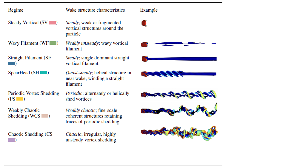
 λ2=−1
 ux

 60≤Re≤500
 0.02≤Ω≤1

 Re=200
 Ω=0.02
 Re=200
 ωx
 Ω=0.02

 y
 z
 x=xp+0.6
 ωx
 y
 z

 λ2=−1
 Re=220
 Ω=0.4
 x
 y
 u~x=ux−Uref∈[−0.1,0.1]
 L0/2

 Cd¯
 Ω
 60≤Re≤500
 Re
 Cd¯
 Re
 0.02≤Ω≤1
 Ω

 ‖Cl¯‖2
 Ω
 60≤Re≤500
 Cl¯
 ‖Cl‖2¯
 Re

 Ω
 60≤Re≤500
 Re=160
 Ω=0.02
 Ω=0.6
 x
 y
 ωx=±1
 λ2=−1
 Lr
 Re
 Lr
 Re=100
 250
 300
 y
 z
 x=xp+0.1
 Ω=0.4
 Ω=0.8
 Re=380
 Re=440
 u~x
 u~x>0
 u~x<0

 Tx¯
 Ω
 0.02≤Ω≤1
 60≤Re≤500
 Ω2/Tx¯
 ReΩ
 Re
 r2=0.9944

 Re=100
 220
 500
 I
 Str
 Ω
 Re
 Str1=4Ω/π
 y=Ω
 Str0=0.11

 Re=200
 Ω=0.4
 λ2=−1
 ux

 Re=100
 x
 ωx=±0.8

 Re=100
 200
 300
 0.02≤Ω≤1

 Re=100
 0.1≤Ω≤0.6
 ux
 Ω

 y
 z
 x=xp+0.6
 ωx
 y
 z

 ‖Cl¯‖2
 Re=100
 Re=200
 Cd¯
 Re=100
 Re=200
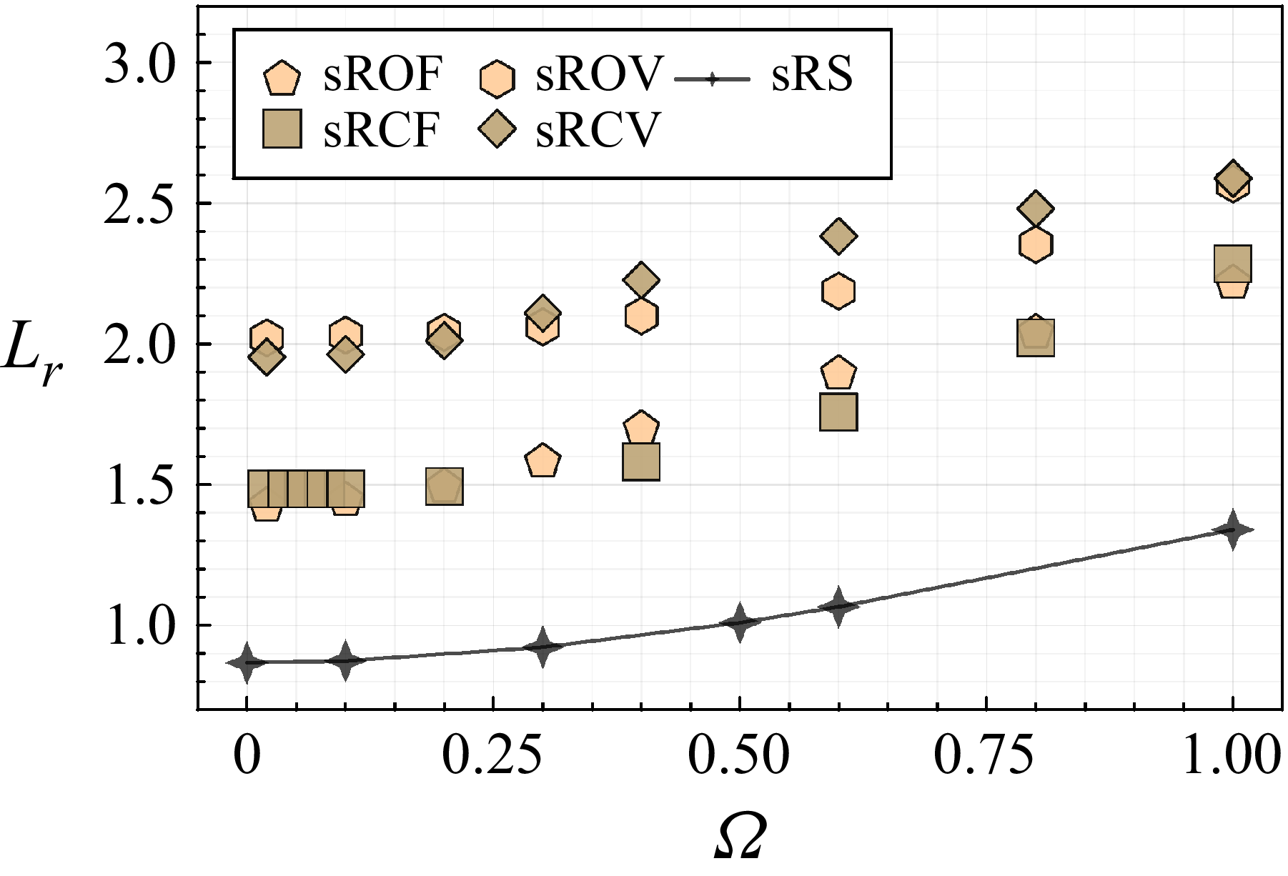
 Lr
 Re=100
 0.02≤Ω≤1

 Ω
 Str1
 Str=Ω
 Str0
 Str0=0.12
 Str0=0.11
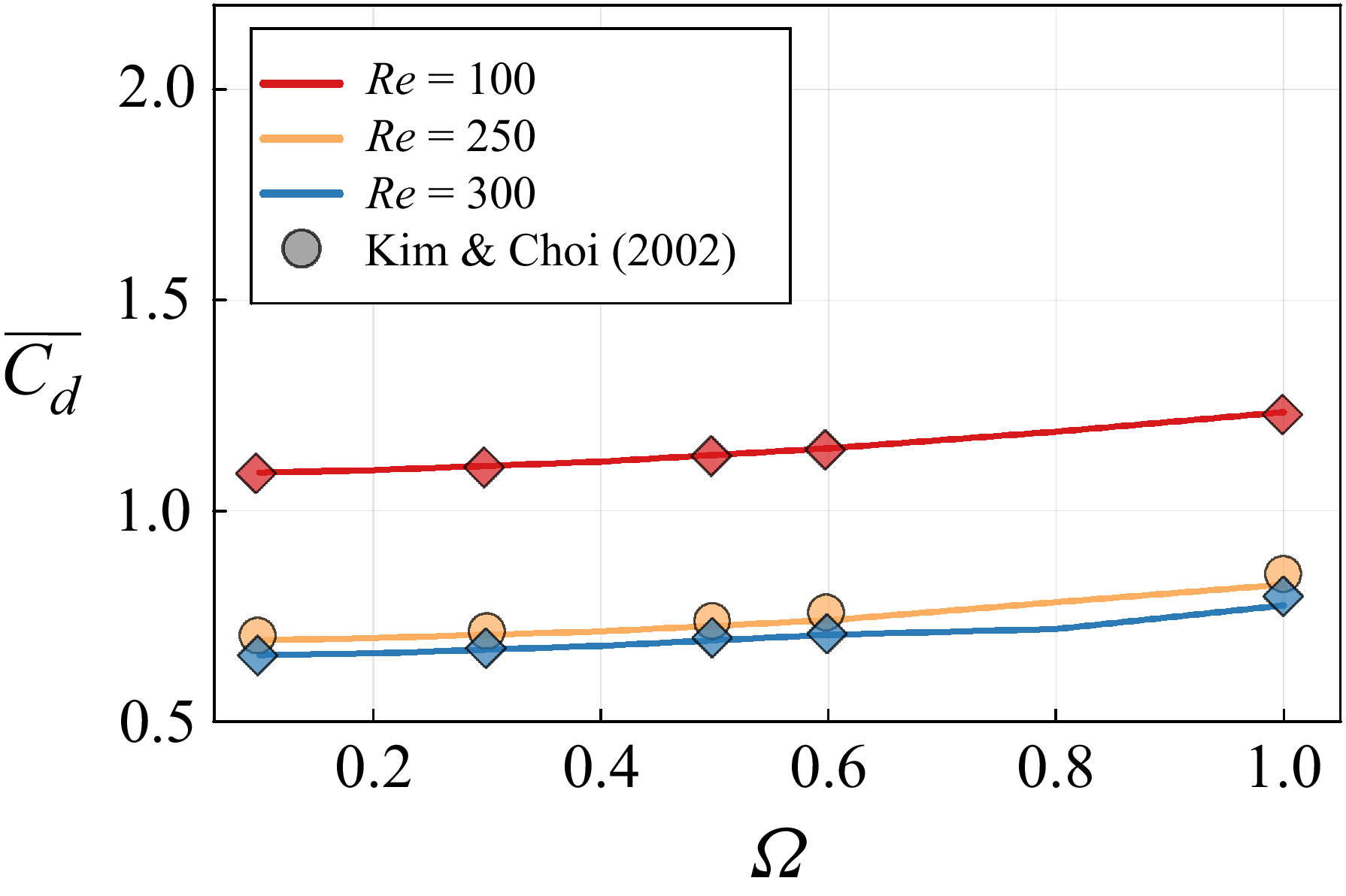
 Cd¯
 Ω
 Re=100
 250
 300

 y
 z
 x=xp+1.5
 ωx

 0.02≤Ω≤1
 60≤Re≤500
 λ2=−1
 ux

 λ2=−1
 Ω=1
 x
 y

 f(h)
 h
 Q>10
 Re
 hf(h)
 Ω=0.2
 0.6
 Ω
 f
 Re=100
 ⟨h⟩
 (Re,Ω)

 ωx
 ωx>0
 ωx<0
 Re=100
 Ω=1.0
 x=xp+1
 Re=300
 Ω=0.3
 x=xp+1.8
 Re=180
 Ω=0.4
 x=xp+0.8
 Re=200
 Ω=0.8
 x=xp+1.1

 Cd¯
 0.02≤Ω≤1
 Re=100
 200
 300
 cS
 χ
 Cd¯
 Re=200
 χ
 Cl¯
 Re=200
 cS
 Re=200
 Ω=0.4
 Ω=0.8
 ωx=±1
 Ω=0.2
 ωx
 λ2=−1
 ux

 Open access

