1. Introduction
Richtmyer–Meshkov instability (RMI) widely exists in natural and engineering flows (Brouillette Reference Brouillette2002; Zhou Reference Zhou2017a,Reference Zhoub) such as supernova explosions(Almgren et al. Reference Almgren, Bell, Rendleman and Zingale2006; Abarzhi et al. Reference Abarzhi, Bhowmick, Naveh, Pandian, Swisher, Stellingwerf and Arnett2019), inertial confinement fusion (ICF) (Lindl et al. Reference Lindl, Landen, Edwards, Moses and Team2014; Wang et al. Reference Wang2017b) and the interaction of a shock wave and a premixed or non-premixed flame (Billet Reference Billet2005; Massa & Jha Reference Massa and Jha2012; Attal & Ramaprabhu Reference Attal and Ramaprabhu2015; Jiang et al. Reference Jiang, Dong, Chen and Li2016a). When a perturbed interface separating two fluids with different densities was accelerated by an incident shock wave, the perturbed interface developed gradually, experienced linear growth, nonlinear growth and finally a turbulent mixing, and this hydrodynamic instability has been termed as RMI (Richtmyer Reference Richtmyer1960; Meshkov Reference Meshkov1969).
Richtmyer–Meshkov instability has been widely investigated theoretically (Dimotakis & Samtaney Reference Dimotakis and Samtaney2006; Vandenboomgaerde & Aymard Reference Vandenboomgaerde and Aymard2011; Liu et al. Reference Liu, Yu, Ye, Wang and He2014), experimentally (Motl et al. Reference Motl, Oakley, Ranjan, Weber and Anderson2009; Zhai et al. Reference Zhai, Liu, Qin, Yang and Luo2010, Reference Zhai, Si, Luo, Yang, Liu, Tan and Zou2012; Luo et al. Reference Luo, Si, Yang and Zhai2014, Reference Luo, Ding, Wang, Zhai and Si2015; McFarland et al. Reference McFarland, Reilly, Creel, McDonald, Finn and Ranjan2014; Zhai et al. Reference Zhai, Zou, Wu and Luo2018) and numerically (Lombardini, Pullin & Meiron Reference Lombardini, Pullin and Meiron2012, Reference Lombardini, Pullin and Meiron2014a,Reference Lombardini, Pullin and Meironb; Zhou Reference Zhou2017b) over the past few decades for different geometries. Relative to classic planar geometry, Bell–Plesset (BP) effects are present in cylindrical or spherical geometries with increasing convergence effects (Bell Reference Bell1951; Plesset Reference Plesset1954). The BP effects are reflected as additional perturbation growth from pure geometry, which leads to a more complex transition to turbulent mixing (Wang et al. Reference Wang, Wu, Ye, Zhang and He2013b, Reference Wang, Wu, Guo, Ye, Liu, Zhang and He2015). A large number of factors exist for the evolution of RMI, including initial conditions, Atwood numbers, Mach number, viscosity, etc. Random perturbations are always present on the interface in many practical engineering flows, which determines the eventual development of RMI (Thornber et al. Reference Thornber, Drikakis, Youngs and Williams2010, Reference Thornber2017; Zhou Reference Zhou2017b; Zhou, Groom & Thornber Reference Zhou, Groom and Thornber2020). The initial perturbations can be divided into single- and multi-mode perturbations, depending on the perturbed modes. For the multi-mode perturbation, the initial narrowband and broadband perturbed modes correspond to different growth rates via the physical processes of mode couplings and competitions, respectively. The broadband perturbed modes lead to a faster growth rate, which is more consistent with laser experiments (Thornber et al. Reference Thornber, Drikakis, Youngs and Williams2010; Groom & Thornber Reference Groom and Thornber2020). Different combinations of mixing materials can be summarized as the Atwood number effect, which describes the growth-reduction mechanism for the diffusion (Lombardini et al. Reference Lombardini, Hill, Pullin and Meiron2011). With the increase of the Atwood number, the asymmetry of bubbles and spikes becomes more and more apparent. Mach number effects might be controversial. With the increase of the initial Mach numbers, the scale separations would increase via increasing the perturbed velocity. However, the mixing parameter, the growth of the internal scale and the decaying rates of kinetic energy and enstrophy are found to be independent of the initial Mach numbers (Lombardini et al. Reference Lombardini, Pullin and Meiron2012; Tritschler et al. Reference Tritschler, Zubel, Hickel and Adams2014).
In extreme circumstances, chemical or nuclear reactions exist because of the high temperature, and the reactive instability could be classified into Rayleigh–Taylor instability (RTI) and RMI. The heat release within chemical reaction regions can change the thermodynamic parameters of flow fields and affect the temporal evolutions of RMI and RTI (Zhou et al. Reference Zhou, Clark, Clark, Glendinning, Skinner, Huntington, Hurricane, Dimits and Remington2019, Reference Zhou2021). The reactive RMI is of central importance in Scramjet engines, multiphase combustion in propulsion applications and dust cloud explosions like coal mines and food processing facilities. In Scramjet applications the enhanced mixing by RMI assures sufficient combustion within the residence times. The reactive RTI also applies in ultra-compact combustors in gas turbine systems, ICF and type Ia supernovae explosions (Chertkov, Lebedev & Vladimirova Reference Chertkov, Lebedev and Vladimirova2009; Zhou et al. Reference Zhou2021).
The combustion can be divided into premixed and non-premixed. For premixed combustion, the interactions of shock waves and perturbed flames are the core issues in reactive RMI, which originate from the heat release effect because of a chemical reaction. Under the effect of shock wave propagation, the heat release rates can increase nearly 30 times with the interactions of an inclined shock wave and a sinusoidally perturbed flame (Khokhlov et al. Reference Khokhlov, Oran, Chtchelkanova and Wheelerc1999). Kilchyk, Nalim & Merkle (Reference Kilchyk, Nalim and Merkle2011) noted that the fuel consumption rate of a premixed laminar flame increased rapidly, which was dominated by a one-dimensional shock compression effect. For chemical reaction effects on the evolution of perturbed interfaces, Massa & Jha (Reference Massa and Jha2012) employed the linear stability method to explore the evolution of a premixed flame with a single shock and concluded that the growth of small-scale perturbations can be suppressed by chemical reactions, which results from baroclinic effects. Jiang et al. (Reference Jiang, Dong, Chen and Li2016a) hypothesized two time scales for the evolution of a perturbed interface. One is the time scale for chemical reactions, and the other is the time scale for RMI. They confirmed that the time scale for RMI is dominant in the early stage, and the time scale for a chemical reaction is dominant in the late stage. Later, Jiang, Dong & Wu (Reference Jiang, Dong and Wu2016b) studied the multiple interactions of a flame interface with an incident shock wave to explore the effects of different initial perturbed amplitudes and thought that large amplitudes of the initial perturbed interface lead to large-scale vortex structures before the passages of reshock waves, which results in quick growth of the perturbed interface. After the successive impacts of multiple reshock waves, the chemical reaction weakens the baroclinic torque and begins to dominate, in contrast with the initial perturbed amplitudes.
In contrast to premixed combustion, non-premixed combustion is more challenging in experimental studies and engineering applications because of the difficulty of initial ignition and the uncertainty of chemical kinetic mechanisms (Zhou et al. Reference Zhou2021). However, benefiting from the developments of numerical simulations, important progress exists to uncover the intrinsic physical process of non-premixed combustion. Attal & Ramaprabhu (Reference Attal and Ramaprabhu2015) carried out two-dimensional numerical simulations of a single-mode chemical reacting RMI with hydrogen ( ${\rm H}_2$) and oxygen (
 ${\rm O}_2$) at different sinusoidal interface thicknesses, and the combustion waves impulsively accelerated any material line to promote the growth of the perturbed interfaces. Later, they also added the methane–air chemistry into an astrophysical code (FLASH) (Attal et al. Reference Attal, Ramaprabhu, Hossain, Karkhanis, Uddin, Gord and Royd2015). Bambauer, Hasslberger & Klein (Reference Bambauer, Hasslberger and Klein2020) carried out three-dimensional direct numerical simulations (DNS) of reactive RMI in plane geometry with multimodal initial perturbations, and found that the flame surface area is reduced by 50 %. Due to high computational costs, the detailed chemistry is not considered. Later, Bambauer et al. (Reference Bambauer, Chakraborty, Klein and Hasslberger2021) investigated the vortex dynamics and fractal structures in reactive RMI, and confirmed that baroclinic torque is dominant during shock-flame interactions. The interactions of the incident shock wave and combustion waves would result in non-planarity effects from combined RTI and RMI actions (Attal & Ramaprabhu Reference Attal and Ramaprabhu2015; Zhou Reference Zhou2017a). Nevertheless, few works have focused on the chemical reaction effects on mixing transition and turbulent statistics with detailed chemistry in three-dimensional numerical simulations, especially within the frame of cylindrical or spherical geometries. The curved geometry is widely at present in the applications of ICF, supernova collapse and explosive detonations (Lombardini et al. Reference Lombardini, Pullin and Meiron2014a; Zhou Reference Zhou2017b). Hence, in this paper we select the cylindrical shock wave and perturbed interface to carry out DNS of RMI with and without chemical reactions and uncover the statistical characteristics during the process of transition and late-time turbulent mixing.
The rest of the paper is organized as follows. In § 2 we introduce the detailed computational settings, including the governing equations, initial conditions and chemical reactions. Next, in § 3 the numerical results are presented, and we discuss the shock propagation, grid resolution, mixing width and other turbulent statistics. The conclusions are summarized in § 4.
2. Numerical settings
We perform DNS of RMI with and without chemical reactions using our open-source software Opencfd-Comb. A sixth-order finite difference scheme (OMP6) (Li, Leng & He Reference Li, Leng and He2013) is adopted to discretize the convective terms, and an eighth-order central difference scheme is adopted to discretize the viscous terms. In addition, we employ the standard third-order Runge–Kutta method as the time-marching scheme. The software Opencfd-Comb has been widely validated in our previous work, including supersonic jet flows (Fu et al. Reference Fu, Yu, Yan and Li2019a,Reference Fu, Yu, Yan and Lib) and RMI (Fu, Yu & Li Reference Fu, Yu and Li2020; Li et al. Reference Li, Fu, Yu and Li2021).
2.1. Governing equations
The conservation form of three-dimensional compressible Navier–Stokes equations with multi-species of miscible gases reads as
 \begin{gather} \frac{\partial \rho}{\partial t}+\boldsymbol{\nabla}\boldsymbol{\cdot}\left( \rho {\boldsymbol{u}} \right)=0, \end{gather}
 \begin{gather} \frac{\partial \rho {\boldsymbol{u}}}{\partial t}+\boldsymbol{\nabla}\boldsymbol{\cdot}\left( \rho {\boldsymbol{u}} {\boldsymbol{u}} \right)={-}\boldsymbol{\nabla}\left( p \boldsymbol{\delta} - \boldsymbol{\sigma} \right), \end{gather}
 \begin{gather} \frac{\partial E}{\partial t}+\boldsymbol{\nabla}\boldsymbol{\cdot}\left( \rho \left( E+p \right) {\boldsymbol{u}} \right)=\boldsymbol{\nabla}\left( \boldsymbol{\sigma}\boldsymbol{\cdot}{\boldsymbol{u}}+ {\boldsymbol{q}}\right)+Q_s, \end{gather}
 \begin{gather} \frac{\partial \rho Y_m}{\partial t}+\boldsymbol{\nabla}\boldsymbol{\cdot}\left( \rho Y_m {\boldsymbol{u}} \right)=\boldsymbol{\nabla}\boldsymbol{\cdot}\left( \rho D_m \boldsymbol{\nabla} Y_m \right)+\dot{W}_m, \end{gather}
where  $\rho$ denotes the mixture density,
 ${\boldsymbol {u}}$ denotes the velocity vector,
 $p$ is the static pressure,
 $\boldsymbol {\delta }$ is the Kronecker function and
 $Y_m$ is the mass fraction of the mth species of mixture. Here
 $E$ is the total energy per unit volume, which is defined as
 \begin{equation} E=\frac{1}{2}\rho {\boldsymbol{u}}^2+\sum_{m=1}^N \rho_m h_m-p, \end{equation}
where  $N$ denotes the total number of reactive species,
 $\rho _m$ is the mth-species density and
 $h_m$ is the mth-species enthalpy. According to Stokes’ hypothesis, the bulk viscosity is assumed to be zero (Graves & Argrow Reference Graves and Argrow1999), and the viscous stress tensor
 $\boldsymbol {\sigma }$ for a Newtonian fluid is defined as
 \begin{equation} \sigma_{ij}=\mu\left( \frac{\partial u_i}{\partial x_j}+\frac{\partial u_j}{\partial x_i}-\frac{2}{3}\theta\delta_{ij} \right), \end{equation}
where  $\theta =\partial u_k / \partial x_k$ corresponds to the compression or expansion of fluid elements and
 $\mu$ is the mixture viscosity. According to Fourier's law and Fick's law, the conductive heat flux
 $\boldsymbol {q}$ is given as
 \begin{equation} \boldsymbol{q}=\kappa\boldsymbol{\nabla} T+ \rho\sum_{m=1}^N D_m h_m \boldsymbol{\nabla} Y_m, \end{equation}
where  $\kappa$ is the thermal conductivity of the mixture,
 $T$ is the temperature of the mixture and
 $D_m$ is the mth-species effective binary diffusion coefficient. Here
 $Q_s$ (J (m
 $^3$ s)
 $^{-1}$) is the heat release rate per unit volume for the chemical reaction, which can be computed by
 \begin{equation} Q_s={-}\sum_{m=1}^N\dot{W}_m h_m^0, \end{equation}
where  $h_m^0$ represents the mth-species enthalpy production rate per unit mass and
 $\dot {W}_m$ represents the mass production rate per unit volume. According to the Dalton's law of partial pressures and the isothermal hypothesis, the equation of state can be expressed as
 \begin{equation} p=\sum_{m=1}^N \rho_m R_m T=\sum_{m=1}^N \rho_m \frac{R_0}{M_m} T, \end{equation}
where  $R_0=8.314$ J (mol K)
 $^{-1}$ is the universal gas constant and
 $M_m$ is the mth-species molar mass. Hence, the molarity can be defined as
 $[ X_m ]=\rho _m/M_m$. The specific heat at constant pressure per unit mass
 $C_p$, enthalpy per unit mass
 $h$ and entropy
 $S$ per unit mass are computed through the following fitting polynomials (Gordon & McBride Reference Gordon and McBride1971):
 \begin{gather} \frac{C_{p_m}}{R_m}=A_m+B_m T+C_m T^2+D_m T^3+E_m T^4, \end{gather}
 \begin{gather} \frac{h_m}{R_m}=A_m T+ \frac{1}{2} B_m T^2 + \frac{1}{3} C_m T^3+ \frac{1}{4} D_m T^4 + \frac{1}{5} E_m T^5 + F_m, \end{gather}
 \begin{gather} \frac{S_m}{R_m}=A_m \ln T+B_m T+\frac{1}{2} C_m T^2+\frac{1}{3} D_m T^3+\frac{1}{4} E_m T^4+G_m. \end{gather}
Here  $A_m, B_m, C_m, D_m, E_m, F_m, G_m$ are the corresponding fitting coefficients and
 $h_m^0=R_m F_m$. Hence, the specific heat at a constant pressure of the mixture
 $C_{p_{mix}}$ and the mixture enthalpy
 $h_{mix}$ can be computed through
 \begin{equation} C_{p_{mix}}=\sum_{m=1}^N C_{p_m} Y_m, \quad h_{mix}=\sum_{m=1}^N h_m Y_m. \end{equation}
The mth-species viscosity  $\mu _m$, thermal conductivity
 $\kappa _m$ and effective binary diffusion coefficient
 $D_m$ can be computed by fitting polynomials from CHEMKIN (Kee, Rupley & Miller Reference Kee, Rupley and Miller1989). Therefore, the mixture viscosity
 $\mu$ and the thermal conductivity of the mixture
 $\kappa$ can be obtained by
 \begin{equation} \mu=\sum_{m=1}^N\frac{X_m \mu_m}{\sum_{j=1}^K X_j \varPhi_{mj}}, \quad \kappa=\frac{1}{2}\left( \sum_{m=1}^N X_m \kappa_m+ \frac{1}{\sum_{m=1}^N X_m / \kappa_m } \right). \end{equation}
Here,
 \begin{equation} \varPhi_{mj}=\frac{1}{\sqrt{8}}\left( 1+\frac{M_m}{M_j} \right)^{{-}1/2}\left[ 1+\left( \frac{\mu_m}{\mu_j}\right)^{1/2}\left( \frac{M_j}{M_k} \right)^{1/4} \right]^2. \end{equation}
In addition, the mth-species effective binary diffusion coefficient  $D_m$ can be obtained by
 \begin{equation} D_m=\frac{1-X_m}{\sum_{j=1,j\neq m}^N X_j/D_{jm}}, \end{equation}
where  $X_m$ is the mth-species volume fraction.
2.2. Initial condition
Consistent with our previous work (Fu et al. Reference Fu, Yu and Li2020), we employ the multimode initial interfacial perturbation proposed by Lombardini et al. (Reference Lombardini, Pullin and Meiron2014a). Although the initial condition effects are crucial for nonlinear growth or late-time fully developed turbulent flows (Budzinski, Benjamin & Jacobs Reference Budzinski, Benjamin and Jacobs1994; Youngs Reference Youngs2013; Vandenboomgaerde et al. Reference Vandenboomgaerde, Souffland, Mariani, Biamino, Jourdan and Houas2014), the initial conditions of the two cases we carried out in this paper are the same. Hence, we just ignore the initial condition effects and focus on the effect of a chemical reaction.
The perturbed surface separating fluids with different densities are defined as  $r=\zeta _0(\theta,\phi )$, and the mass fraction field
 $\psi (r,\theta,\phi )$ can be obtained by
 \begin{equation} \psi(r,\theta,\phi)=\frac{1}{2}\left\{ 1-\tanh\left[ \frac{r-\zeta_0(\theta,\phi)}{L_r} \right] \right\}, \end{equation}
where  $\zeta _0(\theta,\phi )=R_0-a_0 |f(R_0,\theta,\phi )|$,
 $f(R_0,\theta,\phi )=\sum _{l=0}^M \sum _{m=-l}^l f_{lm} Y_{lm}(\theta,\phi )$,
 $f_{lm}=\sqrt {( 2l+1 )C_l}\cos ( 2{\rm \pi} \omega _l^m )/\sqrt {\sum _{i=-l}^l \cos ( 2{\rm \pi} \omega _l^i )}$. For more detailed definitions, we refer the reader to Lombardini et al. (Reference Lombardini, Pullin and Meiron2014a) and Fu et al. (Reference Fu, Yu and Li2020). Our main computational domain is
 $L_x \times L_y \times L_z=20 \,{\rm mm} \times 20 \,{\rm mm}\times 20 \,{\rm mm}$ with a homogeneous Cartesian mesh. We set up periodical boundary conditions for the
 $z$ direction, and buffer regions are adjoined to the main computational domain in the
 $x$ and
 $y$ directions with a sparse mesh to avoid the effect of shock reflection at the boundary. The grid resolution in the main computational domain is
 $1024^3$. For the initial perturbed interface, we set the position located at
 $R_0=7\,{\rm mm}$, the characteristic thickness
 $L_r=0.2\,{\rm mm}$, the dominant spherical wavenumber
 $l_0=20$, the variance
 $\sigma _0=l_0/15$ and
 $a_0=0.375\,{\rm mm}$.
We show the isosurface of the mass fraction of hydrogen  $Y_H$ with
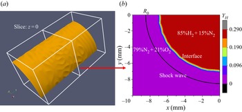
 $5\,\%$ at the initial status in figure 1(a), and only a quadrant is selected to exhibit the perturbed interface. To further demonstrate the multi-mode characteristics, a contour slice at the cross-section of
 $z=0$ is shown in figure 1(b). A perturbed interface with a characteristic thickness is apparent, which assures the development of late-time turbulent mixing.
(a) Isosurface of the mass fraction of hydrogen  $Y_H$ with
 $5\,\%$ at the initial status. (b) Contour slice of the mass fraction of hydrogen
 $Y_H$ at the cross-section of
 $z=0$, and the black convergent curve denotes the position of the shock wave.

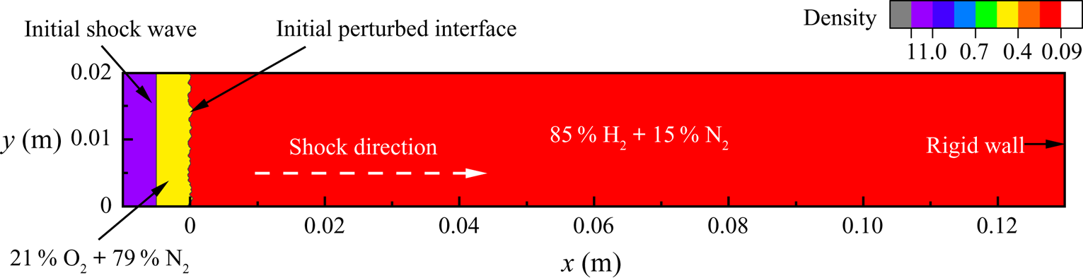
To be consistent with the one-dimensional shock tube experiment (Vetter & Sturtevant Reference Vetter and Sturtevant1995; Leinov et al. Reference Leinov, Malamud, Elbaz, Levin, Ben-Dor, Shvarts and Sadot2009) and other numerous simulations (Hill, Pantano & Pullin Reference Hill, Pantano and Pullin2006; Lombardini et al. Reference Lombardini, Hill, Pullin and Meiron2011; Bengoechea et al. Reference Bengoechea, Stein, Reiss and Sesterhenn2014), an initial convergent shock Mach number is set as  $M_s=1.5$ with the position of
 $R_{s}=8.5\,{\rm mm}$. The inner species of the perturbed cylinder are full of 85 %
 ${\rm H}_2$ and 15 %
 ${\rm N}_2$, with a pressure of 101 325 Pa and a temperature of 800 K. The outer species of the perturbed cylinder are full of 79 %
 ${\rm N}_2$ and 21 %
 ${\rm O}_2$, and their pressure and temperature are the same as those of the inner species. Other thermal variables and the velocity vector can be computed according to the Rankine–Hugoniot condition (Anderson Reference Anderson2010), and they are listed in the table 1.
Flow parameters at the initial status;  $U_r$ is the radial velocity.

2.3. Chemical reaction computations
In our numerical simulations we adopted an updated 9-species ( ${\rm H_2}$,
 ${\rm H}$,
 ${\rm O_2}$,
 ${\rm O}$,
 ${\rm OH}$,
 ${\rm HO_2}$,
 ${\rm H_2} O_2$,
 ${\rm H_2} O$ and
 ${\rm N_2}$) and 19-reaction model proposed by Li et al. (Reference Li, Zhao, Kazakov and Dryer2004). The kinetic model of the
 $H_2$/
 $O_2$ reaction can be written uniformly as
 \begin{equation} \sum_{i=1}^9\nu_{ij} B_i \rightleftharpoons \sum_{i=1}^9\nu'_{ij} B_i,\quad (j=1,2,\ldots,19), \end{equation}
where  $B_i$ denotes the ith species and
 $\nu _{ij}$ and
 $\nu '_{ij}$ are stoichiometric numbers of reactants and products, respectively. The mass production rate of the ith species because of the jth chemical reaction can be computed as
 \begin{equation} \left( \frac{{\rm d} \rho_i}{{\rm d} t} \right)_j=M_i \left( \nu'_{ij}-\nu_{ij} \right)\left( \eta_j - \eta'_j \right). \end{equation}
Here,  $\eta _j$ denotes the forward reaction rate, which is computed from the Arrhenius formula;
 $\eta '_j$ denotes the reversal reaction rate, which needs to involve the chemical equilibrium constant. Therefore, the mass production rate for the ith species is obtained by summing all element reactions,
 \begin{equation} \dot{W}_i=\sum_{j=1}^N\left(\frac{{\rm d} \rho_i}{{\rm d} t}\right). \end{equation}
3. Results and discussions
3.1. Shock propagation
According to Guderly's theory, there exists a similarity exponent  $\alpha$ to bridge a connection of the strong shock position
 $R_s(t)$ and propagation time
 $t$ as
 $R_s(t)\sim ( 1-t/t_s )^\alpha$ (Guderley Reference Guderley1942), and
 $t_s$ is the time when a strong shock reaches the origin. The similarity exponent can be obtained by solving ordinary differential equations, and it depends on the ratio of specific heat for cylinder geometry (Dyke & Guttmann Reference Dyke and Guttmann1982; Chisnell Reference Chisnell1998; Lombardini & Pullin Reference Lombardini and Pullin2009). In our numerical simulations with or without chemical reactions, the fitted slopes are 0.800, which is consistent with the theoretical prediction.
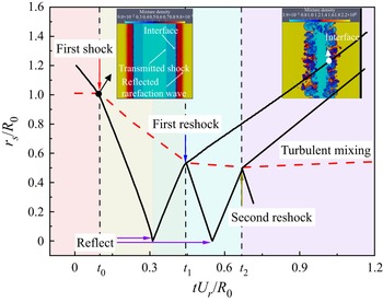
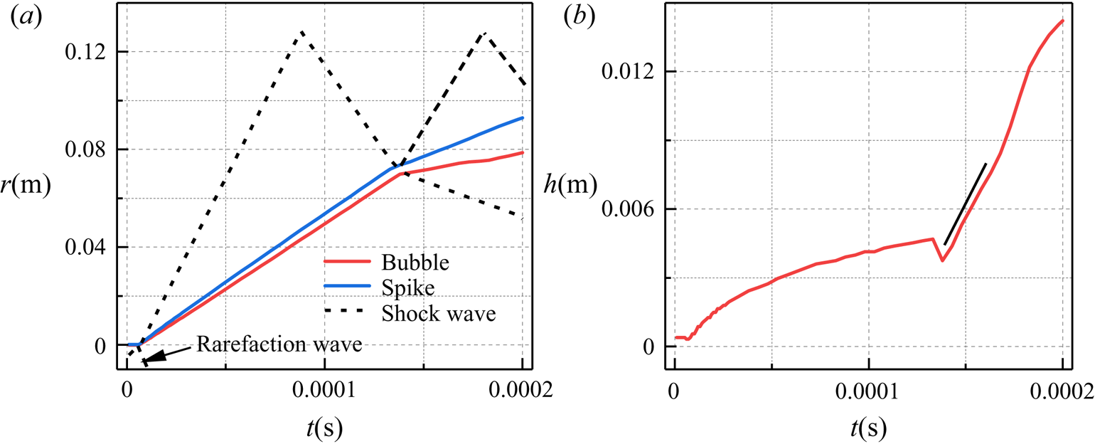
The shock propagation diagram shown in figure 2 provides an abundant physical configuration of the temporal evolutions of cylindrical RMI. Over time, the strong shock propagates to the origin convergently. The speed of shock propagation is not constant, although the curve in figure 2 seems to be straight visually. After the first interaction of the incident shock and perturbed interface ( $t_0$), a transmitted shock propagating to the origin and a reflected expansion wave propagating outwardly are produced, and the perturbed interface accelerates inwardly. The reflected expansion wave propagates divergently to the boundary, and its propagation time in coarse grids is long enough to avoid pollution on the flow field in our numerical simulations. The transmitted shock converges to the origin and then reflects at the origin outwardly. Subsequently, the interaction of the shock wave and perturbed interface reoccurs, and the acceleration direction of the perturbed interface is reversed. The light-to-heavy fashion would generate a transmitted shock propagating outwardly and a reflected shock propagating inwardly (Lombardini et al. Reference Lombardini, Pullin and Meiron2014a). After the first reshock (
 $t_1$), the fluid instability would develop quickly, along with transition and turbulent mixing. Sufficient mixing is needed for an apparent chemical reaction, and the instant of the first reshock is marked as the starting time for the apparent chemical reaction effect. During the process of shock propagating within the mixing regions, the velocity fluctuations would be weakened, which is represented by the smaller turbulent kinetic energy, the smaller enstrophy, the smaller palinstrophy and the smaller viscous dissipation rates. In addition, the weakened fluctuations are also reflected by the inverse energy cascade process. The specific discussions are exhibited in the later sections in detail. The same shock propagation diagram is repeated after the first reshock, but the shock strength is smaller over time. In our numerical simulations and temporal analysis, we focus on the temporal ranges from the instant before the first reshock and the instant after the second reshock (
 $t_2$) to uncover the physical configurations of the perturbed interface, and they are marked up with a background colour of light cyan and purple in the subsequent figures.
Diagram of shock propagation, with first shock, reflection, reshock and turbulent mixing. Here  $r_s$ denotes the positions of the shock wave (solid black line) and the inner radius of the mixing regions (dashed red line). The insets are two-dimensional contour slices of the mixture density without a chemical reaction. Their instants are after the first shock and eventual mixing.

The diagram of the shock propagation with a chemical reaction is much the same as the case without a chemical reaction. Their diagrams of shock propagation are similar to the classic RMI with cylinder geometry in numerical simulations (Hill et al. Reference Hill, Pantano and Pullin2006; Lombardini et al. Reference Lombardini, Hill, Pullin and Meiron2011; Wu, Liu & Xiao Reference Wu, Liu and Xiao2021) and experiments (Houas & Chemouni Reference Houas and Chemouni1996; Si et al. Reference Si, Long, Zhai and Luo2015; Ding et al. Reference Ding, Li, Sun, Zhai and Luo2019). Because of the complex definition of the mixing width involved in a chemical reaction, the interface motion will be discussed in detail in the subsequent section.
3.2. Grid resolution
The criteria for transition to turbulent mixing have always been an indeterminate issue for RMI for a long time, and the transition criteria involve spatial and temporal scales of large separations (Zhou et al. Reference Zhou2003; Zhou Reference Zhou2007, Reference Zhou2017a). Turbulent mixing means rapid mixing of momentum and concentration at the molecular scale (Dimotakis Reference Dimotakis2000), which is beneficial to a chemical reaction. After reshock, the flow quickly tends to transition to a turbulent state (Tomkins et al. Reference Tomkins, Balakumar, Orlicz, Prestridge and Ristorcelli2013). Hence, we may select the time after the reshock as turbulent mixing from the perspective of temporal criteria. For spatial criteria, we focus on the characteristic length scales (Taylor microscale  $\lambda$ and Kolmogorov viscous scale
 $\eta$) to evaluate whether the flow has developed a turbulent field (Cook & Zhou Reference Cook and Zhou2002; Yan et al. Reference Yan, Li, Wang and Yu2019). Their definitions are
 \begin{equation} \lambda_r=\left[ \frac{\left\langle u_r^2\right\rangle}{\left\langle \left( \partial u_r / \partial x_r \right)^2 \right\rangle} \right]^{1/2}, \quad \eta=\left( \frac{\nu^3}{\left\langle\epsilon\right\rangle} \right)^{1/4}, \end{equation}
where  $\epsilon$ is the viscous dissipation rate and
 $r$ represents the radial direction. Hence, the Reynolds number based on the Taylor microscale
 $Re_\lambda$ can be defined as
 \begin{equation} Re_\lambda=\frac{\left\langle \rho \right\rangle \lambda_r \left[ \left\langle u_r^2 \right\rangle \right]^{1/2}}{\mu}. \end{equation}
Dimotakis (Reference Dimotakis2000) proposed that fully developed turbulent flow requires a Taylor Reynolds number  $Re_\lambda \geq 100\text {--}140$. However, the critical Reynolds number is sufficient but not necessary (Robey et al. Reference Robey, Zhou, Buckingham, Keiter, Remington and Drake2003). The temporal scales for turbulent cascade are not negligible, especially for the formation of the inertial subranges. The minimum state proposed by Zhou (Reference Zhou2007) requires the Taylor Reynolds number
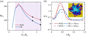
 $Re_\lambda \geq 560$. In our numerical simulations we calculate the Taylor microscale within the mixing region over time and show the Taylor Reynolds number
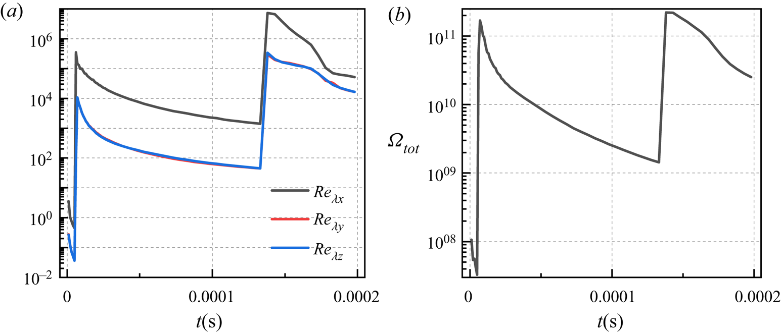
 $Re_\lambda$ in figure 3. After reshock, the Taylor Reynolds number
 $Re_\lambda$ gradually increases in the early period, which corresponds to the transition to turbulent mixing. Then, the Taylor Reynolds number
 $Re_\lambda$ gradually decreases because of the apparent role of viscosity. The time diagrams of the two cases are similar, and their maximums satisfy the requirements of the critical Taylor Reynolds number. We also compute the Kolmogorov viscous scale at different radii and show the ratio of the grid scale and Kolmogorov viscous scale at two instants in figure 3. According to the criteria of DNS (Pope Reference Pope2010), the grid resolution is enough to capture the vast majority of scales.
(a) Taylor Reynolds number  $Re_\lambda$ over time, where the black spheres correspond to the times of (b). The lilac area corresponds to the status after reshock. (b) The ratio of grid scale and Kolmogorov viscous scale over radius at two different times. The inset shows the contour slice of mixture density on the
 $x$–
 $y$ slice at
 $t=40\,\mathrm {\mu }{\rm s}$ without a chemical reaction, which illustrates inner and outer radii of the mixing region. Here NCR indicates a non-chemical reaction, and CR indicates a chemical reaction.

In contrast to the case without a chemical reaction, the Reynolds number of the case with a chemical reaction is smaller, and the Kolmogorov viscous scale is larger. This phenomenon means that turbulent flows with chemical reactions are less developed, and the main reason is the heat release effect of the chemical reaction.
3.3. Mixing width
Most studies have dealt with the mixing of two fluids, and the mixing width has always been defined as the regions of mass fraction with threshold 1 %–99 % (or 5 %–95 %) (Mikaelian Reference Mikaelian2005; Zhou Reference Zhou2017a; Mikaelian & Olson Reference Mikaelian and Olson2020). The classic definition of mixing width cannot be successfully applied to our numerical simulations involving more fluids or elements, but we indeed need a specific definition of mixing width for a chemical reaction. From the element diffusion point of view, hydrogen diffuses out from the inside, and oxygen diffuses from the outside. According to this physical process, we propose the following two definitions of mixing width.
The first definition deals with species involving only hydrogen and oxygen with a threshold of 5 %. More precisely, the total fraction of species H and species H2 with threshold 5 % is employed to define the outer radius  $r_2$, and the total fraction of species O and species O2 with threshold 5 % are employed to define the inner radius
 $r_1$. Hence, the mixing width can be obtained by the difference between the outer and inner radii.
In contrast, the second definition deals with species involving all hydrogen and oxygen with a threshold of 5 %. Rather, the total fraction of hydrogen from species H, species H2, species OH, species H2O, species H2O2 and species HO2 with threshold 5 % is used to define the outer radius  $r_1$. The total fraction of oxygen from species O, species O2, species OH, species H2O, species H2O2 and species HO2 with a threshold of 5 % is used to define the inner radius
 $r_2$. The mixing width is the difference between the outer and inner radii. The above two definitions are the same for the case without a chemical reaction. Of course, 1 % can also be selected as the threshold, and negligible differences in statistical results exist in our numerical simulations (Ramaprabhu et al. Reference Ramaprabhu, Dimonte, Woodward, Fryer, Rockefeller, Muthuraman, Lin and Jayaraj2012).
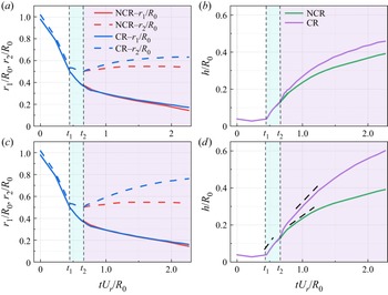
Based on the above two definitions, we compute the inner radius  $r_1$ and outer radius
 $r_2$ of mixing regions with and without chemical reactions in figure 4(a,c). The inner radii based on the two definitions are nearly the same with and without chemical reactions, and the difference lies in the outer radius. The outer radius without a chemical reaction approaches a constant in the late stage. However, with a chemical reaction, the outer radius increases gradually over time, and the growth rate of the outer radius based on the second definition is larger than that based on the first definition. The principal reason is that the chemical reaction in our simulation is non-premixed, and the chemical reaction mainly occurs around the outer radius. The mixing widths obtained from the corresponding outer and inner radii with and without chemical reactions are shown in figure 4(b) (based on the first definition) and (d) (based on the second definition). Similar to the regularities of the outer radius, the growth rate of the mixing width with a chemical reaction is larger than that without a chemical reaction. The discrepancy becomes apparent from the moment of reshock, which indicates the occurrence of the chemical reaction because of sufficient mixing of reactants.
(a) The inner radius  $r_1$ and outer radius
 $r_2$ of mixing regions based on the first definition with and without chemical reactions over time. (b) The mixing widths based on the first definition with and without chemical reactions over time. (c) The inner radius
 $r_1$ and outer radius
 $r_2$ of mixing regions based on the second definition with and without chemical reactions over time. (d) The mixing widths based on the second definition with and without chemical reactions over time. The black dashed lines mark the stages of the linear growth.

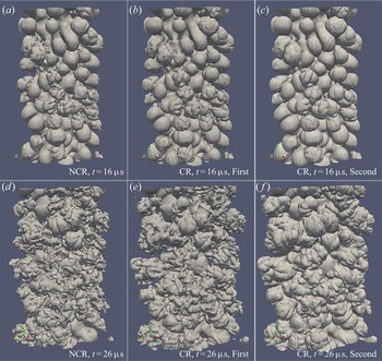
We select the isosurfaces of the hydrogen fraction of the first and second definitions at two typical instants to show the discrepancy of the above two definitions in figure 5. Chemical reactions mainly occur around the outer radius, and small-scale structures with more sufficient mixing are easily dissipated. Hence, large-scale bubbles around the outer radius are dominant with a chemical reaction. Comparing the isosurfaces in figure 5(a–c), we find that the second definition is superior for exhibiting large-scale bubbles. The isosurface in figure 5(b) shows that the first definition misses some diffusion information of some species and leads to incorrect spatial distributions and mixing width. The similar large- and small-scale structures without a chemical reaction and with a chemical reaction based on the first definition in figure 5 confirm this conclusion. At other instants, the regulations and discrepancies of their spatial distributions are similar, and the numerical results at  $t=26 \,\mathrm {\mu }{\rm s}$ in the late stage also illustrate that the second definition is suitable for the mixing width with multiple species mixing. Hence, we select the second definition to define the mixing width in later sections.
The three-dimensional isosurfaces of hydrogen corresponding to the first definition of the mixing width at  $t=16 \,\mathrm {\mu }{\rm s}$ without a chemical reaction (a) and with a chemical reaction (b), and at
 $t=26 \,\mathrm {\mu }{\rm s}$ without a chemical reaction (d) and with a chemical reaction (e). The three-dimensional isosurfaces of all hydrogen elements including species H, species H2, species OH, species H2O, species H2O2 and species HO2, corresponding to the second definition of the mixing width with a chemical reaction at
 $t=16 \,\mathrm {\mu }{\rm s}$ (c) and at
 $t=26 \,\mathrm {\mu }{\rm s}$ ( f).

In RMI with cylinder geometry, a simple prediction model with an incompressible equation that captures the convergence effect (Mikaelian Reference Mikaelian2005) is
 \begin{equation} h=c A \triangle v t R_0/R, \end{equation}
where  $c$ is a constant,
 $A$ is the Atwood number,
 $\triangle v$ is the velocity difference before and after the shock wave and
 $R$ is the cylinder radius. This model has been validated in cylindrical convergent RMI with two fluids (Mikaelian Reference Mikaelian2005; Lombardini & Pullin Reference Lombardini and Pullin2009). This linear model is also validated in the present numerical simulations with and without chemical reactions in figure 4(d), except around the instants of the first and second reshock. From the instant of the interaction of the reshock and the inner radius of the mixing regions, the mixing regions are compressed, and then stretched after the interaction of the reshock and the outer radius. The linear growth of the mixing regions is destroyed by the compressing and stretching effects. These effects are more apparent, especially around the second reshock than the first reshock, and the main reason may come from the wider mixing regions. Subsequently, the growth of the mixing width would be linear. After a full development with sufficient time, the growth of the mixing width might be self-similar.
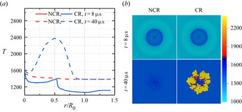
There may exist many possible reasons for the quicker growth of the mixing width with a chemical reaction. First, a large number of products are present around the outer radius, and the Atwood number is changed dramatically. The Atwood number effect may be one of the prime causes. Although Dimonte & Schneider (Reference Dimonte and Schneider2000) provided the Atwood number dependence, we could not obtain a specific Atwood number dependence for the growth rate of mixing widths because of various Atwood numbers in the process of a chemical reaction. Second, the combustion waves would be produced within the mixing regions, and propagate inwardly and outwardly. The heat release of chemical reactions leads to a large temperature difference, which is suitable for mixing. To confirm this explanation, we show the temperature profiles over radius at the instant of reshock and the late time in figure 6(a) and contour slices of the temperature distribution with and without chemical reactions in figure 6(b). After reshock, the mixing is not sufficient for a chemical reaction, and the temperature profiles with and without chemical reactions overlap at  $t=8\,\mathrm {\mu }{\rm s}$. In the late stage, the temperature increases dramatically along with heat release, especially in the mixing regions. However, the temperature rise without a chemical reaction is smaller.
(a) Temperature profiles over radius with and without chemical reactions at different times, and the temperature profiles with and without chemical reactions overlap at  $t=8\,\mathrm {\mu }{\rm s}$. (b) Contour slices of the temperature distribution on the
 $x$–
 $y$ slice, corresponding to the status in (a).

3.4. Chemical reaction description
This section highlights the statistical characteristics of the chemical reaction, including the internal energy, heat release and consumption and production rates. In the early stage, it needs to absorb energy from flow fields to promote the development of the chemical reaction. Subsequently, it releases heat into flow fields to increase the temperature. However, the propagation of shock waves also leads to an increase in internal energy. Hence, we investigate these statistical characteristics individually.
As a part of total energy, the internal energy is extracted from (2.2) as
 \begin{equation} Ei=\sum_{m=1}^N \rho_m h_m-p. \end{equation}
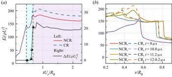
We show the mean internal energy within the mixing regions with and without chemical reactions in figure 7. There exists an apparent discrepancy of the internal energy with and without chemical reactions, especially in the late stage. The mean internal energy with a chemical reaction is larger due to the heat release effect. With the development of mixing width, the mean internal energies within the mixing regions with and without chemical reactions decrease. The decay of the mean internal energy in figure 7(a) originates from the increase of the mixing regions. The chemical reaction would be weakened with the decrease of the fuels around the mixing centre in the late time. Non-reactive oxygen is rolled up into the mixing regions, and is transported towards the mixing centre. With the development of the mixing regions, more time is needed for the oxygen transportation to reach a fully mixed status. The discrepancy can not be negligible after the first reshock, and becomes apparent subsequently. The radial distribution in figure 7(b) indicates that the increased internal energy induced by a chemical reaction is smaller than that by shock propagation in the current situation. We infer that if the Mach number is larger, the internal energy change induced by shock propagation would be more dominant.
(a) The mean internal energy with and without chemical reactions over time, and their difference is shown on the right vertical axis. (b) The internal energy with and without chemical reactions over radius at four different times corresponding to (a).

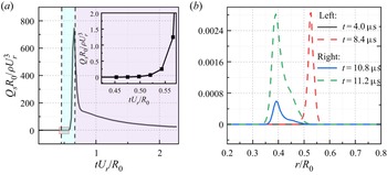
The internal energy change cannot be directly associated with the chemical reaction because the presence of viscosity also transfers energy from kinetic energy into internal energy. The heat released by a chemical reaction is explored directly in figure 8. The heat release only originates from the chemical reaction, and we focus on its temporal evolution and radial distributions of the case with a chemical reaction. Consistent with the internal energy change, the mean heat release comes from a negative value in the early stage to a positive value after the first reshock. The rapid development of the mean heat release after the first reshock is consistent with transition and turbulent mixing development. Both the subsequent decay of the mean heat release in figure 8(a) and the lower values around the outer radius in figure 8(b) come from the development of the mixing regions. The radial distribution of the mean heat release after the first reshock in figure 8(b) reveals that the chemical reaction releases heat into flow fields, and the mean heat release increases rapidly in the subsequent times.
(a) The mean heat release over time, and the inset shows its temporal evolution after the first reshock. (b) The mean heat release over radius at four different times.

In order to evaluate the spatial distribution of heat release, we show the contour slices of heat release at the plane of  $z=L_z/2$ at different instants in figure 9. In the early stage of figure 9(a) the value of the heat release is negative, and it means that the chemical reaction absorbs energy from the flow fields. After the first reshock (figure 9b), the value of the heat release is positive, which indicates the beginning of the chemical reaction effect. With the development of transition and turbulent mixing, the heat release increases dramatically. Due to the initial non-premixed configuration, the chemical reaction only appears within the mixing regions.
Contour slices of the heat release at three different instants.

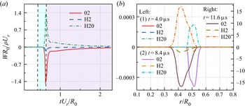
The consumption of hydrogen and oxygen and water production can be regarded as a direct measurement of the chemical reaction. We exhibit the mean consumption and production rates in figure 10. Consistent with the trend of heat release, the chemical reaction is apparent before the second reshock. The subsequent decay originates from the decay of turbulent fluctuations and the development of mixing regions. The radial distributions of reactants and products at different instants in figure 10(b) also reveal that the consumption of reactants and the production of products begin to be apparent after the first reshock.
(a) The mean consumption and production rates over time. (b) The mean heat release over radius at three different times.

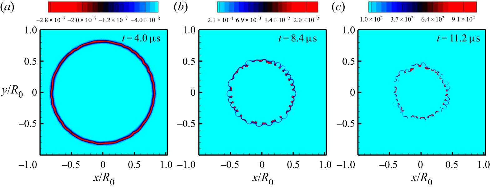
The contour slices of the consumption and production rates at three different instants are exhibited in figure 11. For the same instant, the contour slices of the consumption and production rates are similar, and we just show one of them at different instants for the sake of simplicity. The heat release is associated with the consumption and production rates, and their spatial distributions before and around the instant of the first reshock in figure 11(a,b) are similar to the results in figure 9. However, their spatial distributions are different around the instant of the second reshock with a high degree of turbulent mixing. According to the definition of heat release, the discrepancy originates from the spatial discrepancy of temperature fields.
Contour slices of the consumption rate of oxygen (a) at  $t=4.0\,\mathrm {\mu }{\rm s}$, the consumption rate of hydrogen (b) at
 $t=8.4\,\mathrm {\mu }{\rm s}$ and the production rate of water (c) at
 $t=11.6\,\mathrm {\mu }{\rm s}$.

3.5. Turbulent statistics
In this section we carry out turbulent statistics of RMI with and without chemical reactions, especially focusing on the temporal evolution after reshock. The chemical reaction effects are reflected by some characteristic parameters, such as turbulent kinetic energy, enstrophy, helicity, viscous dissipation rate, palinstrophy, skewness, flatness, spectra and inter-scale fluxes.
3.5.1. Turbulent kinetic energy
To include the variable-density effects, the Favre-averaged technique is used to obtain the mean field as (Gatski & Bonnet Reference Gatski and Bonnet2013)
 \begin{equation} \tilde{u}_i=\frac{\overline{\rho u_i}}{\bar{\rho}}, \end{equation}
where  $\bar {\cdot }$ denotes the spatial average within mixing regions, and the fluctuating component is defined as
 $u''_i=u_i-\tilde {u}_i$. In figure 12 we show the root mean square (r.m.s.) of radial, axial and circumferential velocity with and without chemical reactions over time to present the temporal developments of the anisotropy of the velocity field under the influence of a chemical reaction. The radial direction is dominant because of shock propagation. After reshock, the fluctuating development rate of radial velocity is smaller with a chemical reaction than that without a chemical reaction. In the late stage, the decay rates of all velocity components with a chemical reaction are faster because of larger viscous dissipation with heat release. The axial and circumferential directions are homogeneous, and their differences without a chemical reaction in figure 12(b) are negligible, especially in the late time. However, the differences of axial and circumferential components with a chemical reaction are apparent. This indicates that a chemical reaction hinders the anisotropy recovery process, which is different from classic decaying homogeneous and isotropic turbulence.
(a) The r.m.s. of radial velocity with and without chemical reactions over time. (b) The r.m.s. of axial and circumferential velocity with and without chemical reactions over time.

The turbulent kinetic energy is defined as
 \begin{equation} TKE=\frac{1}{2}\overline{\rho u''^2}. \end{equation}
According to the theoretical prediction of decaying homogeneous and isotropic turbulence, there exists a power-law solution of turbulent kinetic energy as  $TKE \sim t^{-\theta }$ (Samtaney, Pullin & Kosovié Reference Samtaney, Pullin and Kosovié2001). The value
 $\theta =1$, based on the Kármán–Howarth similarity theory (Kármán & Howarth Reference Kármán and Howarth1938). There are also other predictions, such as
 $\theta =10/7$ based on the constancy of the Loitsianskii invariant,
 $\theta =6/5$ based on assuming a constant Saffman invariant (Saffman Reference Saffman1967), and
 $\theta =3/2$ based on the two-point longitudinal velocity correlation (Huang & Leonard Reference Huang and Leonard1994). Although Reynolds number dependence exists, the decay rates in RMI are always faster than those in classic homogeneous and isotropic turbulence (Groom & Thornber Reference Groom and Thornber2019, Reference Groom and Thornber2021). We computed the turbulent kinetic energy within the mixing regions and showed them in figure 13. We fitted the two numerical results in figure 13 and obtained the decaying exponent
 $\theta =2.05$ without a chemical reaction and
 $\theta =2.50$ with a chemical reaction. These two decay exponents are relatively large, which may originate from the relatively low Reynolds number in the present numerical simulations. Under the influence of chemical reactions, the decay rate of turbulent kinetic energy is larger, which is also attributed to larger viscous dissipation with chemical reactions.
The turbulent kinetic energy with and without chemical reactions over time.

3.5.2. Mixed mass
The mixed mass can be regarded as a direct marker of the mixing regions, which is very important for experimental measurements (Zhou, Cabot & Thornber Reference Zhou, Cabot and Thornber2016; Zhang et al. Reference Zhang, Ruan, Xie and Tian2020; Zhou et al. Reference Zhou, Groom and Thornber2020; Bender et al. Reference Bender2021). Because of the appearance of nitrogen, we need to deal with the case of three-species mixing. Hence, we extend the definition of the mixed mass for two-species diffusion to the case of three-species diffusion as
 \begin{equation} \varPhi=\int 27 \rho Y_1 Y_2 Y_3 \,{\rm d}V, \end{equation}
where  $Y_1$,
 $Y_2$ and
 $Y_3$ are the mass fractions, and
 $Y_1+Y_2+Y_3$=1. The coefficient 27 is introduced to assure that the mixed mass is
 $\int \rho dV$ if the three mass fractions are equal, and it is similar to the consideration of the coefficient for the two-species diffusion (Zhang et al. Reference Zhang, Ruan, Xie and Tian2020). After a simple deduction based on the mass equation (2.1a) and species equation (2.1d), we can obtain the governing equation of the mixed mass as
 \begin{align} \frac{{\rm d}}{{\rm d}t}\int 27 \rho Y_1 Y_2 Y_3 \,{\rm d}V =27\int \rho D_m \frac{\partial Y_m}{\partial x_j}\frac{\partial \left( Y_n Y_l\right)}{\partial x_j}\,{\rm d}V,\quad (m,n,l=1,2,3, m\neq n \neq l). \end{align}
The above governing equation indicates that the newly defined mixed mass is also a conserved quantity, and its temporal evolution originates from the diffusion process. In order to evaluate the mixed mass at the initial time, we adopt the hyperbolic tangent function present in (2.12) to determine the mass fraction distributions. The hydrogen is placed inside the perturbed interface for the current configurations, and the oxygen is placed outside the perturbed interface. The nitrogen distributes inside and outside the perturbed interface with different volume fractions. The species distributions along the radial direction are shown schematically in figure 14. We assume that the density involved in the definition of the mixed mass does not affect the boundedness, and we focus on the remaining part. The distributions of mass fractions are expressed as
 \begin{equation} Y_{1}=\frac{1-c2}{2}\left[1+\tanh(r)\right],Y_{2}=\frac{c2-c1}{2}\left[1+\tanh(r)\right]+c1, Y_{3}=1-Y_{1}-Y_{2}, \end{equation}
where  $c1$ denotes the mass fraction of nitrogen within the perturbed interface and
 $c2$ denotes the mass fraction of nitrogen without the perturbed interface. The remaining part can be computed as
 \begin{equation} \int_{-\infty}^{+\infty} Y_{1} Y_{2} Y_{3} \,{\rm d}r=\frac{\left(c1+c2\right)\left(1-c1\right)\left(1-c2\right)}{4}. \end{equation}
The boundedness of the mixed mass in the initial time indicates that the expression (3.7) might be appropriate. In addition, the boundedness of the expression (3.7) can also be proven through the error function distribution of the involved species.
The schematic configuration of the three-species distributions with hyperbolic tangent function. The  $c1$ and
 $c2$ denote the mass fractions of nitrogen inside and outside the perturbed interface, respectively.

Correspondingly, the normalized mixed mass can be defined as
 \begin{equation} \varPsi=\frac{\int\rho Y_1 Y_2 Y_3 \,{\rm d}V}{\int \bar{\rho} \bar{Y}_1 \bar{Y}_2 \bar{Y}_3 \,{\rm d}V}. \end{equation}
The normalized mixed mass measures the mixing degree within the mixing regions, and it corresponds to 1 for the completely mixed fluid and 0 for the complete segregation, respectively. Here, the subscript  $1,2$ and
 $3$ may correspond to oxygen, nitrogen and hydrogen, respectively.
The differences of the mixed masses and normalized mixed masses with and without chemical reactions are shown in figure 15, and the mixed masses and normalized mixed masses with and without chemical reactions are shown in the inset of figure 15. We select the initial mass within the perturbed interface to normalize the mixed mass. The mixed masses with and without chemical reactions are approximately up to 2 % of the initial mass within the perturbed interface, and the difference of the mixed masses is approximately up to 0.2 %. The tendency of the normalized mixed mass is consistent with the results of classical mixed mass for two-species diffusion (Zhou et al. Reference Zhou, Cabot and Thornber2016), and the asymptotic value is approximately 0.6. The slight difference with the results in Zhou et al. (Reference Zhou, Cabot and Thornber2016) might originate from the effects of shock strength, Atwood number, convergence, etc. Both the mixed mass and normalized mixed mass results indicate that the chemical reaction leads to a weak mixing, although it leads to faster growth of the mixing width. The weak mixing also originates from the heat release effect of the chemical reaction.
(a) The difference of the mixed masses with and without chemical reactions over time. The inset shows the mixed masses with and without chemical reactions over time. (b) The difference of the normalized mixed masses with and without chemical reactions over time. The inset shows the normalized mixed masses with and without chemical reactions over time.

3.5.3. Enstrophy and helicity
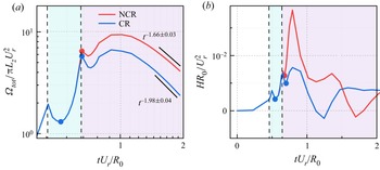
The enstrophy and helicity within the mixing regions are defined as
 \begin{equation} \varOmega_{tot}=\int_{V}\overline{\left(\frac{\omega_i \omega_i}{\rho}\right)} \,{\rm d}V, \quad H=\overline{u_i \omega_i}. \end{equation}
The enstrophy is used to feature the strength of vorticity, and the helicity reflects the broken degree of symmetry (Moffatt & Tsinober Reference Moffatt and Tsinober1992; Yan et al. Reference Yan, Li, Yu, Wang and Chen2020b). We show them with and without chemical reactions over time in figure 16. For enstrophy, chemical reactions hinder its development after reshock, and the decay rate is also larger than that without chemical reactions. Later, we fit the two numerical results and obtained decay rate  $\theta =1.66$ without a chemical reaction and
 $\theta =1.98$ with a chemical reaction, which are larger than the numerical consequence in planar geometry with
 $\theta =1.4$ (Zhou et al. Reference Zhou, Groom and Thornber2020). The discrepancy originates from the low-Reynolds-number effect in the present numerical simulations. The numerical results in figure 16(b) indicate the development of helicity, especially after reshock, along with turbulence development, and it might be marked as the transition or development of turbulence. In RMI with cylindrical geometry, the flows develop from quasi-two dimensions into three dimensions. The mathematical property of helicity can capture the transition process. In the late stage the changes of helicity are not monotonous, which might be attributed to chirality transfer along with viscous dissipation (Yan et al. Reference Yan, Li, Yu and Wang2020a). Because of chemical reactions, the helicity developments after reshock are hindered, and they correspond to weaker fluctuations.
Enstrophy (a) and helicity (b) with and without chemical reactions over time.

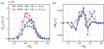
The radial distributions of enstrophy and helicity within the mixing regions at two characteristic instants marked in figure 16 are shown in figure 17. The first instant at  $t=12\,\mathrm {\mu }{\rm s}$ corresponds to the later development of perturbed interfaces compressed by reshock, and the second instant
 $t=13.2\,\mathrm {\mu }{\rm s}$ corresponds to the developed peak of the perturbed interfaces after reshock. With time passing, the developed enstrophy is mainly reflected as outer layers of mixing regions. The possible reason is that multiple reflected shock waves propagate between the centre and mixing regions, and the enstrophy is strengthened through baroclinic vorticity induced by multiple shock waves. The chemical reaction mainly occurs around the outer radius because of the full mixing of fuel and oxygen. The combustion wave propagates towards both the centre and outer regions, and the combustion wave represented as a high-pressure gradient leads to a higher baroclinic vorticity (Attal & Ramaprabhu Reference Attal and Ramaprabhu2015), which promotes the development of enstrophy in the outer layers of the mixing regions. For helicity along with radial distribution, the multiple shock wave and combustion wave effects are similar to those of enstrophy, especially around the outer layers of mixing with a chemical reaction. The radial distribution of helicity might not be regular in contrast to enstrophy, which reflects the complexity of helicity, and this will be further explored in the future.
Distribution of enstrophy (a) and helicity (b) with and without chemical reactions along the radial direction at  $t=12\,\mathrm {\mu }{\rm s}$ and
 $t=13.2\,\mathrm {\mu }{\rm s}$.

3.5.4. Palinstrophy
To explore the viscous dissipation mechanism of enstrophy, we derive the averaged governing equations of enstrophy in compressible flows as
 \begin{equation} \frac{{\rm d}}{{\rm d}t}\overline{\left( \omega_i \omega_i \right)}=\overline{\omega_i \omega_j \frac{\partial u_i}{\partial x_j}}-2\overline{\omega_i \omega_i \frac{\partial u_k}{\partial x_k}}+\overline{\frac{2}{\rho^2}\varepsilon_{ijk}\omega_i\frac{\partial \rho}{\partial x_j}\frac{\partial p}{\partial x_k}}+\overline{2\varepsilon_{ijk}\omega_i \frac{\partial}{\partial x_j}\left(\frac{1}{\rho}\frac{\partial \sigma_{lk}}{\partial x_l}\right)}. \end{equation}
In the incompressible limit the viscous term can be rewritten as  $-2\nu P(t)$, and
 $P(t)$ is the palinstrophy defined as
 \begin{equation} P(t)=\frac{1}{2}\overline{\left( \boldsymbol{\nabla} \times \omega \right)^2}=\int_0^{+\infty}k^4 E(k,t)\,{\rm d}k, \end{equation}
where  $k=|\boldsymbol {k}|$,
 $\boldsymbol {k}$ is the wavenumber and
 $E(k,t)$ is the energy spectrum density (Lesieur Reference Lesieur1997). The palinstrophy highlights the small-scale structures and the tightening of vorticity contours (Gauthier Reference Gauthier2017), and it is related to the skewness factor for isotropic turbulence (Batchelor & Townsend Reference Batchelor and Townsend1947). In two-dimensional turbulent flows the palinstrophy increases with enstrophy cascading to larger wavenumbers (Pouquet et al. Reference Pouquet, Lesieur, André and Basdevant1975; Tran & Dritschel Reference Tran and Dritschel2006).
In compressible flows, if we assume the kinematic viscosity coefficient is a constant, the viscous term of (3.13) is the same as that in incompressible flows. This means that the viscous dissipation of enstrophy in three-dimensional compressible flows does not concern compressibility, and the theoretical achievements in incompressible flows also apply to compressible flows.
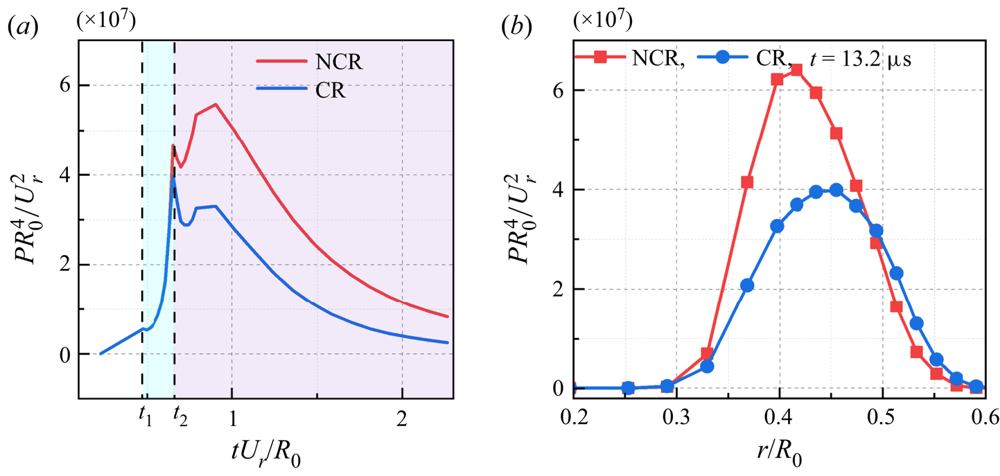
In figure 18 we show the palinstrophy averaged within mixing regions over time and the radial distribution at  $t=13.2 \,\mathrm {\mu }{\rm s}$. The development of palinstrophy is behind enstrophy and after reshock because different time scales exist for enstrophy and palinstrophy. The amplitude of the palinstrophy with a chemical reaction is smaller than that without a chemical reaction, and it originates from a higher viscosity coefficient of the heat release effect. The smaller the scales, the more apparent the role of viscosity. Hence, the palinstrophy reflecting small scales is damped by higher viscosity. The damping effect of a chemical reaction is also reflected on the radial distributions of palinstrophy in figure 18(b), especially on the inner and centre mixing regions. Around outer regions, the palinstrophy with a chemical reaction is slightly larger, which also results from the high-pressure gradient because of combustion waves. The outer mixing region with a chemical reaction is underdeveloped, and the baroclinic vorticity promotes small-scale developments.
(a) Palinstrophy with and without chemical reactions over time. (b) The distribution of palinstrophy along the radial direction at  $t=13.2\,\mathrm {\mu }{\rm s}$.

3.5.5. Skewness and flatness
For any random variable  $X$, the skewness and flatness are defined as
 \begin{equation} S=\frac{\langle X^3 \rangle}{\langle X^2 \rangle ^{3/2}}, \quad F=\frac{\langle X^4 \rangle}{\langle X^2 \rangle ^2}. \end{equation}
The skewness measures the asymmetry of probability distribution functions (p.d.f.s), and the flatness measures the discrepancy degree from a Gaussian distribution (Sahoo, Bonaccorso & Biferale Reference Sahoo, Bonaccorso and Biferale2015).
Orszag (Reference Orszag1977) proposed that for decaying isotropic turbulent flows, the relation of skewness of velocity gradient and palinstrophy is
 \begin{equation} S(t)=2.35\frac{\nu P(t)}{\left(\omega_i \omega_i\right)^{3/2}}. \end{equation}
Although this identity relation is no longer valid in the present three-dimensional RMI with and without chemical reactions, it also reflects the relationship of skewness and palinstrophy, and both of them highlight the small scales.
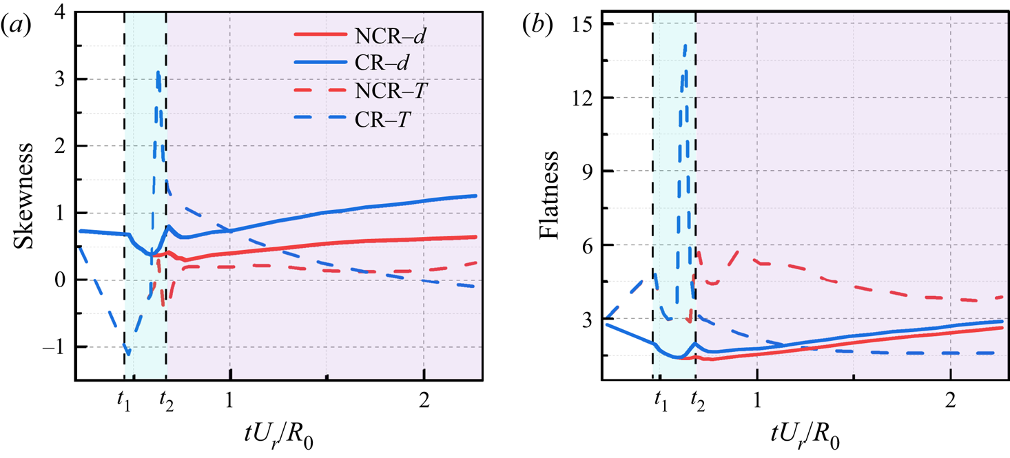
In figure 19 we show the skewness and flatness of velocities in the radial and circumferential directions. The statistical results of velocity in the axial direction are similar to those in the circumferential direction, and we do not show them for the sake of simplicity. For the velocity skewness, the radial velocity skewness is larger than that in the circumferential or axial directions. Because the radial direction is dominant, it corresponds to a larger asymmetry of radial velocity. In the early stage after reshock, the skewness increases monotonically during the shock compression process on the perturbed interface and during the development process. When the skewness is large enough, the role of multiple weaker shock compressions is apparent. The damping effects of the chemical reaction are reflected in the smaller skewness of velocity. The flatness of the dominant radial velocity in figure 19(b) is smaller, which indicates that the higher-order moments affected by the main shock wave are not fully developed. In contrast, the higher-order moments of circumferential velocity can eliminate the constraint effects of radial direction mixing, and small scales can be developed more fully. In the late time the flatness with a chemical reaction is larger, and it corresponds to a more intermittent status. Hence, a larger flatness means a larger discrepancy from the Gaussian distribution, and a smaller skewness means a weaker asymmetry with the chemical reaction.
The skewness (a) and flatness (b) of radial  $u_r$ and circumferential
 $u_\theta$ velocity with and without chemical reactions over time.

In addition, we compute the skewness and flatness of the mixture density and temperature with and without chemical reactions in figure 20. Before reshock, the discrepancies of skewness and flatness with and without chemical reactions are negligible. For the density field, a chemical reaction involves more element mixing, and the skewness and flatness are larger than those without a chemical reaction. For the temperature field, at the early stage after reshock, the skewness and flatness are larger because of heat release effects, especially around the outer layer of mixing regions. As time passes, the discrepancy degree of skewness with and without chemical reactions decreases. With fuller mixing of fuel and oxygen after reshock, the chemical reaction apparently begins to occur, and the combustion wave propagates towards two sides. At the early stage of a chemical reaction, the temperature varies dramatically, leading to larger skewness and flatness. The temperature gradient decreases with the propagation of combustion waves, and the skewness and flatness also decrease. In the late time the temperature field becomes smoother with higher viscosity and results in smaller skewness and flatness. The higher-order moment is more sensitive to the propagating combustion waves.
Skewness (a) and flatness (b) of mixture density and temperature with and without chemical reactions over time.

3.5.6. Viscous dissipation rate
The ensemble-averaged enstrophy is associated with viscous dissipation (Yeung, Zhai & Sreenivasan Reference Yeung, Zhai and Sreenivasan2015), and we rewrite the ensemble-averaged enstrophy in compressible flows as
 \begin{equation} \left\langle \omega^2 \right\rangle=\frac{1}{2}\left\langle \left( \frac{\partial u_i}{\partial x_j}-\frac{\partial u_j}{\partial x_i} \right) \left( \frac{\partial u_i}{\partial x_j}-\frac{\partial u_j}{\partial x_i} \right)\right\rangle=\left\langle \frac{\partial u_i}{\partial x_j}\frac{\partial u_i}{\partial x_j} \right\rangle-\left\langle \frac{\partial u_i}{\partial x_j}\frac{\partial u_j}{\partial x_i} \right\rangle. \end{equation}
The ensemble-averaged viscous dissipation rate  $\epsilon$ reads as
 \begin{equation} \epsilon=\left\langle \sigma_{ij}\frac{\partial u_i}{\partial x_j} \right\rangle=\left\langle\mu\left(\frac{\partial u_i}{\partial x_j}+\frac{\partial u_j}{\partial x_i}-\frac{2}{3}\theta\delta_{ij}\right)\cdot\frac{\partial u_i}{\partial x_j}\right\rangle. \end{equation}
Hence, if we assume the dynamic viscosity coefficient  $\mu$ to be a constant in total flow fields, we can obtain the following relation:
 \begin{equation} \epsilon=\bar{\mu}\langle \omega^2 \rangle+\frac{4}{3}\bar{\mu}\langle\theta^2\rangle+2\bar{\mu}\left\langle \frac{\partial}{\partial x_k}\left[ \frac{\left( u_k u_l \right)}{\partial x_l}-2 u_k \theta \right] \right\rangle. \end{equation}
Here  $\bar {\mu }$ is a mean dynamic viscosity coefficient defined by
 $\bar {\mu }=\langle \mu \rangle$, and the fluctuating dynamic viscosity coefficient is
 $\mu ^{\prime }=\mu -\bar {\mu }$.
However, the dynamic viscosity coefficient  $\mu$ fluctuates dramatically along with the temperature field. We show contour slices of the dynamic viscosity coefficient
 $\mu$ with and without chemical reactions at
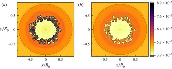
 $t=13.2\,\mathrm {\mu }{\rm s}$ in figure 21. Compared with the case without a chemical reaction, the dynamic viscosity coefficient with a chemical reaction fluctuates more dramatically, especially around the mixing regions because of heat release effects. Hence, the averaged dynamic viscosity coefficient cannot be used to exactly predict the total viscous dissipation rate. The viscous dissipation rate with a chemical reaction should be investigated through coupling the dynamic viscosity coefficient, enstrophy and velocity divergence. This coupling effect highlights the discrepancy of viscous dissipation rates between incompressible and compressible turbulence, in addition to the pressure-work defect (Eyink & Drivas Reference Eyink and Drivas2018).
Two-dimensional contour slices of dynamic viscosity coefficient  $\mu$ with a chemical reaction (a) and without a chemical reaction (b) at
 $t=13.2\,\mathrm {\mu }{\rm s}$.

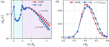
The averaged viscous dissipation rate within the mixing regions with and without chemical reactions over time and their distributions along the radial direction are shown in figure 22. The evolution of viscous dissipation rates is consistent with turbulent kinetic energy under the influence of multiple shock compression. After reshock, the viscous dissipation rate decreases due to shock compression and develops after the shock propagates out from the mixing regions. The viscous dissipation rate decays self-similarly in the late stage. The decaying exponents obtained by fitting are 2.14 and 2.53 without a chemical reaction and with a chemical reaction, respectively. The viscous dissipation rates with chemical reactions are smaller than those without chemical reactions, even though the dynamic viscous coefficient with chemical reactions is larger. The main reason is that the velocity gradient with a chemical reaction is smaller, which is also reflected in the smaller enstrophy and palinstrophy. The radial distributions of the viscous dissipation rates in figure 22(b) reveal that the smaller velocity gradients mainly work around the mixing centre, and the larger dynamic viscosity coefficients mainly work around the outer layers with an apparent chemical reaction.
(a) Viscous dissipation rates with and without chemical reactions over time. (b) The distribution of viscous dissipations along the radial direction at  $t=13.2\,\mathrm {\mu }{\rm s}$.

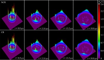
To visually investigate the spatial distributions of the viscous dissipation rates with and without chemical reactions, we show the three-dimensional surface diagrams of the viscous dissipation rates at some typical instants after reshock in figure 23. Because of the large velocity gradient across the shock, the viscous dissipation rates around the shock are dominant out of mixing regions. The spatial distributions of the viscous dissipation rates within the mixing regions are non-uniform, with many so-called extreme events (Yeung et al. Reference Yeung, Zhai and Sreenivasan2015; Debue et al. Reference Debue, Valori, Cuvier, Daviaud, Foucaut, Laval, Wiertel, Padilla and Dubrulle2021; Moffatt Reference Moffatt2021). These local extreme viscous dissipation rates within the mixing regions are similar to fully developed turbulent flows, and they also decay with time. Compared with the case without a chemical reaction at the same instant, the mixing regions with a chemical reaction present more intermittent structures of viscous dissipation rates, and the discrepancies around the propagating shock are negligible.
Three-dimensional surface diagrams of viscous dissipation rates with and without chemical reactions at some typical instants.

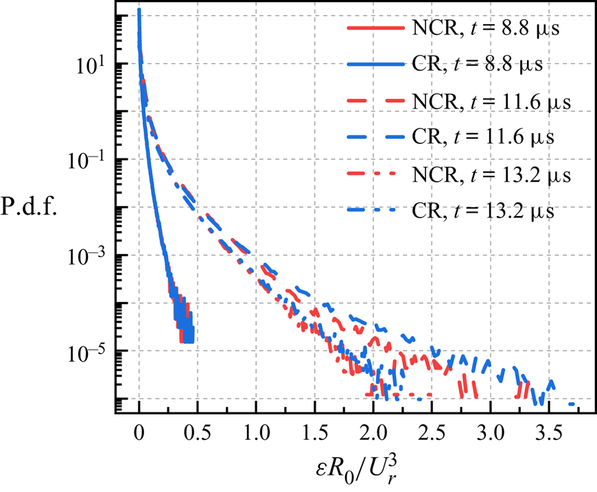
The chemical reaction effects on the spatial distributions of the viscous dissipation rates are further explored by the p.d.f.s in figure 24. We select some typical instants at  $t=8.8\,\mathrm {\mu }{\rm s}$ with the early time of shock compression, at
 $t=11.6 \,\mathrm {\mu }{\rm s}$ with the late time of shock compression, and at
 $t=13.2 \,\mathrm {\mu }{\rm s}$ with development getting rid of shock compression. At
 $t=8.8\,\mathrm {\mu }{\rm s}$, their discrepancies are negligible because the chemical reaction is not apparent at this instant. Later, at
 $t=11.6 \,\mathrm {\mu }{\rm s}$ with an apparent chemical reaction, the probabilities of higher fluctuations with a chemical reaction are larger, featured by the higher tail of its p.d.f. At
 $t=13.2 \,\mathrm {\mu }{\rm s}$, the highly fluctuating events decay, and even the fluctuations with chemical reactions are still larger than those without chemical reactions. The chemical reaction effects on the p.d.f.s are consistent with the conclusions in figure 23.
Probability distribution functions of the viscous dissipation rates with and without chemical reactions at  $t=8.8\,\mathrm {\mu }{\rm s}$,
 $t=11.6\,\mathrm {\mu }{\rm s}$ and
 $t=13.2\,\mathrm {\mu }{\rm s}$.

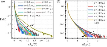
The evolutions of extreme events during shock compression and free development are investigated by the p.d.f.s without a chemical reaction in figure 25. The evolutions with chemical reactions are similar, and we do not show them for the sake of simplicity. During shock compression, although the averaged viscous dissipation rates are suppressed, the probabilities of extreme events increase, as represented by increasingly higher p.d.f. tails. After shock compression, the probabilities of extreme events begin to decay. Hence, extreme events develop along with shock compression. The main reason is that the shock is located within the mixing regions, and the large velocity gradients around the shock lead to higher viscous dissipation rates. With shock propagating towards the outer side, the extreme events of the viscous dissipation rates become more developed. Later, the extreme events begin to decay without shock located within the mixing regions. The largest fluctuations at different instants are approximately 100 orders of magnitude for the mean values, and these extreme events reveal the intrinsic intermittency of turbulent flows (Yeung et al. Reference Yeung, Zhai and Sreenivasan2015).
(a) Probability distribution functions of the viscous dissipation rates without a chemical reaction during shock compression. (b) Probability distribution functions of the viscous dissipation rates without a chemical reaction after shock compression.

3.5.7. Spectra and fluxes
To investigate the scale separations within the mixing regions, we study the spectra of velocity, density and temperature in this section. According to previous analyses of compressible turbulent flows, all of them obey the same power-law solutions with  $k^{-5/3}$ in the inertial subrange (Wang, Gotoh & Watanabe Reference Wang, Gotoh and Watanabe2017a; Wang et al. Reference Wang, Wan, Chen, Xie, Wang and Chen2019; Teng et al. Reference Teng, Wang, Li and Chen2020). The existence of the inertial subrange with a power-law solution is characteristic of fully developed turbulence (Zhou Reference Zhou2001).
The density and temperature spectra are dependent on circumferential wavenumbers at  $t=12\,\mathrm {\mu }{\rm s}$ during shock compression, at
 $t=13.2\,\mathrm {\mu }{\rm s}$ for free development and at
 $t=30\,\mathrm {\mu }{\rm s}$ at the late time are exhibited in figure 26. They obey the relation
 $\int _0^{\infty }E_X(k_{\theta })\,{\rm d} k_{\theta } =\langle X^{\prime 2}\rangle$,
 $E_X(k_{\theta })=\int _0^{\infty }\int _0^{\infty } \widehat {X^{\prime }}(k_r,k_{\theta },k_z)\widehat {X^{\prime }}^{*}(k_r,k_{\theta },k_z)\,{\rm d}k_r\, {\rm d}k_z$. Here,
 $\prime$ denotes the fluctuating component,
 $*$ denotes the complex conjugate,
 $\hat {\cdot }$ denotes the Fourier coefficient, and
 $X$ denotes
 $\rho$ for mixture density and
 $T$ for temperature. For mixture density spectra, the increase in spectral density at high wavenumbers and the decrease in spectral density at low wavenumbers from
 $t=12\,\mathrm {\mu }{\rm s}$ to
 $t=13.2\,\mathrm {\mu }{\rm s}$ mean that large-scale density cascades to small scales during free development, and then the mixture density spectra begin to decay at all scales. In the late stage the
 $-5/3$ scaling regions across half a decade are present. Because of the low Reynolds numbers in the present numerical simulations, the inertial subrange with uniform scaling may be short, but the present numerical results also confirm its existence. The chemical reaction effects on the density spectra are represented by high mixture density spectra at high wavenumbers, and this phenomenon is consistent with previous extreme events. For temperature spectra, the development regularity at the early stage is similar to mixture density spectra. Because of the heat release of chemical reactions, the temperature spectra with chemical reactions at low wavenumbers increase with time, and the temperature spectra at high wavenumbers begin to decay after free development. This means that the non-premixed chemical reaction within the mixing regions provides large-scale heat sources to inject internal energy into the flow field and temperature cascades from large scales to small scales. These temperature transfer routines are similar to forced homogeneous and isotropic turbulence (Wang et al. Reference Wang, Wan, Chen, Xie, Wang and Chen2019; Yan et al. Reference Yan, Li, Yu and Wang2020a,Reference Yan, Li, Yu, Wang and Chenb), and the inertial subrange with a
 $-5/3$ scaling over one decade begins to appear in the present numerical simulations. However, the temperature spectra without a chemical reaction would decrease at all scales after free development.
The spectra of fluctuating mixture density (a) and temperature (b) with and without chemical reactions at  $t=12\,\mathrm {\mu }{\rm s}$,
 $t=13.2\,\mathrm {\mu }{\rm s}$ and
 $t=30\,\mathrm {\mu }{\rm s}$.

Zhou (Reference Zhou2001) proposed that the scaling exponent of kinetic energy should be  $-3/2$ for RMI, although the discrepancy from the classic Kolmogorov scaling
 $-5/3$ is small (Groom & Thornber Reference Groom and Thornber2019). We select the same instants of mixture density and temperature to explore the scale separation of radial and axial velocities in figure 27, and their definitions are consistent with density and temperature spectra with
 $X=u_r$ and
 $X=u_z$. For radial and axial velocity spectra, inertial subranges are not apparent because of low Reynolds numbers, and their spectra with chemical reactions are small because of higher viscous dissipation rates within the mixing regions at early times. During free development of radial velocity, small scales could not be developed because the radial developments of velocity are constrained by multi-species mixing. This circumstance would be changed for axial velocity with periodic boundary conditions, and small scales can be developed to some extent and then begin to decay.
The spectra of fluctuating radial (a) and axial velocity (b) with and without chemical reactions at  $t=12\,\mathrm {\mu }{\rm s}$,
 $t=13.2\,\mathrm {\mu }{\rm s}$ and
 $t=30\,\mathrm {\mu }{\rm s}$.

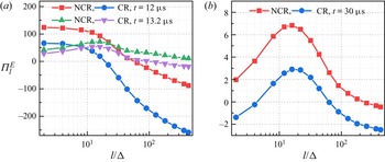
The inter-scale transfer process of kinetic energy reveals the complexity of compressible turbulent flows, and a filter operation can be employed as a mathematical tool to study the kinetic energy cascade (Wang et al. Reference Wang, Yang, Shi, Xiao, He and Chen2013a; Zhao, Liu & Lu Reference Zhao, Liu and Lu2020). We only focus on the inter-scale kinetic energy transfer and rewrite the kinetic energy flux term as
 \begin{equation} \varPi_l^E={-}\bar{\rho}\left( \widetilde{\boldsymbol{u}\boldsymbol{u}}-\tilde{\boldsymbol{u}}\tilde{\boldsymbol{u}} \right):\boldsymbol{\nabla} \tilde{\boldsymbol{u}}, \end{equation}
where  $\tilde {\boldsymbol {u}}$ is the Favre-filtered velocity defined as
 $\tilde {\boldsymbol {u}}=\bar {\rho \boldsymbol {u}}/\bar {\rho }$. In figure 28 we select three typical instants at
 $t=12\,\mathrm {\mu }{\rm s}$,
 $t=13.2\,\mathrm {\mu }{\rm s}$ and
 $t=30\,\mathrm {\mu }{\rm s}$ to explore the kinetic energy cascade across axial scales. During shock compression at
 $t=12\,\mathrm {\mu }{\rm s}$, the kinetic energy fluxes at moderate and large scales are negative, which means kinetic energy cascades inversely from small scales to large scales. This phenomenon is consistent with constraint fluctuations during shock compression. The shock compression effects can be explained as kinetic energy transferring from small scales into large scales, and it is more apparent with a chemical reaction. During free development, the backward energy cascade would not be dominant, and there exists a net forward energy cascade from large scales to small scales. In the late time the amplitudes of the kinetic energy cascade decrease, which reflects a weakened nonlinear interaction. The ensemble averages of kinetic energy fluxes with chemical reactions are always smaller than those without chemical reactions, which indicates two intrinsic mechanisms of the chemical reaction. The first is that the chemical reaction weakens the nonlinear interactions with heat release, leading to smaller energy fluxes. The second might be that chemical reactions promote kinetic energy transfer inversely to large scales (Teng et al. Reference Teng, Wang, Li and Chen2021).
(a) The ensemble averages of kinetic energy flux at  $t=12\,\mathrm {\mu }{\rm s}$ and
 $t=13.2\,\mathrm {\mu }{\rm s}$. (b) The ensemble averages of kinetic energy flux at
 $t=30\,\mathrm {\mu }{\rm s}$. Here
 $l$ is the filter width, and
 $\varDelta$ is the grid spacing.

4. Conclusions
The reactive RMI is widely present in the engineering flows, and evolution characteristics of the flow field are different from that without a chemical reaction (Zhou et al. Reference Zhou2021). There exists important progress in the past few years, and most of them focus on the planar geometry, two-dimensional numerical simulations or single-step chemical kinetic mechanisms (Attal & Ramaprabhu Reference Attal and Ramaprabhu2015; Attal et al. Reference Attal, Ramaprabhu, Hossain, Karkhanis, Uddin, Gord and Royd2015; Bambauer et al. Reference Bambauer, Hasslberger and Klein2020, Reference Bambauer, Chakraborty, Klein and Hasslberger2021). The regulations should be extended to some practical applications, and we carry out three-dimensional DNS with multi-mode perturbations and a detailed chemical mechanism of the cylindrical geometry in this paper. For the element chemical reaction of non-premixed hydrogen and oxygen, 9-species and 19-reaction models are adopted. The chemical reaction effects on the process of transition and late-time turbulent mixing are highlighted to uncover the temporal evolution of RMI with heat release and combustion wave propagation. The complex interactions of shock and chemical reaction lead to a quick growth of the mixing width and weakened turbulent mixing. They are reflected on different positions within the mixing regions, which means that the combustion wave promotes the boundary development of the mixing regions and heat release weakens the turbulent mixing around the centre of the mixing regions. With time after the second reshock, the turbulent mixing would decay and the chemical reaction would be dominant in the late stage. Hence, the eventual mixing is suppressed by the chemical reaction.
To study the process of transition and turbulent mixing, we employ multi-mode initial interfacial perturbation. Our numerical results reveal that the similarity exponent of shock propagation is consistent with theoretical prediction, the Taylor Reynolds number is large enough for fully developed turbulent flows, and the grid resolution is small enough to capture the Kolmogorov viscous length scales. All of these results assure the reliable accuracy of the present numerical simulations.
We proposed a new definition of mixing width for more-species chemical reactions, which involved all elements of all species. The evolutions of the inner radius of mixing regions with and without chemical reactions are nearly the same, while the outer radii are different. Because of non-premixed combustion and combustion wave propagation, the growth rate of the outer radial with a chemical reaction is larger. The heat release results in a larger temperature gradient around the outer radius, and it promotes the growth of the mixing width.
Sufficient energy is needed for the occurrence of the chemical reaction, and it absorbs energy from the flow field in the early times. Nevertheless, the total internal energy within the mixing regions increases over time. The main reason lies in the fact that the change of the internal energy induced by the propagating shock wave is much larger than that induced by the chemical reaction, under the present thermodynamic conditions. After reshock, the fuller mixing of fuels and oxygen leads to a drastic chemical reaction, and their discrepancies in the mixing characteristics and turbulent statistics begin to be apparent. The fuller chemical reaction is reflected in the large heat release rate, large production and consumption rate. Because of the smaller scales of spike distribution, the chemical reaction occurs mainly within the mixing regions, and tends to happen towards the spikes. The highlighted statistical variables within the mixing regions mainly include turbulent kinetic energy, enstrophy, helicity, viscous dissipation rate, palinstrophy, skewness, flatness, spectra and inter-scale fluxes. Because of the heat release of the chemical reaction, the fluctuating radial velocity is smaller, and the corresponding decay rate is larger in the late time. After reshock, the enstrophy and helicity begin to develop gradually, while chemical reactions hinder the development process. The development of helicity after reshock might be regarded as the transition mark in the present three-dimensional cylindrical RMI because the strong three-dimensional instability comes from quasi-two-dimensional perturbations. The palinstrophy is related to the viscous dissipation of enstrophy and skewness, and we can prove that compressibility does not affect the viscous dissipation of enstrophy in compressible flows. The developments of small-scale structures with chemical reactions after reshock are weakened, but the high-order moments are fully developed later by removing the main shock wave.
The above physical process descriptions can be attributed to the multiple shock effects locally, and the physical regulations obtained in the cylindrical geometry is similar to that in the planar geometry. We carried out DNS of RMI with reshock and a chemical reaction in the planar geometry, and the numerical setting is consistent with the shock tube facility at Los Alamos National Laboratory (Balakumar et al. Reference Balakumar, Orlicz, Tomkins and Prestridge2008; Orlicz et al. Reference Orlicz, Balakumar, Tomkins and Prestridge2009; Balakumar et al. Reference Balakumar, Orlicz, Ristorcelli, Balasubramanian, Prestridge and Tomkins2012; Tomkins et al. Reference Tomkins, Kumar, Orlicz and Prestridge2008, Reference Tomkins, Balakumar, Orlicz, Prestridge and Ristorcelli2013) in the Appendix A. The accelerated growth of the mixing width induced by the generated combustion wave is varied after the reshock and before the rarefaction wave. The weakened turbulent mixing is validated by the larger decaying rate of turbulent kinetic energy before reshock. More specific details have been given in the Appendix A.
We compare the spectra and inter-scale fluxes with and without chemical reactions to differ their multiscale characteristics. After reshock, the spectral densities at high wavenumbers begin to develop and then decay. While the spectral densities at low wavenumbers decay over time. Hence, there exists a time range of the developments of small-scale structures. The spectra of thermal variables, such as density and temperature, show apparent inertial subranges, while the inertial subranges of velocity spectra are not apparent because of the low Reynolds number in the present numerical simulations. The amplitudes of the multiscale distributions of velocity fields with chemical reactions are smaller than those without chemical reactions. For the temperature spectra, the amplitudes with chemical reactions are larger because of heat release. The shock compression corresponds to an inverse energy cascade, which is strengthened by a chemical reaction. Then, the amplitudes of kinetic energy fluxes with chemical reactions are always smaller than those without chemical reactions, which reflects the weakened nonlinear interactions and promotes the process of the inverse energy cascade.
To summarize, we perform three-dimensional DNS of cylindrical RMI with and without chemical reactions and uncover the chemical reaction effects on the transition and late-time turbulent mixing. The growth of the mixing width is promoted by the chemical reaction because of combustion wave propagation, and turbulent mixing is weakened by the chemical reaction because of heat release.
Acknowledgements
The authors thank the National Supercomputer Center in Tianjin (NSCC-TJ) and National Supercomputer Center in GuangZhou (NSCC-GZ) for providing computer time. In addition, we would like to express our honest appreciation to Professor D.L. Youngs and Professor B. Thornber for their generosity in providing the code of the initial perturbations in the planar geometry, and Professor Y. Zhang and Dr C. Zhang for many useful discussions.
Funding
This work was supported by the National Key Research and Development Program of China (2019YFA0405300 and 2020YFA0711800), the National Natural Science Foundation of China (NSFC grant no. 12072349 and no. 91852203), and the Strategic Priority Research Program of Chinese Academy of Science (grant, NO.XDPB25).
Declaration of interests
The authors report no conflict of interest.
Appendix A. DNS of RMI with a chemical reaction in a planar geometry
We carry out DNS of RMI with a chemical reaction in a planar geometry to illustrate the chemical reaction effect on the mixing transition and turbulent statistics. The initial configurations are exhibited schematically in figure 29. The cross-section length is 20 mm, and the streamwise length is 137 mm, which is consistent with the shock tube facility at Los Alamos National Laboratory (Balakumar et al. Reference Balakumar, Orlicz, Tomkins and Prestridge2008; Orlicz et al. Reference Orlicz, Balakumar, Tomkins and Prestridge2009; Tomkins et al. Reference Tomkins, Kumar, Orlicz and Prestridge2008, Reference Tomkins, Balakumar, Orlicz, Prestridge and Ristorcelli2013; Balakumar et al. Reference Balakumar, Orlicz, Ristorcelli, Balasubramanian, Prestridge and Tomkins2012). The initial perturbed interface centre locates at  $x=0$ m, and the initial shock wave locates at
 $x=0.005$ m. To avoid the reflected shock effect, we adopt a buffer region adjoint to the left main computational domain with a stretched grid. The amplitude of the initial perturbed interface is determined by a power spectrum method (Thornber et al. Reference Thornber, Drikakis, Youngs and Williams2010, Reference Thornber2017), and it can be expressed as
 $$\begin{align} A(y, z)&= \sum_{m, n=0}^{N} a_{m, n} \cos \left(k_{0} m y\right) \cos \left(k_{0} n z\right) +b_{m, n} \cos \left(k_{0} m y\right) \sin \left(k_{0} n z\right)\nonumber\\ &\quad +c_{m, n} \sin \left(k_{0} m y\right) \cos \left(k_{0} n z\right) +d_{m, n} \sin \left(k_{0} m y\right) \sin \left(k_{0} n z\right), \end{align}$$
where  $k_0=2{\rm \pi} /L$,
 $L$ is the length of the cross-section, and
 $m$ and
 $n$ are the perturbed modes in the
 $y$ and
 $z$ directions, respectively. Other details refer to a previous valuable paper (Thornber et al. Reference Thornber2017). In our numerical simulations the perturbed mode ranges from 8 to 32, and 256 grid cells are used in the cross-section. According to our previous conclusion, the heat released by the chemical reaction decreases the needed grid number to resolve the Kolmogorov scale. Other initial parameter settings are listed in table 2.
The initial computational configurations of the planar geometry.

Initial parameter settings of the planar geometry.

The determination method of the bubble and spike positions of the planar geometry is consistent with that of the cylindrical geometry. To be mentioned, we adopt a plane-averaged approach to obtain the mean physical variable  $\langle a(x) \rangle$ as
 \begin{align} \left\langle a(x) \right\rangle =\frac{1}{\iint \,{{\rm d} y} \,{\rm d}z}\iint a(x,y,z) \,{{\rm d} y}\,{\rm d}z. \end{align}
We show the displacement of the bubbles, spikes and shock wave in figure 30(a). From the beginning, the shock wave propagates along the streamwise direction, and then interacts with the perturbed interface for the first time. A rarefaction wave is generated and propagates in an opposite direction. In the meantime, a transmitted shock wave propagates in the streamwise direction until the right rigid wall. The shocked perturbed interface would move along the streamwise direction, and interact with the reshock subsequently. The mixing width evolutions are shown in figure 30(b), the growth of the mixing width after the reshock is linear, and it is consistent with the linear reshock model (Mikaelian Reference Mikaelian1989). After the linear growth of the mixing width, we found that the mixing width is re-accelerated, and it may originate from the promoting effect of the generated combustion wave.
(a) Displacement of the bubbles, spikes and shock wave of the planar geometry. (b) The mixing width over time of the planar geometry.

We show the ratio of the Kolmogorov scale and grid spacing over time in figure 31(a), and the ratios are larger than 0.5 except around the times with shock and reshock. The shock itself leads to a large velocity gradient, and may induce additional viscosity dissipation. Hence, the current grid resolution is sufficient to obtain the following highlighted parameters. In figure 31(b) we show the turbulent kinetic energy over time. Every shock corresponds to a huge increase of turbulent kinetic energy. Before the reshock, the turbulent kinetic energy decays self-similarly with a decay exponent  $\theta \approx 1.17$. After the reshock, the decay rate is larger. The larger decay rate may partly originate from the apparent chemical reaction after the reshock. Because of the limit of the shock tube length, the reflected shock wave after the first reshock would interact with the perturbed interface repeatedly. In contrast to the cylindrical geometry without any wall, the development of the perturbed interface is affected by multiple shocks, and the self-similar decay exponent is hard to obtain.
(a) The ratio of the Kolmogorov scale and grid spacing over time of the planar geometry. (b) The turbulent kinetic energy of the planar geometry.

The directional Taylor Reynolds numbers are shown in figure 32(a). All directional Taylor Reynolds numbers are larger than 100–140, and they satisfy the transition criteria (Dimotakis Reference Dimotakis2000; Zhou et al. Reference Zhou, Clark, Clark, Glendinning, Skinner, Huntington, Hurricane, Dimits and Remington2019). The temporal evolution of the directional Taylor Reynolds numbers is similar to that in the shock tube facility (Balakumar et al. Reference Balakumar, Orlicz, Tomkins and Prestridge2008; Orlicz et al. Reference Orlicz, Balakumar, Tomkins and Prestridge2009; Balakumar et al. Reference Balakumar, Orlicz, Ristorcelli, Balasubramanian, Prestridge and Tomkins2012). However, they are larger than that of the cylindrical geometry. The main reason may lie in a larger Taylor microscale of the planar geometry. The discrepancy may also originate from the initial perturbations, the convergent geometry effect, etc. The enstrophy evolution in figure 32(b) is similar to the trend of the directional Taylor Reynolds numbers.
(a) Taylor Reynolds numbers over time of the planar geometry. (b) The enstrophy over time of the planar geometry.