1 Introduction
The tokamak is characterized by a strong axisymmetric toroidal magnetic field and a relatively weak poloidal field, in the geometry of a large aspect ratio toroid. Given this, scale lengths perpendicular to the magnetic field
 $\boldsymbol{B}$
are shorter than along
 $\boldsymbol{B}$
, resulting in a disparate separation of fundamental MHD mode frequencies. In particular, the magnetosonic mode is at higher frequency and separates from the shear Alfvén wave with a frequency ratio of
 $O(\unicode[STIX]{x1D716})$
, where
 $\unicode[STIX]{x1D716}$
is the inverse aspect ratio. This separation allows a reduction of the ideal MHD equations (White et al.
Reference White, Monticello, Rosenbluth, Strauss and Kadomtsev1974; Strauss Reference Strauss1976, Reference Strauss1977) wherein the reduced system describes shear Alfvén waves and is quasi-static with respect to the magnetosonic modes. Another MHD frequency of interest in tokamaks is that of sound waves. For a typical low beta system like a tokamak, this frequency is below the Alfvén frequency by the square root of
 $\unicode[STIX]{x1D6FD}$
, the ratio of thermal energy to magnetic energy. The sound frequency band is generally also of the same order as the frequency of drift waves and of interchange-like modes (which incorporate Mercier modes and geodesic acoustic modes).
This paper is concerned with a reduction of the MHD equations to frequencies at the sonic level; in particular, frequencies of interest are below the ballooning Alfvén frequency,
 $c_{A}/qR$
. At sub-Alfvénic frequencies, any MHD convection in the system must be consistent with interchanges of magnetic field lines that, to lowest order, preserve the magnetic structure. The frequencies of interest that can then be studied include sound waves (
 $c_{s}/qR$
), Mercier interchange modes
 $(c_{s}/R)(a/L_{n})$
, geodesic acoustic modes (GAMs) (
 $c_{s}/R$
), drift waves (
 $c_{s}\unicode[STIX]{x1D70C}_{i}/(aL_{n})$
) and zonal flows (zero frequency). Here,
 $c_{A}$
,
 $c_{s}$
,
 $a$
,
 $R$
,
 $L_{n}$
,
 $\unicode[STIX]{x1D70C}_{i}$
and
 $q$
are, respectively, the Alfvén speed, sound speed, minor radius, major radius, density scale length, ion Larmor radius and the safety factor. An expansion in
 $\unicode[STIX]{x1D716}\sim a/R$
is made.
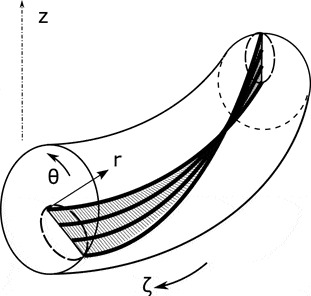
To lowest order, the dominant motions are electrostatic convection cells in the cross-field plane as shown pictorially in figure 1. Thus, to lowest order, the expansion is centred about and in the vicinity of a low-order rational surface; in particular, the off-rational part of the magnetic pitch and the magnetic shear are considered weaker than the poloidal magnetic field. In our expansion, these weaker portions are allowed in higher order, thus allowing magnetic shear. We clarify later in the paper what restrictions these assumptions put on our system of equations. We allow wavelengths long compared to the gyroradius but comparable to the size of the tokamak. With the inclusion of resistivity, tearing modes, resistive ballooning modes, Pfirsch–Schluter cells and the Stringer spin-up are also included. Since the system is largely electrostatic, the magnetic field acts as a ‘guide’ to the convection and, therefore, a major advantage of the reduction is that the resulting system of nonlinear equations is two-dimensional.
Interchanges on a rational flux surface.

In what follows, we systematically derive, starting from the full ideal MHD equations, reduced equations at sonic frequencies. Since the frequency of interest is two orders below the magnetosonic frequency, we find we have to go to
 $O(\unicode[STIX]{x1D716}^{4})$
to obtain a closed set of equations. Consequently, the required algebra is tedious and several cancellations of terms are found. As a check on the algebra, we find it helpful to motivate the cancellations by proceeding to the eikonal (WKB) limit and comparing with the expected local dispersions based on previous work.
In § 2, we outline the ordering of the full MHD equations and systematically derive reduced equations in a periodic cylinder. We begin with a cylinder as it serves to establish the basic methodology and allows us to introduce the notation, etc. In § 3, then, we extend this to a torus. This brings in toroidal curvature effects and, in particular, introduces new variables, with harmonic content, to the system. In § 4, we show that the toroidal equations of § 3 can be greatly simplified by a redefinition of variables: with the redefinition, two cancellations, motivated by examining WKB limits, are demonstrated and the resulting system is then rendered physically more transparent.
A rationale for reduction of toroidal MHD equations to the sonic level has been articulated by Waelbroeck (Reference Waelbroeck2011). A primary interest is that a reduction to this level allows drift waves and the associated small-scale turbulent transport. While we do not include drift waves in this paper, for simplicity, the ordering and methodology, in principle, should allow this band of frequencies for wavelengths longer than the ion gyroradius. While the ordering and methodology does allow drift waves, the actual implementation remains to be shown. The ideal Reduced MHD (RMHD) equations were previously generalized and extended self-consistently to the resistive MHD case by Drake and Antonsen (DA) (Drake & Antonsen Jr Reference Drake and Antonsen1984). They pointed out that earlier attempts by Schmalz (Reference Schmalz1981), Izzo et al. (Reference Izzo, Monticello, Park, Manickam, Strauss, Grimm and McGuire1983) and Strauss (Reference Strauss1983) to obtain resistive modes in a large aspect ratio tokamak by simply retaining higher powers of
 $\unicode[STIX]{x1D716}$
was not self-consistent. This is because the sub-Alfvénic modes are sensitive to magnetic geometry and a more careful asymptotic analysis is required. The sensitivity of magnetic geometry can be seen from the fact that the magnetic fields in this limit behave like ‘stiff’ rods and the sub-Alfvénic modes would have to quasi-statically adjust themselves to avoid bending the field lines. In this paper, we present a systematic expansion up to fourth-order in
 $\unicode[STIX]{x1D716}$
.
2 Sub-Alfvénic reduced MHD in a cylinder
We begin our reduction of equations for the case of a straight cylinder; this establishes the ordering and methodology. We employ standard
 $(r,\unicode[STIX]{x1D703},\unicode[STIX]{x1D701})$
cylindrical geometry with the unit vector
 $\hat{\unicode[STIX]{x1D73B}}$
in the direction of the symmetry direction of the cylinder. We assume a periodic cylinder of radius
 $a$
and axial length
 $2\unicode[STIX]{x03C0}R$
.
2.1 Equations and ordering
We begin with the ideal MHD equations:
 $$\begin{eqnarray}\displaystyle & \unicode[STIX]{x2202}_{t}n+\unicode[STIX]{x1D735}\boldsymbol{\cdot }(n\boldsymbol{u})=0 & \displaystyle\end{eqnarray}$$
 $$\begin{eqnarray}\displaystyle & M_{i}n(\unicode[STIX]{x2202}_{t}+\boldsymbol{u}\boldsymbol{\cdot }\unicode[STIX]{x1D735})\boldsymbol{u}=-\unicode[STIX]{x1D735}p+\boldsymbol{j}\times \boldsymbol{B},\quad \unicode[STIX]{x1D707}_{0}\,\boldsymbol{j}\equiv \unicode[STIX]{x1D735}\times \boldsymbol{B} & \displaystyle\end{eqnarray}$$
 $$\begin{eqnarray}\displaystyle & \unicode[STIX]{x2202}_{t}\boldsymbol{B}=-\unicode[STIX]{x1D735}\times \boldsymbol{E} & \displaystyle\end{eqnarray}$$
 $$\begin{eqnarray}\displaystyle & \unicode[STIX]{x1D735}\boldsymbol{\cdot }\boldsymbol{B}=0. & \displaystyle\end{eqnarray}$$
Standard notation is used. We have
 $M_{i}$
as the ion mass,
 $n$
as the density,
 $\boldsymbol{u}$
as the flow,
 $\unicode[STIX]{x1D707}_{0}$
as the permeability of free space,
 $\boldsymbol{j}$
as the current,
 $\boldsymbol{E}$
and
 $\boldsymbol{B}$
as the electric and magnetic fields, and pressure
 $p=nT$
with
 $T=T_{e}+T_{i}$
. We assume constant isothermal temperature
 $T$
, for simplicity. For ideal MHD,
 $$\begin{eqnarray}\boldsymbol{E}=-\boldsymbol{u}\times \boldsymbol{B}.\end{eqnarray}$$
This forms a complete set for the variables
 $\{n,\boldsymbol{U},\boldsymbol{B}\}$
. We shall use both
 $\boldsymbol{U}$
and
 $\boldsymbol{u}$
, interchangeably, to represent the flow vector. In this section, it is more convenient to use
 $\boldsymbol{B}\equiv \unicode[STIX]{x1D735}\times \boldsymbol{A}$
. This results in
 $$\begin{eqnarray}\unicode[STIX]{x2202}_{t}\boldsymbol{A}=-\boldsymbol{E}-\unicode[STIX]{x1D735}\unicode[STIX]{x1D711}.\end{eqnarray}$$
Equation (2.6) replaces (2.3) and (2.4). Thus, the primary equations are (2.1), (2.2), (2.6).
For the asymptotic expansion, we adopt the following ordering:
 $$\begin{eqnarray}\frac{k_{\Vert }}{k_{\bot }}\sim \frac{|\boldsymbol{u}_{\bot }|}{c_{s}}\sim \frac{U_{\Vert }}{c_{s}}\sim \frac{B_{\unicode[STIX]{x1D703}}}{B_{\unicode[STIX]{x1D701}}}\sim \frac{c_{s}}{c_{A}}\sim \sqrt{\unicode[STIX]{x1D6FD}}\sim \unicode[STIX]{x1D716},\end{eqnarray}$$
where
 $k_{\Vert }$
,
 $k_{\bot }$
are the wavenumbers parallel and perpendicular to the full magnetic field
 $\boldsymbol{B}$
, with poloidal and toroidal components
 $B_{\unicode[STIX]{x1D703}}$
and
 $B_{\unicode[STIX]{x1D701}}$
,
 $c_{s}$
is the sound speed
 $\equiv (T/M)^{1/2}$
and
 $\unicode[STIX]{x1D6FD}=nT/(B^{2}/2\unicode[STIX]{x1D707}_{0})$
. The primary expansion parameter is
 $\unicode[STIX]{x1D716}\sim a/R\ll 1$
. We assume
 $q\sim O(1)$
and it follows
 $B_{\unicode[STIX]{x1D703}}/B_{\unicode[STIX]{x1D701}}\sim \unicode[STIX]{x1D716}$
. For optimal ordering, we choose
 $c_{s}/c_{A}\sim \unicode[STIX]{x1D716}$
. The primary mode of interest is the quasi-static interchange mode, or Mercier mode, whose frequency is
 $c_{s}/R$
; thus
 $\unicode[STIX]{x1D714}\sim c_{s}/R\sim O(\unicode[STIX]{x1D716}^{2})$
. Nonlinearly, we expect
 $\unicode[STIX]{x2202}_{t}\sim \boldsymbol{u}_{\bot }\boldsymbol{\cdot }\unicode[STIX]{x1D735}$
and thus,
 $|\boldsymbol{u}_{\bot }|\sim \unicode[STIX]{x1D716}c_{s}$
. Finally, we also expect
 $\unicode[STIX]{x1D735}\boldsymbol{\cdot }\boldsymbol{u}$
to be small or order unity; now
 $\unicode[STIX]{x1D735}\boldsymbol{\cdot }\boldsymbol{u}_{\bot }$
is non-zero only if
 $\unicode[STIX]{x1D716}\neq 0$
, since
 $|\boldsymbol{B}|$
is almost constant. Thus,
 $\unicode[STIX]{x1D735}\boldsymbol{\cdot }\boldsymbol{u}_{\bot }\sim \unicode[STIX]{x1D716}|\boldsymbol{u}_{\bot }|/a$
from which, using
 $\unicode[STIX]{x1D735}\boldsymbol{\cdot }\boldsymbol{u}\approx 0$
, we get
 $U_{\Vert }\sim \unicode[STIX]{x1D716}c_{s}\sim \unicode[STIX]{x1D716}^{2}$
. The last ansatz is discussed in more detail in appendix E.
Since in the large aspect ratio limit the lowest-order magnetic field is toroidal, it is more convenient to define parallel and perpendicular with respect to the toroidal axis. With this ordering, we find that the terms in the
 $n$
and
 $\boldsymbol{A}$
equations, equations (2.1), (2.6), each are of the same order. However, the momentum equation is ordered as
 $$\begin{eqnarray}\left.\begin{array}{@{}c@{}}M_{i}n(\unicode[STIX]{x2202}_{t}+\boldsymbol{u}\boldsymbol{\cdot }\unicode[STIX]{x1D735})\boldsymbol{u}=-\unicode[STIX]{x1D735}p+\boldsymbol{j}\times \boldsymbol{B}\\ \unicode[STIX]{x1D716}^{4}\quad :\quad \unicode[STIX]{x1D716}^{4}\quad :\quad \unicode[STIX]{x1D6FD}\sim \unicode[STIX]{x1D716}^{2}\quad :\quad 1.\quad \end{array}\right\}\end{eqnarray}$$
Thus, we would need to go to at least fourth order to close the system. To systematically apply the asymptotic expansion, we will need annihilation equations for the momentum equations. These are:
 $$\begin{eqnarray}\displaystyle & \displaystyle \boldsymbol{B}\boldsymbol{\cdot }\left(M_{i}n\frac{\text{d}\boldsymbol{U}}{\text{d}t}+\unicode[STIX]{x1D735}p\right)=0 & \displaystyle\end{eqnarray}$$
 $$\begin{eqnarray}\displaystyle & \displaystyle \unicode[STIX]{x1D735}\boldsymbol{\cdot }\left(M_{i}n\frac{\text{d}\boldsymbol{U}}{\text{d}t}\times \frac{\hat{\boldsymbol{b}}}{B}\right)=\boldsymbol{B}\boldsymbol{\cdot }\unicode[STIX]{x1D735}\left(\frac{j_{\Vert }}{B}\right)+\frac{1}{B^{2}}\,\boldsymbol{j}\boldsymbol{\cdot }\unicode[STIX]{x1D735}p+2\hat{\boldsymbol{b}}\times \unicode[STIX]{x1D735}p\boldsymbol{\cdot }\unicode[STIX]{x1D735}\left(\frac{1}{B}\right). & \displaystyle\end{eqnarray}$$
We will also find useful as an annihilator the parallel component of the
 $\boldsymbol{A}$
equation, namely
 $$\begin{eqnarray}\boldsymbol{B}\boldsymbol{\cdot }\unicode[STIX]{x2202}_{t}\boldsymbol{A}=-\boldsymbol{B}\boldsymbol{\cdot }\unicode[STIX]{x1D735}\unicode[STIX]{x1D711}.\end{eqnarray}$$
This corresponds to the
 $E_{\Vert }=0$
condition of ideal MHD.
In what follows we assume that the magnetic field is predominantly axial along a cylindrical axis (i.e. in the
 $\hat{\unicode[STIX]{x1D73B}}$
direction). All quantities designated as
 $\bot$
will be assumed to be perpendicular to
 $\hat{\unicode[STIX]{x1D73B}}$
(not
 $\boldsymbol{B}$
, as is often the convention). In this case, it will be convenient to assume the form
 $$\begin{eqnarray}\boldsymbol{B}=I\unicode[STIX]{x1D735}\unicode[STIX]{x1D701}+\boldsymbol{B}_{\bot },\end{eqnarray}$$
where
 $I\equiv RB_{\unicode[STIX]{x1D701}}$
is the toroidal current.
2.2 Asymptotic expansion of the ideal MHD equations
We now proceed order by order systematically. The momentum equation starts at zero order, while all the other equations (density, Faradays law and the consistency conditions) start at second order. Normalization parameters used are the minor radius, Alfvén speed and magnetic field:
 $\{a,c_{A},B_{0}\}$
respectively. These parameters will simply be set to unity. We do a perturbative expansion in the large aspect ratio parameter
 $\unicode[STIX]{x1D716}\ll 1$
according to:
 $$\begin{eqnarray}\left.\begin{array}{@{}c@{}}\boldsymbol{B}=\boldsymbol{B}_{0}+\unicode[STIX]{x1D716}\boldsymbol{B}_{1}+\cdots ,\quad \unicode[STIX]{x1D713}=\unicode[STIX]{x1D713}_{0}+\unicode[STIX]{x1D716}\unicode[STIX]{x1D713}_{1}+\cdots \\ I=I_{-1}/\unicode[STIX]{x1D716}+I_{0}+\unicode[STIX]{x1D716}I_{1}+\cdots ,\quad \boldsymbol{j}=\boldsymbol{j}_{\mathbf{0}}+\unicode[STIX]{x1D716}\boldsymbol{j}_{\mathbf{1}}+\cdots \\ R=1/\unicode[STIX]{x1D716},\quad \boldsymbol{B}\boldsymbol{\cdot }\unicode[STIX]{x1D735}=\unicode[STIX]{x1D716}(\boldsymbol{B}\boldsymbol{\cdot }\unicode[STIX]{x1D735})_{1}+\unicode[STIX]{x1D716}^{2}(\boldsymbol{B}\boldsymbol{\cdot }\unicode[STIX]{x1D735})_{2}+\cdots ,\\ \text{d}/\text{d}t=\unicode[STIX]{x1D716}^{2}d_{t},\quad \unicode[STIX]{x1D711}=\unicode[STIX]{x1D716}^{2}\unicode[STIX]{x1D711}_{2}+\unicode[STIX]{x1D716}^{3}\unicode[STIX]{x1D711}_{3}+\cdots ,\quad U_{\Vert }=\unicode[STIX]{x1D716}^{2}U_{\Vert 2}+\cdots \\ n=n_{0}+\unicode[STIX]{x1D716}n_{1}+\cdots ,\quad \unicode[STIX]{x1D6FD}\equiv \unicode[STIX]{x1D716}^{2}\bar{\unicode[STIX]{x1D6FD}},\quad p=\unicode[STIX]{x1D716}^{2}n\bar{\unicode[STIX]{x1D6FD}},\quad \unicode[STIX]{x1D702}\equiv \unicode[STIX]{x1D716}^{2}\bar{\unicode[STIX]{x1D702}},\quad {\hat{s}}\equiv \unicode[STIX]{x1D716}\bar{s},\end{array}\right\}\end{eqnarray}$$
where
 ${\hat{s}}$
is the magnetic shear and the magnetic flux
 $\unicode[STIX]{x1D713}$
will be introduced below in (2.17). We have defined the quantities
 $\bar{\unicode[STIX]{x1D6FD}},\bar{\unicode[STIX]{x1D702}}$
so that these are
 $O(1)$
quantities as opposed to
 $\unicode[STIX]{x1D6FD},\unicode[STIX]{x1D702}$
etc.
To lowest order,
 $O(\unicode[STIX]{x1D716}^{0})$
:
 $$\begin{eqnarray}\boldsymbol{j}_{0}\times \boldsymbol{B}_{\mathbf{0}}=0,\quad \boldsymbol{j}_{0}\equiv \unicode[STIX]{x1D735}_{\bot }\times \boldsymbol{B}_{\mathbf{0}}.\end{eqnarray}$$
We assume that the magnetic field is purely axial to lowest order and thus
 $\boldsymbol{B}_{0}=\hat{\unicode[STIX]{x1D73B}}$
, and
 $\boldsymbol{j}_{0}=0$
. From (2.12) we see that
 $$\begin{eqnarray}\boldsymbol{B}_{0}=\hat{\unicode[STIX]{x1D73B}},\quad I_{-1}=1,\end{eqnarray}$$
where we use
 $R=1/\unicode[STIX]{x1D716}$
. To
 $O(\unicode[STIX]{x1D716}^{1})$
, we obtain
 $$\begin{eqnarray}\boldsymbol{j}_{1}\times \hat{\unicode[STIX]{x1D73B}}=0\quad \Rightarrow \quad \boldsymbol{j}_{1}=J_{1}\hat{\unicode[STIX]{x1D73B}}.\end{eqnarray}$$
Now, from (2.2),
 $\boldsymbol{j}_{1}=\unicode[STIX]{x1D735}_{\bot }\times \boldsymbol{B}_{\bot \mathbf{1}}+\unicode[STIX]{x1D735}I_{0}\times \hat{\unicode[STIX]{x1D73B}}$
. To first order, we also have
 $\unicode[STIX]{x1D735}\boldsymbol{\cdot }\boldsymbol{B}_{\bot \mathbf{1}}=0$
which implies
 $\boldsymbol{B}_{\bot \mathbf{1}}=\hat{\unicode[STIX]{x1D73B}}\times \unicode[STIX]{x1D735}\unicode[STIX]{x1D713}_{0}$
. Using these and condition (2.16) above, we get
 $I_{0}=\text{const.}$
and
 $$\begin{eqnarray}\boldsymbol{B}_{1}=\hat{\unicode[STIX]{x1D73B}}\times \unicode[STIX]{x1D735}\unicode[STIX]{x1D713}_{0},\quad J_{1}=\unicode[STIX]{x1D6FB}_{\bot }^{2}\unicode[STIX]{x1D713}_{0}.\end{eqnarray}$$
We further make the choice, for the predominantly axial geometry we are considering, that
 $I_{0}=0$
.
Field line following coordinate system.

We now proceed to
 $O(\unicode[STIX]{x1D716}^{2})$
. We first have the annihilation (2.10), which is second order at the lowest significant order. The only term that contributes at this order is the ‘field line bending term’
 $\boldsymbol{B}\boldsymbol{\cdot }\unicode[STIX]{x1D735}(\,j_{\Vert }/B)$
; the other terms enter, at a minimum, at fourth order, given that
 $I_{0}$
is zero. This results in
 $$\begin{eqnarray}(\boldsymbol{B}\boldsymbol{\cdot }\unicode[STIX]{x1D735})_{1}(\,j_{\Vert }/B)_{1}=0\quad \Rightarrow \quad (\,j_{\Vert }/B)_{1}=J_{1}(r)=\unicode[STIX]{x1D6FB}_{\bot }^{2}\unicode[STIX]{x1D713}_{0}.\end{eqnarray}$$
The magnetic field at this order involves a constant axial field,
 $B_{0}=1$
and an azimuthal field
 $\hat{\unicode[STIX]{x1D73B}}\times \unicode[STIX]{x1D735}\unicode[STIX]{x1D713}_{0}$
. We make the choice of a time independent
 $\unicode[STIX]{x1D713}_{0}(r)=r^{2}/(2q_{0})$
. This choice corresponds to a constant axial current
 $J_{1}=2/q_{0}$
and implies a helical net field with the same winding number on each radial surface. In particular, the well-known tokamak safety factor,
 $q(r)=rB_{\unicode[STIX]{x1D701}}/RB_{\unicode[STIX]{x1D703}}$
, is a constant,
 $q_{0}$
, and there is no magnetic shear. Additionally, we assume
 $q_{0}$
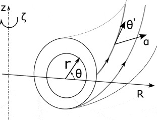
is rational, and so we define a helical coordinate system (see figure 2) with respect to the magnetic field given by the transformation
 $$\begin{eqnarray}r^{\prime }=r,\quad \unicode[STIX]{x1D703}^{\prime }=\unicode[STIX]{x1D703},\quad \unicode[STIX]{x1D6FC}=\unicode[STIX]{x1D703}-(1/q_{0})\unicode[STIX]{x1D701}.\end{eqnarray}$$
For the purposes of this paper, we will assume that the magnetic shear is small, in the sense that any shear will be included as a correction term at the level of
 $\unicode[STIX]{x1D713}_{1}$
. Likewise, we assume that any non-rational part of the magnetic field is also weak and enters at the
 $\unicode[STIX]{x1D713}_{1}$
order. We will discuss later how these assumptions, while self-consistent, constrain our equations to apply only within a certain radial domain. We note that
 $$\begin{eqnarray}(\boldsymbol{B}\boldsymbol{\cdot }\unicode[STIX]{x1D735})_{1}=(1/q_{0})\unicode[STIX]{x2202}_{\unicode[STIX]{x1D703}^{\prime }}\end{eqnarray}$$
in the helical coordinate system. In this field aligned coordinate system, as is clear from (2.19), there is a periodicity with respect to the variable
 $\unicode[STIX]{x1D703}^{\prime }$
, which is the poloidal angle
 $\unicode[STIX]{x1D703}$
holding the flux surface label
 $r$
and the field line label
 $\unicode[STIX]{x1D6FC}$
fixed on a given rational surface with
 $q_{0}=m/n$
(
 $m$
and
 $n$
integers). Thus the
 $(\boldsymbol{B}\boldsymbol{\cdot }\unicode[STIX]{x1D735})_{1}$
operator (2.20) can be annihilated by averaging over a closed field line. After a toroidal circuit,
 $\unicode[STIX]{x1D703}^{\prime }$
goes from
 $\unicode[STIX]{x1D6FC}$
to
 $\unicode[STIX]{x1D6FC}+2\unicode[STIX]{x03C0}/q_{0}$
and thus
 $$\begin{eqnarray}\oint \text{d}\unicode[STIX]{x1D703}^{\prime }(\boldsymbol{B}\boldsymbol{\cdot }\unicode[STIX]{x1D735})_{1}f=0,\quad \oint \text{d}\unicode[STIX]{x1D703}^{\prime }=2\unicode[STIX]{x03C0}/q_{0}.\end{eqnarray}$$
Continuing our expansion at second order, we get, in addition to (2.18),
 $$\begin{eqnarray}(\,\boldsymbol{j}\times \boldsymbol{B})_{2}=\boldsymbol{j}_{2}\times \hat{\unicode[STIX]{x1D73B}}+\boldsymbol{j}_{1}\times \boldsymbol{B}_{\bot \mathbf{1}}=\unicode[STIX]{x1D735}_{\bot }p_{2}=\bar{\unicode[STIX]{x1D6FD}}\unicode[STIX]{x1D735}_{\bot }n_{0}.\end{eqnarray}$$
Calculating
 $\boldsymbol{j}$
to second order using the form (2.12) for
 $\boldsymbol{B}$
, and noting that
 $\boldsymbol{B}_{\bot \mathbf{1}}$
is axisymmetric, we have
 $\boldsymbol{j}_{2}\times \hat{\unicode[STIX]{x1D73B}}=-\unicode[STIX]{x1D735}_{\bot }I_{1}$
. Using this in (2.22), we can integrate (2.22) with respect to the perpendicular coordinates to get
 $$\begin{eqnarray}\bar{\unicode[STIX]{x1D6FD}}n_{0}+I_{1}+\unicode[STIX]{x1D713}_{0}\unicode[STIX]{x1D6FB}_{\bot }^{2}\unicode[STIX]{x1D713}_{0}=0.\end{eqnarray}$$
This is the Grad–Shafranov equation. In our accounting, this is an equation for
 $I_{1}$
: note that since
 $n_{0}$
is not necessarily axisymmetric (we will describe this later),
 $I_{1}$
is also in general non-axisymmetric (as by implication is the axial magnetic field, to second order).
Next, we consider equation (2.6) taken to second order. The time derivative term is zero since
 $A_{\bot }^{(0)}$
is time independent, being proportional to
 $I_{-1}$
. Using (2.5), we then deduce from the right-hand side of (2.6) that
 $$\begin{eqnarray}\boldsymbol{u}_{2}=U_{\Vert 2}\hat{\unicode[STIX]{x1D73B}}+\hat{\unicode[STIX]{x1D73B}}\times \unicode[STIX]{x1D735}\unicode[STIX]{x1D711}_{2}.\end{eqnarray}$$
Finally, at the
 $O(\unicode[STIX]{x1D716}^{2})$
order, we have from (2.1)
 $$\begin{eqnarray}d_{t}n_{0}=0,\end{eqnarray}$$
where
 $d_{t}=\unicode[STIX]{x2202}_{t}+\hat{\unicode[STIX]{x1D73B}}\times \unicode[STIX]{x1D735}\unicode[STIX]{x1D711}_{2}\boldsymbol{\cdot }\unicode[STIX]{x1D735}$
. We note also that the condition
 $(\unicode[STIX]{x1D735}\boldsymbol{\cdot }\boldsymbol{B})_{2}=0$
becomes
 $\unicode[STIX]{x1D735}_{\bot }\boldsymbol{\cdot }\boldsymbol{B}_{\bot \mathbf{2}}=0$
, since
 $I_{0}=0$
. This implies that
 $\boldsymbol{B}_{\bot \mathbf{2}}$
can also be written in terms of the flux function
 $\unicode[STIX]{x1D713}$
, viz.,
 $$\begin{eqnarray}\boldsymbol{B}_{\bot \mathbf{2}}=\hat{\unicode[STIX]{x1D73B}}\times \unicode[STIX]{x1D735}\unicode[STIX]{x1D713}_{1}.\end{eqnarray}$$
We now proceed to
 $O(\unicode[STIX]{x1D716}^{3})$
. The annihilation equation (2.10) becomes
 $$\begin{eqnarray}(\boldsymbol{B}\boldsymbol{\cdot }\unicode[STIX]{x1D735})_{1}(j_{\Vert }/B)_{2}+(\boldsymbol{B}\boldsymbol{\cdot }\unicode[STIX]{x1D735})_{2}(j_{\Vert }/B)_{1}=0,\end{eqnarray}$$
where, again, we note that the remaining terms in the equation contribute only at fourth order. To calculate
 $\boldsymbol{j}\boldsymbol{\cdot }\boldsymbol{B}/B^{2}$
to second order, we note that
 $\boldsymbol{j}_{\bot }\boldsymbol{\cdot }\boldsymbol{B}_{\bot }$
is of order
 $\unicode[STIX]{x1D716}^{3}$
since
 $\boldsymbol{j}_{\bot }$
is of second order, at largest. Thus to the required order
 $$\begin{eqnarray}(\,j_{\Vert }/B)_{2}=(I\unicode[STIX]{x1D735}\unicode[STIX]{x1D701}\boldsymbol{\cdot }(\unicode[STIX]{x1D735}\times \boldsymbol{B})/B^{2})_{2}=\unicode[STIX]{x1D6FB}_{\bot }^{2}\unicode[STIX]{x1D713}_{1}.\end{eqnarray}$$
Using this in the expression for
 $j_{\Vert }/B$
above, we find the annihilation condition to be
 $$\begin{eqnarray}(\boldsymbol{B}\boldsymbol{\cdot }\unicode[STIX]{x1D735})_{1}\unicode[STIX]{x1D6FB}_{\bot }^{2}\unicode[STIX]{x1D713}_{1}=0.\end{eqnarray}$$
It is readily checked that the operator
 $(\boldsymbol{B}\boldsymbol{\cdot }\unicode[STIX]{x1D735})_{1}$
, from (2.20), commutes with the cylindrical Laplacian. Thus,
 $\unicode[STIX]{x1D713}_{1}$
is a ‘flute function’, that is to say it is constant along a twisted magnetic field line but not necessarily constant across the field lines, i.e.
 $\unicode[STIX]{x1D713}_{1}=\unicode[STIX]{x1D713}_{1}(r,\unicode[STIX]{x1D6FC})$
. From here on, we will suppress the prime on
 $r$
as there is no ambiguity. We also find, from the annihilation equation (2.9),
 $$\begin{eqnarray}(\boldsymbol{B}\boldsymbol{\cdot }\unicode[STIX]{x1D735})_{1}n_{0}=0.\end{eqnarray}$$
We now write (2.6) at third order. An as yet unknown term,
 $\boldsymbol{u}_{3}\times \hat{\unicode[STIX]{x1D73B}}$
, appears on the right-hand side and can be annihilated by dotting with
 $\hat{\unicode[STIX]{x1D73B}}$
(or, equivalently, using the annihilation equation (2.11)). Noting that
 $\unicode[STIX]{x1D716}\boldsymbol{A}_{1}=-\unicode[STIX]{x1D713}_{0}\unicode[STIX]{x1D735}\unicode[STIX]{x1D701}$
, consistent with (2.17), and that
 $\unicode[STIX]{x1D713}_{0}$
is self-consistently time independent, the annihilated equation becomes
 $$\begin{eqnarray}(\boldsymbol{B}\boldsymbol{\cdot }\unicode[STIX]{x1D735})_{1}\unicode[STIX]{x1D711}_{2}=0.\end{eqnarray}$$
The foregoing three equations imply that all of the functions
 $\{n_{0},\unicode[STIX]{x1D711}_{2},\unicode[STIX]{x1D713}_{1}\}$
are flute functions. We denote
 $\unicode[STIX]{x1D713}_{1}$
by
 $\text{}\underline{\unicode[STIX]{x1D713}_{1}}$
to emphasize its flute nature.
We pause here to collect the description for the
 $\boldsymbol{B}$
field so far.
 $\boldsymbol{B}$
is, in general written as (2.12). To the extent that we have obtained so far, to second order in
 $\unicode[STIX]{x1D716}$
, expressions for
 $I_{-1},I_{0}$
and
 $I_{1}$
, and expressions for
 $\unicode[STIX]{x1D713}_{0}$
and
 $\text{}\underline{\unicode[STIX]{x1D713}_{1}}$
, (see (2.15), (2.23), (2.26) and (2.29)), we may write the
 $B$
field from (2.12), in familiar form, as
 $$\begin{eqnarray}\boldsymbol{B}=I\unicode[STIX]{x1D735}\unicode[STIX]{x1D701}+\unicode[STIX]{x1D735}\unicode[STIX]{x1D701}\times \unicode[STIX]{x1D735}\unicode[STIX]{x1D713}+O(\unicode[STIX]{x1D716}^{3}),\end{eqnarray}$$
where
 $I=I_{-1}+I_{1}(r,\unicode[STIX]{x1D6FC})$
and
 $\unicode[STIX]{x1D713}=\unicode[STIX]{x1D713}_{0}(r)+\text{}\underline{\unicode[STIX]{x1D713}_{1}}(r,\unicode[STIX]{x1D6FC})$
. This expression for
 $\boldsymbol{B}$
is familiar; it is correct to second order in
 $\unicode[STIX]{x1D716}$
and only third-order terms are dropped. Note, however, that the field is not axisymmetric (usually the form (2.32) is employed for axisymmetric fields). We will show in what follows that this is the only required precision in
 $\boldsymbol{B}$
necessary to close our set of equations.
Finally, we go to fourth order. We first apply the
 $E_{\Vert }=0$
annihilation condition (2.11). This gives us
 $$\begin{eqnarray}(\boldsymbol{B}\boldsymbol{\cdot }\unicode[STIX]{x1D735})_{1}\unicode[STIX]{x1D711}_{3}+(\boldsymbol{B}\boldsymbol{\cdot }\unicode[STIX]{x1D735})_{2}\unicode[STIX]{x1D711}_{2}=\unicode[STIX]{x2202}\text{}\underline{\unicode[STIX]{x1D713}_{1}}/\unicode[STIX]{x2202}t.\end{eqnarray}$$
The
 $\unicode[STIX]{x1D711}_{3}$
term is higher order and not needed. This term can be annihilated by integrating over each separate closed field line for fixed
 $\unicode[STIX]{x1D6FC}$
, i.e. we use the condition
 $\oint \text{d}\unicode[STIX]{x1D703}^{\prime }(\boldsymbol{B}\boldsymbol{\cdot }\unicode[STIX]{x1D735})_{1}f=0$
. We get
 $$\begin{eqnarray}d_{t}\text{}\underline{\unicode[STIX]{x1D713}_{1}}=0.\end{eqnarray}$$
We now proceed to the annihilation equation (2.10). The field line bending term,
 $\boldsymbol{B}\boldsymbol{\cdot }\unicode[STIX]{x1D735}(j_{\Vert }/B)$
, is the largest term. This term, to fourth order, is
 $(\boldsymbol{B}\boldsymbol{\cdot }\unicode[STIX]{x1D735})_{1}(\,j_{\Vert }/B)_{3}+(\boldsymbol{B}\boldsymbol{\cdot }\unicode[STIX]{x1D735})_{2}(\,j_{\Vert }/B)_{2}$
, since
 $(\,j_{\Vert }/B)_{1}$
is a constant. As above, we annihilate the
 $(\,j_{\Vert }/B)_{3}$
term by field line averaging. The remaining terms yield the vorticity equation (see 2.10), viz.
 $$\begin{eqnarray}\unicode[STIX]{x1D735}_{\bot }\boldsymbol{\cdot }(d_{t}n_{0}\unicode[STIX]{x1D735}_{\bot }\unicode[STIX]{x1D711}_{2})=\frac{2\bar{\unicode[STIX]{x1D6FD}}}{q_{0}}\unicode[STIX]{x2202}_{\unicode[STIX]{x1D701}}n_{0}+(\boldsymbol{B}\boldsymbol{\cdot }\unicode[STIX]{x1D735})_{2}\unicode[STIX]{x1D6FB}_{\bot }^{2}\text{}\underline{\unicode[STIX]{x1D713}_{1}}.\end{eqnarray}$$
Here, the left-hand side, being the ‘smallest’ term, is calculated to lowest order in the cylindrical geometry. An expression for
 $(\,j_{\Vert }/B)_{2}$
was previously obtained (see (2.28)) and has been used to calculate the surviving field line bending term, where
 $(\boldsymbol{B}\boldsymbol{\cdot }\unicode[STIX]{x1D735})_{2}=\hat{\unicode[STIX]{x1D73B}}\times \unicode[STIX]{x1D735}\text{}\underline{\unicode[STIX]{x1D713}_{1}}\boldsymbol{\cdot }\unicode[STIX]{x1D735}$
. The
 $\boldsymbol{j}\boldsymbol{\cdot }\unicode[STIX]{x1D735}p=\boldsymbol{j}_{2}\boldsymbol{\cdot }\unicode[STIX]{x1D735}p_{2}$
term is zero because of the pressure balance condition, equation (2.22). The only non-zero contribution from the term proportional to
 $\boldsymbol{B}\times \unicode[STIX]{x1D735}p\boldsymbol{\cdot }\unicode[STIX]{x1D735}(1/B^{2})$
is
 $J_{1}\hat{\unicode[STIX]{x1D73B}}\times \unicode[STIX]{x1D735}\unicode[STIX]{x1D713}_{0}\boldsymbol{\cdot }\unicode[STIX]{x1D735}n_{0}$
on account that
 $I_{0}=0$
and that the non-constant part of
 $I_{1}$
is equal to
 $p_{2}$
, as seen from (2.23). Using (2.30), this term can be shown to give the first term on the right-hand side.
Equations (2.25), (2.34) and (2.35) now constitute a closed system for the flute functions
 $n_{0}$
,
 $\unicode[STIX]{x1D711}_{2}$
and
 $\text{}\underline{\unicode[STIX]{x1D713}_{1}}$
. These equations incorporate the cylindrical flute interchange, and also the shear Alfvén wave in the presence of weak magnetic shear (or weakly off-rational fields). Together, these describe the low
 $\unicode[STIX]{x1D6FD}$
interchange in a sheared field. Magnetic shear is introduced in the system in the
 $\text{}\underline{\unicode[STIX]{x1D713}_{1}}$
field as follows: the usual tokamak safety factor
 $q$
is defined as
 $1/q(r)=RB_{\unicode[STIX]{x1D703}}/(rB_{\unicode[STIX]{x1D701}})$
, where
 $B_{\unicode[STIX]{x1D703}}=(1/R)\,\text{d}\unicode[STIX]{x1D713}/\text{d}r$
. Thus, to lowest order in our expansion,
 $$\begin{eqnarray}1/q_{0}=\text{d}\unicode[STIX]{x1D713}_{0}/\text{d}(r^{2}/2),\end{eqnarray}$$
where
 $q_{0}$
is assumed rational which is consistent with the choice of
 $\unicode[STIX]{x1D713}_{0}=r^{2}/(2q_{0})$
. To first order then, we get then
 $$\begin{eqnarray}q_{0}/q(r)-1=\unicode[STIX]{x1D716}\,\text{d}\text{}\underline{\unicode[STIX]{x1D713}_{1}}/\text{d}\unicode[STIX]{x1D713}_{0},\end{eqnarray}$$
which defines
 $q(r)$
. Per our expansion, the right-hand side must be small; thus, our system of equations is valid provided
 $q$
is close to (but not equal to) rational. The magnetic shear parameter is defined in the usual way as
 ${\hat{s}}=(r/q_{0})(\text{d}q/\text{d}r)_{0}$
. The parallel wavenumber may be defined as
 $\boldsymbol{k}\boldsymbol{\cdot }\boldsymbol{B}/B$
. This can be calculated out to
 $$\begin{eqnarray}k_{\Vert }=(m/R)(1/q-1/q_{0})=\unicode[STIX]{x1D716}^{2}\bar{k}_{\Vert },\end{eqnarray}$$
where
 $\unicode[STIX]{x1D716}\bar{k}_{\Vert }=m(1/q-1/q_{0})$
is an
 $O(1)$
quantity in our ordering. For the full nonlinear equations above, the validity of our expansion can be checked by demanding
 $k_{\Vert }c_{A}\ll c_{A}/(qR)$
. This scales, using
 $k_{\Vert }\sim k_{\Vert }^{\prime }\unicode[STIX]{x0394}x$
, as
 ${\hat{s}}m\unicode[STIX]{x0394}x/r\ll 1$
, where
 $\unicode[STIX]{x0394}x$
is the radial extent from the rational surface and
 $k_{\Vert }^{\prime }=m{\hat{s}}/(rq_{0}R)$
. Thus, for a given
 $m$
spectrum, this puts a restriction on the shear strength or the extent of the considered radial domain.
3 Reduction in toroidal geometry
We now derive sub-Alfvénic equations in toroidal geometry. The calculation parallels the cylindrical calculation closely. The primary difference is that the
 $\hat{\unicode[STIX]{x1D73B}}$
unit vector is not constant in space, as in the cylindrical case, but points in the azimuthal direction of a toroidal geometry which can be described by the usual
 $\{R,\unicode[STIX]{x1D701},z\}$
system. The curvature vector
 $\hat{\unicode[STIX]{x1D73B}}\boldsymbol{\cdot }\unicode[STIX]{x1D735}\hat{\unicode[STIX]{x1D73B}}$
points in the
 $\hat{\boldsymbol{R}}$
direction, i.e.
 $\hat{\unicode[STIX]{x1D73B}}\boldsymbol{\cdot }\unicode[STIX]{x1D735}\hat{\unicode[STIX]{x1D73B}}=-\hat{\boldsymbol{R}}/R$
. We will assume circular flux surfaces and use the toroidal coordinate system
 $\{r,\unicode[STIX]{x1D703},\unicode[STIX]{x1D701}\}$
, where
 $z=r\sin \unicode[STIX]{x1D703}$
and
 $R=1/\unicode[STIX]{x1D716}+r\cos \unicode[STIX]{x1D703}$
. We will sometimes write
 $R=1/\unicode[STIX]{x1D716}+x$
, with
 $x=r\cos \unicode[STIX]{x1D703}$
. The ordering is the same as given by (2.7). Again, we will use for
 $\boldsymbol{B}$
the representation,
 $\boldsymbol{B}=I\unicode[STIX]{x1D735}\unicode[STIX]{x1D701}+\boldsymbol{B}_{\bot }$
. Proceeding order by order as before, we recover, to
 $O(\unicode[STIX]{x1D716}^{2})$
, results identical to the cylindrical results as follows:
 $$\begin{eqnarray}\displaystyle & \boldsymbol{B}_{0}=\hat{\unicode[STIX]{x1D73B}},\quad \boldsymbol{j}_{1}=J_{1}\hat{\unicode[STIX]{x1D73B}},\quad \text{with}~J_{1}=(1/r)\unicode[STIX]{x2202}_{r}(r\unicode[STIX]{x1D713}_{0}^{\prime })=2/q_{0} & \displaystyle\end{eqnarray}$$
 $$\begin{eqnarray}\displaystyle & I_{0}=0 & \displaystyle\end{eqnarray}$$
 $$\begin{eqnarray}\displaystyle & (\boldsymbol{B}\boldsymbol{\cdot }\unicode[STIX]{x1D735})_{1}J_{1}=0, & \displaystyle\end{eqnarray}$$
where
 $(\boldsymbol{B}\boldsymbol{\cdot }\unicode[STIX]{x1D735})_{1}=\unicode[STIX]{x2202}_{\unicode[STIX]{x1D701}}+\hat{\unicode[STIX]{x1D73B}}\times \unicode[STIX]{x1D735}\unicode[STIX]{x1D713}_{0}\boldsymbol{\cdot }\unicode[STIX]{x1D735}$
. Here, we make the choice that
 $\unicode[STIX]{x1D713}_{0}$
is axisymmetric and only a function of
 $r$
,
 $\unicode[STIX]{x1D713}_{0}(r)=r^{2}/(2q_{0})$
, as in the cylinder, and given the magnetic geometry under investigation. Again parallel to that shown in cylindrical geometry, we find that
 $\boldsymbol{B}$
can be written, to
 $O(\unicode[STIX]{x1D716}^{2})$
, in the familiar form
 $$\begin{eqnarray}\boldsymbol{B}=I\unicode[STIX]{x1D735}\unicode[STIX]{x1D701}+\unicode[STIX]{x1D735}\unicode[STIX]{x1D701}\times \unicode[STIX]{x1D735}\unicode[STIX]{x1D713}+O(\unicode[STIX]{x1D716}^{3}),\end{eqnarray}$$
with the important distinction that
 $\unicode[STIX]{x1D735}\unicode[STIX]{x1D701}=\hat{\unicode[STIX]{x1D701}}/R$
where
 $R=1/\unicode[STIX]{x1D716}+x$
, with
 $x\ll 1/\unicode[STIX]{x1D716}$
. In this form,
 $I=1/\unicode[STIX]{x1D716}+\unicode[STIX]{x1D716}\,I_{1}$
and
 $\unicode[STIX]{x1D713}=\unicode[STIX]{x1D713}_{0}+\unicode[STIX]{x1D716}\unicode[STIX]{x1D713}_{1}$
, with (3.4) calculated to a precision no higher than
 $O(\unicode[STIX]{x1D716}^{2})$
. Given this form for
 $\boldsymbol{B}$
, it can be deduced, from
 $\boldsymbol{B}=\unicode[STIX]{x1D735}\times \boldsymbol{A}$
, that
 $\boldsymbol{A}$
to commensurate order is given as
 $$\begin{eqnarray}\boldsymbol{A}=-\unicode[STIX]{x1D713}\unicode[STIX]{x1D735}\unicode[STIX]{x1D701}+\boldsymbol{A}_{\bot }.\end{eqnarray}$$
The similarity to the cylindrical results continues to the Grad–Shafranov equation. As in the cylindrical calculation, to this order, we can show that
 $\boldsymbol{j}_{2}\times \hat{\unicode[STIX]{x1D73B}}=\unicode[STIX]{x1D735}I_{1}$
. This leads to the same Grad–Shafranov equation as in cylindrical, viz.,
 $$\begin{eqnarray}I_{1}+J_{1}\unicode[STIX]{x1D713}_{0}+\bar{\unicode[STIX]{x1D6FD}}n_{0}=0\end{eqnarray}$$
and the flow velocity
 $$\begin{eqnarray}\boldsymbol{U}_{2}=U_{\Vert 2}+\hat{\unicode[STIX]{x1D701}}\times \unicode[STIX]{x1D735}\unicode[STIX]{x1D711}_{2}.\end{eqnarray}$$
Also, to this order, using the expression for
 $\boldsymbol{U}_{2}$
, we find an evolution equation for
 $n_{0}$
from the continuity equation, equation (2.1), viz.,
 $$\begin{eqnarray}d_{t}n_{0}=0.\end{eqnarray}$$
The equations are, however, modified at the
 $O(\unicode[STIX]{x1D716}^{3})$
and higher levels. To
 $O(\unicode[STIX]{x1D716}^{3})$
, the annihilation equation (2.10) becomes
 $$\begin{eqnarray}(\boldsymbol{B}\boldsymbol{\cdot }\unicode[STIX]{x1D735})_{1}(\,j_{\Vert }/B)_{2}+(\boldsymbol{B}\boldsymbol{\cdot }\unicode[STIX]{x1D735})_{2}(\,j_{\Vert }/B)_{1}=-\unicode[STIX]{x1D735}\boldsymbol{\cdot }(\boldsymbol{B}\times \unicode[STIX]{x1D735}p/B^{2}),\end{eqnarray}$$
where the inertial term is fourth order.
 $(\,j_{\Vert }/B)_{1}$
is a constant, thus the second term does not contribute. To calculate
 $\boldsymbol{j}\boldsymbol{\cdot }\boldsymbol{B}/B^{2}$
to second order, we note that
 $\boldsymbol{j}_{\bot }\boldsymbol{\cdot }\boldsymbol{B}_{\bot }$
is of order
 $\unicode[STIX]{x1D716}^{3}$
since
 $j_{\bot }$
is of second order, at largest. The remaining term is
 $I\unicode[STIX]{x1D735}\unicode[STIX]{x1D701}\boldsymbol{\cdot }(\unicode[STIX]{x1D735}\times \boldsymbol{B})/B^{2}$
which can be calculated to be
 $\unicode[STIX]{x1D6E5}_{\ast }\unicode[STIX]{x1D713}/I\equiv R^{2}\unicode[STIX]{x1D735}_{\bot }\boldsymbol{\cdot }(R^{-2}\unicode[STIX]{x1D735}_{\bot }\unicode[STIX]{x1D713})/I$
. This implies,
 $$\begin{eqnarray}(\,j_{\Vert }/B)_{2}=(\unicode[STIX]{x1D6E5}_{\ast }\unicode[STIX]{x1D713}/I)_{2}=(\unicode[STIX]{x1D6E5}_{\ast }\unicode[STIX]{x1D713})_{1},\end{eqnarray}$$
where
 $$\begin{eqnarray}\displaystyle & (\unicode[STIX]{x1D6E5}_{\ast }\unicode[STIX]{x1D713})_{1}=\unicode[STIX]{x0394}\unicode[STIX]{x1D713}_{1}-\unicode[STIX]{x2202}\unicode[STIX]{x1D713}_{0}/\unicode[STIX]{x2202}R. & \displaystyle\end{eqnarray}$$
 $$\begin{eqnarray}\displaystyle & \displaystyle \unicode[STIX]{x1D6E5}=\unicode[STIX]{x2202}_{R}^{2}+\unicode[STIX]{x2202}_{z}^{2}=\frac{1}{r}\unicode[STIX]{x2202}_{r}(r\unicode[STIX]{x2202}_{r})+\frac{1}{r^{2}}(\unicode[STIX]{x2202}_{\unicode[STIX]{x1D6FC}}+\unicode[STIX]{x2202}_{\unicode[STIX]{x1D703}^{\prime }})^{2}. & \displaystyle\end{eqnarray}$$
 $$\begin{eqnarray}\unicode[STIX]{x1D735}\boldsymbol{\cdot }(\boldsymbol{B}\times \unicode[STIX]{x1D735}p/B^{2})=\boldsymbol{B}\times \unicode[STIX]{x1D735}p\boldsymbol{\cdot }\unicode[STIX]{x1D735}(1/B^{2})+\boldsymbol{j}\boldsymbol{\cdot }\unicode[STIX]{x1D735}p.\end{eqnarray}$$
Since
 $\boldsymbol{j}\times \boldsymbol{B}=\unicode[STIX]{x1D735}p$
up to
 $O(\unicode[STIX]{x1D716}^{3})$
,
 $\boldsymbol{j}\boldsymbol{\cdot }\unicode[STIX]{x1D735}p$
is at minimum of
 $O(\unicode[STIX]{x1D716}^{4})$
. Further, to the order required, the equilibrium equation,
 $$\begin{eqnarray}\unicode[STIX]{x1D735}(B^{2}/2+p)=\boldsymbol{B}\boldsymbol{\cdot }\unicode[STIX]{x1D735}\boldsymbol{B}\end{eqnarray}$$
can be used to insert for
 $\unicode[STIX]{x1D735}B^{2}$
into the pressure term in (3.12). The pressure term then becomes
 $2\boldsymbol{B}\times \unicode[STIX]{x1D73F}\boldsymbol{\cdot }\unicode[STIX]{x1D735}p/B^{2}$
, where
 $\unicode[STIX]{x1D73F}=\hat{\boldsymbol{b}}\boldsymbol{\cdot }\unicode[STIX]{x1D735}\hat{\boldsymbol{b}}$
is the field curvature. Evaluating the latter pressure term to third order results in
 $-2\unicode[STIX]{x2202}p/\unicode[STIX]{x2202}z$
. Collecting all terms, the annihilation equation (3.9), to
 $O(\unicode[STIX]{x1D716}^{3})$
, becomes
 $$\begin{eqnarray}(\boldsymbol{B}\boldsymbol{\cdot }\unicode[STIX]{x1D735})_{1}(\,j_{\Vert }/B)_{2}=2\unicode[STIX]{x2202}p_{2}/\unicode[STIX]{x2202}z,\quad (\,j_{\Vert }/B)_{2}=(\unicode[STIX]{x1D6E5}_{\ast }\unicode[STIX]{x1D713})_{1}.\end{eqnarray}$$
We now note from (3.14) that
 $\unicode[STIX]{x1D713}_{1}$
is driven by
 $\unicode[STIX]{x1D6FD}$
and also driven by
 $\unicode[STIX]{x2202}\unicode[STIX]{x1D713}_{0}/\unicode[STIX]{x2202}R$
(see also (3.11a
)). By using (3.11) for
 $\unicode[STIX]{x1D6E5}_{\ast }\unicode[STIX]{x1D713}$
(correct to this order) in (3.14), we can decompose
 $\unicode[STIX]{x1D713}_{1}$
as
 $\unicode[STIX]{x1D713}_{1}=\text{}\underline{\unicode[STIX]{x1D713}_{1}}+\unicode[STIX]{x1D6F9}_{1}$
, where
 $(\boldsymbol{B}\boldsymbol{\cdot }\unicode[STIX]{x1D735})_{1}\unicode[STIX]{x0394}\text{}\underline{\unicode[STIX]{x1D713}_{1}}=0$
. Now using (3.11b
) it can be seen that
 $(\boldsymbol{B}\boldsymbol{\cdot }\unicode[STIX]{x1D735})_{1}$
and
 $\unicode[STIX]{x1D6E5}$
commute. Thus
 $\text{}\underline{\unicode[STIX]{x1D713}_{1}}$
is a flute function. The particular solutions correspond to the well-known Shafranov shift, a purely toroidal effect. The Shafranov shift has two components: the
 $\cos \unicode[STIX]{x1D703}$
term in (3.11a
), proportional to
 $\unicode[STIX]{x2202}\unicode[STIX]{x1D713}_{0}/\unicode[STIX]{x2202}R$
, gives a static shift,
 $\unicode[STIX]{x1D6F9}_{1x}$
, from the magnetics; while the
 $\unicode[STIX]{x1D6FD}$
driver, the
 $\unicode[STIX]{x2202}p_{2}/\unicode[STIX]{x2202}z$
term in (3.14), is time dependent and thus gives a dynamic Shafranov shift,
 $\unicode[STIX]{x1D6F9}_{1\unicode[STIX]{x1D6FD}}$
. Further, while the equilibrium magnetic shift is toroidally in–out, the dynamic shift has both in–out and up–down components. Thus, in summary
 $$\begin{eqnarray}\displaystyle & \unicode[STIX]{x1D713}_{1}=\text{}\underline{\unicode[STIX]{x1D713}_{1}}+\unicode[STIX]{x1D6F9}_{1},\quad \text{where}~\unicode[STIX]{x1D6F9}_{1}=\unicode[STIX]{x1D6F9}_{1x}+\unicode[STIX]{x1D6F9}_{1\unicode[STIX]{x1D6FD}} & \displaystyle\end{eqnarray}$$
 $$\begin{eqnarray}\displaystyle & \unicode[STIX]{x0394}\unicode[STIX]{x1D6F9}_{1x}=\unicode[STIX]{x2202}_{R}\unicode[STIX]{x1D713}_{0} & \displaystyle\end{eqnarray}$$
 $$\begin{eqnarray}\displaystyle & (\boldsymbol{B}\boldsymbol{\cdot }\unicode[STIX]{x1D735})_{1}(\unicode[STIX]{x0394}\unicode[STIX]{x1D6F9}_{1\unicode[STIX]{x1D6FD}})=2\bar{\unicode[STIX]{x1D6FD}}\unicode[STIX]{x2202}_{z}n_{0}, & \displaystyle\end{eqnarray}$$
where
 $\text{}\underline{\unicode[STIX]{x1D713}_{1}}$
is a flute function, and
 $\unicode[STIX]{x1D6F9}_{1}$
is harmonic.
Continuing further at third order, we find from the annihilation equation (2.9)
 $$\begin{eqnarray}(\boldsymbol{B}\boldsymbol{\cdot }\unicode[STIX]{x1D735})_{1}n_{0}=0.\end{eqnarray}$$
We also write the annihilation (2.11) at third order. Noting that
 $\unicode[STIX]{x1D716}\boldsymbol{A}_{1}=-\unicode[STIX]{x1D713}_{0}\unicode[STIX]{x1D735}\unicode[STIX]{x1D701}$
, consistent with (3.4), (3.5), and that
 $\unicode[STIX]{x1D713}_{0}$
is time independent, the annihilated equation becomes
 $$\begin{eqnarray}(\boldsymbol{B}\boldsymbol{\cdot }\unicode[STIX]{x1D735})_{1}\unicode[STIX]{x1D711}_{2}=0.\end{eqnarray}$$
In higher order, we will also need
 $(\boldsymbol{B}\boldsymbol{\cdot }\unicode[STIX]{x1D735})_{2}$
. This can be obtained starting from the expression (3.4) for
 $\boldsymbol{B}$
. Using the result that
 $I_{0}=0$
, we readily find
 $$\begin{eqnarray}\displaystyle (\boldsymbol{B}\boldsymbol{\cdot }\unicode[STIX]{x1D735})_{2} & = & \displaystyle ((I/R^{2})\unicode[STIX]{x2202}_{\unicode[STIX]{x1D701}}+\unicode[STIX]{x1D735}\unicode[STIX]{x1D701}\times \unicode[STIX]{x1D735}\unicode[STIX]{x1D713}\boldsymbol{\cdot }\unicode[STIX]{x1D735})_{2}\nonumber\\ \displaystyle & = & \displaystyle -2x\unicode[STIX]{x2202}_{\unicode[STIX]{x1D701}}-x\hat{\unicode[STIX]{x1D73B}}\times \unicode[STIX]{x1D735}\unicode[STIX]{x1D713}_{0}\boldsymbol{\cdot }\unicode[STIX]{x1D735}+\hat{\unicode[STIX]{x1D73B}}\times \unicode[STIX]{x1D735}\unicode[STIX]{x1D713}_{1}\boldsymbol{\cdot }\unicode[STIX]{x1D735},\end{eqnarray}$$
where,
 $\unicode[STIX]{x1D735}\unicode[STIX]{x1D701}=\hat{\unicode[STIX]{x1D73B}}/R$
, and the various terms are to be evaluated to
 $O(\unicode[STIX]{x1D716}^{2})$
.
The foregoing equations imply that all of the functions
 $\{n_{0},\unicode[STIX]{x1D711}_{2},\text{}\underline{\unicode[STIX]{x1D713}_{1}}\}$
are flute functions, while
 $\unicode[STIX]{x1D6F9}_{1}$
is a harmonic function of
 $\unicode[STIX]{x1D703}^{\prime }$
and is obtained from (3.15)–(3.17). At this stage, we have an evolution equation for
 $n_{0}$
, equation (3.8). To close the loop, we will need, as in the cylindrical case, a vorticity equation for
 $\unicode[STIX]{x1D711}_{2}$
, as well as an evolution equation for
 $\text{}\underline{\unicode[STIX]{x1D713}_{1}}$
. To do this, we need to proceed to fourth order.
First, we apply, at fourth order, the
 $E_{\Vert }=0$
annihilation condition (2.11). This results in
 $$\begin{eqnarray}(\boldsymbol{B}\boldsymbol{\cdot }\unicode[STIX]{x1D735})_{1}\unicode[STIX]{x1D711}_{3}+(\boldsymbol{B}\boldsymbol{\cdot }\unicode[STIX]{x1D735})_{2}\unicode[STIX]{x1D711}_{2}=\unicode[STIX]{x2202}\unicode[STIX]{x1D713}_{1}/\unicode[STIX]{x2202}t.\end{eqnarray}$$
We average this over each field line, viz.,
 $\oint \text{d}\unicode[STIX]{x1D703}^{\prime }(\boldsymbol{B}\boldsymbol{\cdot }\unicode[STIX]{x1D735})_{1}f=0$
, to eliminate the
 $(\boldsymbol{B}\boldsymbol{\cdot }\unicode[STIX]{x1D735})_{1}\unicode[STIX]{x1D711}_{3}$
term. This gives us the evolution equation for
 $\text{}\underline{\unicode[STIX]{x1D713}_{1}}$
 $$\begin{eqnarray}d_{t}\text{}\underline{\unicode[STIX]{x1D713}_{1}}=0.\end{eqnarray}$$
Next, we need an evolution equation for
 $\unicode[STIX]{x1D711}_{2}$
. This necessitates evaluating the annihilation equation (2.10) to fourth order. The line bending terms are to be calculated to this order as
 $(\boldsymbol{B}\boldsymbol{\cdot }\unicode[STIX]{x1D735})_{1}(j_{\Vert }/B)_{3}+(\boldsymbol{B}\boldsymbol{\cdot }\unicode[STIX]{x1D735})_{2}(j_{\Vert }/B)_{2}+(\boldsymbol{B}\boldsymbol{\cdot }\unicode[STIX]{x1D735})_{3}(j_{\Vert }/B)_{1}$
, and then averaged along the field lines. The first of these terms vanishes upon averaging, while the third one is zero since
 $(\,j_{\Vert }/B)_{1}$
is a constant. The second term survives; this is to be evaluated using the full expression for
 $\unicode[STIX]{x1D713}_{1}$
defined in (3.15), where the terms
 $(\boldsymbol{B}\boldsymbol{\cdot }\unicode[STIX]{x1D735})_{2}$
and
 $(\,j_{\Vert }/B)_{2}$
are as defined in (3.20) and (3.10). It is natural to split
 $\langle (\boldsymbol{B}\boldsymbol{\cdot }\unicode[STIX]{x1D735})_{2}(\,j_{\Vert }/B)_{2}\rangle$
into a piece independent of
 $\unicode[STIX]{x1D703}^{\prime }$
, i.e. the flute part, and the remaining
 $\unicode[STIX]{x1D703}^{\prime }$
-dependent parts. The flute part can be written as
 $\langle (\boldsymbol{B}\boldsymbol{\cdot }\unicode[STIX]{x1D735})_{2}\rangle \langle (\,j_{\Vert }/B)_{2}\rangle$
where
 $\langle (\boldsymbol{B}\boldsymbol{\cdot }\unicode[STIX]{x1D735})_{2}\rangle =\unicode[STIX]{x1D701}\times \unicode[STIX]{x1D735}\text{}\underline{\unicode[STIX]{x1D713}_{1}}\boldsymbol{\cdot }\unicode[STIX]{x1D735}$
and
 $\langle (\,j_{\Vert }/B)_{2}\rangle =\text{}\underline{\unicode[STIX]{x1D6E5}}\text{}\underline{\unicode[STIX]{x1D713}_{1}}$
, where
 $\text{}\underline{\unicode[STIX]{x1D6E5}}=(1/r)\unicode[STIX]{x2202}_{r}(r\unicode[STIX]{x2202}_{r})+(1/r)^{2}\unicode[STIX]{x2202}_{\unicode[STIX]{x1D6FC}}^{2}$
is the averaged Laplacian. This split is facilitated by the fact that
 $\unicode[STIX]{x1D713}_{1}$
itself is decomposed as a linear combination of the flute part and harmonic part, as discussed in (3.15). Upon effecting this split, the harmonic terms in the line bending terms can be written as
 $\langle d_{2}(\,j_{\Vert }/B)_{2}\rangle$
, where, using (3.20),
 $$\begin{eqnarray}d_{2}=-x(2\unicode[STIX]{x2202}_{\unicode[STIX]{x1D701}}+\hat{\unicode[STIX]{x1D73B}}\times \unicode[STIX]{x1D735}\unicode[STIX]{x1D713}_{0}\boldsymbol{\cdot }\unicode[STIX]{x1D735})+\hat{\unicode[STIX]{x1D73B}}\times \unicode[STIX]{x1D735}\unicode[STIX]{x1D6F9}_{1}\boldsymbol{\cdot }\unicode[STIX]{x1D735}.\end{eqnarray}$$
We note that the operator
 $d_{2}\equiv (\boldsymbol{B}\boldsymbol{\cdot }\unicode[STIX]{x1D735})_{2}-\langle (\boldsymbol{B}\boldsymbol{\cdot }\unicode[STIX]{x1D735})_{2}\rangle$
has all harmonic terms. To calculate
 $\boldsymbol{B}\times \unicode[STIX]{x1D735}p\boldsymbol{\cdot }\unicode[STIX]{x1D735}B^{2}$
, we again use the equilibrium condition (3.13) above, still correct to the required order, to get a term proportional to
 $\boldsymbol{B}\times \unicode[STIX]{x1D73F}$
. To second order, we readily find
 $B\unicode[STIX]{x1D73F}=\boldsymbol{B}\boldsymbol{\cdot }\unicode[STIX]{x1D735}(\boldsymbol{B}/B)$
becomes
 $(\boldsymbol{B}\boldsymbol{\cdot }\unicode[STIX]{x1D735})_{1}(\hat{\unicode[STIX]{x1D73B}}+\boldsymbol{B}_{\bot })=-\hat{\boldsymbol{R}}/R+B_{\unicode[STIX]{x1D703}}^{2}\hat{\boldsymbol{r}}/r$
. Thus, the required term becomes
 $2\bar{\unicode[STIX]{x1D6FD}}\langle \unicode[STIX]{x2202}_{z}n_{1}\rangle$
plus the previously obtained cylindrical term
 $2(\bar{\unicode[STIX]{x1D6FD}}\unicode[STIX]{x2202}_{\unicode[STIX]{x1D701}}n_{0})/q_{0}$
.
Finally, we evaluate the inertial term
 $\unicode[STIX]{x1D735}\boldsymbol{\cdot }(\boldsymbol{B}\times \text{d}\boldsymbol{U}/\text{d}t)$
to fourth order. This term is only cylindrical since
 $\text{d}/\text{d}t$
and
 $p$
are each of second order. Thus, we get
 $\unicode[STIX]{x1D735}\boldsymbol{\cdot }(\hat{\unicode[STIX]{x1D73B}}\times \text{d}\boldsymbol{U}_{2}/\text{d}t)=\unicode[STIX]{x1D735}_{\bot }\boldsymbol{\cdot }d_{t}\unicode[STIX]{x1D735}_{\bot }\unicode[STIX]{x1D711}_{2}$
. Collecting all the terms, we get the annihilated equation (2.10) to fourth order, the vorticity equation,
 $$\begin{eqnarray}\unicode[STIX]{x1D735}_{\bot }\boldsymbol{\cdot }(d_{t}n_{0}\unicode[STIX]{x1D735}_{\bot }\unicode[STIX]{x1D711}_{2})=\frac{2\bar{\unicode[STIX]{x1D6FD}}}{q_{0}}\unicode[STIX]{x2202}_{\unicode[STIX]{x1D701}}n_{0}+\hat{\unicode[STIX]{x1D73B}}\times \unicode[STIX]{x1D735}\text{}\underline{\unicode[STIX]{x1D713}_{1}}\boldsymbol{\cdot }\unicode[STIX]{x1D735}\unicode[STIX]{x1D6FB}_{\bot }^{2}\text{}\underline{\unicode[STIX]{x1D713}_{1}}-2\bar{\unicode[STIX]{x1D6FD}}\langle \unicode[STIX]{x2202}_{z}n_{1}\rangle +\langle d_{2}(\,j_{\Vert }/B)_{2}\rangle .\end{eqnarray}$$
Between (3.8), (3.22) and (3.24), we now have a set of evolution equations for the flute variables
 $n_{0},\unicode[STIX]{x1D711}_{2},\text{}\underline{\unicode[STIX]{x1D713}_{1}}$
. However, unlike in the cylinder, the system is not closed, on account of the
 $n_{1}$
term in (3.24). We thus write out the density equation (2.1) to third order:
 $$\begin{eqnarray}d_{t}n_{1}+x\hat{\unicode[STIX]{x1D73B}}\times \unicode[STIX]{x1D735}\unicode[STIX]{x1D711}_{2}\boldsymbol{\cdot }\unicode[STIX]{x1D735}n_{0}+\hat{\unicode[STIX]{x1D73B}}\times \unicode[STIX]{x1D735}\unicode[STIX]{x1D711}_{3}\boldsymbol{\cdot }\unicode[STIX]{x1D735}n_{0}+n_{0}(\boldsymbol{B}\boldsymbol{\cdot }\unicode[STIX]{x1D735})_{1}U_{\Vert 2}-2n_{0}\unicode[STIX]{x2202}_{z}\unicode[STIX]{x1D711}_{2}=0.\end{eqnarray}$$
We also need an equation for
 $U_{\Vert 2}$
. We obtain this by evaluating (2.9) to fourth order:
 $$\begin{eqnarray}(n_{0}/\bar{\unicode[STIX]{x1D6FD}})d_{t}U_{\Vert 2}+(\boldsymbol{B}\boldsymbol{\cdot }\unicode[STIX]{x1D735})_{1}n_{1}+(\boldsymbol{B}\boldsymbol{\cdot }\unicode[STIX]{x1D735})_{2}n_{0}=0.\end{eqnarray}$$
Thus, we have equations for
 $n_{1}$
and
 $U_{\Vert 2}$
. At first glance, it appears as though a vorticity equation like (3.24) would be needed to advance
 $\unicode[STIX]{x1D711}_{3}$
. However, examination of (3.24) reveals that in the averaged term
 $\langle \unicode[STIX]{x2202}_{z}n_{1}\rangle$
only sine and cosine averages of
 $n_{1}$
are needed. Further, the driving term for
 $n_{1}$
, from the
 $n_{1}$
equation (3.25), is the flute function
 $\unicode[STIX]{x1D711}_{2}$
, in particular the dot product
 $\hat{\boldsymbol{z}}\boldsymbol{\cdot }\unicode[STIX]{x1D735}\unicode[STIX]{x1D711}_{2}$
; this term, in the circular surface geometry, has only
 $\sin \unicode[STIX]{x1D703}$
and
 $\cos \unicode[STIX]{x1D703}$
components. Thus, we only need the harmonic projections of the
 $n_{1}$
equation (3.25). Further, in (3.21), we only need the first harmonics of
 $\unicode[STIX]{x1D711}_{3}$
to advance
 $n_{1}$
.
The system is now closed as we have evolution equations for the 3 flute functions
 $n_{0}$
,
 $\unicode[STIX]{x1D711}_{2}$
,
 $\text{}\underline{\unicode[STIX]{x1D713}_{1}}$
, and equations for the first harmonics of
 $n_{1}$
and
 $\unicode[STIX]{x1D711}_{3}$
. In addition, the first harmonics of
 $\unicode[STIX]{x1D713}_{1}$
, required in (3.21) to calculate
 $\unicode[STIX]{x1D711}_{3}$
, are obtained by inverting the Shafranov shift equation (3.14), as already discussed in (3.16) and (3.17). Note that, on account the Shafranov shift is dynamic, the harmonics of
 $\unicode[STIX]{x1D713}_{1}$
are time dependent.
4 Further reduction
While we have a complete set of equations, which contains the physics of both interchange modes as well as sub-ballooning Alfvén modes, there are indications that further simplifications are likely. In this section, we rewrite the complete set using a more natural density variable to obtain simplified equations.
We begin by noting that in the complete set above there are 3 primary operators, which we will define as follows:
 $d_{1}=(\boldsymbol{B}\boldsymbol{\cdot }\unicode[STIX]{x1D735})_{1}$
,
 $d_{2}=(\boldsymbol{B}\boldsymbol{\cdot }\unicode[STIX]{x1D735})_{2}-\langle (\boldsymbol{B}\boldsymbol{\cdot }\unicode[STIX]{x1D735})_{2}\rangle$
and
 $\unicode[STIX]{x2202}_{z}$
. These operators and their commutators are defined in appendix A. Note that
 $d_{1}=(1/q)\unicode[STIX]{x2202}_{\unicode[STIX]{x1D703}^{\prime }}$
is the derivative along a cylindrical field line. We now show that there is a cancellation of two large terms in the vorticity equation (3.24), between the line bending term,
 $d_{2}(\,j_{\Vert }/B)_{2}$
, and the
 $\unicode[STIX]{x2202}_{z}n_{1}$
term. We first observe that if the system is subsonic, then the
 $\boldsymbol{B}\boldsymbol{\cdot }\unicode[STIX]{x1D735}n$
term in (3.26) must be zero in that limit. We are motivated by this to introduce a new density variable,
 $N_{1}$
, defined according to
 $$\begin{eqnarray}d_{1}n_{1}+d_{2}n_{0}=d_{1}N_{1}.\end{eqnarray}$$
Note that this equation is consistent under the field line averaging operation.
 $N_{1}$
must be very small under subsonic conditions. From (4.1), using (A 9), we have
 $$\begin{eqnarray}n_{1}=N_{1}+q_{0}^{2}d_{1}d_{2}n_{0}.\end{eqnarray}$$
We now insert this form of
 $n_{1}$
into the
 $\langle \unicode[STIX]{x2202}_{z}n_{1}\rangle$
term in (3.24), and insert
 $(\,j_{\Vert }/B)_{2}$
from (3.14) into the field line bending term
 $\langle d_{2}(\,j_{\Vert }/B)_{2}\rangle$
in (3.24). Upon these insertions, and leaving aside for now the
 $N_{1}$
term, the last two terms in (3.24) become proportional to
 $$\begin{eqnarray}\langle d_{2}d_{1}\unicode[STIX]{x2202}_{z}n_{0}\rangle +\langle \unicode[STIX]{x2202}_{z}d_{1}d_{2}n_{0}\rangle .\end{eqnarray}$$
Given the symmetry in the operators in (4.3), a possibility for a cancellation is clearly evident. A cancellation becomes almost certain if one examines these terms in the WKB limit. Assuming solutions of the form
 ${\sim}\exp (\text{i}k\unicode[STIX]{x1D6FC}+\unicode[STIX]{x1D6FE}t)$
, the linearized interchange mode is obtained from the continuity equation (3.8), which couples
 $\unicode[STIX]{x1D6FE}n_{0}$
to
 $k\unicode[STIX]{x1D711}_{2}$
, and from the vorticity equation (3.24), which couples
 $\unicode[STIX]{x1D6FE}k^{2}\unicode[STIX]{x1D711}_{2}$
to the right-hand side term involving the terms in
 $n_{0}$
given in (4.3) above. Note now that the terms in (4.3) go as
 $k^{2}$
, since both
 $d_{2}$
and
 $\unicode[STIX]{x2202}_{z}$
go as
 $k$
. The interchange dispersion then would result in
 $\unicode[STIX]{x1D6FE}^{2}\propto k$
, which is clearly not consistent with the well-known Mercier interchange for which
 $\unicode[STIX]{x1D6FE}$
is independent of
 $k$
in the large
 $k$
, WKB limit. Thus, a cancellation is to be expected.
Indeed, we can show a nonlinear cancellation in (4.3) as follows. We note that
 $d_{2}d_{1}\unicode[STIX]{x2202}_{z}n_{0}=d_{2}[d_{1},\unicode[STIX]{x2202}_{z}]n_{0}$
since
 $d_{1}n_{0}=0$
; and
 $\langle \unicode[STIX]{x2202}_{z}d_{1}d_{2}n_{0}\rangle =\langle [\unicode[STIX]{x2202}_{z},d_{1}]d_{2}n_{0}\rangle$
since
 $\langle d_{1}f\rangle =0$
. Here, for operators
 $A$
and
 $B$
, the commutator is defined as
 $[A,B]=AB-BA$
. Definitions, properties and commutators of Poisson brackets and relevant operators are discussed in detail in appendix A. Thus, expression (4.3) becomes
 $$\begin{eqnarray}\langle d_{2}[d_{1},\unicode[STIX]{x2202}_{z}]n_{0}+[\unicode[STIX]{x2202}_{z},d_{1}]d_{2}n_{0}\rangle =\langle [d_{2},[d_{1},\unicode[STIX]{x2202}_{z}]]n_{0}\rangle\end{eqnarray}$$
using
 $[d_{1},\unicode[STIX]{x2202}_{z}]=-[\unicode[STIX]{x2202}_{z},d_{1}]$
. Further, as shown in appendix A (A 10),
 $q_{0}[d_{1},\unicode[STIX]{x2202}_{z}]n_{0}=\unicode[STIX]{x2202}_{R}n_{0}$
. Thus, the expression (4.4) becomes
 $(1/q_{0})\langle [d_{2},\unicode[STIX]{x2202}_{R}]n_{0}\rangle$
. The commutator
 $[d_{2},\unicode[STIX]{x2202}_{R}]$
has been calculated in appendix A, equation (A 15). We find
 $$\begin{eqnarray}\langle [d_{2},\unicode[STIX]{x2202}_{R}]n_{0}\rangle =\langle (x/q_{0})\unicode[STIX]{x2202}_{z}n_{0}+\{\unicode[STIX]{x2202}_{R}\unicode[STIX]{x1D6F9}_{1},n_{0}\}+\unicode[STIX]{x2202}_{\unicode[STIX]{x1D701}}n_{0}\rangle .\end{eqnarray}$$
To further evaluate (4.5), we note readily that the first term on the right-hand side, upon averaging, becomes
 $(1/2)\unicode[STIX]{x2202}_{\unicode[STIX]{x1D6FC}}n_{0}$
, which then combines with the third term. The second term is evaluated in appendix C: in brief, only the piece of
 $\unicode[STIX]{x1D6F9}_{1}$
that comes from the equilibrium magnetic Shafranov shift,
 $\unicode[STIX]{x1D6F9}_{1x}$
, survives the averaging, resulting in a term equal to
 $(1/2)\unicode[STIX]{x2202}_{\unicode[STIX]{x1D6FC}}n_{0}$
, which simply combines with the other
 $\unicode[STIX]{x2202}_{\unicode[STIX]{x1D6FC}}n_{0}$
terms already found; the piece of
 $\unicode[STIX]{x1D6F9}_{1}$
that comes from finite
 $\unicode[STIX]{x1D6FD}$
terms,
 $\unicode[STIX]{x1D6F9}_{1\unicode[STIX]{x1D6FD}}$
, the dynamic Shafranov shift, simply averages to zero (shown in appendix C). Altogether then, the expression
 $\langle -2\bar{\unicode[STIX]{x1D6FD}}\unicode[STIX]{x2202}_{z}n_{1}+d_{2}(\,j_{\Vert }/B)_{2}\rangle$
reduces to
 $$\begin{eqnarray}-2\bar{\unicode[STIX]{x1D6FD}}(\langle \unicode[STIX]{x2202}_{z}N_{1}\rangle -\unicode[STIX]{x2202}_{\unicode[STIX]{x1D6FC}}n_{0}).\end{eqnarray}$$
Note that this expression scales as
 ${\sim}k$
, indicating a large cancellation from the original scaling of
 $k^{2}$
terms in (4.3).
We thus have the right-hand side of the vorticity equation, greatly simplified. We now turn to the
 $n_{1}$
equation, (3.25). This has to be rewritten in terms of the
 $N_{1}$
variable, where
 $N_{1}$
and
 $n_{1}$
are related by the (4.2). Inserting for
 $n_{1}$
from (4.2) into (3.25), we get
 $$\begin{eqnarray}d_{t}N_{1}-2\unicode[STIX]{x2202}_{z}\unicode[STIX]{x1D711}_{2}+n_{0}d_{1}U_{\Vert 2}+F=0,\end{eqnarray}$$
where
 $F=q_{0}^{2}d_{t}d_{1}d_{2}n_{0}+\{n_{0},\unicode[STIX]{x1D711}_{3}\}+x\{n_{0},\unicode[STIX]{x1D711}_{2}\}$
. We will now show that there is a large cancellation in (4.7), in that
 $F$
is indeed equal to zero. To show this, it will be convenient to redefine the operator
 $d_{2}$
(see (3.20)) so as to split it into
 $x$
-dependent and
 $x$
-independent pieces according to
 $$\begin{eqnarray}d_{2}\equiv {\mathcal{R}}_{1}+\{\,,\unicode[STIX]{x1D6F9}_{1}\},\quad \text{where}~{\mathcal{R}}_{1}\equiv -x(d_{1}+\unicode[STIX]{x2202}_{\unicode[STIX]{x1D701}}).\end{eqnarray}$$
We will also need the expression for
 $\unicode[STIX]{x1D711}_{3}$
as defined in equation (3.21). This expression can also be split into
 $x$
-dependent and independent pieces, using (4.8), as
 $$\begin{eqnarray}d_{1}\unicode[STIX]{x1D711}_{3}=d_{t}\unicode[STIX]{x1D6F9}_{1}-{\mathcal{R}}_{1}\unicode[STIX]{x1D711}_{2}.\end{eqnarray}$$
We now insert for
 $d_{2}$
from (4.8) and for
 $\unicode[STIX]{x1D711}_{3}$
from (4.9) into the term
 $F$
in (4.7) to get, upon separating out the
 $R_{1}$
terms,
 $$\begin{eqnarray}F=q_{0}^{2}(d_{t}d_{1}\{n_{0},\unicode[STIX]{x1D6F9}_{1}\}-\{n_{0},d_{1}d_{t}\unicode[STIX]{x1D6F9}_{1}\})+q_{0}^{2}(d_{t}d_{1}{\mathcal{R}}_{1}n_{0}+\{n_{0},d_{1}{\mathcal{R}}_{1}\unicode[STIX]{x1D711}_{2}\})+x\{n_{0},\unicode[STIX]{x1D711}_{2}\}.\end{eqnarray}$$
Using the commutation property of
 $[d_{1},d_{t}]$
from (A 14) in appendix A, and
 $d_{1}n_{0}=0$
and
 $d_{t}n_{0}=0$
, the first and second terms can be seen to exactly cancel. The remaining
 $x$
-terms in
 $F$
can be expanded, using (A 6) and
 $d_{1}{\mathcal{R}}_{1}n_{0}=[d_{1},{\mathcal{R}}_{1}]n_{0}=(z/q_{0})\unicode[STIX]{x2202}_{\unicode[STIX]{x1D701}}n_{0}$
, as
 $$\begin{eqnarray}q_{0}(z\unicode[STIX]{x2202}_{\unicode[STIX]{x1D701}}\unicode[STIX]{x2202}_{t}n_{0}+\{z\unicode[STIX]{x2202}_{\unicode[STIX]{x1D701}}n_{0},\unicode[STIX]{x1D711}_{2}\}+\{n_{0},z\unicode[STIX]{x2202}_{\unicode[STIX]{x1D701}}\unicode[STIX]{x1D711}_{2}\})+x\{n_{0},\unicode[STIX]{x1D711}_{2}\}.\end{eqnarray}$$
For the second and third terms in this equation, we use the identity (B 3) in appendix B to rewrite (4.11) as
 $$\begin{eqnarray}q_{0}(z\unicode[STIX]{x2202}_{\unicode[STIX]{x1D701}}\unicode[STIX]{x2202}_{t}n_{0}+z\unicode[STIX]{x2202}_{\unicode[STIX]{x1D701}}\{n_{0},\unicode[STIX]{x1D711}_{2}\}-\{n_{0},\unicode[STIX]{x1D711}_{2}\}_{R,\unicode[STIX]{x1D701}})+x\{n_{0},\unicode[STIX]{x1D711}_{2}\}_{z,R}.\end{eqnarray}$$
We see immediately that the first two terms cancel since
 $d_{t}n_{0}=0$
. In addition, the third and fourth terms cancel using the identity (B 1) in appendix B.
The two large cancellations described above lead to a significant simplification, resulting in transparent equations for the vorticity and for the new density variable
 $N_{1}$
. The closed equations for
 $\{n_{0},\unicode[STIX]{x1D711}_{2},\text{}\underline{\unicode[STIX]{x1D713}_{1}},N_{1},U_{\Vert 2}\}$
can be summarized as
 $$\begin{eqnarray}\displaystyle & d_{t}n_{0}=0 & \displaystyle\end{eqnarray}$$
 $$\begin{eqnarray}\displaystyle & d_{t}\text{}\underline{\unicode[STIX]{x1D713}_{1}}=0 & \displaystyle\end{eqnarray}$$
 $$\begin{eqnarray}\displaystyle & \displaystyle \unicode[STIX]{x1D735}_{\bot }\boldsymbol{\cdot }(d_{t}n_{0}\unicode[STIX]{x1D735}_{\bot }\unicode[STIX]{x1D711}_{2})=-2\bar{\unicode[STIX]{x1D6FD}}\langle \unicode[STIX]{x2202}_{z}N_{1}\rangle -2\bar{\unicode[STIX]{x1D6FD}}(1/q_{0}^{2}-1)\unicode[STIX]{x2202}_{\unicode[STIX]{x1D6FC}}n_{0}+\frac{1}{r}\{\text{}\underline{\unicode[STIX]{x1D713}_{1}},\text{}\underline{\unicode[STIX]{x1D6E5}}\text{}\underline{\unicode[STIX]{x1D713}_{1}}\}_{(r,\unicode[STIX]{x1D6FC})} & \displaystyle\end{eqnarray}$$
 $$\begin{eqnarray}\displaystyle & d_{t}N_{1}-2\unicode[STIX]{x2202}_{z}\unicode[STIX]{x1D711}_{2}+n_{0}d_{1}U_{\Vert 2}=0 & \displaystyle\end{eqnarray}$$
 $$\begin{eqnarray}\displaystyle & n_{0}d_{t}U_{\Vert 2}+\bar{\unicode[STIX]{x1D6FD}}d_{1}N_{1}=0. & \displaystyle\end{eqnarray}$$
5 Resistive MHD
In this section, we extend our sub-Alfvénic formalism to include non-ideal effects stemming from resistivity. We order resistivity such that
 $\unicode[STIX]{x2202}_{t}\sim \unicode[STIX]{x1D702}\unicode[STIX]{x1D6FB}_{\bot }^{2}$
, i.e.
 $\unicode[STIX]{x1D702}=\bar{\unicode[STIX]{x1D702}}\unicode[STIX]{x1D716}^{2}\sim O(\unicode[STIX]{x1D716}^{2})$
. Ohm’s law in resistive MHD is
 $$\begin{eqnarray}\boldsymbol{E}+\boldsymbol{u}\times \boldsymbol{B}=\unicode[STIX]{x1D702}\,\boldsymbol{j}+\boldsymbol{E}_{ext},\end{eqnarray}$$
where
 $\boldsymbol{E}_{ext}=E_{ext}(1/\unicode[STIX]{x1D716})\unicode[STIX]{x1D735}\unicode[STIX]{x1D701}$
is an external inductive toroidal electric field needed to maintain a steady lowest-order flux surface
 $\unicode[STIX]{x1D713}_{0}$
. We note that resistivity will modify our previous reduced equation only through Faraday’s law, equation (2.3). Therefore, here we will re-derive only the terms in Faraday’s law, order by order. First, Faraday’s law to second order is unchanged since
 $\unicode[STIX]{x1D702}\boldsymbol{j}$
is of third order at lowest. Thus, equation (4.17) for
 $u_{2}$
remains unchanged. To third order, we begin with the annihilated Faradays law, equation (2.11). This gives
 $(\boldsymbol{B}\boldsymbol{\cdot }\unicode[STIX]{x1D735})_{1}\unicode[STIX]{x1D711}_{2}=\unicode[STIX]{x2202}_{t}\unicode[STIX]{x1D713}_{0}-\bar{\unicode[STIX]{x1D702}}J_{1}-E_{ext}$
. Annihilating the
 $\boldsymbol{B}\boldsymbol{\cdot }\unicode[STIX]{x1D735}f$
term in the usual manner, and assuming
 $\unicode[STIX]{x2202}_{t}\unicode[STIX]{x1D713}_{0}=0$
, we obtain
 $E_{ext}=-\bar{\unicode[STIX]{x1D702}}J_{1}=-\bar{\unicode[STIX]{x1D702}}\unicode[STIX]{x0394}\unicode[STIX]{x1D713}_{0}$
. This ensures
 $\unicode[STIX]{x1D711}_{2}$
remains a flute function.
To fourth order, we have
 $$\begin{eqnarray}\displaystyle d_{1}\unicode[STIX]{x1D711}_{3}+{\mathcal{R}}_{1}\unicode[STIX]{x1D711}_{2} & = & \displaystyle d_{t}\unicode[STIX]{x1D713}_{1}-\bar{\unicode[STIX]{x1D702}}(\;\boldsymbol{j}\boldsymbol{\cdot }\boldsymbol{B})_{2}-xE_{ext}\nonumber\\ \displaystyle & = & \displaystyle d_{t}\unicode[STIX]{x1D713}_{1}-\bar{\unicode[STIX]{x1D702}}\unicode[STIX]{x0394}\unicode[STIX]{x1D713}_{1}-x\bar{\unicode[STIX]{x1D702}}/q_{0}.\end{eqnarray}$$
This equation is the analogue of (4.9). There are several
 $x$
terms: obtained from the
 $x$
correction to
 $\boldsymbol{E}_{ext}$
and
 $\bar{\unicode[STIX]{x1D702}}(\;\boldsymbol{j}\boldsymbol{\cdot }\boldsymbol{B})_{2}$
. Before solving for
 $\unicode[STIX]{x1D711}_{3}$
, we annihilate the
 $d_{1}$
operator. This results in the evolution equation for the flute part of the flux,
 $\text{}\underline{\unicode[STIX]{x1D713}_{1}}$
, including the resistive diffusion term, viz.
 $$\begin{eqnarray}\displaystyle & d_{t}\text{}\underline{\unicode[STIX]{x1D713}_{1}}=\bar{\unicode[STIX]{x1D702}}\text{}\underline{\unicode[STIX]{x1D6E5}}\text{}\underline{\unicode[STIX]{x1D713}_{1}} & \displaystyle\end{eqnarray}$$
 $$\begin{eqnarray}\displaystyle & d_{1}\unicode[STIX]{x1D711}_{3}+{\mathcal{R}}_{1}\unicode[STIX]{x1D711}_{2}=(d_{t}-\bar{\unicode[STIX]{x1D702}}\unicode[STIX]{x0394})\unicode[STIX]{x1D6F9}_{1}-x\bar{\unicode[STIX]{x1D702}}/q_{0}. & \displaystyle\end{eqnarray}$$
The oscillatory part of
 $\unicode[STIX]{x1D711}_{3}$
can now be solved for. An examination of the terms that drive
 $\unicode[STIX]{x1D711}_{3}$
shows that resistivity enters only in the last two terms in (5.4). The remaining terms are all ‘ideal’ terms that have been obtained before. In addition, all
 $\unicode[STIX]{x1D713}_{1}$
terms are the same as in the ideal limit, since the Shafranov shifts, driven by
 $n_{0}$
and
 $\unicode[STIX]{x1D713}_{0}$
, are not affected by resistivity. We may thus separate out the ideal and the resistive parts of
 $\unicode[STIX]{x1D711}_{3}$
as
 $\unicode[STIX]{x1D711}_{3}=\unicode[STIX]{x1D711}_{3}^{I}+\unicode[STIX]{x1D711}_{3}^{PS}$
where
 $\unicode[STIX]{x1D711}_{3}^{I}$
satisfies the ideal equation (4.9) and
 $\unicode[STIX]{x1D711}_{3}^{PS}$
is the potential set up by Pfirsch–Schluter diffusion and is given by
 $$\begin{eqnarray}\unicode[STIX]{x1D711}_{3}^{PS}=\bar{\unicode[STIX]{x1D702}}q_{0}^{2}d_{1}(\unicode[STIX]{x0394}\unicode[STIX]{x1D6F9}_{1}+x/q_{0})=-2\bar{\unicode[STIX]{x1D702}}(z-q_{0}^{2}\bar{\unicode[STIX]{x1D6FD}}\unicode[STIX]{x2202}_{z}n_{0}).\end{eqnarray}$$
This separation between ideal and resistive parts of
 $\unicode[STIX]{x1D711}_{3}$
makes the transition to
 $N_{1}$
from
 $n_{1}$
transparent. In particular, the
 $\unicode[STIX]{x1D711}_{3}^{I}$
part cancels out exactly as in the ideal case but the
 $\unicode[STIX]{x1D711}_{3}^{PS}$
does not. Thus, the resistive
 $N_{1}$
equation becomes
 $$\begin{eqnarray}d_{t}N_{1}+n_{0}d_{1}U_{\Vert 2}-2\unicode[STIX]{x2202}_{z}\unicode[STIX]{x1D711}_{2}+\boldsymbol{u}^{\boldsymbol{P}\boldsymbol{S}}\boldsymbol{\cdot }\unicode[STIX]{x1D735}n_{0}=0,\end{eqnarray}$$
where
 $$\begin{eqnarray}\boldsymbol{u}^{\boldsymbol{P}\boldsymbol{S}}=\hat{\unicode[STIX]{x1D73B}}\times \unicode[STIX]{x1D735}\unicode[STIX]{x1D711}_{3}^{PS}.\end{eqnarray}$$
As noted earlier, the flow from
 $\unicode[STIX]{x1D711}_{2}$
is unaffected by the resistivity. All the extra flows, allowed by resistivity from frozen-in slippage, are now, to required order, captured by the (non-axisymmetric) Pfirsch–Schluter cells,
 $\boldsymbol{u}^{\boldsymbol{P}\boldsymbol{S}}$
.
In summary, we find that resistivity can be included in our formalism in a straightforward manner. The only modifications to the ideal toroidal system (4.13)–(4.17) are in the
 $d_{t}\text{}\underline{\unicode[STIX]{x1D713}_{1}}$
and
 $d_{t}N_{1}$
equations. The resistive version of these equations are given by (4.16), (4.14) replaced by (5.6), (5.3).
6 Complete set of toroidal sub-Alfvénic equations
We summarize here the complete set of sub-Alfvénic resistive MHD equations. We drop without ambiguity all subscripts, for clarity. The toroidal nonlinear sub-Alfvénic equations for
 $\{n,\unicode[STIX]{x1D711},\text{}\underline{\unicode[STIX]{x1D713}},N,U_{\Vert }\}$
are:
 $$\begin{eqnarray}\displaystyle & d_{t}n=0 & \displaystyle\end{eqnarray}$$
 $$\begin{eqnarray}\displaystyle & (d_{t}-\bar{\unicode[STIX]{x1D702}}\text{}\underline{\unicode[STIX]{x1D6E5}})\text{}\underline{\unicode[STIX]{x1D713}}=0 & \displaystyle\end{eqnarray}$$
 $$\begin{eqnarray}\displaystyle & \displaystyle \unicode[STIX]{x1D735}_{\bot }\boldsymbol{\cdot }(d_{t}n\unicode[STIX]{x1D735}_{\bot }\unicode[STIX]{x1D711})=-\langle 2\bar{\unicode[STIX]{x1D6FD}}\unicode[STIX]{x2202}_{z}N\rangle -2\bar{\unicode[STIX]{x1D6FD}}(1/q_{0}^{2}-1)\unicode[STIX]{x2202}_{\unicode[STIX]{x1D6FC}}n+\frac{1}{r}\{\text{}\underline{\unicode[STIX]{x1D713}},\text{}\underline{\unicode[STIX]{x1D6E5}}\text{}\underline{\unicode[STIX]{x1D713}}\}_{(r,\unicode[STIX]{x1D6FC})} & \displaystyle\end{eqnarray}$$
 $$\begin{eqnarray}\displaystyle & d_{t}N-2n\unicode[STIX]{x2202}_{z}\unicode[STIX]{x1D711}+nd_{1}U_{\Vert }+\boldsymbol{u}^{\boldsymbol{P}\boldsymbol{S}}\boldsymbol{\cdot }\unicode[STIX]{x1D735}n=0 & \displaystyle\end{eqnarray}$$
 $$\begin{eqnarray}\displaystyle & nd_{t}U_{\Vert }+\bar{\unicode[STIX]{x1D6FD}}d_{1}N=0, & \displaystyle\end{eqnarray}$$
where,
 $$\begin{eqnarray}\left.\begin{array}{@{}c@{}}\displaystyle d_{t}=\unicode[STIX]{x2202}_{t}+\hat{\unicode[STIX]{x1D73B}}\times \unicode[STIX]{x1D735}\unicode[STIX]{x1D711}\boldsymbol{\cdot }\unicode[STIX]{x1D735}=\unicode[STIX]{x2202}_{t}+\frac{1}{r}(\{\unicode[STIX]{x1D711},\,\}_{(r,\unicode[STIX]{x1D6FC})}+\unicode[STIX]{x2202}_{r}\unicode[STIX]{x1D711}\unicode[STIX]{x2202}_{\unicode[STIX]{x1D703}^{\prime }})\\ \text{}\underline{\unicode[STIX]{x1D6E5}}=(1/r)\unicode[STIX]{x2202}_{r}(r\unicode[STIX]{x2202}_{r})+(1/r^{2})\unicode[STIX]{x2202}_{\unicode[STIX]{x1D6FC}}^{2}\\ \unicode[STIX]{x2202}_{z}=\sin \unicode[STIX]{x1D703}^{\prime }\unicode[STIX]{x2202}_{r}+(1/r)\cos \unicode[STIX]{x1D703}^{\prime }(\unicode[STIX]{x2202}_{\unicode[STIX]{x1D703}^{\prime }}+\unicode[STIX]{x2202}_{\unicode[STIX]{x1D6FC}})\\ \displaystyle d_{1}=(1/q_{0})\unicode[STIX]{x2202}_{\unicode[STIX]{x1D703}^{\prime }},\quad \langle \;\rangle =\oint \frac{\text{d}\unicode[STIX]{x1D703}^{\prime }}{2\unicode[STIX]{x03C0}/q_{0}}\\ \boldsymbol{u}^{\boldsymbol{P}\boldsymbol{S}}\equiv \hat{\unicode[STIX]{x1D73B}}\times \unicode[STIX]{x1D735}\unicode[STIX]{x1D711}^{PS},\quad \unicode[STIX]{x1D711}^{PS}=-2\bar{\unicode[STIX]{x1D702}}(z-q_{0}^{2}\bar{\unicode[STIX]{x1D6FD}}\unicode[STIX]{x2202}_{z}n).\end{array}\right\}\end{eqnarray}$$
While these equations are complete, they are not manifestly two-dimensional. As discussed, we only need the harmonic projections, as defined by
 $X=X_{s}(r,\unicode[STIX]{x1D6FC})\sin \unicode[STIX]{x1D703}^{\prime }+X_{c}(r,\unicode[STIX]{x1D6FC})\cos \unicode[STIX]{x1D703}^{\prime }$
, for
 $X=(N,U_{\Vert },\unicode[STIX]{x1D711}^{PS})$
with subscripts ‘
 $c$
’ and ‘
 $s$
’ denoting cosine and sine harmonics. To make the two-dimensional nature of the equations explicit, we rewrite the above complete set so that it only involves
 $(r,\unicode[STIX]{x1D6FC})$
coordinates and the flute variables
 $\{n,\text{}\underline{\unicode[STIX]{x1D713}},\unicode[STIX]{x1D711},N_{s},N_{c},U_{\Vert s},U_{\Vert c}\}$
. These equations are
 $$\begin{eqnarray}\displaystyle & \text{}\underline{d_{t}}n=0 & \displaystyle\end{eqnarray}$$
 $$\begin{eqnarray}\displaystyle & (\text{}\underline{d_{t}}-\bar{\unicode[STIX]{x1D702}}\text{}\underline{\unicode[STIX]{x1D6E5}})\text{}\underline{\unicode[STIX]{x1D713}}=0 & \displaystyle\end{eqnarray}$$
 $$\begin{eqnarray}\displaystyle & \displaystyle \unicode[STIX]{x1D735}_{\bot }\boldsymbol{\cdot }(\text{}\underline{d_{t}}n\unicode[STIX]{x1D735}_{\bot }\unicode[STIX]{x1D711})=-\langle 2\bar{\unicode[STIX]{x1D6FD}}\unicode[STIX]{x2202}_{z}N\rangle -2\bar{\unicode[STIX]{x1D6FD}}\left(\frac{1}{q_{0}^{2}}-1\right)\unicode[STIX]{x2202}_{\unicode[STIX]{x1D6FC}}n+\frac{1}{r}\{\text{}\underline{\unicode[STIX]{x1D713}},\text{}\underline{\unicode[STIX]{x1D6E5}}\text{}\underline{\unicode[STIX]{x1D713}}\}_{(r,\unicode[STIX]{x1D6FC})} & \displaystyle\end{eqnarray}$$
 $$\begin{eqnarray}\displaystyle & \displaystyle \text{}\underline{d_{t}}\left(\begin{array}{@{}c@{}}N_{s}\\ N_{c}\end{array}\right)+\frac{1}{r}\unicode[STIX]{x2202}_{r}\unicode[STIX]{x1D711}\left(\begin{array}{@{}c@{}}-N_{c}\\ N_{s}\end{array}\right)+\frac{n}{q_{0}}\left(\begin{array}{@{}c@{}}-U_{\Vert c}\\ U_{\Vert s}\end{array}\right)=\left(\begin{array}{@{}c@{}}S_{1}\\ S_{2}\end{array}\right) & \displaystyle\end{eqnarray}$$
 $$\begin{eqnarray}\displaystyle & \displaystyle n\text{}\underline{d_{t}}\left(\begin{array}{@{}c@{}}U_{\Vert s}\\ U_{\Vert c}\end{array}\right)+\frac{n}{r}\unicode[STIX]{x2202}_{r}\unicode[STIX]{x1D711}\left(\begin{array}{@{}c@{}}-U_{\Vert c}\\ U_{\Vert s}\end{array}\right)+\frac{\bar{\unicode[STIX]{x1D6FD}}}{q_{0}}\left(\begin{array}{@{}c@{}}-N_{c}\\ N_{s}\end{array}\right)=0, & \displaystyle\end{eqnarray}$$
where, all 7 variables are functions of
 $(r,\unicode[STIX]{x1D6FC})$
and
 $$\begin{eqnarray}\left.\begin{array}{@{}c@{}}\text{}\underline{d_{t}}=\unicode[STIX]{x2202}_{t}+(1/r)\{\unicode[STIX]{x1D711},\,\}_{(r,\unicode[STIX]{x1D6FC})}\\ 2\langle \unicode[STIX]{x2202}_{z}N\rangle =(\unicode[STIX]{x2202}_{r}+1/r)N_{s}+(1/r)\unicode[STIX]{x2202}_{\unicode[STIX]{x1D6FC}}N_{c}\\ \unicode[STIX]{x1D711}_{s}^{PS}=-2\bar{\unicode[STIX]{x1D702}}(r-q_{0}^{2}\bar{\unicode[STIX]{x1D6FD}}\unicode[STIX]{x2202}_{r}n)\\ \unicode[STIX]{x1D711}_{c}^{PS}=2\bar{\unicode[STIX]{x1D702}}(q_{0}^{2}\bar{\unicode[STIX]{x1D6FD}}\unicode[STIX]{x2202}_{\unicode[STIX]{x1D6FC}}n)/r\\ \displaystyle \left(\begin{array}{@{}c@{}}S_{1}\\ S_{2}\end{array}\right)=\frac{1}{r}\left(\begin{array}{@{}c@{}}2nr\unicode[STIX]{x2202}_{r}\unicode[STIX]{x1D711}+\{n,\unicode[STIX]{x1D711}_{s}^{PS}\}_{r,\unicode[STIX]{x1D6FC}}-\unicode[STIX]{x1D711}_{c}^{PS}\unicode[STIX]{x2202}_{r}n\\ 2n\unicode[STIX]{x2202}_{\unicode[STIX]{x1D6FC}}\unicode[STIX]{x1D711}+\{n,\unicode[STIX]{x1D711}_{c}^{PS}\}_{r,\unicode[STIX]{x1D6FC}}+\unicode[STIX]{x1D711}_{s}^{PS}\unicode[STIX]{x2202}_{r}n\end{array}\right).\end{array}\right\}\end{eqnarray}$$
We restate here the normalizations: lengths are normalized to the minor radius
 $a$
; time rates are normalized to
 $\unicode[STIX]{x1D716}^{2}c_{A}/a\sim c_{s}/R$
,
 $\unicode[STIX]{x1D716}=a/R$
. The time-varying part of the magnetic field is defined according to
 $\unicode[STIX]{x1D716}^{2}\boldsymbol{B}_{2}=\unicode[STIX]{x1D716}^{2}\hat{\unicode[STIX]{x1D73B}}\times \unicode[STIX]{x1D735}\unicode[STIX]{x1D713}_{1}$
. In addition, the complete density is given as
 $n+\unicode[STIX]{x1D716}n_{1}$
, where
 $n_{1}$
is defined in terms of
 $N$
by (4.2). The operators
 $d_{1}$
and
 $d_{2}$
are defined in the appendix A, equations (A 7) and (A 8).
7 Invariants of the reduced system
In this section, we identify some quantities that are conserved inside a closed, impervious outer boundary. In particular, in addition to mass conservation, we identify an energy invariant and, in axisymmetry, an angular momentum invariant.
An energy integral,
 $$\begin{eqnarray}\int r\,\text{d}r\,\text{d}\unicode[STIX]{x1D6FC}\left(\frac{1}{2}|\unicode[STIX]{x1D735}\text{}\underline{\unicode[STIX]{x1D713}}|^{2}+\frac{1}{2}n|\unicode[STIX]{x1D735}\unicode[STIX]{x1D711}|^{2}+\frac{1}{2}\left(\frac{\bar{\unicode[STIX]{x1D6FD}}}{n}\langle N^{2}\rangle +n\langle U_{\Vert }^{2}\rangle \right)-2\bar{\unicode[STIX]{x1D6FD}}\left(\frac{1}{q_{0}^{2}}-1\right)rn\right),\end{eqnarray}$$
where
 $\langle NU_{\Vert }\rangle =(1/2)(N_{s}U_{\Vert s}+N_{c}U_{\Vert c})$
etc., can be shown to be conserved. To obtain this, we multiply (6.3) by
 $\unicode[STIX]{x1D711}$
and integrate by parts, also using
 $d_{t}n=0$
and
 $d_{t}\text{}\underline{\unicode[STIX]{x1D713}}=0$
. To manipulate the
 $\unicode[STIX]{x1D711}\langle \unicode[STIX]{x2202}_{z}N\rangle$
term, we multiply (6.10) by the row vector
 $(1/n)(Ns\quad Nc)$
and (6.11) by
 $(U_{\Vert s}\quad U_{\Vert c})$
and add them. We note that under isothermal conditions, the corresponding energy density is (Hazeltine, Kotschenreuther & Morrison Reference Hazeltine, Kotschenreuther and Morrison1985)
 $$\begin{eqnarray}{\mathcal{E}}=\frac{B^{2}}{2}+\frac{1}{2}nu^{2}+nT\log (n).\end{eqnarray}$$
The isothermal energy
 $nT\log n$
, when expanded to required order, gives the term quadratic in
 $N$
. Finally, the effective ‘gravity’ points in the radial direction, resulting in the last term proportional to
 $rn$
, with
 $r$
being the radial height in the potential energy.
Similarly, we can show that, in axisymmetry, the quantity
 $$\begin{eqnarray}L_{\unicode[STIX]{x1D701}}=\int r\,\text{d}r(nU_{\Vert c}r)+\int r\,\text{d}rn\unicode[STIX]{x2202}_{r}\unicode[STIX]{x1D711}U_{\Vert s}+(\bar{\unicode[STIX]{x1D6FD}}/q_{0})\int r\,\text{d}rrN_{s}\end{eqnarray}$$
is conserved, corresponding to conservation of angular momentum. The general expression for the particle angular momentum is
 $nM\boldsymbol{U}\boldsymbol{\cdot }\unicode[STIX]{x1D735}\unicode[STIX]{x1D701}R^{2}=nM(RU_{\Vert }-r\unicode[STIX]{x2202}_{r}\unicode[STIX]{x1D719}/q_{0})$
. Upon volume averaging,
 $U_{\Vert c}$
survives. The
 $\langle NU_{\Vert }\rangle$
term occurs because first-order density and parallel flow vary poloidally.
8 Various sub-limits
The sub-Alfvénic equations, equations (6.1)–(6.5), can be examined in two illuminating limits, the axisymmetric limit, and the subsonic limit. We discuss these two limits in this section.
8.1 Axisymmetric limit
Consider the axisymmetric
 $(\unicode[STIX]{x2202}_{\unicode[STIX]{x1D701}}=0=\unicode[STIX]{x2202}_{\unicode[STIX]{x1D6FC}},\unicode[STIX]{x2202}_{\unicode[STIX]{x1D703}^{\prime }}=\unicode[STIX]{x2202}_{\unicode[STIX]{x1D703}})$
limit of the sub-Alfvénic equations. In this limit, the flute functions are only functions of
 $r$
and
 $t$
. The
 $E\times B$
flows are on a magnetic surface. Thus, the total time derivative is given by
 $$\begin{eqnarray}d_{t}=\unicode[STIX]{x2202}_{t}+\frac{1}{r}\frac{\text{d}\unicode[STIX]{x1D711}(r,t)}{\text{d}r}\unicode[STIX]{x2202}_{\unicode[STIX]{x1D703}}\end{eqnarray}$$
and (4.13) becomes
 $\unicode[STIX]{x2202}_{t}n=0$
, which yields
 $n=n(r)$
.
In the vorticity equation we see that the only non-zero contribution comes from the term
 $\langle \unicode[STIX]{x2202}_{z}N\rangle$
on the right-hand side of (4.15); the interchange and the field line bending terms vanish in the
 $\unicode[STIX]{x2202}_{\unicode[STIX]{x1D6FC}}=0$
limit, and
 $\text{}\underline{\unicode[STIX]{x1D713}_{1}}$
is not needed. Thus, the axisymmetric reduced equations, which govern
 $\unicode[STIX]{x1D711},N$
, and
 $U_{\Vert }$
, are given by
 $$\begin{eqnarray}\displaystyle & \displaystyle \frac{1}{r}d_{r}\left(nr\frac{\text{d}}{\text{d}r}\unicode[STIX]{x2202}_{t}\unicode[STIX]{x1D711}\right)=-2\bar{\unicode[STIX]{x1D6FD}}\langle \unicode[STIX]{x2202}_{z}N\rangle & \displaystyle\end{eqnarray}$$
 $$\begin{eqnarray}\displaystyle & \displaystyle d_{t}N-2\unicode[STIX]{x2202}_{z}\unicode[STIX]{x1D711}+nd_{1}U_{\Vert }-\frac{q_{0}}{r}n^{\prime }(r)d_{1}\unicode[STIX]{x1D711}^{PS}=0 & \displaystyle\end{eqnarray}$$
 $$\begin{eqnarray}\displaystyle & nd_{t}U_{\Vert }+\bar{\unicode[STIX]{x1D6FD}}d_{1}N=0, & \displaystyle\end{eqnarray}$$
where
 $d_{1}=(1/q_{0})\unicode[STIX]{x2202}_{\unicode[STIX]{x1D703}}$
,
 $\unicode[STIX]{x1D711}^{PS}=-2\bar{\unicode[STIX]{x1D702}}z(1-rn^{\prime }\bar{\unicode[STIX]{x1D6FD}}_{p})$
,
 $\unicode[STIX]{x1D6FD}_{p}=(q_{0}^{2}/r^{2})\bar{\unicode[STIX]{x1D6FD}}$
.
In the limit of zero resistivity and
 $\unicode[STIX]{x2202}_{r}\gg 1/r$
these equations reduce to the nonlinear system of equations developed by Hassam–Drake (HD), (Hassam & Drake Reference Hassam and Drake1993). In that work, in–out asymmetric density source terms were included to show the existence of spontaneous poloidal spin-up. However, a spin-up can also be obtained from the resistive, Pfirsch–Schluter flows (Stringer Reference Stringer1969; Hassam & Kulsrud Reference Hassam and Kulsrud1978). These terms appear in our
 $N$
density equation and, as shown below, provide necessary source terms to drive spontaneous poloidal spin-up.
From the axisymmetric equations (8.2)–(8.4), an equilibrium solution is:
 $$\begin{eqnarray}\left.\begin{array}{@{}c@{}}n=n(r),\quad N=\unicode[STIX]{x1D711}=0,\quad \unicode[STIX]{x1D6F9}=\unicode[STIX]{x1D6F9}_{c}\cos \unicode[STIX]{x1D703}^{\prime }\\ \displaystyle U_{\Vert ,s}=-2\bar{\unicode[STIX]{x1D702}}q_{0}\frac{n^{\prime }}{n}(1-\bar{\unicode[STIX]{x1D6FD}}_{p}rn^{\prime }).\end{array}\right\}\end{eqnarray}$$
The parallel flows are in response to the toroidally outward resistive flow produced from the Pfirsch–Schluter potential
 $\unicode[STIX]{x1D711}^{PS}$
; these are the well-known Pfirsch–Schluter convection cells. Let us now linearize the system about this equilibrium. We shall assume that fluctuating gradients are much bigger than equilibrium gradients. We shall denote perturbations by overhead tildes. Assuming the perturbations
 ${\tilde{N}},\tilde{\unicode[STIX]{x1D711}},\tilde{U} _{\Vert }$
, to have a
 $\text{e}^{\unicode[STIX]{x1D6FE}t}$
dependence, we obtain the following dispersion relation (in agreement with (41) in HD (Hassam & Drake Reference Hassam and Drake1993))
 $$\begin{eqnarray}\unicode[STIX]{x1D6FE}\left(1+2q_{0}^{2}+\frac{\unicode[STIX]{x1D6FE}^{2}}{\bar{\unicode[STIX]{x1D6FD}}/q_{0}^{2}}\right)\approx \frac{q_{0}U_{\Vert ,s}}{r}.\end{eqnarray}$$
The parallel flow is resistive, thus small. As obtained in HD, the cubic equation yields GAMs and sound waves as the high frequency solution, and the Stringer spin-up with an effective mass as the low frequency solution.
We note that zero frequency incompressible zonal flows are also obtained from the set (8.2)–(8.4) by allowing
 $\unicode[STIX]{x1D711}(r)$
as part of the equilibrium. In this case,
 $U_{\Vert }$
and
 $\unicode[STIX]{x1D711}$
are related by the incompressible condition
 $U_{\Vert }=-2q_{0}\cos \unicode[STIX]{x1D703}\,\text{d}\unicode[STIX]{x1D711}/\text{d}r$
.
8.2 Subsonic limit
It is instructive to study the ideal sub-Alfvénic equations (4.13)–(4.17) in the limit that time variations are subsonic. This can happen, for example, when the Mercier driving term is weak, or in the case of zonal flows. We study this by a subsidiary expansion with
 $d_{t}\ll c_{s}/R$
. In this limit,
 $d_{t}U_{\Vert }$
in (4.17) is very small compared with the
 $d_{1}N$
term. Thus,
 $N$
is a flute to lowest order and we can set this to zero. This implies we can ignore
 $d_{t}N$
in (4.16). Denoting the sub-ordered quantities by superscripts we obtain,
 $$\begin{eqnarray}\displaystyle & d_{1}N^{(0)}=0\quad \Rightarrow N^{(0)}=0 & \displaystyle\end{eqnarray}$$
 $$\begin{eqnarray}\displaystyle & d_{1}U_{\Vert }^{(0)}=2\unicode[STIX]{x2202}_{z}\unicode[STIX]{x1D711}. & \displaystyle\end{eqnarray}$$
Thus, the flow is incompressible as expected. We substitute this in (4.17) to obtain the correction to
 $N$
,
 $$\begin{eqnarray}d_{1}N^{(1)}=-(n/\bar{\unicode[STIX]{x1D6FD}})d_{t}U_{\Vert }^{(0)}=(nq_{0}/\bar{\unicode[STIX]{x1D6FD}})d_{t}\unicode[STIX]{x2202}_{R}\unicode[STIX]{x1D711}.\end{eqnarray}$$
Operating with
 $d_{1}$
on this equation again and using the fact that
 $[d_{1},d_{t}]=0$
, we obtain
 $N^{(1)}=2(q_{0}^{2}/\bar{\unicode[STIX]{x1D6FD}})d_{t}(n\unicode[STIX]{x2202}_{z}\unicode[STIX]{x1D711})$
. From the vorticity equation (4.15) we observe that
 $N$
enters through
 $\langle \unicode[STIX]{x2202}_{z}N\rangle$
. Using the expression for the latter from appendix D we find that the subsonic vorticity equation takes the form of
 $$\begin{eqnarray}(1+2q_{0}^{2})d_{t}\unicode[STIX]{x1D6FA}=-2\left(\frac{1}{q_{0}^{2}}-1\right)\bar{\unicode[STIX]{x1D6FD}}\unicode[STIX]{x2202}_{\unicode[STIX]{x1D6FC}}n+\frac{1}{r}\{\text{}\underline{\unicode[STIX]{x1D713}},\text{}\underline{\unicode[STIX]{x1D6E5}}\text{}\underline{\unicode[STIX]{x1D713}}\}_{(r,\unicode[STIX]{x1D6FC})}.\end{eqnarray}$$
This clearly shows that in the ideal subsonic limit, the incompressible flows result in an ‘effective mass’, leading to the Pfirsch–Schluter
 $(1+2q^{2})$
factor.
9 Linearized modes
In this section, we examine the linearized version of the full equation set (6.1)–(6.5), to effect a cross-check with previous well-known results. We consider the axisymmetric equilibrium (8.5) about a rational surface
 $q_{0}=m/n$
with
 $q(r)$
close to
 $q_{0}$
and
 $\text{}\underline{\unicode[STIX]{x1D713}}$
related to
 $q(r)$
by
 $(\unicode[STIX]{x1D716}/r)\,\text{d}\text{}\underline{\unicode[STIX]{x1D713}}/\text{d}r=(1/q(r)-1/q_{0})$
. We consider perturbations of the form
 ${\sim}\text{e}^{\unicode[STIX]{x1D6FE}t}\text{e}^{-\unicode[STIX]{x1D704}m\unicode[STIX]{x1D6FC}}$
. The linearized set is given by
 $$\begin{eqnarray}\displaystyle & \displaystyle \unicode[STIX]{x1D6FE}{\tilde{n}}+\unicode[STIX]{x1D704}\frac{m}{r}n_{0}^{\prime }\tilde{\unicode[STIX]{x1D711}}=0 & \displaystyle\end{eqnarray}$$
 $$\begin{eqnarray}\displaystyle & (\unicode[STIX]{x1D6FE}-\bar{\unicode[STIX]{x1D702}}\text{}\underline{\unicode[STIX]{x1D6E5}})\tilde{\text{}\underline{\unicode[STIX]{x1D713}}}+\unicode[STIX]{x1D704}\bar{k}_{\Vert }\tilde{\unicode[STIX]{x1D711}}=0 & \displaystyle\end{eqnarray}$$
 $$\begin{eqnarray}\displaystyle & \displaystyle \unicode[STIX]{x1D6FE}n\text{}\underline{\unicode[STIX]{x1D6E5}}\tilde{\unicode[STIX]{x1D711}}=-2\bar{\unicode[STIX]{x1D6FD}}\langle \unicode[STIX]{x2202}_{z}{\tilde{N}}\rangle +2(1/q_{0}^{2}-1)\bar{\unicode[STIX]{x1D6FD}}\unicode[STIX]{x1D704}m{\tilde{n}}+\frac{1}{r}\widetilde{\{\text{}\underline{\unicode[STIX]{x1D713}},\text{}\underline{\unicode[STIX]{x1D6E5}}\text{}\underline{\unicode[STIX]{x1D713}}\}}_{(r,\unicode[STIX]{x1D6FC})} & \displaystyle\end{eqnarray}$$
 $$\begin{eqnarray}\displaystyle & \unicode[STIX]{x1D6FE}{\tilde{N}}+d_{1}(\widetilde{nU_{\Vert }})-2n\unicode[STIX]{x2202}_{z}\tilde{\unicode[STIX]{x1D711}}+\widetilde{\{n,\unicode[STIX]{x1D711}^{PS}\}}=0 & \displaystyle\end{eqnarray}$$
 $$\begin{eqnarray}\displaystyle & \unicode[STIX]{x1D6FE}\widetilde{nU_{\Vert }}+n\{U_{\Vert },\tilde{\unicode[STIX]{x1D711}}\}+\bar{\unicode[STIX]{x1D6FD}}d_{1}{\tilde{N}}=0, & \displaystyle\end{eqnarray}$$
where,
 $$\begin{eqnarray}\bar{k}_{\Vert }=(1/r)\{\text{}\underline{\unicode[STIX]{x1D713}},\;\}_{(r,\unicode[STIX]{x1D6FC})}=(m/r)(\text{d}\text{}\underline{\unicode[STIX]{x1D713}}/\text{d}r)=(m/\unicode[STIX]{x1D716})(1/q(r)-1/q_{0}).\end{eqnarray}$$
The general dispersion relation can be obtained in a straightforward manner. Considering perturbed quantities to vary more rapidly than equilibrium quantities we obtain
 $$\begin{eqnarray}\displaystyle & & \displaystyle \unicode[STIX]{x1D6FE}_{s}^{2}\left(1+\frac{2q_{0}^{2}}{1+\unicode[STIX]{x1D6FE}_{s}^{2}}\right)\text{}\underline{\unicode[STIX]{x1D6E5}}\tilde{\unicode[STIX]{x1D711}}-2(1-q_{0}^{2})\frac{rn^{\prime }}{n}\left(\frac{m}{r}\right)^{2}\tilde{\unicode[STIX]{x1D711}}\nonumber\\ \displaystyle & & \displaystyle \quad =\frac{q_{0}^{2}}{n\bar{\unicode[STIX]{x1D6FD}}}\frac{\unicode[STIX]{x1D6FE}}{r}\widetilde{\{\text{}\underline{\unicode[STIX]{x1D713}},\text{}\underline{\unicode[STIX]{x1D6E5}}\text{}\underline{\unicode[STIX]{x1D713}}\}}_{(r,\unicode[STIX]{x1D6FC})}+\frac{\unicode[STIX]{x1D6FE}_{s}^{2}}{1+\unicode[STIX]{x1D6FE}_{s}^{2}}\frac{q_{0}^{2}}{n}(\tilde{S_{N}}+\tilde{S_{U}})\frac{1}{\unicode[STIX]{x1D6FE}},\end{eqnarray}$$
where the equation for
 $\tilde{\text{}\underline{\unicode[STIX]{x1D713}}}$
is given by (9.2) and,
 $$\begin{eqnarray}\left.\begin{array}{@{}c@{}}\displaystyle \unicode[STIX]{x1D6FE}_{s}^{2}=\frac{\unicode[STIX]{x1D6FE}^{2}}{\bar{\unicode[STIX]{x1D6FD}}/q_{0}^{2}},\quad \bar{\unicode[STIX]{x1D6FD}}_{p}=\frac{q_{0}^{2}}{r^{2}}\bar{\unicode[STIX]{x1D6FD}},\quad U_{\Vert s}=-2\bar{\unicode[STIX]{x1D702}}q_{0}\frac{n^{\prime }}{n}(1-\bar{\unicode[STIX]{x1D6FD}}_{p}rn^{\prime })\\ \displaystyle \tilde{S_{N}}=\langle 2\unicode[STIX]{x1D6FE}\unicode[STIX]{x2202}_{z}\widetilde{\{n,\unicode[STIX]{x1D711}^{PS}\}}\rangle \approx -2\bar{\unicode[STIX]{x1D702}}\bar{\unicode[STIX]{x1D6FD}}_{p}\left(\frac{m}{r}\right)^{2}(rn^{\prime })^{2}\text{}\underline{\unicode[STIX]{x1D6E5}}\tilde{\unicode[STIX]{x1D711}}\\ \displaystyle \tilde{S_{U}}=\langle 2\unicode[STIX]{x2202}_{z}n\{-d_{1}U_{\Vert },\tilde{\unicode[STIX]{x1D711}}\}\rangle \approx \frac{n}{q_{0}r}(U_{\Vert s}\text{}\underline{\unicode[STIX]{x1D6E5}}\tilde{\unicode[STIX]{x1D711}}).\end{array}\right\}\end{eqnarray}$$
The source terms
 $\tilde{S_{N}},\tilde{S_{U}}$
are present only in the resistive case and shows the effect of ‘Pfirsch–Schluter’ potential and flows respectively on the vorticity. Substituting for
 $\tilde{S_{N}},\tilde{S_{U}}$
in (9.7) we get
 $$\begin{eqnarray}\left.\begin{array}{@{}c@{}}\displaystyle \unicode[STIX]{x1D6FE}_{s}^{2}\left(1+\frac{2q_{0}^{2}}{1+\unicode[STIX]{x1D6FE}_{s}^{2}}(1+\unicode[STIX]{x1D712})\right)\text{}\underline{\unicode[STIX]{x1D6E5}}\tilde{\unicode[STIX]{x1D711}}=2q_{0}^{2}\left(\frac{r\,n^{\prime }}{n}\right)\left(\frac{1}{q_{0}^{2}}-1\right)\left(\frac{m}{r}\right)^{2}\tilde{\unicode[STIX]{x1D711}}+\frac{q_{0}^{2}}{n\bar{\unicode[STIX]{x1D6FD}}}\frac{\unicode[STIX]{x1D6FE}}{r}\widetilde{\{\text{}\underline{\unicode[STIX]{x1D713}},\text{}\underline{\unicode[STIX]{x1D6E5}}\text{}\underline{\unicode[STIX]{x1D713}}\}}_{(r,\unicode[STIX]{x1D6FC})}\\ \quad \displaystyle \text{where}~\unicode[STIX]{x1D712}=-\frac{1}{2\unicode[STIX]{x1D6FE}}\left(\frac{U_{\Vert ,s}}{q_{0}r}\right)+\frac{\bar{\unicode[STIX]{x1D702}}\bar{\unicode[STIX]{x1D6FD}}_{p}n}{\unicode[STIX]{x1D6FE}}\left(\frac{rn^{\prime }}{n}\right)^{2}\left(\frac{m}{r}\right)^{2}.\end{array}\right\}\end{eqnarray}$$
If we put
 $m=0$
we immediately recover the axisymmetric dispersion relation (8.6) which describes Stringer spin-up. Next, we consider some other limiting cases.
9.1 Ideal MHD interchange modes without shear
For very weak magnetic shear, we may set
 $k_{\Vert }$
to zero. Considering ideal modes only, and assuming elongated interchanges,
 $\unicode[STIX]{x2202}_{\unicode[STIX]{x1D6FC}}\gg r\unicode[STIX]{x2202}_{r}\gg 1$
, we obtain the dispersion:
 $$\begin{eqnarray}\unicode[STIX]{x1D6FE}_{s}^{2}\left(1+\frac{2q_{0}^{2}}{1+\unicode[STIX]{x1D6FE}_{s}^{2}}\right)=-2(1-q_{0}^{2})\frac{rn^{\prime }}{n},\quad \unicode[STIX]{x1D6FE}_{s}^{2}=\frac{\unicode[STIX]{x1D6FE}^{2}}{\bar{\unicode[STIX]{x1D6FD}}/q_{0}^{2}}.\end{eqnarray}$$
The equation is bi-quadratic and we conclude instability if
 $q<1$
and for negative
 $\text{d}n/\text{d}r$
. This is the well-known ideal interchange instability first obtained by Mercier. If the instability driver term on the right-hand side is strong, i.e. very steep pressure gradients, the modes decouple into a supersonic interchange mode,
 ${\unicode[STIX]{x1D6FE}_{s}}^{2}\approx -2(1-q_{0}^{2})(rn^{\prime }/n)$
, and a sound wave
 ${\unicode[STIX]{x1D6FE}_{s}}^{2}=1$
. In the opposite limit, for weak gradients, the modes decouple into a subsonic interchange mode,
 ${\unicode[STIX]{x1D6FE}_{s}}^{2}\approx -2(1-q_{0}^{2})(rn^{\prime }/n)/(1+2q_{0}^{2})$
, and the GAM
 ${\unicode[STIX]{x1D6FE}_{s}}^{2}\approx -(1+2q_{0}^{2})$
. The denominator in the interchange mode,
 $(1+2q_{0}^{2})$
, is the effective mass, discussed earlier. The GAM is of the same frequency as the GAM obtained in the axisymmetric limit (8.6); however, the present calculation is for flute convection cells, elongated in radius and of high mode numbers. Thus, the GAM convection cells are isotropic and of unique frequency.
9.2 Ideal MHD linear modes with shear
Using (6.8) (with
 $\unicode[STIX]{x1D702}=0$
) and
 $(1/r)\{\text{}\underline{\unicode[STIX]{x1D713}},\;\}_{(r,\unicode[STIX]{x1D6FC})}=\bar{k}_{\Vert }$
, the shear term
 $(1/r)\widetilde{\{\text{}\underline{\unicode[STIX]{x1D713}},\text{}\underline{\unicode[STIX]{x1D6E5}}\text{}\underline{\unicode[STIX]{x1D713}}\}}_{(r,\unicode[STIX]{x1D6FC})}$
can be written as
 $$\begin{eqnarray}-(1/\unicode[STIX]{x1D6FE})(\bar{k}_{\Vert }\text{}\underline{\unicode[STIX]{x1D6E5}}\bar{k}_{\Vert }\tilde{\unicode[STIX]{x1D711}})-\bar{k}_{\Vert }\tilde{\unicode[STIX]{x1D711}}(1/r)\unicode[STIX]{x2202}_{r}((1/r)\unicode[STIX]{x2202}_{r}(r^{2}\bar{k}_{\Vert })).\end{eqnarray}$$
It can further be shown that the resulting eigenvalue equation is
 $$\begin{eqnarray}\frac{1}{r^{2}}\unicode[STIX]{x2202}_{r}\left(\unicode[STIX]{x1D6FE}_{A}^{2}r^{3}\unicode[STIX]{x2202}_{r}\left(\frac{\tilde{\unicode[STIX]{x1D711}}}{r}\right)\right)+\frac{1}{r^{2}}\unicode[STIX]{x1D6FE}_{A}^{2}(1-m^{2})\tilde{\unicode[STIX]{x1D711}}=\frac{2m^{2}}{r^{2}}(1-q_{0}^{2})\frac{rn^{\prime }}{n}\tilde{\unicode[STIX]{x1D711}},\end{eqnarray}$$
where
 $$\begin{eqnarray}\unicode[STIX]{x1D6FE}_{A}^{2}=\unicode[STIX]{x1D6FE}_{s}^{2}\left(1+\frac{2q_{0}^{2}}{1+\unicode[STIX]{x1D6FE}_{s}^{2}}\right)+\frac{\bar{k}_{\Vert }^{2}}{\bar{\unicode[STIX]{x1D6FD}}n/q_{0}^{2}}.\end{eqnarray}$$
This is the shear Alfvén law as discussed by Hazeltine & Meiss (Reference Hazeltine and Meiss1985) that describes kink modes and interchange modes. In the case of constant
 $k_{\Vert }$
, the Mercier dispersion obtained above contains an additional frequency, namely the Alfvén wave
 $\unicode[STIX]{x1D714}=k_{\Vert }c_{A}$
, which is stabilizing for the Mercier mode.
In the marginal stability
 $\unicode[STIX]{x1D714}\rightarrow 0$
case, the modes are highly localized near the mode rational surface. Expanding about the surface with
 $r=r_{0}+x$
, and
 $\bar{k}_{\Vert }\approx \bar{k}_{\Vert }^{\prime }x=-(m{\hat{s}}/q_{0})(x/r_{0})$
, we get
 $$\begin{eqnarray}\frac{\unicode[STIX]{x2202}}{\unicode[STIX]{x2202}x}\left(x^{2}\frac{\unicode[STIX]{x2202}\tilde{\unicode[STIX]{x1D711}}}{\unicode[STIX]{x2202}x}\right)+\left(-\frac{2\bar{\unicode[STIX]{x1D6FD}}}{{\hat{s}}^{2}}rn^{\prime }(1-q_{0}^{2})\right)\tilde{\unicode[STIX]{x1D711}}\approx 0.\end{eqnarray}$$
Newcomb’s condition can be used on the above equation to obtain the Mercier criterion with shear, viz.,
 $$\begin{eqnarray}2\bar{\unicode[STIX]{x1D6FD}}(1-q_{0}^{2})rn^{\prime }+{\textstyle \frac{1}{4}}{\hat{s}}^{2}>0.\end{eqnarray}$$
9.3 Resistive ballooning without shear
Let us now include the effects of resistivity on the ideal mode of § 9.1 (no shear). In the limit
 $m\sim \unicode[STIX]{x2202}_{\unicode[STIX]{x1D6FC}}\gg r\unicode[STIX]{x2202}_{r}\gg 1$
, the term
 $(\bar{\unicode[STIX]{x1D702}}/\unicode[STIX]{x1D6FE}r^{2})(rn^{\prime }/n)m^{2}rn^{\prime }\bar{\unicode[STIX]{x1D6FD}}_{p}$
in (9.9) dominates over the term
 $U_{\Vert ,S}$
term in
 $\unicode[STIX]{x1D712}$
. The linear dispersion relation can then be shown from (9.9) to be
 $$\begin{eqnarray}\unicode[STIX]{x1D6FE}_{s}^{2}\left(1+\frac{2q_{0}^{2}}{1+\unicode[STIX]{x1D6FE}_{s}^{2}}(1+\unicode[STIX]{x1D712})\right)=2q_{0}^{2}\left(\frac{rn^{\prime }}{n}\right)\left(\frac{1}{q_{0}^{2}}-1\right).\end{eqnarray}$$
For small
 $\bar{\unicode[STIX]{x1D702}}$
and moderate mode numbers, the term in
 $\unicode[STIX]{x1D712}$
can be neglected and the ideal interchange modes are recovered (stable or unstable). For large mode numbers, the
 $\unicode[STIX]{x1D712}$
term can become large. This can only be balanced if
 $\unicode[STIX]{x1D6FE}_{s}^{2}$
itself is large, in which case
 $1=-2q_{0}^{2}\unicode[STIX]{x1D712}/\unicode[STIX]{x1D6FE}_{s}^{2}$
. This results in a high
 $m$
unstable mode, with
 $\unicode[STIX]{x1D6FE}\sim \bar{\unicode[STIX]{x1D702}}^{1/3}$
. This is the resistive ballooning mode which is unstable even if the right-hand side term is stabilizing, i.e. if the average curvature is stable. The mode localizes to the unfavourable curvature. Note that the operative dispersion relation is cubic; the physically acceptable root is the purely growing one. This is discussed in detail in Hassam & Drake (Reference Hassam and Drake1993).
9.4 Resistive MHD modes with shear
Let us now consider resistive modes with finite shear in the limit
 $\unicode[STIX]{x1D6FE}\ll \bar{\unicode[STIX]{x1D702}}\text{}\underline{\unicode[STIX]{x1D6E5}}$
. In this limit we have
 $\bar{\unicode[STIX]{x1D702}}\text{}\underline{\unicode[STIX]{x1D6E5}}\tilde{\text{}\underline{\unicode[STIX]{x1D713}}}=\unicode[STIX]{x1D704}k_{\Vert }\tilde{\unicode[STIX]{x1D711}}$
. Expanding near the rational surface with
 $r=r_{0}+x$
we get
 $\bar{k}_{\Vert }=\bar{k}_{\Vert }^{\prime }x$
, with
 $\bar{k}_{\Vert }^{\prime }q_{0}r_{0}=-m{\hat{s}}$
. The term
 $\widetilde{\{\text{}\underline{\unicode[STIX]{x1D713}},\text{}\underline{\unicode[STIX]{x1D6E5}}\text{}\underline{\unicode[STIX]{x1D713}}\}}$
on the right-hand side of (9.9) can be shown to be
 $\tilde{\unicode[STIX]{x1D711}}(\bar{k}_{\Vert }^{\prime }x)^{2}/\bar{\unicode[STIX]{x1D702}}$
. The vorticity equation now reduces to Weber’s equation of the form
 $$\begin{eqnarray}a_{1}\frac{\unicode[STIX]{x2202}^{2}\tilde{\unicode[STIX]{x1D711}}}{\unicode[STIX]{x2202}x^{2}}=(a_{2}+a_{3}x^{2})\tilde{\unicode[STIX]{x1D711}}\quad \Rightarrow \quad \tilde{\unicode[STIX]{x1D711}}\sim \text{e}^{-\unicode[STIX]{x1D6FC}x^{2}/2},\end{eqnarray}$$
where,
 $$\begin{eqnarray}\left.\begin{array}{@{}c@{}}\displaystyle a_{1}=\unicode[STIX]{x1D6FE}_{s}^{2}\left(1+\frac{2q_{0}^{2}}{1+\unicode[STIX]{x1D6FE}_{s}^{2}}(1+\unicode[STIX]{x1D712})\right),\quad a_{2}=2q_{0}^{2}\left(\frac{rn^{\prime }}{n}\right)\left(\frac{1}{q_{0}^{2}}-1\right),\\ \displaystyle a_{3}=\frac{\unicode[STIX]{x1D6FE}}{\bar{\unicode[STIX]{x1D702}}}\frac{\bar{k}_{\Vert }^{\prime 2}}{n\bar{\unicode[STIX]{x1D6FD}}/q_{0}^{2}}.\end{array}\right\}\end{eqnarray}$$
For an instability with a real growth rate to exist, the exponent
 $\unicode[STIX]{x1D6FC}$
must be real and positive. This is possible if the conditions,
 $a_{2}/a_{1}<0$
,
 $a_{1}a_{3}=a_{2}^{2}$
are satisfied. The first of these conditions imply ideal stability and the second gives the dispersion relation
 $$\begin{eqnarray}\frac{\unicode[STIX]{x1D6FE}^{3}}{\bar{\unicode[STIX]{x1D702}}}\left(\frac{\bar{k}_{\Vert }^{\prime }}{\bar{\unicode[STIX]{x1D6FD}}/q_{0}^{2}}\right)^{2}\left(1+\frac{2q_{0}^{2}}{1+\unicode[STIX]{x1D6FE}_{s}^{2}}(1+\unicode[STIX]{x1D712})\right)=na_{2}^{2}\quad \Rightarrow \quad \unicode[STIX]{x1D6FE}\sim \bar{\unicode[STIX]{x1D702}}^{1/3}.\end{eqnarray}$$
Therefore we can see that the
 $\unicode[STIX]{x1D6FE}\sim \bar{\unicode[STIX]{x1D702}}^{1/3}$
scaling can be obtained both with and without shear.
10 Summary and discussion
Reduced equations, at frequencies below the ballooning shear Alfvén frequency, have been derived for tokamak geometry. Because the field line structure guides the motion, the equations are two-dimensional in space, although also nonlinear. While the calculation to reduction is involved and characterized by large cancellations, the resulting set of equations is quite intuitive and consistent with well-known previous results in various sub-limits.
Previously, Drake and Antonsen have also derived similar reduced equations. The DA ordering, like our ordering, is also sub-Alfvénic. Accordingly, DA also incorporate a dynamic Shafranov shift in that
 $\boldsymbol{j}\times \boldsymbol{B}\approx \unicode[STIX]{x1D735}p$
to high order. Their ordering, in contrast to ours, is also subsonic: time rates
 $\unicode[STIX]{x2202}_{t}/(c_{A}/R)$
are ordered as
 $\unicode[STIX]{x1D716}^{2}$
. By keeping higher-order corrections, above the quasi-static condition, they obtain general, three-dimensional subsonic equations, also applicable to low and intermediate mode numbers. DA show the necessity of 2 scales along
 $\boldsymbol{B}$
, of order
 $R$
and longer. This is similar to ours in that weak
 $k_{\Vert }$
is retained. Our approach has many similarities except our equations optimally allow sonic frequencies. We also expand about a low-order rational surface. This yields a set of two-dimensional single helicity equations with side band harmonic content, albeit restricting applicability to relatively short radial domains.
Our system is suited for regions where
 $q(r)$
is close to rational and the shear is not too strong. One possible application is to the core of tokamaks, in regions where the safety factor
 $q(r)$
stays close to unity. An important problem is to study the sawtooth phenomena in the core of tokamaks. When
 $q(r)$
goes below unity, an
 $m=1$
tearing is precipitated at the
 $q=1$
surface. The ensuing reconnection is thought to be responsible for the well-known sawtoothing discharges which keep
 $q$
close to unity. Nonlinearly, if
 $q(r)$
stays self-consistently close to unity, our equations should be applicable. In particular, for regions where
 $q<1$
, the
 $(1/q_{0}^{2}-1)$
term will destabilize Mercier modes, at growth rates of order
 $(\unicode[STIX]{x0394}q)^{1/2}(c_{s}/R)$
. The Mercier interchanges would be macroscopic and would compete with the tearing mode whose intrinsic Alfvénic frequency could scale as
 $\unicode[STIX]{x1D716}c_{A}/R$
or less. These unstable Mercier interchanges do not necessarily have to be high mode numbers. As has been pointed out by Ramos (Reference Ramos1988), for low shear and
 $k_{\bot }\sim 1/a$
the interchange stability condition is independent of the toroidal wavenumber
 $n$
. It would be very interesting to study the interaction of these two strong and long wavelength instabilities. As a caveat, we point out that our reduced equations, strictly, would have to be further reduced if
 $q_{0}$
is exactly unity. However,
 $q_{0}$
could evolve under slower transport time scales. Thus, by replacing
 $q_{0}$
with
 $q(r,t)$
, a model set of equations could be investigated. The results could be suggestive and provide guidance to a fully three-dimensional code.
For high mode numbers, there will be strong overlap of sub-Alfvénic dynamics between mode rational surfaces. Our equations may not directly apply and a ballooning-type formalism is more applicable. For low to intermediate mode numbers, however, as has also been pointed out by Hastie and Taylor (Hastie & Taylor Reference Hastie and Taylor1981; Connor, Hastie & Taylor Reference Connor, Hastie and Taylor2004), the standard formalism breaks down. The failure shows up in the form of oscillations of local
 $\unicode[STIX]{x1D714}^{2}$
with toroidal mode number. The main point is that the separation between successive rational surfaces increases, and the modes, instead of spreading over multiple surfaces, tend to localize near their respective mode rational surfaces. Thus, for low shear and finite to intermediate mode numbers, modes behave more like Fourier modes than ballooning modes as discussed by Connor & Taylor (Reference Connor and Taylor1987). Hastie & Taylor (Reference Hastie and Taylor1981) modified the standard picture by making the ballooning coordinate finite and periodic in extent (as opposed to infinite in standard ballooning representation). Manickam, Pomphrey & Todd (Reference Manickam, Pomphrey and Todd1987) later showed that even the modified ballooning formalism fails for certain modes labelled as ‘infernal’ modes. These are sensitive to pressure and
 $q(r)$
profiles and can be unstable even though ballooning theory predicts complete stability. Our equations can allow ultra-flat
 $q(r)$
profiles and could describe modes like ‘infernal modes’.
Acknowledgements
Work supported by US DOE. We would like to thank Dr M. Landreman, Professor J. F. Drake, Professor W. Dorland and Dr I. G. Abel for helpful discussions. We would also like to thank the anonymous referees for their helpful comments and constructive suggestions.
Appendix A. Operators and commutators
A.1 Definitions and properties of the operators
 $$\begin{eqnarray}\displaystyle & \displaystyle \unicode[STIX]{x2202}_{z}=\sin \unicode[STIX]{x1D703}^{\prime }\unicode[STIX]{x2202}_{r}+\frac{1}{r}\cos \unicode[STIX]{x1D703}^{\prime }\unicode[STIX]{x2202}_{\unicode[STIX]{x1D703}} & \displaystyle\end{eqnarray}$$
 $$\begin{eqnarray}\displaystyle & \displaystyle \unicode[STIX]{x2202}_{R}=\cos \unicode[STIX]{x1D703}^{\prime }\unicode[STIX]{x2202}_{r}-\frac{1}{r}\sin \unicode[STIX]{x1D703}^{\prime }\unicode[STIX]{x2202}_{\unicode[STIX]{x1D703}} & \displaystyle\end{eqnarray}$$
 $$\begin{eqnarray}\displaystyle & \displaystyle \unicode[STIX]{x2202}_{\unicode[STIX]{x1D703}}=\unicode[STIX]{x2202}_{\unicode[STIX]{x1D703}^{\prime }}+\unicode[STIX]{x2202}_{\unicode[STIX]{x1D6FC}},\quad \unicode[STIX]{x2202}_{\unicode[STIX]{x1D701}}=-(1/q_{0})\unicode[STIX]{x2202}_{\unicode[STIX]{x1D6FC}} & \displaystyle\end{eqnarray}$$
 $$\begin{eqnarray}\displaystyle & \displaystyle \{f,g\}_{z,R}=\unicode[STIX]{x2202}_{z}f\unicode[STIX]{x2202}_{R}g-\unicode[STIX]{x2202}_{R}f\unicode[STIX]{x2202}_{z}g=\hat{\unicode[STIX]{x1D73B}}\times \unicode[STIX]{x1D735}g\boldsymbol{\cdot }\unicode[STIX]{x1D735}f & \displaystyle\end{eqnarray}$$
 $$\begin{eqnarray}\displaystyle & \displaystyle \{f,g\}_{r,\unicode[STIX]{x1D703}}=\{f,g\}_{r,\unicode[STIX]{x1D703}^{\prime }}+\{f,g\}_{r,\unicode[STIX]{x1D6FC}}=-r\{f,g\}_{z,R} & \displaystyle\end{eqnarray}$$
 $$\begin{eqnarray}\displaystyle & \displaystyle d_{t}=\unicode[STIX]{x2202}_{t}+\{\,,\unicode[STIX]{x1D711}_{2}\} & \displaystyle\end{eqnarray}$$
 $$\begin{eqnarray}\displaystyle & \displaystyle d_{1}=\unicode[STIX]{x2202}_{\unicode[STIX]{x1D701}}+\{\,,\unicode[STIX]{x1D713}_{0}\}=(1/q)\unicode[STIX]{x2202}_{\unicode[STIX]{x1D703}^{\prime }} & \displaystyle\end{eqnarray}$$
 $$\begin{eqnarray}\displaystyle & \displaystyle d_{2}=\{\,,\unicode[STIX]{x1D6F9}_{1}\}+{\mathcal{R}}_{1},\quad {\mathcal{R}}_{1}=-x(d_{1}+\unicode[STIX]{x2202}_{\unicode[STIX]{x1D701}}) & \displaystyle\end{eqnarray}$$
 $$\begin{eqnarray}\displaystyle & \displaystyle d_{1}f_{0}=0,\quad d_{1}^{2}f_{1}=-(1/q_{0})^{2}f_{1}, & \displaystyle\end{eqnarray}$$
where,
 $f_{0},f_{1}$
demotes flute and first harmonic functions respectively and all Poisson brackets are assumed to be with respect to
 $(z,R)$
unless otherwise stated.
A.2 Useful commutators
 $$\begin{eqnarray}\displaystyle & \displaystyle [d_{1},\unicode[STIX]{x2202}_{z}]=(1/q_{0})\unicode[STIX]{x2202}_{R},\quad [d_{1},\unicode[STIX]{x2202}_{R}]=-(1/q_{0})\unicode[STIX]{x2202}_{z} & \displaystyle\end{eqnarray}$$
 $$\begin{eqnarray}\displaystyle & \displaystyle [d_{1},\unicode[STIX]{x2202}_{\unicode[STIX]{x1D701}}]=0 & \displaystyle\end{eqnarray}$$
 $$\begin{eqnarray}\displaystyle & \displaystyle [d_{t},\unicode[STIX]{x2202}_{z}]=\{\unicode[STIX]{x2202}_{z}\unicode[STIX]{x1D711}_{2},\;\},\quad [d_{t},\unicode[STIX]{x2202}_{R}]=\{\unicode[STIX]{x2202}_{R}\unicode[STIX]{x1D711}_{2},\;\} & \displaystyle\end{eqnarray}$$
 $$\begin{eqnarray}\displaystyle & \displaystyle [d_{t},\unicode[STIX]{x2202}_{\unicode[STIX]{x1D701}}]=\{\unicode[STIX]{x2202}_{\unicode[STIX]{x1D701}}\unicode[STIX]{x1D711}_{2},\;\}, & \displaystyle\end{eqnarray}$$
 $$\begin{eqnarray}\displaystyle & \displaystyle [d_{t},d_{1}]=0 & \displaystyle\end{eqnarray}$$
 $$\begin{eqnarray}\displaystyle & \displaystyle [d_{2},\unicode[STIX]{x2202}_{R}]=(d_{1}+\unicode[STIX]{x2202}_{\unicode[STIX]{x1D701}})+(x/q_{0})\unicode[STIX]{x2202}_{z}-\{\,,\unicode[STIX]{x2202}_{R}\unicode[STIX]{x1D6F9}_{1}\} & \displaystyle\end{eqnarray}$$
 $$\begin{eqnarray}\displaystyle & \displaystyle [d_{2},\unicode[STIX]{x2202}_{z}]=-(x/q_{0})\unicode[STIX]{x2202}_{R}-\{\,,\unicode[STIX]{x2202}_{z}\unicode[STIX]{x1D6F9}_{1}\}. & \displaystyle\end{eqnarray}$$
Proofs. We make use of the following identities:
 $$\begin{eqnarray}\displaystyle & [\hat{O} ,\{f,\;\}]=\{\hat{O} f,\;\}\quad \text{where}~\hat{O} =\unicode[STIX]{x2202}_{R},\unicode[STIX]{x2202}_{z},\unicode[STIX]{x2202}_{\unicode[STIX]{x1D701}} & \displaystyle\end{eqnarray}$$
 $$\begin{eqnarray}\displaystyle & [\{A,\;\},\{B,\;\}]=\{\{A,B\},\;\}. & \displaystyle\end{eqnarray}$$
The first identity follows from the fact that
 $\hat{O}$
commutes past the Poisson bracket (in
 $(z,R)$
). The second identity follows from Jacobi’s identity for Poisson brackets. Using the definition of
 $d_{1}$
from (A 7),
 $\unicode[STIX]{x2202}_{z}\unicode[STIX]{x1D713}_{0}=(z/q_{0})$
,
 $\unicode[STIX]{x2202}_{R}\unicode[STIX]{x1D713}_{0}=(x/q_{0})$
,
 $\unicode[STIX]{x2202}_{\unicode[STIX]{x1D701}}\unicode[STIX]{x1D713}_{0}=0$
and putting
 $\hat{O} =(\unicode[STIX]{x2202}_{z},\unicode[STIX]{x2202}_{R},\unicode[STIX]{x2202}_{\unicode[STIX]{x1D701}})$
we easily obtain (A 10), (A 11). Similarly using the definition of
 $d_{t}$
from (A 6) and the fact that
 $\unicode[STIX]{x2202}_{t}$
commutes with
 $\unicode[STIX]{x2202}_{z},\unicode[STIX]{x2202}_{R},\unicode[STIX]{x2202}_{\unicode[STIX]{x1D701}}$
we obtain (A 12), (A 13).
To prove (A 14) we first note that
 $\unicode[STIX]{x2202}_{t}$
does not contribute as
 $\unicode[STIX]{x1D713}_{0}$
is time independent. Thus,
 $[d_{t},d_{1}]=\{\unicode[STIX]{x2202}_{\unicode[STIX]{x1D701}}\unicode[STIX]{x1D711}_{2},\;\}+[\{\unicode[STIX]{x1D713}_{0},\;\},\{\unicode[STIX]{x1D711}_{2},\;\}]$
. We can simplify the second term using (A 18) to obtain
 $[d_{t},d_{1}]=\{\unicode[STIX]{x2202}_{\unicode[STIX]{x1D701}}\unicode[STIX]{x1D711}_{2}+\{\unicode[STIX]{x1D711}_{2},\unicode[STIX]{x1D713}_{0}\},\;\}=\{d_{1}\unicode[STIX]{x1D711}_{2},\;\}=0$
. Note that the last equality follows from the fact that
 $\unicode[STIX]{x1D711}_{2}$
is a flute.
We shall now prove (A 15), (A 16). From the definition of
 $d_{2}$
, equation (A 8), we have
 $[d_{2},\hat{O} ]=[{\mathcal{R}}_{1},\hat{O} ]+[\{\;,\unicode[STIX]{x1D6F9}_{1}\},\hat{O} ]$
for
 $\hat{O} =(\unicode[STIX]{x2202}_{R},\unicode[STIX]{x2202}_{z})$
. Using (A 17) we can simplify the second term to obtain
 $-\{\,,\hat{O} \unicode[STIX]{x1D6F9}_{1}\}$
. From the definition of
 ${\mathcal{R}}_{1}$
, equation (A 8), we find that
 $[{\mathcal{R}}_{1},\hat{O} ]=-[x,\hat{O} ](d_{1}+\unicode[STIX]{x2202}_{\unicode[STIX]{x1D701}})-x[(d_{1}+\unicode[STIX]{x2202}_{\unicode[STIX]{x1D701}}),\hat{O} ]$
. Using the fact that
 $\unicode[STIX]{x2202}_{\unicode[STIX]{x1D701}}$
commutes with
 $\unicode[STIX]{x2202}_{z},\unicode[STIX]{x2202}_{R}$
,
 $[x,\unicode[STIX]{x2202}_{R}]=-1,[x,\unicode[STIX]{x2202}_{z}]=0$
and (A 10) we finally obtain (A 15), (A 16).
Appendix B. Identities satisfied by flutes
For flutes
 $f,g$
:
 $$\begin{eqnarray}\displaystyle & \{f,g\}_{R,\unicode[STIX]{x1D701}}=(x/q_{0})\{f,g\} & \displaystyle\end{eqnarray}$$
 $$\begin{eqnarray}\displaystyle & d_{t}\{f,g\}=\{d_{t}f,g\}+\{f,d_{t}g\} & \displaystyle\end{eqnarray}$$
 $$\begin{eqnarray}\displaystyle & z\unicode[STIX]{x2202}_{\unicode[STIX]{x1D701}}\{f,g\}=\{z\unicode[STIX]{x2202}_{\unicode[STIX]{x1D701}}f,g\}+\{f,z\unicode[STIX]{x2202}_{\unicode[STIX]{x1D701}}g\}+\{f,g\}_{R,\unicode[STIX]{x1D701}} & \displaystyle\end{eqnarray}$$
where
 $\{f,g\}=\{f,g\}_{z,R}$
unless otherwise stated.
Proofs. For flute function
 $f$
,
 $\unicode[STIX]{x2202}_{\unicode[STIX]{x1D703}^{\prime }}f=0$
and (A 3) therefore implies
 $\unicode[STIX]{x2202}_{\unicode[STIX]{x1D703}}f=\unicode[STIX]{x2202}_{\unicode[STIX]{x1D6FC}}f=-q_{0}\unicode[STIX]{x2202}_{\unicode[STIX]{x1D701}}f$
. From (A 5) we get
 $\{f,g\}=-(1/r)\{f,g\}_{r,\unicode[STIX]{x1D6FC}}$
for flutes
 $f$
and
 $g$
. Finally, expanding
 $\{f,g\}_{R,\unicode[STIX]{x1D701}}$
using (A 2), (A 3) we find that the terms proportional to
 $\sin \unicode[STIX]{x1D703}^{\prime }$
cancel while the
 $r\cos \unicode[STIX]{x1D703}^{\prime }(=x)$
terms give
 $\{f,g\}_{R,\unicode[STIX]{x1D701}}=-x/(q_{0}r)\{f,g\}_{r,\unicode[STIX]{x1D6FC}}=(x/q_{0})\{f,g\}$
.
To prove (B 2) we shall use the fact that the
 $\unicode[STIX]{x2202}_{t}$
term in the expression for
 $d_{t}$
commutes past the Poisson Brackets. Thus, from (A 6), we have
 $d_{t}\{f,g\}=\{\unicode[STIX]{x2202}_{t}f,g\}+\{f,\unicode[STIX]{x2202}_{t}g\}-\{\unicode[STIX]{x1D711}_{2},\{f,g\}\}$
. We shall now use Jacobi’s identity in the form
 $\{\unicode[STIX]{x1D711}_{2},\{f,g\}\}=\{\{\unicode[STIX]{x1D711}_{2},f\},g\}+\{f,\{\unicode[STIX]{x1D711}_{2},g\}\}$
to rewrite the second term. Collecting all the terms and using the definition of
 $d_{t}$
leads to (B 2).
In (B 3) we first note that since
 $\unicode[STIX]{x2202}_{\unicode[STIX]{x1D701}}$
commutes past the Poisson bracket, it is distributive just like
 $\unicode[STIX]{x2202}_{t}$
. Therefore,
 $\{z\unicode[STIX]{x2202}_{\unicode[STIX]{x1D701}}f,g\}+\{f,z\unicode[STIX]{x2202}_{\unicode[STIX]{x1D701}}g\}-z\unicode[STIX]{x2202}_{\unicode[STIX]{x1D701}}\{f,g\}=\{z,g\}\unicode[STIX]{x2202}_{\unicode[STIX]{x1D701}}f+\{f,z\}\unicode[STIX]{x2202}_{\unicode[STIX]{x1D701}}g=-\{f,g\}_{R,\unicode[STIX]{x1D701}}$
, rearranging which leads to (B 3).
Appendix C. Evaluation of
 $\{\langle \unicode[STIX]{x2202}_{R}\unicode[STIX]{x1D6F9}_{1},n_{0}\rangle \}$

Here, we show that the term
 $\langle \{\unicode[STIX]{x2202}_{R}\unicode[STIX]{x1D6F9}_{1\unicode[STIX]{x1D6FD}},n_{0}\}\rangle$
in (4.5) evaluates to zero. Noting that
 $-r\{\,,\}_{z,R}=\{\,,\}_{r,\unicode[STIX]{x1D703}}$
and using (A 5), we rewrite
 $\{\unicode[STIX]{x2202}_{R}\unicode[STIX]{x1D6F9}_{1},n_{0}\}_{r,\unicode[STIX]{x1D703}}=\{\unicode[STIX]{x2202}_{R}\unicode[STIX]{x1D6F9}_{1},n_{0}\}_{r,\unicode[STIX]{x1D703}^{\prime }}+\{\unicode[STIX]{x2202}_{R}\unicode[STIX]{x1D6F9}_{1},n_{0}\}_{r,\unicode[STIX]{x1D6FC}}$
. Noting that
 $n_{0}$
is a flute function, the previous averaged Poisson bracket reduces to
 $(1/r)\{\langle \unicode[STIX]{x2202}_{R}\unicode[STIX]{x1D6F9}_{1}\rangle ,n_{0}\}_{r,\unicode[STIX]{x1D6FC}}$
. Thus, it remains to calculate
 $\langle d_{R}\unicode[STIX]{x1D6F9}_{1}\rangle$
.
The complete
 $\unicode[STIX]{x1D6F9}_{1}$
equation is given by
 $$\begin{eqnarray}\unicode[STIX]{x0394}\unicode[STIX]{x1D6F9}_{1}=\unicode[STIX]{x2202}_{R}(\unicode[STIX]{x1D713}_{0}+\bar{\unicode[STIX]{x1D6FD}}n_{0}),\quad \unicode[STIX]{x0394}=\unicode[STIX]{x2202}_{R}^{2}+\unicode[STIX]{x2202}_{z}^{2}.\end{eqnarray}$$
We first consider the particular solution for
 $\unicode[STIX]{x1D6F9}_{1}$
as driven by
 $\unicode[STIX]{x1D713}_{0}$
. Since we need
 $\unicode[STIX]{x2202}_{R}\unicode[STIX]{x1D6F9}_{1}$
, we rewrite the above equation as
 $\unicode[STIX]{x0394}\unicode[STIX]{x2202}_{R}\unicode[STIX]{x1D6F9}_{1}=\unicode[STIX]{x2202}_{R}^{2}\unicode[STIX]{x1D6F9}_{0}$
. However, since
 $\unicode[STIX]{x1D713}_{0}=\unicode[STIX]{x1D713}_{0}(r)$
, the right-hand side can be rewritten as
 $(1/2)\unicode[STIX]{x0394}\unicode[STIX]{x1D713}_{0}$
. Thus,
 $\unicode[STIX]{x2202}_{R}^{2}\unicode[STIX]{x1D6F9}_{1}=(1/2)\unicode[STIX]{x1D713}_{0}$
and, therefore,
 $(1/r)\{\langle \unicode[STIX]{x2202}_{R}\unicode[STIX]{x1D6F9}_{1}\rangle ,n_{0}\}_{(r,\unicode[STIX]{x1D6FC})}=(1/2)\unicode[STIX]{x2202}_{\unicode[STIX]{x1D6FC}}n_{0}$
.
We now solve (C 1) for the particular solution proportional to
 $\bar{\unicode[STIX]{x1D6FD}}$
. We proceed similarly as for
 $\unicode[STIX]{x1D713}_{0}$
. First, we write
 $\unicode[STIX]{x1D6E5}$
in
 $(r,\unicode[STIX]{x1D703}^{\prime },\unicode[STIX]{x1D6FC})$
coordinates as
 $$\begin{eqnarray}\unicode[STIX]{x1D6E5}=\frac{1}{r}\unicode[STIX]{x2202}_{r}(r\unicode[STIX]{x2202}_{r})+\frac{1}{r^{2}}\unicode[STIX]{x2202}_{\unicode[STIX]{x1D6FC}}^{2}+\frac{1}{r^{2}}\unicode[STIX]{x2202}_{\unicode[STIX]{x1D703}^{\prime }}^{2}+2\frac{1}{r^{2}}\unicode[STIX]{x2202}_{\unicode[STIX]{x1D6FC}}\unicode[STIX]{x2202}_{\unicode[STIX]{x1D703}^{\prime }}\end{eqnarray}$$
from which we note that
 $$\begin{eqnarray}\langle \unicode[STIX]{x0394}f\rangle =\left(\frac{1}{r}\unicode[STIX]{x2202}_{r}(r\unicode[STIX]{x2202}_{r})+\frac{1}{r^{2}}\unicode[STIX]{x2202}_{\unicode[STIX]{x1D6FC}}^{2}\right)\langle f\rangle =\text{}\underline{\unicode[STIX]{x1D6E5}}\langle f\rangle .\end{eqnarray}$$
We want the particular solution for
 $\langle \unicode[STIX]{x2202}_{R}\unicode[STIX]{x1D6F9}_{1\unicode[STIX]{x1D6FD}}\rangle$
in the equation
 $\unicode[STIX]{x0394}\unicode[STIX]{x2202}_{R}\unicode[STIX]{x1D6F9}_{1}=\unicode[STIX]{x2202}_{R}^{2}(\bar{\unicode[STIX]{x1D6FD}}n_{0})$
. Upon averaging, we have
 $$\begin{eqnarray}\displaystyle & \langle \unicode[STIX]{x0394}\unicode[STIX]{x2202}_{R}\unicode[STIX]{x1D6F9}_{1\unicode[STIX]{x1D6FD}}\rangle =\text{}\underline{\unicode[STIX]{x1D6E5}}\langle \unicode[STIX]{x2202}_{R}\unicode[STIX]{x1D6F9}_{1\unicode[STIX]{x1D6FD}}\rangle & \displaystyle\end{eqnarray}$$
 $$\begin{eqnarray}\displaystyle & \langle \unicode[STIX]{x2202}_{R}^{2}\bar{\unicode[STIX]{x1D6FD}}n_{0}\rangle =(1/2)\text{}\underline{\unicode[STIX]{x1D6E5}}\bar{\unicode[STIX]{x1D6FD}}n_{0}, & \displaystyle\end{eqnarray}$$
whereupon,
 $\langle \unicode[STIX]{x2202}_{R}\unicode[STIX]{x1D6F9}_{1\unicode[STIX]{x1D6FD}}\rangle =(1/2)\bar{\unicode[STIX]{x1D6FD}}n_{0}$
. It follows that
 $\{\langle \unicode[STIX]{x2202}_{R}\unicode[STIX]{x1D6F9}_{1\unicode[STIX]{x1D6FD}}\rangle ,n_{0}\}=0$
.
Appendix D. Evaluation of
$\langle \unicode[STIX]{x2202}_{z}N_{1}\rangle$
in the subsonic limit

Starting from
 $\unicode[STIX]{x2202}_{z}N_{1}=2(q_{0}^{2}/\bar{\unicode[STIX]{x1D6FD}})\unicode[STIX]{x2202}_{z}(n_{0}d_{t}\unicode[STIX]{x2202}_{z}\unicode[STIX]{x1D711}_{2})$
and using
 $[d_{t},\unicode[STIX]{x2202}_{\unicode[STIX]{x1D701}}]=\{\unicode[STIX]{x2202}_{\unicode[STIX]{x1D701}}\unicode[STIX]{x1D711}_{2},\,\}$
, we obtain
 $$\begin{eqnarray}\langle 2\unicode[STIX]{x2202}_{z}N_{1}\rangle =(2q_{0}^{2}/\bar{\unicode[STIX]{x1D6FD}})\langle 2d_{t}\unicode[STIX]{x2202}_{z}(n_{0}\unicode[STIX]{x2202}_{z}\unicode[STIX]{x1D711}_{2})+\{n_{0},(\unicode[STIX]{x2202}_{z}\unicode[STIX]{x1D711}_{2})^{2}\}\rangle .\end{eqnarray}$$
The second term is nonlinear and hence can be discarded. Using the fact that
 $[d_{1},d_{t}]=0$
we can commute the
 $d_{t}$
operator past the average along the field line denoted by angle brackets. Thus,
 $$\begin{eqnarray}\displaystyle \langle 2d_{t}\unicode[STIX]{x2202}_{z}(n_{0}\unicode[STIX]{x2202}_{z}\unicode[STIX]{x1D711}_{2})\rangle & = & \displaystyle 2d_{t}\langle \unicode[STIX]{x2202}_{z}(n_{0}\unicode[STIX]{x2202}_{z}\unicode[STIX]{x1D711}_{2})\rangle \nonumber\\ \displaystyle & = & \displaystyle d_{t}\left(\left(\unicode[STIX]{x2202}_{r}+\frac{1}{r}\right)(n_{0}\unicode[STIX]{x2202}_{r}\unicode[STIX]{x1D711}_{2})+\frac{1}{r}\unicode[STIX]{x2202}_{\unicode[STIX]{x1D6FC}}\left(\frac{1}{r}n_{0}\unicode[STIX]{x2202}_{\unicode[STIX]{x1D6FC}}\unicode[STIX]{x1D711}_{2}\right)\right)\end{eqnarray}$$
 $$\begin{eqnarray}\displaystyle & = & \displaystyle d_{t}\unicode[STIX]{x1D735}_{\bot }\boldsymbol{\cdot }(n_{0}\unicode[STIX]{x1D735}_{\bot }\unicode[STIX]{x1D711}_{2}).\end{eqnarray}$$
Here we have used the expression for
 $\unicode[STIX]{x2202}_{z}$
as given in appendix A and the fact that for a first harmonic quantity
 $N=N_{s}\sin \unicode[STIX]{x1D703}^{\prime }+N_{c}\cos \unicode[STIX]{x1D703}^{\prime }$
, we have
 $$\begin{eqnarray}2\langle \unicode[STIX]{x2202}_{z}N\rangle =\left(\unicode[STIX]{x2202}_{r}+\frac{1}{r}\right)N_{s}+\frac{1}{r}\unicode[STIX]{x2202}_{\unicode[STIX]{x1D6FC}}N_{c}.\end{eqnarray}$$
Therefore,
 $$\begin{eqnarray}\langle 2\unicode[STIX]{x2202}_{z}N_{1}\rangle =\frac{2q_{0}^{2}}{\bar{\unicode[STIX]{x1D6FD}}}d_{t}\unicode[STIX]{x1D735}_{\bot }\boldsymbol{\cdot }(n_{0}\unicode[STIX]{x1D735}_{\bot }\unicode[STIX]{x1D711}_{2})=\frac{2q_{0}^{2}}{\bar{\unicode[STIX]{x1D6FD}}}d_{t}\unicode[STIX]{x1D6FA}.\end{eqnarray}$$
Appendix E. Allowing sonic parallel flow
In this paper, we have adopted the ordering
 $U_{\Vert 2}\sim \unicode[STIX]{x1D716}c_{s}$
. In this appendix, we argue that ordering
 $U_{\Vert }$
as sonic would not affect the applicability or conclusions of the paper, in particular the descriptions of Mercier and Alfvénic physics close to rational surfaces. We do this by allowing a
 $U_{\Vert 1}\sim c_{s}$
, and showing that, if
 $U_{\Vert 1}$
were zero initially in the system, it would stay zero for subsequent times.
To do this, we restart our equation reduction, beginning from (3.1), but this time allowing a
 $U_{\Vert 1}$
. It is easy to check that the equations remain the same up to (3.6). The lowest-order Grad–Shafranov equation (3.6) also stays the same, as can be checked from (2.22) and (2.23). However, equation (3.7) becomes the set
 $$\begin{eqnarray}\displaystyle & \boldsymbol{u}_{\mathbf{1}}=U_{\Vert 1}\hat{\unicode[STIX]{x1D73B}} & \displaystyle\end{eqnarray}$$
 $$\begin{eqnarray}\displaystyle & \boldsymbol{u}_{\mathbf{2}}=U_{\Vert 2}\hat{\unicode[STIX]{x1D73B}}+U_{\Vert 1}\boldsymbol{B}_{\mathbf{1}}+\hat{\unicode[STIX]{x1D73B}}\times \unicode[STIX]{x1D735}\unicode[STIX]{x1D711}_{2}\hat{\unicode[STIX]{x1D73B}}. & \displaystyle\end{eqnarray}$$
This then results in (3.8) becoming
 $$\begin{eqnarray}d_{t}n_{0}+\unicode[STIX]{x1D6FB}_{\Vert }^{(1)}(n_{0}U_{\Vert 1})=0,\end{eqnarray}$$
where
 $d_{t}=\unicode[STIX]{x2202}_{t}+\hat{\unicode[STIX]{x1D73B}}\times \unicode[STIX]{x1D735}\unicode[STIX]{x1D711}_{2}\boldsymbol{\cdot }\unicode[STIX]{x1D735}$
.
Now, moving to
 $O(\unicode[STIX]{x1D716}^{3})$
, it can be shown that (3.9) changes to
 $$\begin{eqnarray}(\boldsymbol{B}\boldsymbol{\cdot }\unicode[STIX]{x1D735})_{1}(\,j_{\Vert }/B)_{2}+(\boldsymbol{B}\boldsymbol{\cdot }\unicode[STIX]{x1D735})_{2}(\,j_{\Vert }/B)_{1}=-\unicode[STIX]{x1D735}\boldsymbol{\cdot }(\boldsymbol{B}\times \unicode[STIX]{x1D735}p/B^{2})+\unicode[STIX]{x1D735}\boldsymbol{\cdot }(n_{0}U_{\Vert 1}^{2}\hat{z}).\end{eqnarray}$$
Careful checks from (3.9) onward, show that the previously found developments stay the same, but
 $U_{\Vert 1}^{2}$
terms appear in (3.14) and (3.17). The resulting modified equations are then given by
 $$\begin{eqnarray}\displaystyle & (\boldsymbol{B}\boldsymbol{\cdot }\unicode[STIX]{x1D735})_{1}(\,j_{\Vert }/B)_{2}=2\unicode[STIX]{x2202}_{z}(p_{2}+n_{0}U_{\Vert 1}^{2}),\quad (\,j_{\Vert }/B)_{2}=(\unicode[STIX]{x1D6E5}_{\ast }\unicode[STIX]{x1D713})_{1} & \displaystyle\end{eqnarray}$$
 $$\begin{eqnarray}\displaystyle & (\boldsymbol{B}\boldsymbol{\cdot }\unicode[STIX]{x1D735})_{1}(\unicode[STIX]{x0394}\unicode[STIX]{x1D6F9}_{1\unicode[STIX]{x1D6FD}})=2\unicode[STIX]{x2202}_{z}(n_{0}(\bar{\unicode[STIX]{x1D6FD}}+U_{\Vert 1}^{2})). & \displaystyle\end{eqnarray}$$
We note from (E 6) that centrifugal forces from large
 $U_{\Vert 1}$
, if present, would modify the Shafranov shifts, as is well known (Hassam Reference Hassam1996). The annihilation equation (2.9) to third order now becomes
 $$\begin{eqnarray}\bar{\unicode[STIX]{x1D6FD}}(\boldsymbol{B}\boldsymbol{\cdot }\unicode[STIX]{x1D735})_{1}n_{0}+n_{0}(d_{t}U_{\Vert 1}+(1/2)\unicode[STIX]{x1D6FB}_{\Vert }U_{\Vert 1}^{2})=0.\end{eqnarray}$$
This equation gives the evolution equation for
 $U_{\Vert 1}$
, coupled to
 $\unicode[STIX]{x1D711}_{2}$
and
 $n_{0}$
. Whereas,
 $n_{0}$
is evolved by the (E 3) equation.
We now note the following: if our system of equations was started with the initial conditions that
 $n_{0}$
were a flute function and that
 $U_{\Vert 1}=0$
, then the coupled equation set (E 3) and (E 7) maintains
 $U_{\Vert 1}=0$
and the flute nature of
 $n_{0}$
; in fact,
 $n_{0}$
would simply be convected by the
 $E\times B$
flow as in the remnant (E3). We conclude then that if flows are initially subsonic, the sonic parallel flow dynamics decouple and is not excited. The dynamics then is simply governed by the sub-Alfvénic equations as we have derived in the set (6.1)–(6.5), assuming
 $U_{\Vert }\sim \unicode[STIX]{x1D716}c_{s}$
.