



1. Introduction
The flow of liquid films down a substrate manifests in numerous aspects of daily life and industrial applications, such as tear films in the eye corner (Braun Reference Braun2012), coating processes (Weinstein & Ruschak Reference Weinstein and Ruschak2004) and heat exchangers (Dai et al. Reference Dai, Zhang, Wang, Nawaz and Jacobi2022). Falling liquid films have been widely investigated over recent decades (Oron, Davis & Bankoff Reference Oron, Davis and Bankoff1997; Kalliadasis et al. Reference Kalliadasis, Ruyer-Quil, Scheid and Velarde2012; Ruyer-Quil et al. Reference Ruyer-Quil, Kofman, Chasseur and Mergui2014). Kapitza & Kapitza (Reference Kapitza and Kapitza1949) conducted pioneering experimental work, discovering the emergence of surface waves on the liquid interface. Benjamin (Reference Benjamin1957) and Yih (Reference Yih1963) subsequently studied the critical wavenumber for surface wave formation through long-wave theory, and the critical Reynolds number
 $\textit{Re}_c = ({5}/{6})\cot \theta$
(where
 $\theta$
represents the inclination angle of the plane) was obtained by imposing the neutral stability condition at zero wavenumber. Recent research interests have increasingly shifted towards the dynamics of falling films composed of non-Newtonian fluids, motivated by their prevalence in industrial processes and natural phenomena. Unlike Newtonian fluids, non-Newtonian systems exhibit a richer spectrum of rheological behaviours such as shear-thinning, viscoelasticity, yield stress and thixotropy due to their more complex constitutive relationships between stress and strain rate (Farina et al. Reference Farina, Fusi, Mikelić, Saccomandi, Sequeira and Toro2018). These intrinsic properties introduce additional nonlinearities and memory effects into the governing equations, leading to a wider array of dynamic phenomena, including unique instability modes, transient flow patterns, and heterogeneous structure formation. Such complexity not only deepens the fundamental understanding of thin-film hydrodynamics but also aligns with practical needs, as non-Newtonian fluids are widely employed in industrial applications such as drilling fluids, polymer coating and biological flows (Sun et al. Reference Sun, Jiang, Zhang and Jiang2024), where accurate rheological modelling is essential for predicting and controlling flow behaviour.
Following Nusselt’s foundational theory for laminar flow, numerous simplified models have been developed and extensively applied to study the flow dynamics of non-Newtonian liquid films. The Benney-type (BE) model, derived by Benney (Reference Benney1966) using the long-wave approximation for film thickness
 $h$
, has been widely used to analyse viscoelastic film flows. Subsequent extensions of this model to Oldroyd-B viscoelastic fluids by Kang & Chen (Reference Kang and Chen1995) and Cheng, Lai & Chen (Reference Cheng, Lai and Chen2000) revealed that viscoelasticity has a destabilising effect. Further extensions by Davalos-Orozco (Reference Davalos-Orozco2013) and Sharma, Ray & Papageorgiou (Reference Sharma, Ray and Papageorgiou2019), who considered periodic wavy inclined planes, demonstrated that substrate topography exerts a wavelength-dependent stabilising influence on thin-film flows, where larger wavelength suppresses flow instabilities, in contrast to the destabilising role of smaller wavelength. However, the BE model blows up at higher Reynolds numbers, limiting its applicability to flows with
 $\textit{Re}\sim \mathcal{O}(1)$
. To overcome the limitations of the BE model, Shkadov (Reference Shkadov1967) introduced the integral boundary layer (IBL) model. This approach, based on integrating the boundary layer equations assuming a semi-parabolic velocity profile, yields a system governing the spatial evolution of film thickness
 $h$
and local flow rate
 $q$
. The IBL framework was extended to second order for weakly elastic Walters’ B fluids by Uma & Usha (Reference Uma and Usha2006), who derived the critical condition for linear instability. Dholey & Gorai (Reference Dholey and Gorai2024) extended their work to weakly nonlinear stability analysis. However, the IBL model exhibits discrepancies in predicting the critical Reynolds number for moderately inclined planes. Ruyer-Quil & Manneville (Reference Ruyer-Quil and Manneville2000) employed the Galerkin method with test functions to derive a weighted residual (WR) IBL model, successfully improving the accuracy of the IBL model. The key distinction between the classical IBL and WR formulations lies in the choice of test function: whereas the IBL model essentially employs a uniform test function (equal to 1), the WR model adopts a more sophisticated polynomial test function that better captures the velocity distribution. Building on this improved framework, Fu, Hu & Yang (Reference Fu, Hu and Yang2018) investigated non-isothermal Walters’ B fluid films over heated planes, while Hu et al. (Reference Hu, Fu, Xing, Yang and Xie2021) analysed travelling wave solutions and temporal nonlinear evolution for Oldroyd-B fluid films using the WR model.
Despite significant advances in the development of various models, numerous challenges remain in the modelling of viscoelastic thin-film flows. First, although the viscoelastic BE equation is formally derived under the assumptions that
 $\textit{Re}\sim \mathcal{O}(1)$
and
 $\textit{Wi}\sim \mathcal{O}(1)$
, its practical applicability is limited by the occurrence of non-physical finite-time singularities (blow-up) when the Reynolds numbers and Weissenberg numbers reach moderate
 $\mathcal{O}(1)$
values (Scheid et al. Reference Scheid, Ruyer-Quil, Thiele, Kabov, Legros and Colinet2005; Song & Ding Reference Song and Ding2025). The WR model is singular when
 $\textit{Re}\lt (5/2)\,\textit{Wi}\,(1-\beta )$
(Song & Ding Reference Song and Ding2025). Similar to the WR model, it is easy to show that the IBL model (Saprykin, Koopmans & Kalliadasis Reference Saprykin, Koopmans and Kalliadasis2007) becomes singular when
 $\textit{Re}\lt 3\,\textit{Wi}\,(1-\beta )$
. Second, current models commonly couple the Weissenberg number
 $\textit{Wi}$
and the viscosity ratio
 $\beta$
through a single parameter
 $M = (1 - \beta )\,\textit{Wi}$
. However, it is evident that these two parameters should not be coupled in such a simplified manner; instead, they need to be decoupled and analysed individually to clarify their respective physical effects. Most importantly, although numerous studies have indicated that viscoelasticity can exhibit a dual role in flow stability (Shaqfeh, Larson & Fredrickson Reference Shaqfeh, Larson and Fredrickson1989; Sadanandan & Sureshkumar Reference Sadanandan and Sureshkumar2002; Stone et al. Reference Stone, Roy, Larson, Waleffe and Graham2004; Roy et al. Reference Roy, Morozov, van Saarloos and Larson2006; Zhang et al. Reference Zhang, Lashgari, Zaki and Brandt2013), all existing models so far capture only its destabilising effect, and none can accurately reproduce the stabilising effect observed at moderate values of
 $\textit{Wi}$
. Shaqfeh et al. (Reference Shaqfeh, Larson and Fredrickson1989) analysed the linear stability of falling viscoelastic liquid films, and showed that viscoelasticity is destabilising at small Weissenberg numbers, but stabilising at intermediate values using the full linearised Navier–Stokes (LNS) equations. Sadanandan & Sureshkumar (Reference Sadanandan and Sureshkumar2002) reported non-monotonic stability behaviour due to viscoelastic effects in plane Poiseuille flow: below a critical elasticity value, the destabilising effect of normal stresses dominates, reducing the critical Reynolds number
 $\textit{Re}_c$
and promoting instability; beyond this threshold, however, the stabilising effect of shear stresses prevails and suppresses instability. Zhang et al. (Reference Zhang, Lashgari, Zaki and Brandt2013) discovered that polymer elasticity alters the phase difference between streamwise and wall-normal velocity fluctuations, leading to either enhanced or suppressed production of perturbation kinetic energy, thereby promoting flow destabilisation or stabilisation depending on the polymer relaxation time scale. To overcome these deficiencies, we develop a novel four-equation IBL (4IBL) model that fundamentally advances the modelling of viscoelastic film flows. The present model assumes a weak coupling between polymer stresses and the leading-order velocity field. Similar assumptions are commonly adopted in reduced-order descriptions of viscoelastic thin-film and lubrication flows (Ahmed & Biancofiore Reference Ahmed and Biancofiore2021, Reference Ahmed and Biancofiore2025; Boyko, Hinch & Stone Reference Boyko, Hinch and Stone2024). This approach retains a finite polymer contribution through the viscosity ratio and is therefore applicable to shear-dominated thin-film flows with moderate elasticity. Unlike conventional approaches, our framework retains the complete form of the constitutive stress equations while introducing depth-integrated representations of both normal and shear elastic stresses. This formulation achieves three critical advancements: it prevents the singular breakdown that plagues existing models under moderate viscoelastic forcing (Scheid et al. Reference Scheid, Ruyer-Quil, Thiele, Kabov, Legros and Colinet2005; Song & Ding Reference Song and Ding2025); it successfully decouples effects of the Weissenberg number and viscosity ratio, which were previously coupled through the composite parameter
 $M = (1-\beta )\,\textit{Wi}$
; and most importantly, it faithfully captures the essential transition from elastic destabilisation at small
 $\textit{Wi}$
to elastic stabilisation at moderate
 $\textit{Wi}$
– a dual role that has remained elusive in all prior reduced-order models.
We emphasise that the present study is not intended to calibrate the Oldroyd-B model to a particular experimental polymeric liquid. Instead, the Oldroyd-B equation is used as a canonical constitutive framework for developing and testing a reduced-order model for viscoelastic falling films. As reviewed by James (Reference James2009), Boger-type fluids provide a useful nearly constant viscosity setting for isolating elastic effects, but the Oldroyd-B model remains an approximate rheological description, and may lose quantitative accuracy when shear-thinning or finite-extensibility effects become important. Accordingly, the parameter values used below should be interpreted as controlled tests within the Oldroyd-B framework, rather than as quantitative representations of a specific real polymeric liquid.
The remainder of the paper is structured as follows. Section 2 presents the governing equations for Oldroyd-B film flow. Section 3 introduces the derivation of the 4IBL model. A comparison between its linear stability predictions and those from the LNS equations is given in § 4. Nonlinear travelling wave dynamics is analysed in § 5, while numerical simulations benchmarked against direct numerical simulations (DNS) are reported in § 6. Finally, § 7 summarises the findings and outlines future directions.
2. Mathematical formulation
We consider an isothermal two-dimensional Oldroyd-B fluid film with thickness
 $h(x,t)$
flowing down a no-slip and impermeable vertical plane as illustrated in figure 1.
Schematic diagram of a viscoelastic fluid film flowing down a vertical plane.

The governing equations of the motion of fluids are
 \begin{equation} \boldsymbol{\nabla }\boldsymbol{\cdot }\boldsymbol{u}=0, \end{equation}
 \begin{equation} \rho \left (\frac {\partial \boldsymbol{u}}{\partial t}+\boldsymbol{u}\boldsymbol{\cdot }\boldsymbol{\nabla }\boldsymbol{u}\right )=-\boldsymbol{\nabla }\!p+\rho \! \boldsymbol{f}+\mu _s\,{\nabla }^2\boldsymbol{u}+\boldsymbol{\nabla }\boldsymbol{\cdot }\boldsymbol{\tau }, \end{equation}
where
 $\boldsymbol{\nabla }=\partial _x+\partial _z$
is the Hamiltonian operator,
 $\boldsymbol{u} = (u, w)^{\mathrm{T}}$
represents the velocity field,
 $\rho$
denotes the fluid density, and
 $p$
is the pressure. The body force term is given by
 $\boldsymbol{f} = (g, 0)^{\mathrm{T}}$
, where
 $g$
is gravitational acceleration. The polymer stress
 $\boldsymbol{\tau }$
is obtained from the Oldroyd-B constitutive equation
 \begin{equation} \boldsymbol{\tau }+\lambda \left (\frac {\partial \boldsymbol{\tau }}{\partial t}+\boldsymbol{u}\boldsymbol{\cdot }\boldsymbol{\nabla \tau }-\boldsymbol{\nabla u}^{\rm T}\boldsymbol{\cdot }\boldsymbol{\tau }-\boldsymbol{\tau }\boldsymbol{\cdot }\boldsymbol{\nabla u}\right )=\mu _p\left [\boldsymbol{\nabla u}+(\boldsymbol{\nabla u})^{\rm T}\right ], \end{equation}
where parameter
 $\lambda$
denotes relaxation time, which characterises the viscoelastic response of the fluid. The dynamic viscosities for solvent and polymer components are denoted by
 $\mu _s$
and
 $\mu _p$
, respectively. The polymeric stress tensor
 $\boldsymbol{\tau }$
is governed by the Oldroyd-B constitutive equations, and does not require conditions at the solid wall as there are no diffusive terms in the Oldroyd-B model. The boundary conditions at the substrate
 $z=0$
enforce no-slip and impermeability:
 \begin{equation} u=0,\quad w=0. \end{equation}
The interfacial stress balances at the free surface
 $z=h(x)$
are given by
 \begin{equation} -p+\boldsymbol{T}\boldsymbol{\cdot }\boldsymbol{n}\boldsymbol{\cdot }\boldsymbol{n}=\sigma (\boldsymbol{\nabla }\boldsymbol{\cdot }\boldsymbol{n}), \end{equation}
 \begin{equation} \boldsymbol{T}\boldsymbol{\cdot }\boldsymbol{n}\boldsymbol{\cdot }\boldsymbol{t}=0, \end{equation}
where
 $\boldsymbol{T}=\mu _s[\boldsymbol{\nabla }\boldsymbol{u}+(\boldsymbol{\nabla }\boldsymbol{u}^{\rm T})]+\mu _p\boldsymbol{\tau }$
is the total stress tensor, and
 $\sigma$
is surface tension. The normal and tangential unit vectors are defined as
 \begin{equation} \boldsymbol{n}=\frac {1}{\sqrt {1+h_x^2}}(-h_x\boldsymbol{e_x}+\boldsymbol{e_z}), \quad \boldsymbol{t}=\frac {1}{\sqrt {1+h_x^2}}(\boldsymbol{e_x}+h_x\boldsymbol{e_z}). \end{equation}
And finally, the system is closed by the kinematic condition
 \begin{equation} h_t+uh_x-w=0. \end{equation}
To non-dimensionalise the system, we employ a dual-length-scale approach consistent with long-wave theory. The characteristic length in the
 $z$
direction is taken as the mean film thickness
 $h_N$
, while the characteristic wavelength
 $l$
is used for the
 $x$
direction. Under the long-wave assumption, the film thickness is much smaller than the characteristic wavelength (
 $h_N\ll l$
), allowing us to introduce the small aspect ratio
 $\epsilon =h_N/l\ll 1$
as the fundamental expansion parameter. Under this scaling, the velocity components satisfy
 $u\sim \mathcal{O}(1)$
and
 $w\sim \mathcal{O}(\epsilon )$
, while the temporal derivative scales as
 $\partial _t\sim \mathcal{O}(\epsilon )$
. Consequently, the viscoelastic stress components exhibit different asymptotic orders. In particular, the dominant stresses
 $\tau _{xx}$
and
 $\tau _{xz}$
are of
 $\mathcal{O}(1)$
, whereas the normal stress component
 $\tau _{zz}$
appears at
 $\mathcal{O}(\epsilon )$
. The velocity scale is defined as
 $u_N = g h_N^2/(3\nu )$
, where
 $\nu =(\mu _s+\mu _p)/\rho$
is the total kinematic viscosity. The scale for the polymer stress is taken as
 $\mu _pu_N/h_N$
, and the pressure is scaled with
 $P=\rho \nu u_N/h_N$
. We have
 \begin{equation} u_x+w_z=0, \end{equation}
 \begin{equation} \epsilon\, \textit{Re}\,(u_t+uu_x+wu_z)=-\epsilon p_x+3+\beta (\epsilon ^2u_{xx}+u_{zz})+(1-\beta )(\epsilon \tau _{xx,x}+\tau _{xz,z}), \end{equation}
 \begin{equation} \epsilon ^2\,\textit{Re}\,(w_t+uw_x+ww_z)=-p_z+\beta (\epsilon ^3w_{xx}+\epsilon w_{zz})+(1-\beta )(\epsilon \tau _{xz,x}+\epsilon \tau _{zz,z}). \end{equation}
The expanded dimensionless version of the constitutive model becomes
 \begin{equation} \tau _{xx}+\textit{Wi}\,(\epsilon \tau _{xx,t}+\epsilon u\tau _{xx,x}+\epsilon w\tau _{xx,z}-2\epsilon u_x\tau _{xx}-2u_z\tau _{xz})=2\epsilon u_x, \end{equation}
 \begin{equation} \tau _{xz}+\textit{Wi}\,(\epsilon \tau _{xz,t}+\epsilon u\tau _{xz,x}+\epsilon w\tau _{xz,z}-\epsilon u_z\tau _{zz}-\epsilon ^2w_x\tau _{xx})=u_z+\epsilon ^2 w_x, \end{equation}
 \begin{equation} \tau _{zz}+\textit{Wi}\,(\epsilon \tau _{zz,t}+\epsilon u\tau _{zz,x}+\epsilon w\tau _{zz,z}-2\epsilon w_x\tau _{xz}-2\epsilon w_z\tau _{zz})=2w_z, \end{equation}
where
 $ \textit{Re} = {g h_N^3}/({3\nu ^2})$
,
 $\textit{Wi} = {\lambda u_N}/{h_N}$
,
 $ \beta = {\mu _s}/({\mu _s + \mu _p})$
are the Reynolds number, the Weissenberg number and the viscosity ratio, respectively.
The dimensionless-form boundary condition at the wall is the same as (2.4), and the free-surface boundary conditions at
 $z = h(x,t)$
become
 \begin{align} \begin{aligned} -p+\frac {2\beta }{1+\epsilon ^2h_x^2}\big [\epsilon w_z-\epsilon h_x(u_z+\epsilon ^2w_x)+\epsilon ^3u_xh_x^2\big ]+\frac {1-\beta }{1+\epsilon ^2h_x^2}&\big (\epsilon ^2h_x^2\tau _{xx}+\epsilon \tau _{zz}-2\epsilon h_x\tau _{xz}\big )\\ &\qquad \quad =\epsilon ^2\,\textit{We}\,\frac {h_{xx}}{(1+h_x^2)^{3/2}}, \end{aligned} \end{align}
 \begin{align} \begin{aligned} \frac {\beta }{1+\epsilon ^2h_x^2}\big [(1-\epsilon ^2h_x^2)(u_z+\epsilon ^2w_x)+2\epsilon ^2h_x(w_z-u_x)\big] +\frac {1-\beta }{1+\epsilon ^2h_x^2}\big [\tau _{xz}&+\epsilon h_x(\epsilon \tau _{zz}-\tau _{xx})\\ &\ -\epsilon ^2h_x^2\tau _{xz}\big ]=0, \end{aligned} \end{align}
where
 $\textit{We}=3\sigma /(\rho g h_N^2)$
is the Weber number. In the present long-wave scaling, capillarity is retained through the composite ordering
 $\epsilon ^2\, \textit{We}=\mathcal{O}(1)$
, so that the capillary pressure enters the leading-order normal stress balance. In the numerical calculations, surface tension is retained but not varied parametrically, and we fix
 $\textit{We}=3000$
. For the aspect-ratio range
 $\epsilon =0.02{-}0.05$
, this gives
 $\epsilon ^2\,\textit{We}\approx 1.2{-}7.5$
, corresponding to a relatively large but still order-one capillary contribution.
3. The IBL model
In this section, we outline the derivation of the 4IBL model. In shear-dominated flows, the Oldroyd-B model is generally regarded as applicable for moderate values of the effective elasticity parameter, where polymer stretching remains bounded and extensional effects are weak (Garg et al. Reference Garg, Chaudhary, Khalid, Shankar and Subramanian2018; Castillo Sánchez et al. Reference Castillo Sánchez, Jovanović, Kumar, Morozov, Shankar, Subramanian and Wilson2022). Formally, the leading-order asymptotic expansion and the choice of self-similar closure profiles require the parameter scales
 $\textit{Re} \sim \mathcal{O}(1)$
and
 $\textit{Wi} \sim \mathcal{O}(1)$
to ensure mathematical consistency. To determine the pressure distribution, the
 $z$
-momentum (2.11) is approximated at leading order
 $\mathcal{O}(1)$
, which simplifies to
 $p_z \approx 0$
. Integrating this equation across the film thickness and applying the leading-order free-surface normal stress boundary condition (2.15) yields the capillary-modified pressure distribution
 $p_0$
. Consequently, the leading-order solutions of system (2.9)–(2.16) are given by
 \begin{align} \begin{aligned} &u_0=\frac {3}{2}(2hz-z^2), \quad p_0=-\epsilon ^2\,\textit{We}\,h_{xx}, &\tau _{0xx}=2\,\textit{Wi}\, u^2_{0,z},\quad \tau _{0xz}=u_{0,z},\quad \tau _{0zz}=0.\\ \end{aligned} \end{align}
It should be emphasised that while the leading-order fields are formally derived under the strict assumption of
 $\mathcal{O}(1)$
parameter scales, the standard IBL framework retains the depth-integrated convective inertia and viscoelastic structural evolution terms. This formulation effectively extends the validity of the resulting 4IBL model to moderate regimes where
 $\textit{Re} \sim \mathcal{O}(\epsilon ^{-1})$
, allowing the reduced-order model to remain robust well beyond the strict asymptotic limits of the leading-order base state.
Unlike previous models (Saprykin et al. Reference Saprykin, Koopmans and Kalliadasis2007; Sharma et al. Reference Sharma, Ray and Papageorgiou2019; Hu et al. Reference Hu, Fu, Xing, Yang and Xie2021), in which polymeric stresses are introduced into the models through their asymptotic solutions, the present model employs self-similar representations for both the velocity and stress fields. This enables the stress distribution to be determined consistently within the reduced-order framework, rather than being imposed a priori. A key step in developing the present 4IBL model is the application of the Kármán–Pohlhausen technique from boundary layer theory. Within this framework, both the velocity and polymeric stress profiles are assumed to take simple polynomial forms with
 \begin{equation} u=\mathcal{U}(2hz-z^2),\quad \tau _{xx}=\mathcal{A}(h-z)^2,\quad \tau _{xz}=\mathcal{B}(h-z), \end{equation}
and we define the flow rate and depth-integral stress as
 \begin{equation} q(x,t)=\int _{0}^{h}u\,\text{d}z=\int _{0}^{h}\mathcal{U}(2hz-z^2)\,\text{d}z, \end{equation}
 \begin{equation} A(x,t)=\int _{0}^{h}\tau _{xx}\,\text{d}z=\int _0^{h}\mathcal{A}(h-z)^2\,\text{d}z, \end{equation}
 \begin{equation} B(x,t)=\int _{0}^{h}\tau _{xz}\,\text{d}z=\int _0^{h}\mathcal{B}(h-z)\,\text{d}z. \end{equation}
The coefficients can be determined as
 $\mathcal{U}={3q}/({2h^3})$
,
 $\mathcal{A}={3A}/{h^3}$
,
 $\mathcal{B}= {2B}/{h^2}$
. Following the IBL theory established by Shkadov (Reference Shkadov1967), we neglect higher-order
 $\mathcal{O}(\epsilon ^2)$
terms when integrating the streamwise momentum and constitutive equations. To enable direct comparison with the Navier–Stokes equations, we apply the inverse coordinate transformation
 $(\partial _t, \partial _x) \to \epsilon ^{-1}(\partial _t, \partial _x)$
, yielding the integrated momentum and stress equations:
 \begin{align} \begin{aligned} \textit{Re}\int _0^{h}(u_{t}+uu_{x}+wu_{z})\,\text{d}z&=-\int _0^{h} p_{x}\,\text{d}z+3h+\beta \int _0^{h} u_{zz}\,\text{d}z+(1-\beta )\int _0^{h}(\tau _{xx,x}+\tau _{xz,z})\,\text{d}z, \end{aligned} \end{align}
 \begin{equation} \int _{0}^{h}\tau _{xx}\,\text{d}z+ \textit{Wi}\int _{0}^{h}\left (\tau _{xx,t}+u\tau _{xx,x}+w\tau _{xx,z}-2\tau _{xx}u_x-2\tau _{xz}u_z\right )\,\text{d}z=\int _{0}^{h}2u_x\,\text{d}z, \end{equation}
 \begin{align} \begin{aligned} \int _{0}^{h}\tau _{xz}\,\text{d}z+ \textit{Wi}\int _{0}^{h}\left (\tau _{xz,t}+u\tau _{xz,x}+w\tau _{xz,z}-u_z\tau _{zz}\right )\,\text{d}z=\int _{0}^{h}u_z\,\text{d}z. \end{aligned} \end{align}
In the present formulation,
 $\tau _{zz}$
is treated asymptotically, and only its leading-order contribution is retained, yielding the approximation
 $\tau _{zz}=2w_z$
. This simplification is commonly adopted in viscoelastic thin-film modelling, and is motivated by the observation that the normal stress component is typically much smaller than the streamwise and shear stresses (Saprykin et al. Reference Saprykin, Koopmans and Kalliadasis2007; Hu et al. Reference Hu, Fu, Xing, Yang and Xie2021). Substituting (3.2) into (3.6)–(3.8), performing integration by parts and using the boundary conditions (2.4)–(2.6), we obtain the following averaged momentum and stress equations:
 \begin{equation} \textit{Re}\left [q_t+\frac {6}{5}\left (\frac {q^2}{h}\right )_x\right ]=\textit{We}\,hh_{xxx}+3h-\beta \frac {3q}{h^2}+(1-\beta )\left(A_x-\frac {2B}{h}\right)\!, \end{equation}
 \begin{equation} A+\textit{Wi}\left [A_t+\frac {-3Aq_x+3A_xq}{5h}+\frac {3Aqh_x}{2h^2}-\frac {4Bq}{h^2}\right ]=2q_x-\frac {3q}{h}h_x, \end{equation}
 \begin{equation} B+\textit{Wi}\left [B_t+\frac {3(Bq_x+B_xq)}{4h}-\frac {3q(Bh_x-3q_x)}{4h^2}-\frac {15h_xq^2}{4h^3}\right ]=\frac {3q}{2h}. \end{equation}
The integral form of the continuity condition is
 \begin{equation} h_t+q_x=0. \end{equation}
Equations (3.9)–(3.12) are the final 4IBL system. It comprises four dynamical variables: the film thickness
 $h$
, the flow rate
 $q$
, and the depth-integral normal and shear stresses
 $A$
and
 $B$
. The incorporation of the two stress equations (3.10) and (3.11) enables the capture of significant viscoelastic stresses, thereby ensuring convergence of the model under moderate viscoelastic conditions. When
 $\textit{Wi}=0$
and
 $\beta =1$
, the system reduces to the Newtonian case:
 \begin{equation} \textit{Re}\left [q_t+\frac {6}{5}\left (\frac {q^2}{h}\right )_x\right ]=\textit{We}\,hh_{xxx}+3h-\frac {3q}{h^2}, \end{equation}
which matches previous results in the Newtonian film flow literature (Shkadov Reference Shkadov1967; Kalliadasis et al. Reference Kalliadasis, Ruyer-Quil, Scheid and Velarde2012).
4. Linear stability analysis
In this section, a standard normal mode approach is adapted to study the linear stability of the system. According to laminar theory (Nusselt Reference Nusselt1916), the base state solution is characterised by
 \begin{equation} h_0 = 1,\quad q_0 = 1,\quad A_0 = 6\,\textit{Wi},\quad B_0 = \frac {3}{2}. \end{equation}
We impose infinitesimal perturbations on the base state so that
 \begin{equation} (h,q,A,B)=\left(1,1,6\,\textit{Wi},\frac {3}{2}\right)+(\hat {h},\hat {q},\hat {A},\hat {B})\,{\rm e}^{{\rm i}kx+\omega t}+\text{c.c.}, \end{equation}
where c.c. represent the complex conjugate of the second term,
 $k$
is the wavenumber, and
 $\omega = \omega _r + {\rm i}\omega _i$
is the complex growth rate. Substituting (4.2) into system (3.9)–(3.12) and linearising, we obtain
 \begin{equation} \omega \hat {h}+\text{i}k\hat {q}=0, \end{equation}
 \begin{equation} \begin{aligned} \textit{Re} \Big [\omega \hat {q}+\frac {6}{5}(2\text{i}k\hat {q}-\text{i}k\hat {h})\Big]=-\text{i}k^3\,\textit{We}\,\hat {h}+3\hat {h}-3\beta (-2\hat {h}+\hat {q}) +(1-\beta )(\text{i}k\hat {A}+3\hat {h}-2\hat {B}), \end{aligned} \end{equation}
 \begin{equation} \begin{aligned} \hat {A}+\textit{Wi}\left [\omega \hat {A}-\frac {18\text{i}k\,\textit{Wi}\,\hat {q}}{5}+\frac {3\text{i}k\hat {A}}{5}+9\text{i}k\,\textit{Wi}\,\hat {h}-4\left(-3\hat {h}+\hat {B}+\frac {3}{2}\hat {q}\right)\right ]=2\text{i}k\hat {q}-3\text{i}k\hat {h}, \end{aligned} \end{equation}
 \begin{equation} \hat {B}+\textit{Wi}\left [\omega \hat {B}+\frac {9(\text{i}k\hat {q}-\text{i}k\hat {h})}{8}+\frac {3\text{i}k\hat {B}}{4}+\frac {9\text{i}k\hat {q}}{4}-\frac {15\text{i}k\hat {h}}{4}\right ]=\frac {3}{2}(\hat {q}-\hat {h}), \end{equation}
which can be expressed as a generalised eigenvalue problem
 \begin{equation} \mathscr{A}X=\omega \mathscr{B}X, \end{equation}
where
 $\boldsymbol{X}=[\hat {h},\hat {q},\hat {A},\hat {B}]^{\rm T}\ll 1$
gives the perturbation amplitudes. The real part of the eigenvalue
 $\omega _r$
denotes effective growth rate determining stability of the system:
 $\omega _r\gt 0$
indicates unstable, while
 $\omega _r\lt 0$
corresponds to stable, while the imaginary part of the eigenvalue −
 $\omega _i/k$
is the phase velocity. To validate and benchmark the model predictions, we compare the results against reference solutions obtained from the full LNS equations, detailed in Appendix A. On the other hand, using the LNS solutions as a reference, we systematically compare four reduced-order models: the second-order WR model (Hu et al. Reference Hu, Fu, Xing, Yang and Xie2021), the BE model (Sharma et al. Reference Sharma, Ray and Papageorgiou2019), the two-equation IBL (2IBL) model (Saprykin et al. Reference Saprykin, Koopmans and Kalliadasis2007), and the proposed 4IBL model.
Dispersion relationship curves under different models. Coloured solid lines correspond to
 $\beta =0.5$
and
 $\textit{Wi}=2$
, while dashed lines represent
 $\beta =0.9$
and
 $\textit{Wi}=10$
. Both cases satisfy
 $(1-\beta )\,\textit{Wi}=1$
. Here, (a)
 $\textit{Re}=1$
, (b)
 $\textit{Re}=10$
.

(a) Maximum effective growth rate
 $\omega _{r,\textit{max}}$
versus Reynolds number
 $\textit{Re}$
. The other parameters are fixed at
 $\textit{Wi}=2$
,
 $\beta =0.5$
. (b) Maximum effective growth rate
 $\omega _{r,\textit{max}}$
versus Weissenberg number
 $\textit{Wi}$
. The other parameters are fixed at
 $\textit{Re}=10$
,
 $\beta =0.5$
.

Figure 2 systematically compares the effective growth rate behaviours predicted by distinct reduced-order models. Solid curves represent
 $\beta = 0.5$
with
 $\textit{Wi} = 2$
, and dashed curves represent
 $\beta = 0.9$
with
 $\textit{Wi} = 10$
; all curves satisfy
 $(1-\beta )\,\textit{Wi}=1$
. The value
 $\beta =0.5$
is used as a strong-polymeric-contribution benchmark within the Oldroyd-B framework, not as a quantitatively representative dilute Boger fluid parameter, whereas
 $\beta =0.9$
is closer to the dilute polymer limit. It should be noted that when results with
 $\textit{Wi}=10$
are presented, the model is being evaluated outside the strict range of asymptotic validity,
 $\textit{Wi}=\mathcal{O}(1)$
. This is done deliberately to test the robustness and extrapolation capability of the 4IBL formulation under more strongly elastic conditions against the full LNS results. For low Reynolds number, the dispersion relationship curves are shown in figure 2(a). It should be noted that we do not consider the 2IBL and WR models here, because these two models are not applicable to this region, which would result in large eigenvalues – similar results are shown in the inset of figure 3(a), and will be discussed later – and exhibit the fast blow-up phenomenon in nonlinear simulation (Song & Ding Reference Song and Ding2025). When
 $\beta =0.5$
and
 $\textit{Wi}=2$
, the effective growth rates of the BE model is are much closer to the results of LNS. However, when the parameters change to
 $\beta = 0.9$
and
 $\textit{Wi} = 10$
, only the 4IBL model correctly reproduces the stability enhancement observed in LNS solutions, whereas the BE model has only one solution and fails to show any stability transition. This is because the BE model inherently incorporates the
 $(1-\beta )\,\textit{Wi}$
product as a unified parameter in their formulations. For moderate Reynolds numbers, the 4IBL model demonstrates significantly improved accuracy, as evidenced in figure 2(b). This regime renders the BE model invalid due to its inherent low-
 $\textit{Re}$
assumptions. The 4IBL formulation demonstrates superior accuracy in tracking LNS trends, outperforming the WR and 2IBL models, especially under two distinct parameter sets (represented by solid and dashed curves); the 4IBL solutions maintain close agreement with LNS results. In contrast, the other models yield only a single solution regardless of parameter variation.
The variations of the maximum growth rate predicted by different models with respect to
 $\textit{Re}$
and
 $\textit{Wi}$
are shown in figure 3. At low Reynolds numbers, the BE model exhibits excellent accuracy, as illustrated in the inset of figure 3(a). In contrast, the WR and 2IBL models develop excessively large eigenvalues when
 $\textit{Re} \lt (5/2)\,\textit{Wi}\,(1-\beta )$
and
 $\textit{Re} \lt 3\,\textit{Wi}\,(1-\beta )$
, respectively, i.e.
 $\textit{Re} \lt 2.5$
and
 $\textit{Re} \lt 3$
for the present parameters. Therefore, these two models are not applicable within this parameter regime. As the Reynolds number further increases, the BE model rapidly loses accuracy, while the WR and 2IBL models gradually enter their respective ranges of validity. Overall, however, the 4IBL model provides substantially more accurate predictions of the LNS results, particularly due to its robust applicability over a wide range of Reynolds numbers from low to moderate values. Figure 3(b) presents the variation of the maximum growth rate with
 $\textit{Wi}$
at
 $\textit{Re}=10$
. Since the BE model is no longer applicable at this Reynolds number, it is not considered here. It can be seen that at low
 $\textit{Wi}$
, the WR model agrees very well with the LNS results. However, as
 $\textit{Wi}$
increases, the stabilising effect of viscoelasticity becomes increasingly significant. The WR and 2IBL models continue to predict a destabilising effect, leading to progressively larger deviations from the LNS results. By contrast, only the 4IBL model is capable of capturing this stabilising mechanism while maintaining a high level of quantitative accuracy.
Dispersion relationship curves under different models. Dashed lines, solid lines, open circles with solid lines, and dot symbols indicate the 4IBL model, the LNS solution, and the 2IBL and WR models, respectively. The other parameters are fixed at
 $\beta =0.5$
with (a)
 $\textit{Wi}=3$
, (b)
 $\textit{Re}=30$
.

The dispersion characteristics of WR and IBL model under moderate Reynolds number conditions against LNS are illustrated in figure 4. We do not consider the BE model here because of its inapplicability under moderate-
 $\textit{Re}$
conditions. As demonstrated in figure 4(a) (solid curves), the full LNS solutions reveal a characteristic non-monotonic behaviour where the maximum growth rate initially increases before decreasing with rising
 $\textit{Re}$
, concurrent with progressive enlargement of the critical wavenumber. In this regime,
 $\textit{Re}$
plays a destabilising role, which is consistent with Kelly et al. (Reference Kelly, Goussis, Lin and Hsu1989) finding that inertia destabilises the interface. However, increasing
 $\textit{Re}$
further (e.g.
 $\textit{Re}=50$
), we observe that the maximal growth rate is reduced. We examined that this stabilising effect is not due to the viscoelasticity but viscous shear effect (Smith Reference Smith1990). However, for larger
 $\textit{Re}$
, we observe that the cut-off wavenumber becomes higher, indicating that the unstable region in the
 $\textit{Re}{-}k$
plane becomes higher, which agrees well with Kalliadasis et al. (Reference Kalliadasis, Ruyer-Quil, Scheid and Velarde2012). However, the results obtained from our 4IBL model demonstrate superior accuracy over the WR and 2IBL models when benchmarked against the reference solutions of the full LNS equations.
The destabilising effect of
 $\textit{Wi}$
at low
 $\textit{Re}$
has been extensively documented in previous studies (Sharma et al. Reference Sharma, Ray and Papageorgiou2019; Hu et al. Reference Hu, Fu, Xing, Yang and Xie2021), and it is also worth noting that the WR model continues to provide accurate predictions at relatively high
 $\textit{Re}$
but small
 $\textit{Wi}$
, as illustrated in figure 3(b). In contrast, our proposed model demonstrates predictive accuracy under elevated Reynolds numbers and high Weissenberg number. A key finding, as illustrated in figure 4(b), is the emergence of a non-monotonic stabilisation behaviour when the wavenumber is larger, specifically
 $k\gtrsim 0.06$
: the growth rate initially increases with rising
 $\textit{Wi}$
, reflecting the destabilising effect, but subsequently decreases after a critical threshold, signalling a transition to viscoelastic stabilisation. In contrast, within the long-wave limit
 $k\ll 1$
, viscoelasticity consistently promotes instability, with
 $\textit{Wi}$
monotonically amplifying disturbance growth. This dual role of viscoelasticity poses a considerable challenge to conventional modelling approaches. Established models fail to reproduce the stabilising transition that emerges with increasing
 $\textit{Wi}$
, especially under moderate-
 $\textit{Re}$
conditions. For instance, benchmark comparisons against LNS solutions reveal that the WR model not only quantitatively deviates from reference results but also predicts an incorrect trend under strong viscoelasticity, as is clearly shown in figure 4(b). In sharp contrast, our 4IBL model successfully captures both the destabilising and stabilising regimes across a wide
 $\textit{Wi}$
spectrum, faithfully reproducing the non-monotonic transition observed in the full system.
The stabilisation at higher
 $\textit{Wi}$
can be attributed to the growing dominance of elastic stresses over inertial effects. As
 $\textit{Wi}$
increases, polymer stretching stores energy that resists rapid deformation, thereby suppressing high-wavenumber disturbances. Meanwhile, in the long-wave limit, elastic normal stresses amplify interfacial perturbations without significant restorative resistance, leading to sustained destabilisation. This dual role of
 $\textit{Wi}$
, stabilising at short wavelengths and destabilising at long wavelengths, highlights the rich interplay between elasticity and flow scales in viscoelastic thin films.
To elucidate the dual role of
 $\textit{Wi}$
, we follow Kelly et al. (Reference Kelly, Goussis, Lin and Hsu1989) and perform an energy analysis on the system. The budget for the perturbation kinetic energy is given by
 \begin{align} \underbrace {\frac {1}{\varOmega }\iint _\varOmega E_t \,\text{d}\varOmega }_{\text{KIN}}={}&\underbrace {-\frac {1}{\varOmega }\iint _{\varOmega }\bar {u}_z\tilde {u}\tilde {w}\,\text{d}\varOmega }_{\text{REY}}+\underbrace {\frac {1}{\textit{Re}\,L}\int _0^L(\textit{We}\,\tilde {h}_{xx}\tilde {w}|_1)\,\text{d}x}_{\text{STE}}+\underbrace {\frac {\beta }{\textit{Re}\,L}\int _0^L{\tilde {u}|_1(\tilde {u}_z+\tilde {w}_x)|_1}\,\text{d}x}_{\text{SHE}_\mu} \notag\\ &{}+\underbrace {\frac {1-\beta }{\textit{Re}\,L}\int _0^L\tilde {u}|_1\tilde {\tau }_{xz}|_1\,\text{d}x}_{\text{SHE}_p} \underbrace {-\frac {\beta }{\textit{Re}\,\varOmega }\iint _{\varOmega }(2\tilde {u}_x^2+(\tilde {u}_z+\tilde {w}_x)^2+2\tilde {w}_z^2)\,\text{d}\varOmega }_{\text{DIS}_\mu} \notag\\ &\qquad \underbrace {{}-\frac {1-\beta }{\textit{Re}\,\varOmega }\iint _\varOmega (\tilde {\tau }_{xz}\tilde {u}_z+\tilde {\tau }_{zz}\tilde {w}_z+\tilde {\tau }_{xx}\tilde {u}_x+\tilde {\tau }_{xz}\tilde {w}_x)\,\text{d}\varOmega }_{\text{PSW}}, \end{align}
where tilde symbols are small perturbation parameters,
 $\varOmega =[0,L]\times [0,1]$
is the computational domain, and
 $L=2\pi /k$
is wavelength. Here, KIN denotes the rate of perturbation kinetic energy change, REY denotes the Reynolds-stress work, STE denotes the surface-tension work,
 $\text{SHE}_\mu$
and
 $\text{SHE}_p$
denote the work of viscous and polymeric shear stresses at the interface, respectively,
 $\text{DIS}_\mu$
denotes viscous dissipation, and PSW denotes the total polymeric stress work. The descriptions and effects of terms on the left-hand side of (4.8) are summarised in table 1 and the detailed derivation of energy analysis is provided in Appendix B.
In this paper, the eigenfunctions are normalised by
 $({1}/{\varOmega })\iint _\varOmega \tilde {u}^2+\tilde {w}^2\equiv 1$
, thus
 \begin{equation} \frac {1}{\varOmega }\iint _\varOmega E_t \,\text{d}\varOmega =\frac {1}{\varOmega }\iint _\varOmega \omega _r( \tilde {u}^2+\tilde {w}^2) \,\text{d}\varOmega =\omega _r. \end{equation}
The energy budget for the parameters
 $k=0.1$
,
 $\beta =0.5$
and
 $\textit{Re}=30$
is summarised in table 2. The results indicate that the contribution of the Reynolds stress is negligible compared to the other terms. Both surface tension and the viscous dissipation and elastic works terms perform negative work, exhibiting a stabilising effect on the system. In contrast, the work done by viscous and elastic forces at the free surface serves as the primary driver of instability. Interestingly, we find that for
 $\beta =0.5$
, the viscous and polymeric surface shear stress work terms coincide numerically.
Contribution of different physical mechanisms to the energy budget in the LNS and 4IBL models.

The component and total energy budget with different
 $\textit{Wi}$
. The other parameters are
 $k=0.1$
,
 $\beta =0.5$
,
 $\textit{Re}=30$
.

Energy budget analysis on (a) the LNS model, (b) the 4IBL model. The parameters are the same as in table 2.

The rate of energy change (equal to
 $\omega _r$
) versus Weissenberg number. The parameters are the same as in table 2.

In the following discussion, uppercase abbreviations denote the LNS energy-budget terms, whereas lowercase abbreviations denote the corresponding quasi-energy terms in the 4IBL model. In particular, she, dis
 $_{\mu}$
and psw represent the total interfacial shear-stress work, viscous dissipation and total polymeric stress work in the 4IBL model, respectively; their explicit expressions are given later in (4.12). As
 $\textit{Wi}$
increases, the positive work performed by the surface shear stress (SHE&she) gradually increases. At the same time, the negative work associated with the viscous dissipation (DIS
 $_{\mu }$
&dis
 $_{\mu }$
) and polymeric stress contributions (PSW&psw) also increases, with the total work done by the polymeric stresses exhibiting a particularly pronounced variation, as shown in figure 5. The net result of these competing contributions is illustrated in figure 6. At low Weissenberg numbers, the destabilising effect of the surface shear stress dominates. Consequently, the growth rate of system perturbations increases with initial increases in
 $\textit{Wi}$
. However, as
 $\textit{Wi}$
continues to rise, elastic effects become increasingly important, and the work done by the polymeric stresses becomes more negative, indicating an enhanced transfer of kinetic energy from the flow into stored in the polymers. This energy transfer progressively suppresses the growth of perturbation kinetic energy and results in an overall stabilisation of the system. In Shaqfeh et al. (Reference Shaqfeh, Larson and Fredrickson1989), the dual role of viscoelasticity is elucidated through the relaxation time’s impact on flow–polymer interaction. When the relaxation time is small, corresponding to low
 $ \textit{Wi}$
, the polymer molecules respond quickly to flow perturbations. In this regime, the polymeric shear stress at the interface acts as the primary driver of instability, amplifying interfacial deformations. This agrees well with our energy budget analysis, which indicates that the primary cause of system instability originates from the interfacial shear stress. Conversely, when the relaxation time is sufficiently large, the polymers exhibit a dominant elastic memory effect. During this prolonged interaction with the flow, the polymer molecules remain stretched and store energy as elastic potential. This stored elastic energy resists rapid changes in the flow field, and acts as a restorative force against the interface motion, leading to the suppression of high-wavenumber disturbances, and enhancing flow stability. This also agrees with our energy budget analysis that the bulk normal stress does negative work by converting perturbation kinetic energy into elastic potential energy, thereby having a stabilising effect.
Similarly, a quasi-energy analysis of the 4IBL model is made by multiplying the linearised momentum equation (4.4) by the complex conjugate of the flow rate disturbance
 $\hat {q}^*$
:
 \begin{align} \begin{aligned} \textit{Re}\Big [\omega \hat {q}+\frac {6}{5}(2\text{i}k\hat {q}-\text{i}k\hat {h})\Big]\hat {q}^*=-\text{i}k^3\,\textit{We}\,\hat {h}+3\hat {h}\hat {q}^*-3\beta (-2\hat {h}+\hat {q})\hat {q}^* +(1-\beta )(\text{i}k\hat {A}+3\hat {h}-2\hat {B})\hat {q}^*, \end{aligned} \end{align}
where
 $\hat {A} = |\hat {A}|\, \text{e}^{i\theta _A}$
,
 $\hat {B} = |\hat {B}|\, \text{e}^{i\theta _B}$
,
 $\hat {h} = |\hat {h}|\, \text{e}^{i\theta _h}$
and
 $\hat {q} = |\hat {q}|\, \text{e}^{i\theta _q}$
. By taking the real part and normalising
 $|q|^2\equiv 1$
, we can isolate the contribution of each physical term to the growth rate of the kinetic energy:
 \begin{align} \begin{aligned} \omega _r ={} & \frac {-6k\,|\hat {h}|}{5\,|\hat {q}|}\sin (\theta _h-\theta _q) +\frac {k^3\, \textit{We}\, |\hat {h}|}{\textit{Re}\,|\hat {q}|}\sin (\theta _h-\theta _q) + \frac {3\,|\hat {h}|}{\textit{Re}\,|\hat {q}|}\cos (\theta _h-\theta _q)\\ & {}-\frac {3\beta }{\textit{Re}}\left [\frac {-2\,|\hat {h}|}{|\hat {q}|}\cos (\theta _h-\theta _q)+ 1\right ]\\ & {}+\frac {1-\beta }{\textit{Re}}\left [\,\frac {-k\,|\hat {A}|}{|\hat {q}|}\sin (\theta _A-\theta _q) + \frac {3\,|\hat {h}|}{|\hat {q}|}\cos (\theta _h-\theta _q) - \frac {2\,|\hat {B}|}{|\hat {q}|}\cos (\theta _B-\theta _q)\,\right ]\!. \end{aligned} \end{align}
Combining like terms yields
 \begin{align} \omega _r ={} & \underbrace {\frac {-6k\,|\hat {h}|}{5\,|\hat {q}|}\sin (\theta _h-\theta _q)}_{\text{con}} +\underbrace {\frac {k^3\, \textit{We}\, |\hat {h}|}{\textit{Re}\,|\hat {q}|}\sin (\theta _h-\theta _q)}_{\text{ste}} +\underbrace { \frac {(6+3\beta )\,|\hat {h}|}{\textit{Re}\,|\hat {q}|}\cos (\theta _h-\theta _q)}_{\text{she}}\underbrace {{}-\frac {3\beta }{\textit{Re}}}_{\text{dis}_\mu } \notag\\ &\underbrace {{} -\frac {1-\beta }{\textit{Re}} \left [\frac {k\,|\hat {A}|}{|\hat {q}|}\sin (\theta _A-\theta _q) + \frac {2\,|\hat {B}|}{|\hat {q}|}\cos (\theta _B-\theta _q)\,\right ]}_{\text{psw}}. \end{align}
The physical meaning of each term is summarised in table 1. Figure 4(b) indicates that viscoelasticity is a destabilising effect when
 $k\lesssim 0.06$
, while it takes a stabilising role when the wavenumber is larger (
 $k\gtrsim 0.06$
). In the long-wave regime (
 $k\lesssim 0.06$
), the destabilising effect is due to the viscoelastic shear stress
 $\tau _{xz}$
as explained by the BE model (Song & Ding Reference Song and Ding2025), while in the short-wave regime (
 $k\gtrsim 0.06$
), if the viscoelastic normal stress
 $\tau _{xx}$
is expressed asymptotically as in previous models (WR, 2IBL) (Saprykin et al. Reference Saprykin, Koopmans and Kalliadasis2007; Hu et al. Reference Hu, Fu, Xing, Yang and Xie2021), then viscoelasticity still takes a destabilising role. Here, in our analysis, when
 $\tau _{xx}$
is modelled, i.e. the upper convective term multiplied by
 $\textit{Wi}$
is not solved in different orders, viscoelasticity can play a stabilising role, demonstrating that the stabilising effect is due to the normal viscoelastic stress. This agrees well with our energy budget analysis that the normal viscoelastic stress does negative work. Figure 5(b) shows that at low Weissenberg numbers, the instability is dominated by the classical Newtonian mechanism. Kelly et al. (Reference Kelly, Goussis, Lin and Hsu1989) interpreted the instability mechanism from the balance of the interfacial stress condition: the perturbed interface causes the perturbation in the bulk shear stress, which is converted into the work done by the interface shear stress. Our analysis shows that the combined terms are closely linked to the interfacial deformation
 $\hat {h}$
. The energy budget analysis shows that the combined term
 $3\hat {h} + 6\beta \hat {h} + 3(1-\beta )\hat {h}$
represents the deformation of the mean flow profile (shear stress gradient is balanced by gravity in the steady state), which should be reponsible for the interfacial instability as explained in Kelly et al. (Reference Kelly, Goussis, Lin and Hsu1989). As
 $\textit{Wi}$
increases, elastic effects become increasingly important and progressively suppress the instability mechanism in Newtonian film flow. The rates of change of energy predicted by both the LNS and 4IBL models are shown in figure 6. The results demonstrate that the present model closely reproduces the LNS predictions and successfully captures the dual role of viscoelasticity.
Contour plot of maximum effective growth rate
 $\omega _{r,\textit{max}}$
as a function of Reynolds number
 $\textit{Re}$
and Weissenberg number
 $\textit{Wi}$
. The solid lines with red labels are the results of the 4IBL model; the dashed lines with blue labels are the results of LNS. Here, (a)
 $\beta =0.5$
, (b)
 $\beta =0.9$
.

Figure 7 presents contour maps of the maximum effective growth rate
 $\omega _{r,\textit{max}}$
across different values of
 $\textit{Re}$
and
 $\textit{Wi}$
, comparing predictions from the 4IBL model (red solid curves) against the LNS benchmarks (blue dashed curves). Two solvent viscosity ratios are examined:
 $\beta =0.5$
and
 $\beta =0.9$
. It can be observed that
 $\omega _{r,\textit{max}}$
exhibits a distinct extremum in the
 $\textit{Re}{-}\textit{Wi}$
parameter space. At low
 $\textit{Re}$
and
 $\textit{Wi}$
, an increase in either parameter amplifies the growth rate, thereby destabilising the system. However, beyond a certain threshold, further increase in
 $\textit{Re}$
shifts the flow from a drag–gravity regime to a drag–inertia regime, which exerts a stabilising effect. Similarly, a higher
 $\textit{Wi}$
enhances the negative work done by elastic stresses, particularly the normal stress, resulting in energy transfer from kinetic disturbances to elastic storage, which also promotes stabilisation. It is noteworthy that the stabilising effect of viscoelasticity becomes particularly pronounced under conditions of high Reynolds numbers and low viscosity ratios.
The independent effects of the solvent viscosity ratio
 $\beta$
and the Weissenberg number
 $\textit{Wi}$
are further illustrated in figure 8. Within the Oldroyd-B framework, the parameter
 $1 - \beta$
serves to distinguish fluid rheology:
 $1 - \beta = 0$
corresponds to a Newtonian fluid, while
 $1 - \beta = 1$
describes an upper-convected Maxwell fluid. However, the high-elasticity regime (
 $1 - \beta \to 1$
) exhibits instabilities (e.g. high-
 $\textit{Wi}$
elastic turbulence or additional viscoelastic modes) that are beyond the scope of the present model. We therefore restrict our analysis to the intermediate range
 $0 \lt 1 - \beta \lt 0.8$
. Moreover, it is observed that the dual role of
 $\textit{Wi}$
becomes more pronounced at higher Reynolds numbers.
Contour plot of maximum effective growth rate
 $\omega _{r,\textit{max}}$
as a function of Wessenberg number
 $\textit{Wi}$
and
 $1-\beta$
with
 $k=0.05$
. The solid lines are the results of the 4IBL model; the dashed lines are the results of LNS. Here, (a)
 $\textit{Re}=1$
, (b)
 $\textit{Re}=10$
.

5. Travelling wave solution
Previous studies found that when the wavenumber is below the threshold value
 $k_c$
, the perturbed wave will evolve into a steady travelling wave with constant wave speed
 $c$
and shape, eventually (Kalliadasis et al. Reference Kalliadasis, Ruyer-Quil, Scheid and Velarde2012). In this section, we seek travelling wave solutions of our 4IBL model. We introduce the travelling wave transformation
 \begin{equation} \xi =x-ct. \end{equation}
Then the system (3.9)−(3.12) can be transformed into
 \begin{equation} -ch_\xi +q_\xi =0, \end{equation}
 \begin{equation} \textit{Re}\left(-cq_\xi +\frac {12qq_\xi }{5h}-\frac {6q^2h_\xi }{5h^2}\right)=\textit{We}\,hh_{\xi \xi \xi }+3h-\beta \frac {3q}{h^2}+(1-\beta )\left(A_\xi -\frac {2B}{h}\right), \end{equation}
 \begin{equation} \begin{aligned} A+\textit{Wi}\left [-cA_\xi +\frac {-3Aq_\xi +3A_\xi q}{5h}+\frac {3Aqh_\xi }{2h^2}-\frac {4Bq}{h^2}\right ]=2q_\xi -\frac {3q}{h}h_\xi , \end{aligned} \end{equation}
 \begin{equation} \begin{aligned} B+\textit{Wi}\left(-cB_\xi +\frac {3(Bq_\xi +B_\xi q)}{4h}-\frac {3q(Bh_\xi -3q_\xi )}{4h^2}-\frac {15h_\xi q^2}{4h^3}\right)=\frac {3q}{2h}. \end{aligned} \end{equation}
Integrating (5.2) yields
 $q=ch+q_0$
, where
 $q_0$
is a constant. Substituting into the governing equations, we obtain
 \begin{align} \textit{Re}\,h_\xi \left(-c^2+\frac {12(q_0+ch)c}{5h}-\frac {6(q_0+ch)^2}{5h^2}\right)=\textit{We}\,hh_{\xi \xi \xi }+3h -\beta \frac {3(q_0+ch)}{h^2} +(1-\beta )\left(A_\xi -\frac {2B}{h}\right)\!, \end{align}
 \begin{align} \begin{aligned} A+\textit{Wi}\Bigg[-cA_\xi +\frac {-3Ach_\xi +3A_\xi (q_0+ch)}{5h}+&\frac {3A(q_0+ch)h_\xi }{2h^2}-\frac {4B(q_0+ch)}{h^2}\Bigg ]\\&\qquad =2ch_\xi -\frac {3(q_0+ch)}{h}h_\xi , \end{aligned} \end{align}
 \begin{align} \begin{aligned} B+\textit{Wi}\Bigg(-cB_\xi +\frac {3(Bch_\xi +B_\xi (q_0+ch))}{4h}-\frac {3(q_0+ch)(Bh_\xi -3ch_\xi )}{4h^2}-&\frac {15h_\xi (q_0+ch)^2}{4h^3}\Bigg)\\&\quad =\frac {3(q_0+ch)}{2h}. \end{aligned} \end{align}
Finally, we impose the closed flow condition
 \begin{equation} \frac {1}{L}\int _0^Lh(\xi )\,\text{d}\xi =1. \end{equation}
The solution of the travelling wave system can be approximated by Fourier series
 \begin{equation} \left [h(\xi ),A(\xi ),B(\xi )\right ]=\sum _{-N/2}^{N/2}(\hat {h}_n,\hat {A}_n,\hat {B}_n)\exp (2in\pi \xi /L)+\text{c.c}. \end{equation}
The travelling wave solutions were obtained through convergence using a Newton iteration method combined with a pseudo-arc-length continuation algorithm, with initial guess provided by the solution corresponding to the critical wavenumber derived from linear stability analysis.
(a) The wave speed and (b) the maximum thickness of travelling waves at different Weissenberg numbers; (a) and (b) are
 $\gamma _2$
and
 $\gamma _1$
travelling wave profiles at
 $k=0.01$
, respectively. The solid and dashed lines are one-period and period-doubling solutions, respectively. The other parameters are fixed at
 $\textit{Re}=10$
,
 $\beta =0.5$
.

The bifurcation diagram of the travelling wave solution is shown in figure 9. Based on the relative magnitudes of the travelling wave velocity and the neutral stability solution speed, the wave families can be classified into the slow-wave
 $\gamma _1$
family and the fast-wave
 $\gamma _2$
family. In the study by Salamon, Armstrong & Brown (Reference Salamon, Armstrong and Brown1994), it was found that when viscous diffusion is weak, the slow-wave
 $\gamma _1$
family bifurcates from the linear stability critical wavenumber
 $k_c$
, whereas the fast-wave
 $\gamma _2$
family emerges from a period-doubling bifurcation. However, this behaviour reverses when viscous diffusion increases. While their analysis considered Newtonian fluids, we observe a similar phenomenon in viscoelastic systems as illustrated in figure 9. Specifically, for
 $\textit{Wi}=1$
, a supercritical bifurcation occurs near the critical wavenumber
 $k_c$
, forming slow waves, while the
 $\gamma _2$
family bifurcates from the
 $\gamma _1$
branch via period doubling near the wavenumber
 $k_c/2$
. As
 $\textit{Wi}$
increases, this behaviour is reversed. Travelling wave profiles of the fast-wave
 $\gamma _2$
and slow-wave
 $\gamma _1$
families at wavenumber
 $k = 0.01$
are shown in figures 9(a) and 9(b), respectively. The fast-wave profile consists of a primary hump preceded by multiple small capillary waves. In contrast, the slow-wave
 $\gamma _1$
exhibits an inverted wave peak followed by a capillary wave. The
 $\gamma _1$
family is unstable and cannot be observed in time evolution numerical simulations and experiments, so we only discuss the
 $\gamma _2$
family in the following research.
Wave speed, maximum film thickness deviation from the mean thickness and film profiles of travelling waves at different solvent viscosity ratios
 $\beta$
with wavenumber
 $k=0.03$
. Results are shown for (a–c)
 $\textit{Re}=1$
, (d–f)
 $\textit{Re}=10$
and (g–i)
 $\textit{Re}=30$
.

The combined influence of the Weissenberg number and solvent viscosity ratio on travelling wave characteristics is examined in figure 10 for a fixed wavenumber
 $k = 0.03$
across three representative Reynolds numbers:
 $\textit{Re} = 1$
,
 $10$
and
 $30$
. For each Reynolds number, results are compared across three distinct solvent viscosity ratios (
 $\beta = 0.5$
,
 $0.7$
and
 $0.9$
), with
 $\textit{Wi}$
varied independently. Three specific
 $\textit{Wi}$
values (marked by data points) are chosen such that
 $\textit{Wi}\,(1-\beta )=1$
, deliberately decoupling the individual effects of elasticity and viscosity ratio. At low Reynolds numbers (
 $\textit{Re}=1$
, figures 10
a–c), where viscoelastic effects dominate, the wave speed exhibits a non-monotonic dependence on
 $\textit{Wi}$
: it initially increases before decreasing at higher
 $\textit{Wi}$
. In contrast, the maximum film thickness increases monotonically with
 $\textit{Wi}$
. For a fixed
 $\textit{Wi}$
, lower values of
 $\beta$
(i.e. higher polymer concentration) yield significantly larger wave speeds and film thicknesses, as shown in figures 10(a) and 10(b). With increasing
 $\textit{Re}$
(
 $\textit{Re}=10$
, figures 10
d–f), a mixed elastic–inertial regime emerges. Both wave speed and the maximum film thickness first increase and then decrease as
 $\textit{Wi}$
increases, as shown in figures 10(d) and 10(e). At higher
 $\textit{Wi}$
, the wave speed decreases more rapidly for smaller
 $\beta$
, which can be attributed to stronger elastic effects. As the polymer contribution to the total stress increases, the work done by the polymeric stresses becomes increasingly negative, leading to smaller film thickness, indicating an enhanced transfer of kinetic energy from the flow into elastic energy stored in the polymers. In above two flow regimes, the travelling wave profiles highlight the importance of decoupling
 $\textit{Wi}$
and
 $\beta$
, as illustrated in figures 10(c) and 10(f). As
 $\textit{Re}$
further increases (
 $\textit{Re}=30$
, figures 10
g–i), where inertia dominates, the wave speed generally decreases with increasing
 $\textit{Wi}$
. In this regime, however, the waveform remains largely unchanged. Inertial effects stabilise the free interface, suppressing significant shape modifications that might otherwise arise under stronger viscoelastic forcing, as seen in figures 10(h) and 10(i). The multivalued wave speeds and maximum film thicknesses observed at fixed values of
 $\textit{Wi}$
, as shown in figures 10(g) and 10(h), indicate the coexistence of multiple travelling wave solutions. These correspond to distinct solution branches of the travelling wave equations, obtained via pseudo-arc-length continuation, and reflect the underlying nonlinear bifurcation structure.
6. Nonlinear evolution
This section investigates the nonlinear spatio-temporal evolution of the system (3.9)–(3.12) governed by the initial conditions
 \begin{equation} \begin{aligned} &h(x,0) = 1 + \hat {h}\,\text{e}^{\text{i}kx}, \quad q(x,0) = 1 + \hat {q}\,\text{e}^{\text{i}kx}, \\ &A(x,0) = 6\,{\textit{Wi}} + \hat {A}\,\text{e}^{\text{i}kx}, \quad B(x,0)= \frac {3}{2} + \hat {B}\,\text{e}^{\text{i}kx}, \end{aligned} \end{equation}
where the perturbation amplitudes
 $(\hat {h}, \hat {q}, \hat {A}, \hat {B})$
correspond to the eigenfunctions derived from linear stability analysis. To facilitate systematic comparison of dynamics across different parameter regimes, we normalise the initial perturbation amplitudes by rescaling them such that
 $\hat {h} \equiv 0.1$
. In the present study,
 $128{-}512$
Fourier modes are enough to provide sufficient accuracy.
We also employed the rheoInterFoam multiphase flow solver (Pimenta & Alves Reference Pimenta and Alves2017) within the open-source computational platform OpenFOAM to perform DNS, providing benchmark validation for our theoretical model. Periodic boundary conditions and adaptive time-stepping were implemented in the simulation. The maximum Courant number is controlled below 0.01 in order to ensure both computational stability and accuracy. The main case settings and characteristic values are summarised in table 3.
Characteristic values of the results obtained by the 4IBL model and fully resolved numerical simulation.

Spatio-temporal evolution for case I with
 $\beta =0.5$
and
 $\textit{Wi}=2$
(red lines), and case II with
 $\beta =0.9$
and
 $\textit{Wi}=10$
(blue lines). Solid and dashed lines are the results of DNS and the 4IBL model, respectively. (a) Maximum film thickness
 $h_{\textit{max}}$
versus time
 $t$
. (b) Travelling wave profile.

Figure 11 compares the temporal evolution of the maximum film thickness and the steady travelling wave profiles for two parameter sets: case I with
 $\beta =0.5$
,
 $\textit{Wi}=2$
, and case II with
 $\beta =0.9$
,
 $\textit{Wi}=10$
. Linear stability analysis revealed growth rates
 $\omega _r = 0.01915/0.02106$
(4IBL/DNS) for case I, and
 $\omega _r = 0.01445/0.01369$
(4IBL/DNS) for case II, which is reflected in the temporal evolution of the film thickness: during the initial stage, perturbations in case II develop more slowly, as illustrated in figure 11(a). After evolving into a constant-speed travelling wave, the film profile in case II also exhibits smaller amplitude compared to case I. In terms of numerical accuracy, under these parameters, DNS yielded maximum film thicknesses
 $h_{\textit{max}}$
of 1.518 and 1.401 for the two cases, while the model predictions were 1.481 and 1.353, corresponding to relative errors 2.437 % and 3.426 %, respectively. The stress distributions of normal stress
 $\tau _{xx}$
and shear stress
 $\tau _{xz}$
after the stabilisation of travelling waves are shown in figures 12 and 13. Since the DNS employ a multiphase flow formulation, the resulting stress distribution also includes contributions from the air phase, unlike the model predictions. It can be observed that the normal stress is primarily concentrated near the solid–liquid interface, while it is significantly weaker near the free surface, as well as in the region of minimum film thickness between the main wave crest and the downstream capillary waves. This distribution suggests that during flow, the elastic force generates a squeezing effect directed towards the region of minimum film thickness. The work done by this squeezing action of the normal stress converts kinetic energy into elastic potential stored in the polymers, thereby reducing the flow velocity. This mechanism becomes particularly pronounced at high
 $\textit{Wi}$
. The shear stress exhibits a distribution similar to that of the normal stress, but it is more widely distributed in the normal direction and less concentrated than the normal stress.
Comparison of stress distributions for case I between (a,c) DNS and (b,d) the 4IBL model. Plots (a) and (b) depict the normal stress
 $\tau _{xx}$
, while (c) and (d) depict the shear stress
 $\tau _{xz}$
.

Comparison of stress distributions for case II between (a,c) DNS and (b,d) the 4IBL model. Plots (a) and (b) depict the normal stress
 $\tau _{xx}$
, while (c) and (d) depict the shear stress
 $\tau _{xz}$
.

Spatio-temporal evolution. Solid and dashed lines are the results of DNS and the 4IBL model, respectively. The other parameters are fixed at
 $\textit{Re}=10$
,
 $k=0.05$
,
 $\beta =0.5$
. (a) Maximum film thickness
 $h_{\textit{max}}$
versus time
 $t$
. (b) Travelling wave profile.

Figure 14 illustrates the temporal evolution of a viscoelastic liquid film at Reynolds number
 $\textit{Re} = 10$
. In contrast to observations at higher Reynolds numbers, increasing
 $\textit{Wi}$
induces a destabilising effect due to viscoelasticity. This results in accelerated development of interfacial perturbations at elevated
 $\textit{Wi}$
values, ultimately yielding travelling waves with larger maximum film thicknesses. Furthermore, comparative analysis between model predictions and DNS confirms that the relative error in maximum film thickness remains within 5 %, demonstrating excellent agreement.
Figure 15 presents a comparative analysis between the DNS results and 4IBL model results for case III. As shown in figure 15(a), the 4IBL model successfully captures the overall interfacial waveform and travelling wave structure. The distributions of velocity, normal stress and shear stress are further examined at four representative streamwise locations:
 $x=20.02$
,
 $58.14$
,
 $87.88$
and
 $100.00$
. In the figure, circles denote the DNS data, while solid lines represent the self-similar profiles reconstructed from the 4IBL model using (3.2). For most regions of the wave, the velocity and normal stress profiles remain reasonably close to the assumed parabolic distributions, while the shear stress exhibits an approximately linear variation along the wall-normal direction. This overall agreement supports the applicability of the self-similar closure assumption employed in the present integral model at moderate Weissenberg numbers. However, noticeable deviations appear in the capillary-wave region beneath the main hump, particularly around
 $x=87.88$
, where weak flow recirculation (backflow) is observed in the DNS solution. In this region, the velocity and normal stress profiles depart from the assumed self-similar forms, indicating a local breakdown of the similarity assumption due to the strongly nonlinear flow structure. Similar but weaker discrepancies are also observed near
 $x=100.00$
. In addition, slight deviations in the normal stress distribution are found near the primary wave crest at
 $x=58.14$
. These discrepancies are expected because the present 4IBL model is formulated as a depth-integrated reduced-order model, whose primary objective is to capture the dominant integral dynamics and interfacial evolution rather than reconstructing the exact local stress field. Despite the local deviations in the recirculation region, the overall agreement between the DNS and 4IBL results remains satisfactory, particularly for the prediction of the wave shape, wave speed and dominant stress distributions.
(a) The travelling wave profile for case III. (b−d) Velocity, normal stress and shear stress at four different slices, respectively. Circles indicate the results from DNS, and solid lines show the predicted distribution by (3.2).

As shown in figure 16, an increase in both the Reynolds number and the wavelength leads to the emergence of more capillary waves. Figure 16(a) presents the wave profile and streamline pattern obtained from the 4IBL model, while figure 16(b) displays the corresponding DNS results. The growth of capillary waves induces backflow beneath them, which invalidates the velocity distribution hypothesis inherent to the 4IBL model, and consequently results in significant errors. Nevertheless, our model demonstrates good agreement with DNS in predicting the number of capillary waves. To address the velocity discrepancy, we posit that a higher-order mathematical model or the application of the WR method may be required.
Comparison of wave profiles and flow fields for case IV between (a) the 4IBL model and (b) DNS. The streamlines are plotted in the absolute reference frame, with the no-slip condition
 $u=0$
at the wall.

Table 3 presents a comparison of wave speed, film thickness and stress under four distinct cases after the film has fully developed into a travelling wave. It is observed that as
 $\textit{Wi}$
increases, the wave speed decreases effectively, which is closely associated with the transfer of energy into elastic modes. Meanwhile, the error in wave speed predicted by our model is below 2 %, demonstrating its capability to accurately capture variations in wave propagation. The data further indicate that an increase in
 $\textit{Wi}$
significantly amplifies the normal stress
 $\tau _{xx}$
, while the shear stress
 $\tau _{xz}$
exhibits only minor changes. This supports the conclusion that the stabilisation mechanism at high
 $\textit{Wi}$
is predominantly governed by normal stress effects. However, it is noted that the error in normal stress is relatively larger compared to other parameters, which can be attributed to numerical oscillations at high
 $\textit{Wi}$
, which is an inherent challenge in DNS of viscoelastic flows. The key advantage of our model is its dramatic reduction in computational cost. It achieves high-precision results in just 5 min, a task that demands more than 1000 core-hours for a full DNS computation. This represents an improvement in efficiency by orders of magnitude.
7. Conclusion and discussion
This study has developed a novel four-equation integral boundary layer (IBL) model for falling viscoelastic liquid films described by the Oldroyd-B constitutive law. The proposed framework successfully overcomes critical limitations that have long constrained previous reduced-order models, while maintaining computational efficiency that surpasses direct numerical simulations (DNS) by orders of magnitude.
The model’s primary advancement lies in its ability to handle moderate to strong viscoelastic effects through complete retention of the constitutive stress equations. Unlike conventional approaches that suffer from singular breakdown under moderate viscoelastic forcing, our formulation incorporates depth-integrated representations of both normal and shear elastic stresses, thereby significantly raising the computational upper limit for viscoelastic parameter ranges. This represents a crucial improvement over existing models that become invalid under moderate Weissenberg number conditions. We also successfully decoupled the Weissenberg number (
 $\textit{Wi}$
) and viscosity ratio (
 $\beta$
), which were previously coupled through the composite parameter
 $M = (1-\beta )\,\textit{Wi}$
in all prior models. This decoupling enables independent analysis of their distinct physical effects, revealing that elasticity and viscosity ratio play fundamentally different roles in film stability dynamics.
Most importantly, our model successfully captures the dual role of viscoelasticity that has remained elusive in all prior reduced-order models: exerting destabilising effects at low
 $\textit{Wi}$
, while providing stabilisation at moderate
 $\textit{Wi}$
. This non-monotonic stability behaviour is faithfully reproduced across the entire parameter spectrum, representing a significant breakthrough in viscoelastic film flow modelling. The physical mechanism underlying this dual behaviour has been elucidated through comprehensive energy budget analysis. The competition between destabilising surface shear stress and stabilising total polymeric stress work explains the transition from elastic destabilisation to stabilisation with increasing
 $\textit{Wi}$
. At low
 $\textit{Wi}$
values, the destabilising effect of surface shear stress dominates, while at higher
 $\textit{Wi}$
, total polymeric stress work becomes increasingly significant, converting kinetic energy into elastic potential energy storage. Validation against DNS confirms the model’s predictive accuracy for both linear and nonlinear regimes. The relative errors in key quantities such as wave speed remain below
 $2\,\%$
, demonstrating excellent agreement with full Navier–Stokes solutions. The computational efficiency is particularly noteworthy, making the model a powerful tool for theoretical studies and industrial applications of viscoelastic film flows.
Despite this progress, certain limitations have been identified, particularly in regimes characterised by strong capillary wave activity at elevated Reynolds numbers. Under these conditions, the development of multiple capillary waves induces backflow regions beneath the waves, which violates the self-similar velocity profile assumption inherent to the IBL formulation. This discrepancy becomes more pronounced when both Reynolds number and wavelength increase, leading to the emergence of additional capillary waves that create complex flow separation patterns.
To address these limitations, future research will focus on developing higher-order mathematical frameworks that can better capture the velocity distribution anomalies associated with capillary-wave-induced backflow. The weighted residual methodology presents a promising avenue for improvement, as it employs more sophisticated polynomial test functions that can better represent complex flow structures. Additionally, extending the model to incorporate more advanced rheological behaviours, and exploring its application to three-dimensional flow configurations, will further enhance its practical utility. Meanwhile, although the present work is theoretical, the predicted viscoelastic stabilisation may have clear experimental signatures. In particular, a reduction in linear growth rates and a shift in the most unstable wavelength would be expected to manifest as slower wave speeds, reduced wave amplitudes, or changes in the dominant interfacial wavelength in falling-film experiments. In addition, since interfacial waves are known to influence flow resistance, the stabilisation may also be reflected in modifications to the pressure-drop behaviour. These features could provide experimentally accessible indicators of the stabilising role of viscoelasticity.
Acknowledgements
W.J. and Z.D. are supported by the National Natural Science Foundation of China (grant nos 12102109, 52176065) and the National Key R&D programme of China (grant no. 2022YFF0503501)
Declaration of interests
The authors report no conflict of interest.
Appendix A. Fully linearised problem
We decompose
 $(u,w,p,\tau _{xx},\tau _{xz},\tau _{zz}, h)$
into a base state and a perturbed state wherein the normal mode analysis has been considered:
 \begin{align} (u,w,p,\tau _{xx},\tau _{xz},\tau _{zz},h)=(\bar {u},\bar {w},\bar {p},\bar {\tau }_{xx},\bar {\tau }_{xz},\bar {\tau }_{zz},\bar {h})+(\hat {u},\hat {w},\hat {p},\hat {\tau }_{xx},\hat {\tau }_{xz},\hat {\tau }_{zz},\hat {h})\exp (\text{i}kx+\omega t), \end{align}
where
 $\hat {X}$
is the amplitude of perturbation. After linearisation, we obtain the following eigenvalue problem in
 $\omega$
:
 \begin{equation} \text{i}k\hat {u}+D\hat {w}=0, \end{equation}
 \begin{equation} \textit{Re}\,(\omega \hat {u}+\text{i}k\bar {u}\hat {u}+\hat {w}D\bar {u})=-\text{i}k\hat {p}+\beta (D^2-k^2)\hat {u}+(1-\beta )(\text{i}k\hat {\tau }_{xx}+D\hat {\tau }_{xz}), \end{equation}
 \begin{equation} \textit{Re}\,(\omega \hat {w}+\text{i}k\bar {u}\hat {w})=-D\hat {p}+\beta (D^2-k^2)\hat {w}+(1-\beta )(\text{i}k\hat {\tau }_{xz}+D\hat {\tau }_{zz}), \end{equation}
 \begin{equation} \hat {\tau }_{xx}+\textit{Wi}\left [\omega \hat {\tau }_{xx}+\text{i}k\bar {u}\hat {\tau }_{xx}+\hat {w}D\bar {\tau }_{xx}-2(\text{i}k\hat {u}\bar {\tau }_{xx}+D\bar {u}\hat {\tau }_{xz}+D\hat {u}\bar {\tau }_{xz})\right ]=2\text{i}k\hat {u}, \end{equation}
 \begin{equation} \hat {\tau }_{xz}+\textit{Wi}\left (\omega \hat {\tau }_{xz}+\text{i}k\bar {u}\hat {\tau }_{xz}+\hat {w}D\bar {\tau }_{xz}-D\bar {u}\hat {\tau }_{zz}-\text{i}k\bar {\tau }_{xx}\hat {w}\right )=D\hat {u}+\text{i}k\hat {w}, \end{equation}
 \begin{equation} \hat {\tau }_{zz}+\textit{Wi}\left (\omega \hat {\tau }_{zz}+\text{i}k\bar {u}\hat {\tau }_{zz}-2\text{i}k\hat {w}\bar {\tau }_{xz}\right )=2D\hat {w}, \end{equation}
 \begin{equation} \omega \hat {h}+\text{i}k\bar {u}\hat {h}-\hat {w}=0, \end{equation}
with the boundary conditions projected to
 $z=1$
by Taylor expansion as
 \begin{equation} w|_{z=0}=u|_{z=0}=0, \end{equation}
 \begin{equation} \beta (D\hat {u}+\text{i}k\hat {w}-3 \hat {h})+(1-\beta )(\hat {\tau }_{xz}-3\hat {h})=0, \end{equation}
 \begin{equation} -\hat {p}+\beta (-2\text{i}k\hat {h}D\bar {u}+2D\hat {w})+(1-\beta )\hat {\tau }_{zz}=-k^2\,\textit{We}\,\hat {h}. \end{equation}
The fully linearised problem is solved using a Chebyshev collocation method.
Appendix B. Energy analysis
The full linearised system is
 \begin{equation} \tilde {u}_x+\tilde {w}_z=0, \end{equation}
 \begin{equation} \textit{Re}\,(\tilde {u}_t+\bar {u}\tilde {u}_x+\bar {u}_z\tilde {w})=-\tilde {p}_x+\beta (\tilde {u}_{xx}+\tilde {u}_{zz})+(1-\beta )(\tilde {\tau }_{xx,x}+\tilde {\tau }_{xz,z}), \end{equation}
 \begin{equation} \textit{Re}\,(\tilde {w}_t+\bar {u}\tilde {w}_z)=-\tilde {p}_z+\beta (\tilde {w}_{xx}+\tilde {w}_{zz})+(1-\beta )(\tilde {\tau }_{xz,x}+\tilde {\tau }_{zz,z}), \end{equation}
where
 $\tilde X=\hat {X}\,{\rm e}^{\text{i}kx+\omega t}$
is a small perturbation. Multiplying (B2) by
 $\tilde {u}$
, and (B3) by
 $\tilde {w}$
, and summing the equations, we obtain the following energy balance of perturbation state:
 \begin{align} E_t+\frac {\bar {u}(\tilde {u}^2+\tilde {w}^2)_x}{2}={}&-\bar {u}_z\tilde {u}\tilde {w}-\frac {1}{\textit{Re}}(\tilde {u}\tilde {p}_x+\tilde {w}\tilde {p}_z)+\frac {\beta }{\textit{Re}}\left [\tilde {u}(\tilde {u}_{xx}+\tilde {u}_{zz})+\tilde {w}(\tilde {w}_{xx}+\tilde {w}_{zz})\right ] \notag \\ &{}+\frac {1-\beta }{\textit{Re}}\left [\tilde {u}(\tilde {\tau }_{xx,x}+\tilde {\tau }_{xz,z})+\tilde {w}(\tilde {\tau }_{xz,x}+\tilde {\tau }_{zz,z})\right ]\!, \end{align}
where
 $E=(\tilde {u}^2+\tilde {w}^2)/2$
is the perturbation energy. The energy equation is found by integrating (B4) over the domain
 $\varOmega =[0,L]\times [0,1]$
, where
 $L=2\pi /k$
is the wavelength:
 \begin{equation} \frac {1}{\varOmega }\iint _{\varOmega }\frac {\bar {u}(\tilde {u}^2+\tilde {w}^2)_x}{2}\,\text{d}x\,\text{d}z=\int _0^1\frac {\bar {u}}{2}(\tilde {u}^2+\tilde {w}^2)|_0^L\,\text{d}z=0, \end{equation}
 \begin{equation} -\dfrac {1}{\textit{Re}\,\varOmega }\iint _{\varOmega }(\tilde {u}\tilde {p}_x+\tilde {w}\tilde {p}_z)\,\text{d}\varOmega = -\dfrac {1}{\textit{Re}\,L}\left [\int _0^L(\tilde {w}\tilde {p})|_0^1\,\text{d}x+\int _0^1 (\tilde {u}\tilde {p})|_0^L \,\text{d}z \right ]=-\dfrac {1}{\textit{Re}\,L}\int _0^L\tilde {w}|_1\tilde {p}|_1 \,\text{d}x, \end{equation}
 \begin{equation} \dfrac {\beta }{\textit{Re}\,\varOmega }\iint _{\varOmega }\left [\tilde {u}(\tilde {u}_{xx}+\tilde {u}_{zz})+\tilde {w}(\tilde {w}_{xx}+\tilde {w}_{zz})\right ]\,\text{d}\varOmega =\dfrac {\beta }{\textit{Re}}\left [\dfrac {1}{L}\int _0^L\tilde ({u}\tilde {u}_z+\tilde {w}\tilde {w}_z)\,\text{d}x-\dfrac {1}{\varOmega }\iint _{\varOmega }(\tilde {u}_x^2+\tilde {u}_z^2+\tilde {w}_x^2+\tilde {w}_z^2)\,\text{d}\varOmega \right ]\!, \end{equation}
 \begin{align} \begin{aligned} \dfrac {1-\beta }{\textit{Re}\,\varOmega }\iint _{\varOmega }\left [\tilde {u}(\tilde {\tau }_{xx,x}+\tilde {\tau }_{xz,z})+\tilde {w}(\tilde {\tau }_{xz,x}+\tilde {\tau }_{zz,z})\right ]&\text{d}\varOmega =\dfrac {1-\beta }{\textit{Re}}\left[\dfrac {1}{L}\int _0^L(\tilde {u}\tilde {\tau }_{xz}+\tilde {w}\tilde {\tau }_{zz})|_1\,\text{d}x\right .\\ &\ {}-\left .\dfrac {1}{\varOmega }\iint _\varOmega (\tilde {\tau }_{xz}\tilde {u}_z+\tilde {\tau }_{zz}\tilde {w}_z+\tilde {\tau }_{xx}\tilde {u}_x+\tilde {\tau }_{xz}\tilde {w}_x)\,\text{d}\varOmega \right ]\!, \end{aligned} \end{align}
using the boundary condition
 $\tilde {p}|_1=-\textit{We}\,\tilde {h}_{xx}+2\beta \tilde {w}_z|_1+(1-\beta )\tilde {\tau }_{zz}|_1$
and continuity equation (B1), which follows
 \begin{align} \begin{aligned} \frac {1}{\varOmega }\iint _\varOmega E_t \,\text{d}\varOmega ={}&-\frac {1}{\varOmega }\iint _{\varOmega }\bar {u}_z\tilde {u}\tilde {w}\,\text{d}\varOmega -\frac {1}{\textit{Re}\,L}\int _0^L(-\textit{We}\,\tilde {h}_{xx}\tilde {w}|_1+(1-\beta )\tilde {w}|_1\tilde {\tau }_{zz}|_1)\,\text{d}x \\&\qquad \qquad \qquad \qquad \qquad +\frac {\beta }{\textit{Re}L}\int _0^L{\tilde {u}|_1(\tilde {u}_z-\tilde {w}_x)|_1}\,\text{d}x -\frac {\beta }{\textit{Re}\,\varOmega }\iint _{\varOmega }(2\tilde {u}_x^2+\tilde {u}_z^2+\tilde {w}_x^2)\,\text{d}\varOmega \\ &{}+\frac {1-\beta }{\textit{Re}}\left [\frac {1}{L}\int _0^L(\tilde {u}\tilde {\tau }_{xz}+\tilde {w}\tilde {\tau }_{zz})|_1\,\text{d}x-\frac {1}{\varOmega }\iint _\varOmega (\tilde {\tau }_{xz}\tilde {u}_z+\tilde {\tau }_{zz}\tilde {w}_z+\tilde {\tau }_{xx}\tilde {u}_x+\tilde {\tau }_{xz}\tilde {w}_x)\,\text{d}\varOmega \right ]\!. \end{aligned} \end{align}
To make explicit the work of the viscous forces, we add the volume fraction sum of the continuity equation, which is expressed as
 \begin{equation} 0=\frac {1}{\varOmega }\iint _\varOmega (\tilde {u}_x+\tilde {w}_z)^2\,\text{d}\varOmega =\frac {1}{\varOmega }\iint _\varOmega (\tilde {u}_x^2+\tilde {w}_z^2+2\tilde {u}_z\tilde {w}_x)\,\text{d}\varOmega -\frac {2}{L}\int _0^L\tilde {u}_1\tilde {w}_x|_1 \,\text{d}x. \end{equation}
Multiplying (B10) by
 $-\beta /\textit{Re}$
and adding to (B9), we finally obtain the energy equation
 \begin{align} \begin{aligned} \underbrace {\frac {1}{\varOmega }\iint _\varOmega E_t \,\text{d}\varOmega }_{\text{KIN}}={}&\underbrace {-\frac {1}{\varOmega }\iint _{\varOmega }\bar {u}_z\tilde {u}\tilde {w}\,\text{d}\varOmega }_{\text{REY}}+\underbrace {\frac {1}{\textit{Re}\,L}\int _0^L(\textit{We}\,\tilde {h}_{xx}\tilde {w}|_1)\,\text{d}x}_{\text{STE}}+\underbrace {\frac {\beta }{\textit{Re}\,L}\int _0^L{\tilde {u}|_1(\tilde {u}_z+\tilde {w}_x)|_1}\,\text{d}x}_{\text{SHE}_\mu} +\underbrace {\frac {1-\beta }{\textit{Re}\,L}\int _0^L\tilde {u}|_1\tilde {\tau }_{xz}|_1\,\text{d}x}_{\text{SHE}_p}\\ &\underbrace {{}-\frac {\beta }{\textit{Re}\,\varOmega }\iint _{\varOmega }(2\tilde {u}_x^2+(\tilde {u}_z+\tilde {w}_x)^2+2\tilde {w}_z^2)\,\text{d}\varOmega }_{\text{DIS}_\mu} \underbrace {{}-\frac {1-\beta }{\textit{Re}\,\varOmega }\iint _\varOmega (\tilde {\tau }_{xz}\tilde {u}_z+\tilde {\tau }_{zz}\tilde {w}_z+\tilde {\tau }_{xx}\tilde {u}_x+\tilde {\tau }_{xz}\tilde {w}_x)\,\text{d}\varOmega }_{\text{PSW}}, \end{aligned} \end{align}
where KIN denotes the rate of kinetic energy change of wavenumber
 $k$
, REY denotes the Reynolds tensor work, STE is the influence of surface tension work, SHE
 $_\mu$
and SHE
 $_p$
are the work of viscous and elastic shear stress at the interface, and PSW and DIS
 $_\mu$
are the total polymeric stress work and elastic dissipation terms, respectively.
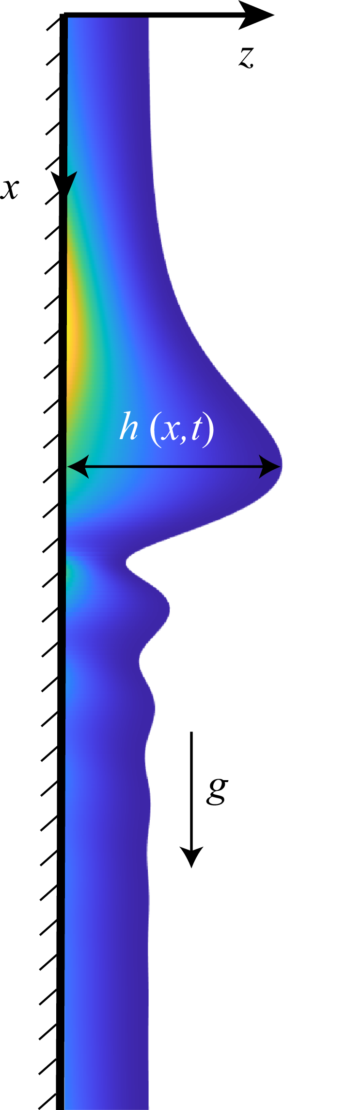

 β=0.5
 Wi=2
 β=0.9
 Wi=10
 (1−β)Wi=1
 Re=1
 Re=10

 ωr,max
 Re
 Wi=2
 β=0.5
 ωr,max
 Wi
 Re=10
 β=0.5

 β=0.5
 Wi=3
 Re=30
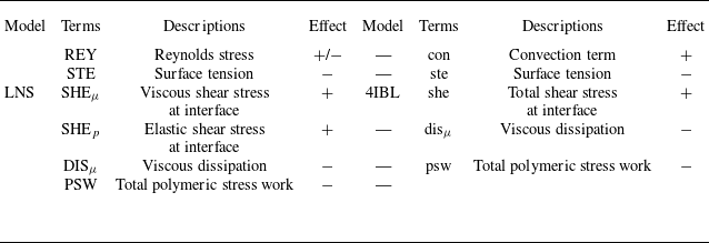
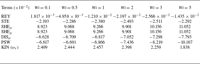
 Wi
 k=0.1
 β=0.5
 Re=30
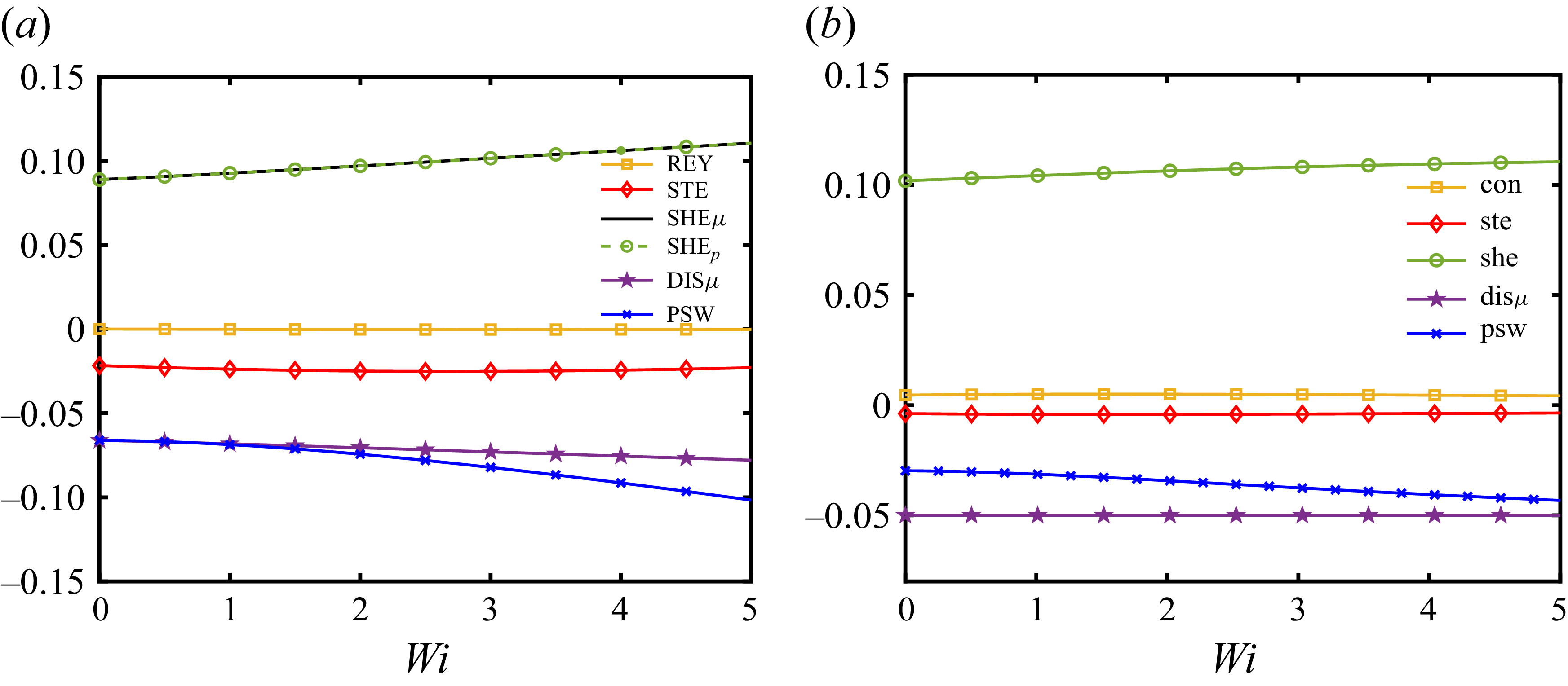
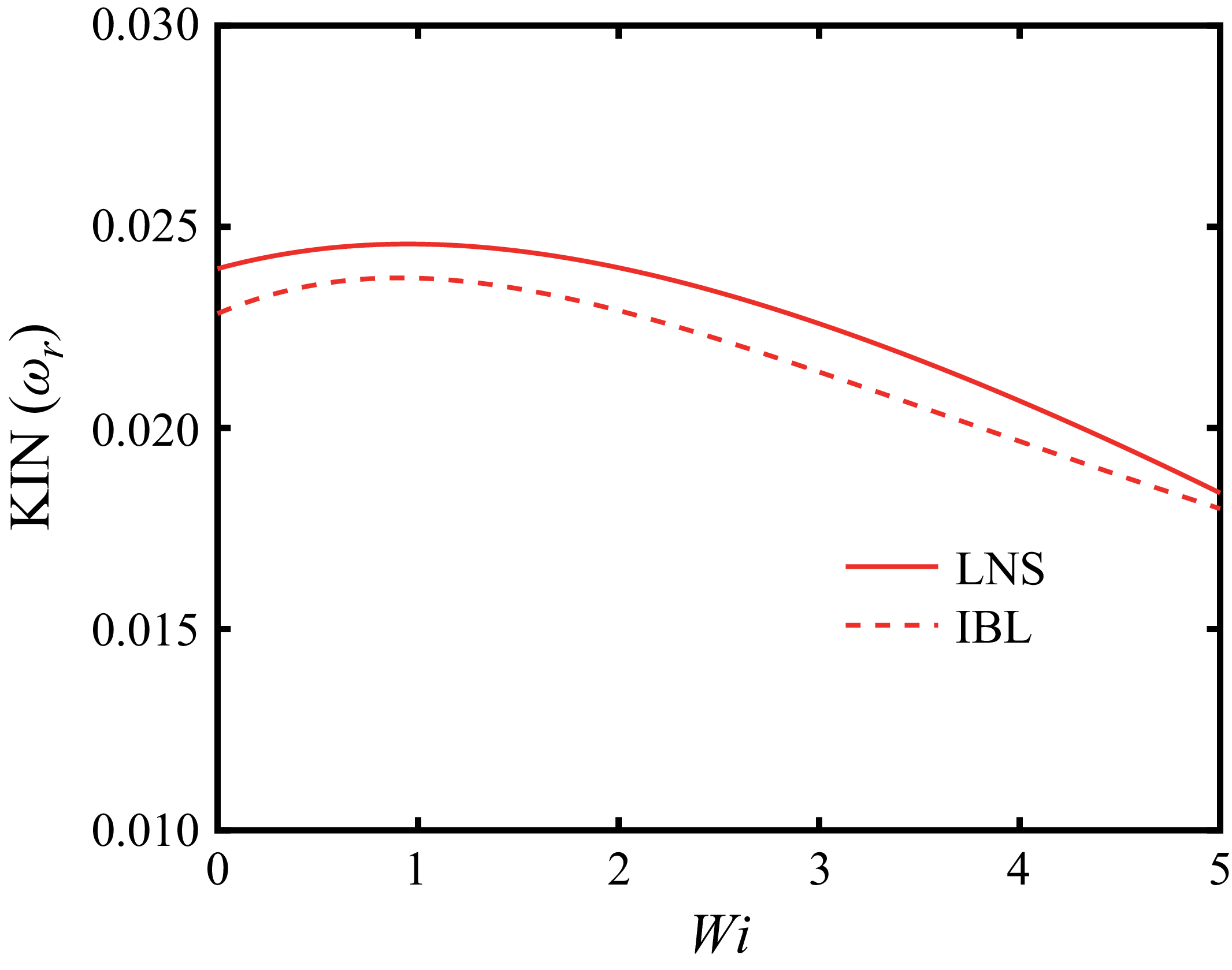
 ωr

 ωr,max
 Re
 Wi
 β=0.5
 β=0.9

 ωr,max
 Wi
 1−β
 k=0.05
 Re=1
 Re=10

 γ2
 γ1
 k=0.01
 Re=10
 β=0.5

 β
 k=0.03
 Re=1
 Re=10
 Re=30
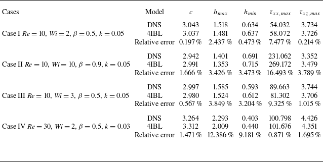
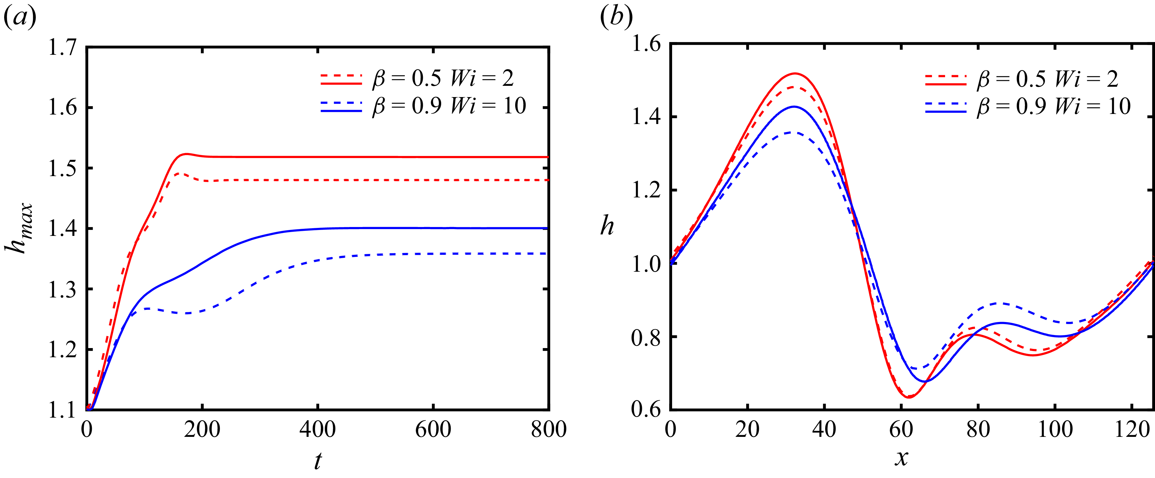
 β=0.5
 Wi=2
 β=0.9
 Wi=10
 hmax
 t

 τxx
 τxz

 τxx
 τxz

 Re=10
 k=0.05
 β=0.5
 hmax
 t

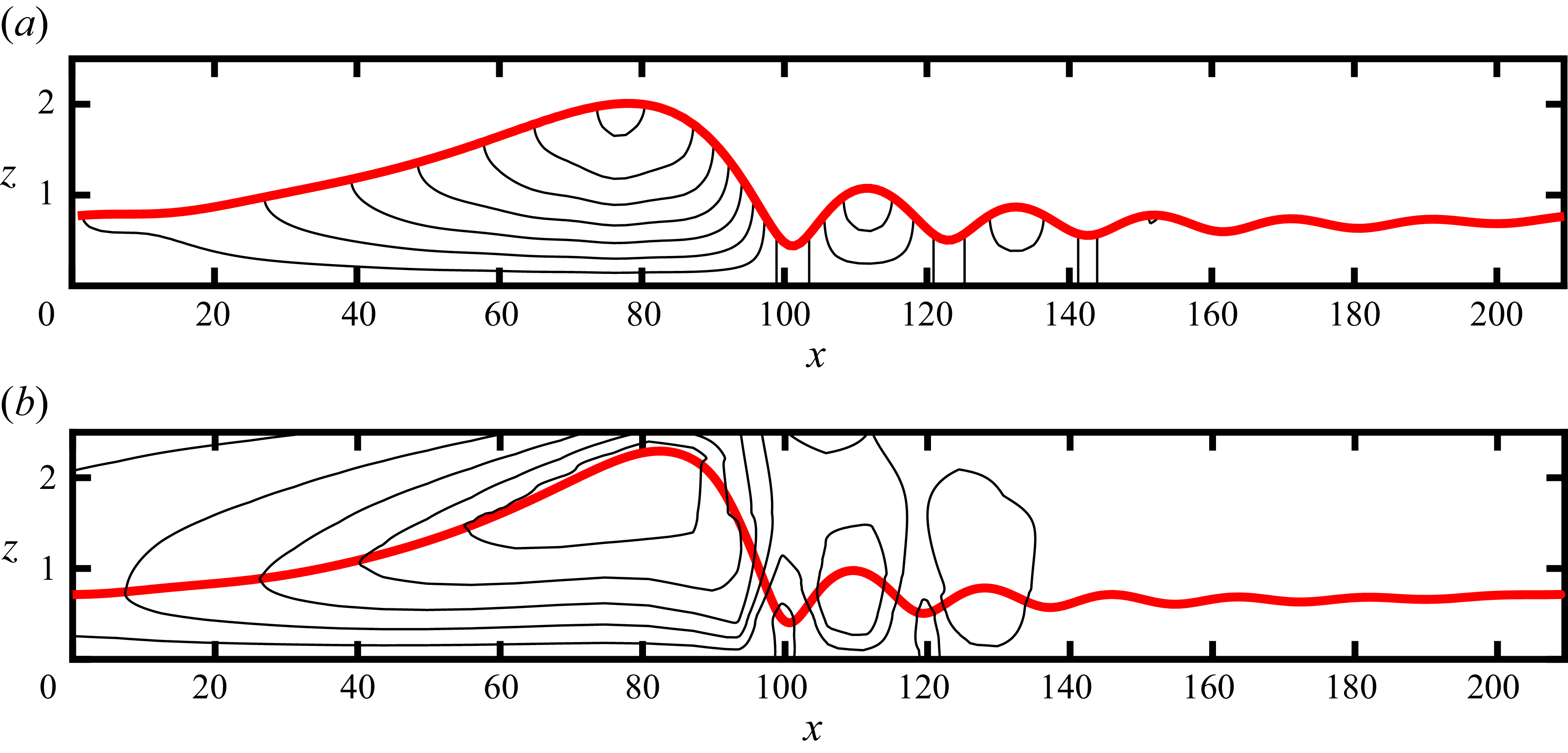
 u=0


