1. Introduction
Magnetoconvection occurs widely in nature, such as thermal convection in the Earth’s outer core and solar convection (see, e.g. Proctor & Weiss Reference Proctor and Weiss1982), as well as in engineering applications, including liquid metal batteries (see, e.g. Kelley & Weier Reference Kelley and Weier2018) and blankets in nuclear fusion reactors (Salavy, Boccaccini & Lässer Reference Salavy, Boccaccini and Lässer2007). The interaction between magnetic fields and convective flows in electrically conducting fluids can profoundly reshape the flow patterns and modify the heat transport of the system. Rayleigh–Bénard convection (RBC) (Ahlers, Grossmann & Lohse Reference Ahlers, Grossmann and Lohse2009; Lohse & Xia Reference Lohse and Xia2010; Chillà & Schumacher Reference Chillà and Schumacher2012; Xia et al. Reference Xia, Huang, Xie and Zhang2023; Lohse & Shishkina Reference Lohse and Shishkina2024) under an externally imposed magnetic field serves as a classical model for studying magnetoconvection, in which a fluid layer is heated from below and cooled from above with a constant temperature difference
 $\Delta T$
. The Rayleigh number
 $Ra = \alpha g \Delta T\! H^3 / (\nu \kappa )$
quantifies the buoyancy forcing, and the Prandtl number
 $\textit{Pr} = \nu / \kappa$
characterises the relative diffusivity of momentum and heat. Here,
 $\alpha$
,
 $\nu$
and
 $\kappa$
are the thermal expansion coefficient, the kinematic viscosity and the thermal diffusivity of the working fluid, respectively. In addition,
 $g$
represents the gravitational acceleration constant, and
 $ H$
is the height of the cell. In confined RBC systems, the aspect ratio
 $\varGamma = D/H$
(where
 $D$
is the lateral dimension) is introduced to characterise the degree of spatial confinement.
For a horizontally infinitely extended fluid layer, also known as bulk magnetoconvection due to the absence of solid sidewalls, Chandrasekhar (Reference Chandrasekhar1952) showed that a vertical magnetic field can significantly suppress the onset of convection with the critical Rayleigh number for the onset of bulk convection
 $Ra_{c,b} \rightarrow \pi ^2 \textit{Ha}^2$
for asymptotically large
 $\textit{Ha}$
. Here,
 $\textit{Ha} = \textit{BH} \sqrt {\sigma /(\rho \nu )}$
is the Hartmann number with
 $B$
,
 $\sigma$
and
 $\rho$
being the magnetic field strength, the electrical conductivity and density of the fluid, respectively. Later experimental studies based on temperature measurements in convection cells with
 $\varGamma \geqslant 1$
attempted to confirm the theoretical prediction of
 $Ra_{c,b}$
(Nakagawa Reference Nakagawa1955; Jirlow Reference Jirlow1956; Cioni, Chaumat & Sommeria Reference Cioni, Chaumat and Sommeria2000), but showed only fair agreement, likely due to the presence of an electrically insulating sidewall and the resulting wall modes. For the characteristic horizontal length scale
 $\ell$
, Chandrasekhar (Reference Chandrasekhar1952) predicted
 $\ell \rightarrow ( \sqrt {2} \pi ) ^{1/3} \textit{Ha}^{-1/3}$
. However, due to the opaqueness of liquid metal, this relation has not yet been tested experimentally, and only very recently has it been verified through two-dimensional direct numerical simulations (DNS) by Bader & Zhu (Reference Bader and Zhu2023).
Unlike bulk convection being treated theoretically, the presence of sidewalls is inevitable in experiments and practical applications. Thus, the stabilising (RBC) or destabilising (rotating RBC and magnetoconvection) effects of the sidewall on convection deserve an in-depth study. Shishkina (Reference Shishkina2021) showed theoretically that the onset of convection can be significantly delayed by spatial confinement with
 $Ra_{c,\varGamma }=(2\pi )^4(1+1.49/\varGamma ^2)(1+0.34/\varGamma ^2)$
for a cylindrical cell. This prediction has been verified in recent studies by Zhang & Xia (Reference Zhang and Xia2023) and Ren et al. (Reference Ren, Tao, Xia and Xie2024). In confined magnetoconvection, the sidewall acts as a destabilisation factor in addition to the stabilising Lorentz force exerted by the applied magnetic field. This destabilisation is due to the decay of the Lorentz force towards the sidewall due to the electrically insulating sidewall boundary condition. It leads to the emergence of a new instability mechanism near the sidewalls, known as wall modes. The onset of magnetic wall modes has been investigated via linear stability analysis (LSA) by Houchens, Witkowski & Walker (Reference Houchens, Witkowski and Walker2002) in cylindrical geometries with only two
 $\varGamma$
, namely 1 and 2, as well as in semi-infinite domains by Busse (Reference Busse2008), where the effect of curvature induced by the sidewall is ignored. These studies revealed that the critical Rayleigh number for the onset of wall modes follows
 $Ra_{c,w} \rightarrow \textit{Ha}^{3/2}$
for asymptotically large
 $\textit{Ha}$
. However, a systematic study on the effects of
 $\varGamma$
and
 $\textit{Ha}$
on the onset of magnetoconvection is missing.
Due to the difficulty in measuring the flow field of opaque liquid metal convection, the study of the wall-mode dynamics after onset is mainly based on DNS with
 $\textit{Pr}\sim 10^{-2}$
in rectangular cells for a limited number of
 $\varGamma$
, i.e.
 $1\leqslant \varGamma \leqslant 4$
. For example, the wall modes are found to exhibit a typical two-layered structure, i.e. a main flow in the upward (downward) direction with a nose-like flow in the downward (upward) direction (Liu, Krasnov & Schumacher Reference Liu, Krasnov and Schumacher2018). Its evolution to chaos with increasing
 $Ra$
is studied in detail by McCormack et al. (Reference McCormack, Teimurazov, Shishkina and Linkmann2023). In addition, the wall modes are found to enhance heat transport of the system (Wu, Chen & Ni Reference Wu, Chen and Ni2025).
On the experimental side, the wall-mode dynamics is mainly studied based on temperature signals measured close to the sidewall in cylindrical cells with
 $\varGamma =1$
and 2. Zürner et al. (Reference Zürner, Schindler, Vogt, Eckert and Schumacher2020) show how the magnetic field suppresses the large-scale circulation in turbulent RBC and transforms the flow to cellular structures that may correspond to wall modes. Xu, Horn & Aurnou (Reference Xu, Horn and Aurnou2023) show that the steady wall modes could transition to structures with different azimuthal mode numbers with increasing
 $Ra$
. In a DNS study similar to Xu et al. (Reference Xu, Horn and Aurnou2023), the wall modes are found to drift azimuthally (Akhmedagaev et al. Reference Akhmedagaev, Zikanov, Krasnov and Schumacher2020). This drift is speculated to result from collisions between wall-mode ejections, as suggested by Xu et al. (Reference Xu, Horn and Aurnou2023).
The studies mentioned above have enriched our understanding of wall-mode formation and its evolution with respect to
 $Ra$
. However, one question remains: Do wall modes appear as long as the convection domain is confined with insulating sidewalls? To answer this, one needs to study the wall-mode dynamics over a much wider range of
 $\varGamma$
beyond that reported in the literature, which serves as the motivation of the present study.
It should be noted that wall modes are also observed in rotating RBC (see, e.g. Zhong, Ecke & Steinberg Reference Zhong, Ecke and Steinberg1991). They also exhibit a two-layer structure, similar to magnetoconvection (Zhang et al. Reference Zhang, Reiter, Shishkina and Ecke2024). However, unlike the steady nature of magnetic wall modes, depending on the boundary conditions, prograde or retrograde wall modes are observed in rotating convection (Ravichandran & Wettlaufer Reference Ravichandran and Wettlaufer2024; Vasil et al. Reference Vasil, Burns, Lecoanet, Oishi, Brown and Julien2025). The different dynamics of the wall modes may stem from the fact that rotation introduces a preferred direction, whereas the magnetic field does not break the horizontal symmetry of the system. Thus, the study of wall modes in magnetoconvection may also advance our understanding of wall modes in rotating RBC.
In this paper, using LSA, we will show that the onset of wall modes in confined magnetoconvection is a result of the interplay between spatial confinement and the magnetic field. No wall mode can be observed in the strongly confined regime. We will give the conditions for the emergence of wall modes and their evolution with
 $\varGamma$
and
 $\textit{Ha}$
. We will also outline a phase diagram in the
 $\varGamma$
–
 $\textit{Ha}$
space to delineate the dominating factors that determine the onset of wall modes and bulk convection. These findings provide practical guidelines for experimental and numerical studies on the wall-mode dynamics in liquid metal magnetoconvection.
2. The model system and the LSA method
2.1. The model system
We consider magnetoconvection in a cylindrical cell subjected to a uniform external vertical magnetic field. The classical RBC always sets in as stationary convection, both in an infinite layer and in wall-bounded systems (Chandrasekhar Reference Chandrasekhar1961; Ren et al. Reference Ren, Tao, Xia and Xie2024). When a magnetic field is introduced, the instability remains stationary if the thermal diffusivity
 $\kappa$
of the fluid is smaller than its magnetic diffusivity
 $\eta$
; whereas, when
 $\kappa$
exceeds
 $\eta$
, complex eigenvalues arise and oscillatory instabilities appear, as demonstrated by Chandrasekhar (Reference Chandrasekhar1952). The presence of sidewalls is not expected to alter the temporal dynamics of the onset of convection. As most laboratory studies of magnetoconvection use liquid metals with
 $\kappa \ll \eta$
(see, e.g. Zürner et al. Reference Zürner, Schindler, Vogt, Eckert and Schumacher2020; Ren et al. Reference Ren, Tao, Zhang, Ni, Xia and Xie2022), the onset of wall modes therefore sets in as stationary convection. Note that the stationary onset has also been confirmed by experiments and DNS in magnetoconvection in cylindrical cells (Xu et al. Reference Xu, Horn and Aurnou2023). Accordingly, similar to the studies by Busse (Reference Busse2008) and Bhattacharya et al. (Reference Bhattacharya, Boeck, Krasnov and Schumacher2024), we treat the onset of convection as a stationary process and ignore the time-dependent terms in the governing equations.
Under the Oberbeck–Boussinesq approximation (Oberbeck Reference Oberbeck1879; Boussinesq Reference Boussinesq1903) and quasi-static approximation (Moreau Reference Moreau1990), the linearised time-independent governing equations of magnetoconvection are as follows:
 \begin{equation} -\boldsymbol{\nabla \!} p+\boldsymbol{\nabla }^2\boldsymbol{u}+\textit{Ha}^2(\boldsymbol{J}\times \hat {\boldsymbol{e}}_{\boldsymbol{z}})+RaT\hat {\boldsymbol{e}}_{\boldsymbol{z}}=0, \\[-12pt] \nonumber \end{equation}
 \begin{equation} {\boldsymbol{\nabla }}^2 T + \hat {\boldsymbol{e}}_{\boldsymbol{z}}\boldsymbol{\cdot } \boldsymbol{u}=0, \\[-12pt] \nonumber \end{equation}
 \begin{equation} \boldsymbol{J}=-\boldsymbol{\nabla }\phi +(\boldsymbol{u} \times \hat {\boldsymbol{e}}_{\boldsymbol{z}}), \\[-12pt] \nonumber \end{equation}
 \begin{equation} \boldsymbol{\nabla }\boldsymbol{\cdot }\boldsymbol{u} = 0, \\[-12pt] \nonumber \end{equation}
 \begin{equation} \boldsymbol{\nabla }\boldsymbol{\cdot }\boldsymbol{J} = 0, \end{equation}
where
 $\boldsymbol{u}$
,
 $\boldsymbol{J}$
,
 $p$
,
 $\phi$
and
 $T$
represent fluctuation fields of the velocity, electrical current density, generalised pressure, electric potential and temperature. The symbol
 $\hat {\boldsymbol{e}}_{\boldsymbol{z}}$
is the unit vector in the vertical direction. The base state considered here is the conduction state with zero velocity and a linear vertical temperature distribution. Equations (2.1)–(2.5) have been non-dimensionalised using
 $H$
,
 $\Delta T$
,
 $B$
, the diffusion time scale
 $H^2/\kappa$
and the velocity scale
 $\kappa /H$
. From the governing equations, it can be seen that the linearised system is governed by two dimensionless control parameters: the Hartmann number
 $\textit{Ha}$
, measuring the strength of the magnetic field, and the Rayleigh number
 $Ra$
, quantifying the buoyancy force. As the Prandtl number
 $\textit{Pr}$
does not explicitly appear in the above equations, the critical Rayleigh number
 $Ra_c$
for the onset of convection is independent of
 $\textit{Pr}$
. Note that this property does not depend on the particular choice of non-dimensionalisation. For instance, if one adopts the non-dimensionalisation commonly used in DNS, where the free-fall velocity and free-fall time are taken as the characteristic velocity and time scales, one arrives at the same set of governing equations.
2.2. The linear stability analysis method
To account for the effect of spatial confinement, i.e. varying the aspect ratio
 $\varGamma$
, the diameter
 $D$
is used to renormalise the horizontal coordinate
 $r$
during LSA. This procedure will introduce
 $\varGamma$
into the differential operators, and keep the governing (2.1)–(2.5) unchanged. For example, the Laplacian
 $\boldsymbol{\nabla }^2$
is modified to be
 \begin{equation} {\nabla }^2=\frac {4}{\varGamma ^2}\frac {1}{r}\frac {\partial }{\partial r}r\frac {\partial }{\partial r} + \frac {4}{\varGamma ^2r^2}\frac {\partial ^2 }{\partial \theta ^2} +\frac {\partial ^2 }{\partial z^2}. \end{equation}
The no-penetration and no-slip conditions are applied for the velocity field on all the boundaries. The isothermal conditions are applied on the top and bottom boundaries, and adiabatic temperature boundary conditions are applied at the sidewall. The insulating electrical boundary conditions are imposed on all walls. These boundary conditions can be written as follows:
 \begin{equation} u_r=u_{\phi }=u_z=T=\frac {\partial \phi }{\partial z}=0 \,\,(z=\pm 1/2),\\[-12pt] \nonumber \end{equation}
 \begin{equation} u_r=u_{\phi }=u_z=\frac {\partial T}{\partial r}=\frac {\partial \phi }{\partial r}=0 \,\,(r=1). \end{equation}
In convection systems, as
 $Ra$
increases, the vertical single-roll structure is always the first mode to become unstable. With further increase in
 $Ra$
, the vertically stacked multiple-roll structure will become unstable, as demonstrated by Ren et al. (Reference Ren, Tao, Xia and Xie2024). Therefore, we restrict our attention to the instability of the vertical single-roll modes. In this case, the temperature field of the flow can be approximated as
 \begin{equation} T\cong \sum _{j = 1}^{K} \sum _{m = 1}^{M}H_{\textit{jm}}T_{\textit{jm}};\,\,\,T_{\textit{jm}}=\cos {(n\theta )}\cos {((2m-1)\pi z)}J_n(\beta _{nj}r), \end{equation}
where
 $H_{\textit{jm}}$
are the coefficients corresponding to the basis functions
 $T_{\textit{jm}}$
. The
 $j$
and
 $m$
are the indices of the radial (
 $r-$
) and vertical (
 $z-$
) modes, respectively;
 $K$
and
 $M$
are the corresponding truncation numbers; and
 $n$
is the azimuthal (
 $\theta \hbox{-}$
) mode number (e.g.
 $n=0$
for the axisymmetric mode and
 $n\gt 0$
for asymmetric modes). Also,
 $J_n$
is the
 $n$
th-order regular Bessel function of the first kind, and
 $\beta _{nj}$
are the zeros of
 ${\rm d}J_n/{\rm d}r$
.
Note that, for ease of analysis, the velocity field for the azimuthally axisymmetric mode with
 $n=0$
and the asymmetric modes with
 $n\gt 0$
are considered separately. For the axisymmetric mode, a streamfunction
 $\psi$
can be defined to express a series of solenoid fields that can be used to approximate the velocity field
 \begin{equation} \boldsymbol{u}\cong \sum _{j = 1}^{K} \sum _{m = 1}^{M}A_{\textit{jm}}\boldsymbol{U}_{\textit{jm}};\,\,\, \boldsymbol{U}_{\textit{jm}}=\boldsymbol{\nabla } \times (\psi _{\textit{jm}}\hat {\boldsymbol{e}}_{\boldsymbol{\theta }}), \end{equation}
where
 $A_{\textit{jm}}$
are the coefficients corresponding to the basis functions
 $\boldsymbol{U}_{\textit{jm}}$
. To satisfy the boundary conditions, the streamfunction
 $\psi$
is constructed as follows:
 \begin{equation} \psi _{\textit{jm}}=C_m(z)\left (\frac {J_1(\alpha _jr)}{J_1(\alpha _j)}-\frac {I_1(\alpha _jr)}{I_1(\alpha _j)}\right )\!;\, C_m(z)=\left ( \frac {\cosh {\lambda _m z}}{\cosh {\frac {1}{2}\lambda _m}}-\frac {\cos {\lambda _m z}}{\cos {\frac {1}{2}\lambda _m}} \right ) \!. \end{equation}
Here,
 $C_m(z)$
is the even beam function (Reid & Harris Reference Reid and Harris1958) and
 $\lambda _m$
are the roots of
 \begin{equation} \tanh {\frac {1}{2}\lambda _m}+\tan {\frac {1}{2}\lambda _m}=0, \end{equation}
where
 $I_n$
is the
 $n$
th-order modified Bessel function of the first kind, and
 $\alpha _j$
are the roots of
 \begin{equation} I_1(\alpha _j)J_2(\alpha _j)+J_1(\alpha _j)I_2(\alpha _j)=0. \end{equation}
As for the electric potential field
 $\phi$
, no basis function is required, since the Poisson source term for
 $\phi$
vanishes due to axisymmetry. This can be straightforwardly shown by substituting (2.10) into (2.3) and (2.5).
For the asymmetric modes (
 $n\gt 0$
), following Buell & Catton (Reference Buell and Catton1983), the velocity field can be constructed from two two-dimensional velocity fields
 \begin{equation} \boldsymbol{u}=\boldsymbol{U}^{(1)}+\boldsymbol{U}^{(2)} , \end{equation}
where
 \begin{equation} \boldsymbol{U}^{(1)}\cong \sum _{j = 1}^{K} \sum _{m = 1}^{M}B_{\textit{jm}}\boldsymbol{U}_{\textit{jm}}^{(1)};\, \boldsymbol{U}_{\textit{jm}}^{(1)}=\boldsymbol{\nabla } \times (\varphi _{\textit{jm}}\hat {\boldsymbol{e}}_{\boldsymbol{r}}) , \\[-9pt] \nonumber \end{equation}
 \begin{equation} \boldsymbol{U}^{(2)}\cong \sum _{j = 1}^{K} \sum _{m = 1}^{M}D_{\textit{jm}}\boldsymbol{U}_{\textit{jm}}^{(2)};\, \boldsymbol{U}_{\textit{jm}}^{(2)}=\boldsymbol{\nabla } \times (\zeta _{\textit{jm}}\hat {\boldsymbol{e}}_{\boldsymbol{z}}). \end{equation}
Here,
 $B_{\textit{jm}}$
and
 $D_{\textit{jm}}$
are the coefficients corresponding to the basis functions
 $\boldsymbol{U}_{\textit{jm}}^{(1)}$
and
 $\boldsymbol{U}_{\textit{jm}}^{(2)}$
, respectively. To satisfy the boundary conditions, the basis functions are constructed as follows:
 \begin{equation} \varphi _{\textit{jm}}=\sin {(n\theta )}C_m(z)J_{n+1}(\delta _{nj}r);\quad \zeta _{\textit{jm}}=\sin {(n\theta )}\sin {(2\pi mz)}\left (\frac {J_n(\omega _{nj}r)}{J_n(\omega _{nj})}-\frac {I_n(\omega _{nj}r)}{I_n(\omega _{nj})}\right )\! , \end{equation}
where
 $\delta _{nj}$
and
 $\omega _{nj}$
are the roots of
 \begin{equation} J_{n+1}(\delta _{nj})=0;\quad J_n(\omega _{nj})I_{n+1}(\omega _{nj})+I_n(\omega _{nj})J_{n+1}(\omega _{nj})=0. \end{equation}
The electric potential field
 $\phi$
can be constructed as follows:
 \begin{equation} \phi \cong \sum _{j = 1}^{K} \sum _{m = 1}^{M}G_{\textit{jm}}\phi _{\textit{jm}};\quad \phi _{\textit{jm}}=\sin {(n\theta )}\sin {((2m-1)\pi z)}J_n(\gamma _{nj}r), \end{equation}
where
 $G_{\textit{jm}}$
are the coefficients corresponding to the basis functions
 $\phi _{\textit{jm}}$
, and
 $\gamma _{nj}$
are the zeros of
 ${\rm d}J_n/{\rm d}r$
.
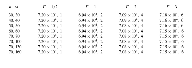
Critical Rayleigh number (
 $Ra_c$
) and azimuthal mode number (
 $n$
) obtained for different values of
 $K$
and
 $M$
, with
 $\textit{Ha} = 100$
. Note in each data entry, the first value denotes
 $Ra_c$
and the second value denotes
 $n$
.

Then the Galerkin method is applied to reduce the analysis to an eigenvalue problem (Buell & Catton Reference Buell and Catton1983), from which the critical Rayleigh number
 $Ra_c$
and the corresponding flow pattern are obtained. Further details of the LSA are given in Appendix A.
2.3. The accuracy and validation of the LSA results
To assess the accuracy of LSA, we carried out a convergence test by varying the number of truncation functions
 $K$
and
 $M$
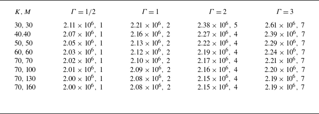
. Tables 1 and 2 list the critical Rayleigh number
 $Ra_c$
and the azimuthal mode number
 $n$
for different
 $\varGamma$
with
 $\textit{Ha}=100$
and
 $\textit{Ha}=1000$
, respectively. In general, a higher number of truncation functions is required for larger
 $\varGamma$
and higher
 $\textit{Ha}$
. For
 $\textit{Ha}=100$
,
 $K=M=30$
is sufficient to ensure convergence of the azimuthal mode number
 $n$
, and the critical Rayleigh number
 $Ra_c$
is obtained with an accuracy better than
 $0.5\,\%$
. For the largest Hartmann number explored in this study, i.e.
 $\textit{Ha} = 1000$
, full convergence of the azimuthal mode number
 $n$
is already achieved at
 $K=M=40$
. However, for the critical Rayleigh number
 $Ra_c$
, data with
 $K$
and
 $M$
increasing from 30 to 70 exhibit a monotonic convergence. Taking the relative change of
 $Ra_c$
between
 $K=M=60$
and
 $K=M=70$
, as an estimate of the accuracy of the LSA, the relative variations are approximately
 $0.50\,\%$
for
 $\varGamma =1/2$
,
 $0.95\,\%$
for
 $\varGamma =1$
,
 $0.92\,\%$
for
 $\varGamma =2$
and
 $1.36\,\%$
for
 $\varGamma =3$
. To further examine the influence of properly resolving the Hartmann boundary layers, which appear under a strong magnetic field, on the convergence of
 $Ra_c$
, we increased the vertical resolution up to
 $M = 160$
. It can be seen from table 2 that, for the largest Hartmann number considered (i.e.
 $\textit{Ha} = 1000$
), the case with
 $K = M = 70$
already achieves an accuracy within
 $1\,\%$
. The results indicate that the
 $Ra_c$
obtained from the present LSA may not be sensitive to fully resolving the Hartmann boundary layers. Since the present work mainly focuses on
 $Ra_c$
and the horizontal length scales, we use
 $K = 70$
and
 $M = 160$
for
 $\textit{Ha} = 1000$
, while for the other cases we adopt
 $K = M = 70$
to reduce the computational cost. By doing so, the azimuthal structures of the wall modes are well resolved, and the resulting accuracy of
 $Ra_c$
is better than
 $1\,\%$
.
Critical Rayleigh number (
 $Ra_c$
) and azimuthal mode number (
 $n$
) obtained for different values of
 $K$
and
 $M$
, with
 $\textit{Ha} = 1000$
. Note in each data entry, the first value denotes
 $Ra_c$
and the second value denotes
 $n$
.

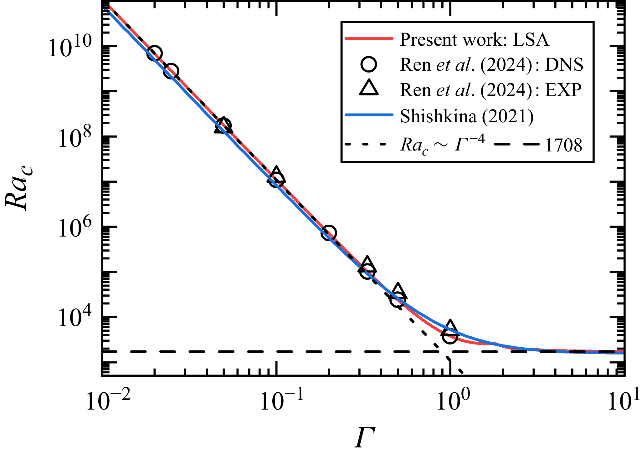
To validate the present LSA results, we compare them with the results reported in the literature. Figure 1 shows the
 $Ra_c$
curve obtained in the present work as a function of
 $\varGamma$
for
 $\textit{Ha}=0$
. The curve (see also figures 2, 3
a,d, 4
a) consists of several hundred logarithmically evenly spaced points for smoothness. For
 $\varGamma \leqslant 1/10$
, the present data can be fitted by
 $Ra_c = 1090\varGamma ^{-4.0}$
, as indicated by the dotted line. Whereas for large
 $\varGamma$
, the values of
 $Ra_c$
approach
 $1708$
, corresponding to the critical Rayleigh number for the onset of convection in the infinite-layer limit with no-slip boundaries. For comparison, we plot the
 $Ra_c$
values from Ren et al. (Reference Ren, Tao, Xia and Xie2024), which were measured experimentally and also obtained numerically in liquid gallium-indium-tin alloy convection without a magnetic field. One observes that the present LSA results are in good agreement with the DNS and experimental results. The theoretical prediction
 $Ra_{c,\varGamma } = (2\pi )^4(1+1.49/\varGamma ^2)(1+0.34/\varGamma ^2)$
from Shishkina (Reference Shishkina2021) is also shown here, which yields similar results, although the approach by Shishkina (Reference Shishkina2021) is essentially different from LSA. For
 $\textit{Ha}\gt 0$
, the present LSA results are in good agreement with previous stability analyses (see the discussion of figure 2 in § 3). However, to the best of our knowledge, no experimental or DNS data on the onset of wall modes are available for direct comparison, as none have directly and accurately determined the critical Rayleigh number
 $Ra_c$
for the onset of wall modes. Fortunately, a DNS study very close to the wall-mode onset was reported in Xu et al. (Reference Xu, Horn and Aurnou2023) with
 $\textit{Ha}=200$
,
 $\varGamma =2$
, and
 $Ra=2.0\times 10^5$
. The wall-mode structure was characterised by an azimuthal mode number
 $n=4$
, and the case yielded
 $Nu=1.004$
, indicating that it is very close to onset. For the same parameters, our present LSA yields
 $Ra_c=1.94\times 10^5$
with
 $n=4$
, showing excellent agreement with the data from Xu et al. (Reference Xu, Horn and Aurnou2023). The agreement between the present LSA results and those published in the literature provides confidence in the results presented below.
3. Results and discussions
3.1. The critical Rayleigh number
 $Ra_c$
for the onset of convection

In this subsection, we discuss the effects of spatial confinement and magnetic field on the critical Rayleigh number
 $Ra_c$
for the onset of convection. As previous studies typically examined the effect of the magnetic field on
 $Ra_c$
under a fixed geometrical configuration, we follow this perspective and investigate the dependence of
 $Ra_c$
on
 $\textit{Ha}$
for a given
 $\varGamma$
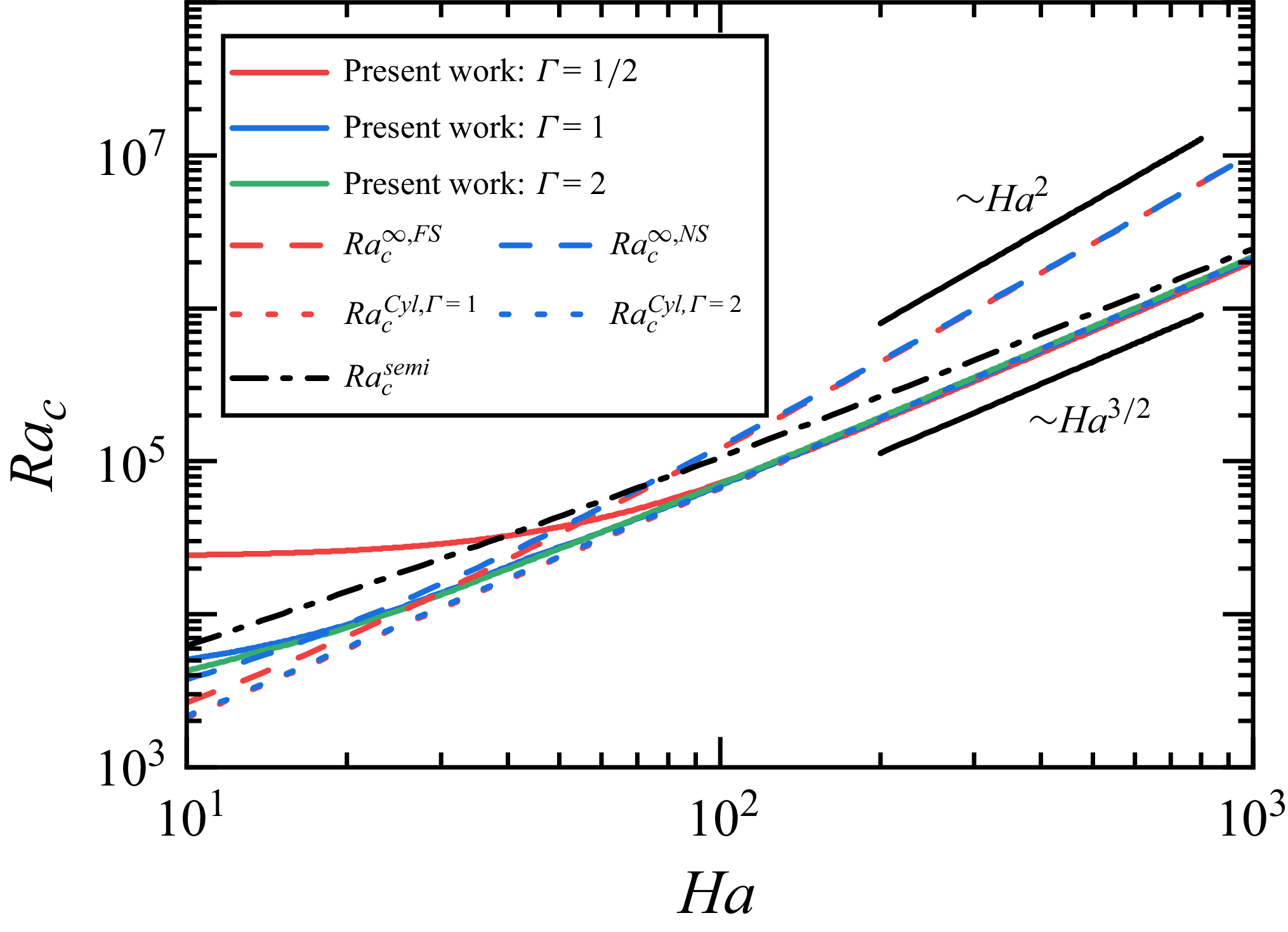
. In an infinite fluid layer, only bulk convection sets in. The critical Rayleigh numbers
 $Ra_c^{\infty {,FS}}$
and
 $Ra_c^{\infty {,NS}}$
, corresponding to free-slip and no-slip top and bottom boundaries, respectively, were derived by Chandrasekhar (Reference Chandrasekhar1952) and both scale as
 $\textit{Ha}^2$
in the limit of large
 $\textit{Ha}$
, as shown in figure 2. Note that
 $Ra_c^{\infty {,NS}}$
is denoted as
 $Ra_{c,b}$
elsewhere in the present paper to reflect its physical meaning. With the presence of sidewalls, wall-mode onset can occur. Figure 2 also presents the
 $Ra_c$
vs
 $\textit{Ha}$
curves for
 $\varGamma =1/2$
,
 $1$
and
 $2$
obtained from the present work. It can be observed that the three curves with different
 $\varGamma$
converge and approach the
 $\textit{Ha}^{3/2}$
scaling when
 $\textit{Ha}\gt 100$
. In addition, a
 $\varGamma$
-dependence of
 $Ra_c$
appears when
 $\textit{Ha}\lt 100$
, namely
 $Ra_c$
for
 $\varGamma =1/2$
is higher than that of
 $\varGamma =1$
and
 $2$
, suggesting spatial confinement also affects the onset of magnetoconvection.
The critical Rayleigh number
 $Ra_c$
vs
 $\varGamma$
at
 $\textit{Ha}=0$
. The dotted line marks
 $Ra_c \sim \varGamma ^{-4}$
fitted to the data with
 $\varGamma \leqslant 1/10$
. The horizontal dashed line presents
 $Ra_c=1708$
for
 $\textit{Ha}=0$
in an infinite layer with no-slip boundaries. Circles and triangles denote DNS and experimental data from Ren et al. (Reference Ren, Tao, Xia and Xie2024), respectively. The blue solid line shows the theoretical prediction from Shishkina (Reference Shishkina2021).

The critical Rayleigh number
 $Ra_c$
vs
 $\textit{Ha}$
for different
 $\varGamma$
. The solid lines are results from the present work. The red and blue dashed lines represent the results for an infinite layer with free-slip and no-slip boundaries, respectively, from Chandrasekhar (Reference Chandrasekhar1952). The red and blue dotted lines indicate the asymptotic solutions for cylinders with
 $\varGamma =1$
and
 $\varGamma =2$
, respectively, from Houchens et al. (Reference Houchens, Witkowski and Walker2002). The black dash-dotted line corresponds to an asymptotic solution along a straight vertical sidewall in a semi-infinite domain with free-slip top and bottom boundaries from Busse (Reference Busse2008).

(a,d) The critical Rayleigh number
 $Ra_c$
vs
 $\varGamma$
at
 $\textit{Ha}=100$
and
 $\textit{Ha}=1000$
, respectively, for different azimuthal modes
 $n$
. The minimum
 $Ra_{c,n}$
for each
 $\varGamma$
forms the
 $Ra_c$
curve highlighted with a solid line. The black horizontal dashed line indicates
 $Ra_{c,b}$
for the onset of bulk convection for comparison. (b,c) Flow structures for
 $\varGamma =2$
and
 $\varGamma =3$
at
 $\textit{Ha}=100$
. (e, f) Flow structures for
 $\varGamma =2$
and
 $\varGamma =3$
at
 $\textit{Ha}=1000$
. The colour represents the contours of the normalised vertical velocity
 $U_z / \max {|U_z|}$
.

(a) The
 $Ra_c$
vs
 $\varGamma$
curves for different
 $\textit{Ha}$
. The horizontal dashed lines mark
 $Ra_{c,b}$
for the onset of bulk convection. (b) Phase diagram showing the dominating factors that determine
 $Ra_c$
. In regime I,
 $Ra_c = 1090\varGamma ^{-4.0}$
and is determined by
 $\varGamma$
. In regimes II and III the co-action of geometrical confinement and magnetic field determines
 $Ra_c$
with no wall modes in regime II and wall modes developing in regime III. Regime IV is the wall-mode-dominated regime with
 $Ra_c=Ra_{c,w} \approx 65 \textit{Ha}^{1.5}$
, determined by the magnetic field. Refer to the main text for the meanings of the remaining symbols.

For comparison, the
 $Ra_c$
vs
 $\textit{Ha}$
curves from previous LSA are also shown. For large
 $\textit{Ha}$
in cylindrical cells with
 $\varGamma =1$
and
 $2$
, Houchens et al. (Reference Houchens, Witkowski and Walker2002) show
 $Ra_c^{\textit{Cyl},\,\varGamma =1}=66.417\textit{Ha}^{3/2}$
and
 $Ra_c^{\textit{Cyl},\,\varGamma =2}=67.748\textit{Ha}^{3/2}$
, respectively. It can be observed that the
 $Ra_c$
vs
 $\textit{Ha}$
curves by Houchens et al. (Reference Houchens, Witkowski and Walker2002) are in excellent agreement with the present results for
 $\textit{Ha}\gt 100$
, further validating the present work. However, for
 $\textit{Ha}\lt 100$
, one observes some discrepancy between the two studies, which may be because the asymptotic solution calculated by Houchens et al. (Reference Houchens, Witkowski and Walker2002) requires large
 $\textit{Ha}$
to be accurate. The
 $Ra_c$
vs
 $\textit{Ha}$
curve for a straight vertical sidewall in a semi-infinite domain with free-slip top and bottom boundaries calculated by Busse (Reference Busse2008) is also plotted as a dash-dotted line for comparison. One sees that, although the data for configurations with sidewalls all show
 $Ra_c\sim \textit{Ha}^{3/2}$
scaling for large enough
 $\textit{Ha}$
, the magnitudes of the curves for a semi-infinite domain and those for the finite aspect ratio domains differ within the range of
 $10\lt Ha \lt 10^3$
. This deviation may be due to the use of free-slip boundary conditions and the neglect of curvature effects in the analysis by Busse (Reference Busse2008).
Figure 2 also shows that the difference between the
 $\textit{Ha}^2$
curve for the bulk convection onset and the
 $\textit{Ha}^{3/2}$
curves for the wall-mode onset becomes larger with increasing
 $\textit{Ha}$
. Due to the observation that wall modes are located in the vicinity of the sidewalls, these modes are not expected to significantly affect the onset of convection in the bulk when
 $\varGamma$
is very large or
 $\textit{Ha}$
is very large. Specifically, in such a system, as
 $Ra$
increases, wall modes first occur when
 $Ra \gt Ra_{c,w}$
, while the bulk convection onset appears when
 $Ra \gt Ra_{c,b}$
. This observation indicates that a larger
 $\textit{Ha}$
yields a wider
 $Ra$
interval in which pure wall modes exist, which provides a platform to study the evolution of wall modes with minimal influence from the bulk convection.
Having discussed the effect of
 $\textit{Ha}$
on
 $Ra_c$
for a given
 $\varGamma$
, we now turn to a systematic investigation of the dependence of
 $Ra_c$
on
 $\varGamma$
at fixed
 $\textit{Ha}$
. Let us first focus on the case with
 $\textit{Ha}=100$
. For a given azimuthal mode number
 $n$
, we can obtain
 $Ra_{c,n}$
as a function of
 $\varGamma$
. The results are shown in figure 3(a). The horizontal dashed line in this figure marks the critical Rayleigh number for the bulk onset
 $Ra_{c,b}$
, corresponding to a horizontally periodic system with no-slip boundaries at the top and bottom, as reported by Chandrasekhar (Reference Chandrasekhar1952). For the case with
 $n=0$
, one observes that
 $Ra_{c,n=0}$
approaches
 $Ra_{c,b}$
with increasing
 $\varGamma$
, but it does not drop below
 $Ra_{c,b}$
, suggesting that the axisymmetric wall modes do not occur at the onset of convection. For
 $n \geqslant 1$
, one sees the
 $Ra_{c,n}$
curves all drop below
 $Ra_{c,b}$
, suggesting that wall modes emerge. To determine the
 $Ra_c(\varGamma )$
value, we locate the minimum value among all
 $Ra_{c,n}$
for each
 $\varGamma$
. The so-obtained
 $Ra_c(\varGamma )$
curves are highlighted with solid lines. It is seen that, with increasing
 $\varGamma$
, the most unstable azimuthal mode changes, resulting in unsmooth changes in the
 $Ra_c(\varGamma )$
curve. In addition, for a given
 $n$
,
 $Ra_c(\varGamma )$
first decreases and then increases with
 $\varGamma$
, and the range of
 $\varGamma$
when the system is in a particular mode number
 $n$
decreases with increasing
 $n$
. Note that the
 $n=8$
curve is shown as a whole dotted line, since higher modes with
 $n\gt 8$
were not computed due to the limitation of computational resources. We thus have no information on the
 $Ra_c(\varGamma )$
curve for
 $n \geqslant 8$
.
To gain better insight into the structure of the wall modes, we show the vertical velocity contours of the flow for
 $\varGamma = 2$
and
 $3$
in figures 3(b) and 3(c), respectively. The colour represents the normalised vertical velocity
 $U_z / \max {|U_z|}$
. One sees that their respective mode numbers are
 $n=4$
and 6. The wall modes are confined near the sidewall region, and they exhibit typical two-layer structures with opposite velocity directions, i.e. a main flow in the upward (downward) direction with a nose-like flow in the downward (upward) direction. The vertical velocity in the bulk region remains essentially zero. The two-layer structure is similar to DNS studies beyond the onset of wall modes reported in the literature (Liu et al. Reference Liu, Krasnov and Schumacher2018; Xu et al. Reference Xu, Horn and Aurnou2023; McCormack et al. Reference McCormack, Teimurazov, Shishkina and Linkmann2023). However, due to there being no information on
 $Ra_{c,w}$
in realistic confined geometries,
 $Ra_{c,b}$
is usually employed as a measure in these studies. Figure 3(d)–( f) shows the same quantities as figure 3(a)–(c), but for
 $\textit{Ha}=1000$
, where higher
 $Ra_c$
values and thinner wall-mode structures are observed. We also note that the azimuthal mode number changes to
 $n=4$
for
 $\varGamma =2$
and
 $n=7$
for
 $\varGamma =3$
.
To study the effects of
 $\textit{Ha}$
and
 $\varGamma$
on the onset of magnetoconvection, we show in figure 4(a)
 $Ra_c$
vs
 $\varGamma$
for different
 $\textit{Ha}$
. The horizontal dashed lines mark
 $Ra_{c,b}$
corresponding to each
 $\textit{Ha}$
calculated using the method proposed in Chandrasekhar (Reference Chandrasekhar1952). For large
 $\textit{Ha}$
, these curves approach
 $Ra_{c,b} \sim \textit{Ha}^2$
asymptotically. The lowest red dashed line represents
 $Ra_c=1708$
in the absence of a magnetic field. The critical Rayleigh number
 $Ra_c$
for the case of
 $\textit{Ha}=0$
has already been discussed in figure 1. In figure 4(a), the dash-dotted line indicates
 $Ra_c = 1090\varGamma ^{-4.0}$
fitted with
 $Ra_c$
for
 $\textit{Ha}=0$
when
 $\varGamma \leqslant 1/10$
. We now consider the cases with a vertical magnetic field, namely
 $\textit{Ha}\gt 0$
. On the one hand,
 $Ra_c$
increases with
 $\textit{Ha}$
at fixed
 $\varGamma$
, suggesting that the magnetic field suppresses convection. On the other hand, for fixed
 $\textit{Ha}$
,
 $Ra_c$
first decreases with increasing
 $\varGamma$
, and then becomes approximately independent of it for sufficiently large
 $\varGamma$
. Similar to the example shown in figure 3(a,d), we observe that the saturated
 $Ra_c$
is significantly smaller than
 $Ra_{c,b}$
, suggesting the formation of wall modes in confined magnetoconvection. This decreasing trend of
 $Ra_c$
is especially true for higher
 $\textit{Ha}$
, suggesting that the destabilisation effects of the sidewall on the onset of convection become more significant with a stronger magnetic field.
In the small
 $\varGamma$
limit, the curves for different
 $\textit{Ha}$
collapse on top of each other and overlap with the
 $Ra_c=1090\varGamma ^{-4.0}$
scaling without a magnetic field. To determine the transitional aspect ratio
 $\varGamma _{c_1}$
at which the
 $Ra_c$
scaling switches to the
 $\varGamma ^{-4}$
regime, we locate the point where
 $Ra_c(Ha)=0.99Ra_c(Ha=0)$
. These data are denoted as
 $\varGamma _{c_1}$
and are shown as circles in figure 4(a,b). They can be fitted by a power law, i.e.
 $\varGamma _{c_1}=1.21\textit{Ha}^{-0.48}$
. Thus, for a given
 $\textit{Ha}$
, if
 $\varGamma \lt \varGamma _{c_1}$
, the onset is determined by the spatial confinement with no wall modes. This may be understood as a competition between two characteristic length scales. Geometrical confinement introduces a lateral length scale
 $D$
, while the length scale of the wall modes scales with the Shercliff layer thickness
 $\delta \sim \textit{Ha}^{-1/2}$
(Liu et al. Reference Liu, Krasnov and Schumacher2018). For a given
 $\textit{Ha}$
, as
 $\varGamma$
decreases,
 $D$
becomes smaller than
 $\delta$
, leaving insufficient space for the formation of wall modes. In these situations, the effects of the magnetic field and the insulating boundary condition are negligible. For a more detailed discussion of the characteristic length scales, the readers are referred to § 3.4.
Summary of LSA results for the critical Rayleigh number
 $Ra_c$
and azimuthal mode number
 $n$
, evaluated at representative Hartmann numbers
 $\textit{Ha}$
and aspect ratios
 $\varGamma$
. Note in each data entry, the first value denotes
 $Ra_c$
and the second value denotes
 $n$
.

For
 $\varGamma \gt \varGamma _{c_1}$
,
 $Ra_c$
decreases with
 $\varGamma$
at a rate slower than
 $\varGamma ^{-4}$
. For sufficiently large
 $\textit{Ha}$
,
 $Ra_c$
drops below
 $Ra_{c,b}$
. It is therefore reasonable to define the intersection point between
 $Ra_c$
and
 $Ra_{c,b}$
as the critical point for the emergence of wall modes. These data are denoted as
 $\varGamma _{c_2}$
and marked by squares in figure 4(a,b). A fitting for
 $30 \leqslant Ha \leqslant 1000$
yields
 $\varGamma _{c_2} = 4.07 \textit{Ha}^{-0.53}$
.
As
 $\varGamma$
increases further,
 $Ra_c$
continues to decrease and eventually saturates. The first minimum of the
 $Ra_c$
curve, denoted as
 $\varGamma _{c_3}$
, is the point where the wall modes are fully developed, and
 $Ra_c$
roughly saturates. The
 $\varGamma _{c_3}$
points are marked by diamonds in figure 4(a,b). For a detailed discussion on why we term them fully developed wall modes, readers are referred to the discussion of the radial length scales in § 3.4. A fit over the range
 $100 \leqslant Ha \leqslant 1000$
yields
 $\varGamma _{c_3} = 0.99 \textit{Ha}^{-0.10}$
. Therefore, in the regime
 $\varGamma \gt \varGamma _{c_3}$
, the onset of convection is dominated by wall modes with
 $Ra_c=Ra_{c,w}$
. To establish a relation between
 $Ra_{c,w}$
and
 $\textit{Ha}$
, we choose the
 $Ra_c$
data for
 $\varGamma =1$
, 2, 3 and
 $100\leqslant Ha\leqslant 1000$
. This yields
 $Ra_{c,w}=(64.9\pm 0.6)\textit{Ha}^{1.50\pm 0.01}$
for
 $\varGamma =1$
,
 $Ra_{c,w}=(65.0\pm 0.6)\textit{Ha}^{1.51\pm 0.01}$
for
 $\varGamma =2$
and
 $Ra_{c,w}=(64.3\pm 0.6)\textit{Ha}^{1.51\pm 0.01}$
for
 $\varGamma =3$
. The observed 1.5 scaling exponents are, within the error bars, in good agreement with the 3/2 scaling exponent reported by Houchens et al. (Reference Houchens, Witkowski and Walker2002) and Busse (Reference Busse2008). In addition, the prefactor of the observed scaling relation exhibits slight variations with
 $\varGamma$
. One may expect that the above scaling relation is expected to be preserved for
 $\varGamma \gt 3$
, providing a way to calculate the onset of fully developed wall modes in large aspect ratio cells quantitatively.
Figure 4(b) summarises the dominant factors determining
 $Ra_c$
in the
 $\varGamma$
–
 $\textit{Ha}$
phase space. When
 $\varGamma \lt \varGamma _{c_1}$
,
 $Ra_c$
is independent of
 $\textit{Ha}$
and determined solely by geometrical confinement with
 $Ra_c = 1090 \varGamma ^{-4.0}$
. For
 $\varGamma _{c_1} \leqslant \varGamma \lt \varGamma _{c_2}$
, no wall modes form and the co-action of spatial confinement and magnetic field determines
 $Ra_c$
. For
 $\varGamma \ge \varGamma _{c_2}$
, wall modes emerge and
 $Ra_c$
drops below the bulk onset. For
 $\varGamma \ge \varGamma _{c_3}$
, wall modes become fully developed with
 $Ra_c=Ra_{c,w} \approx 65 \textit{Ha}^{1.5}$
, almost independent of
 $\varGamma$
. We therefore define this flow regime as the wall-mode-dominated regime. Note that, in the top-left part of the coupled regime, both geometrical confinement and the magnetic field are weak, wall-mode structures are not observed for
 $\textit{Ha} \lesssim 20$
. This boundary is marked by a vertical dashed line.
Finally, the critical Rayleigh number
 $Ra_c$
for the onset of convection and the corresponding azimuthal mode number
 $n$
for several chosen combinations of
 $\varGamma$
and
 $\textit{Ha}$
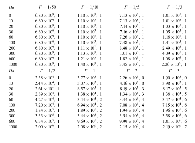
are listed in table 3 for practical reference. These data show that, for the case with
 $\varGamma =1/50$
, where the onset of convection is dominated by the geometrical confinement,
 $Ra_c$
remains nearly constant at
 $6.80\times 10^9$
.
3.2. Overview of flow structures
For a clearer understanding and distinction of the different regimes, we present flow visualisations at fixed
 $\textit{Ha}=300$
with varying
 $\varGamma$
in figure 5. It can be seen from figure 4(b) that the cases with
 $\textit{Ha}=300$
explore all the flow regimes ranging from the geometry-dominated regime to the wall-mode-dominated regime. To better visualise the internal flow structures, we show in figure 5(a)–(d) the velocity vector plots with half of the cylinder removed. In addition, the corresponding horizontal cross-sections of the contours of the normalised vertical velocity
 $U_z / \max {|U_z|}$
at
 $z=1/2$
are presented in figure 5(e)–(h). For the case of
 $\varGamma =1/20$
, which is located in the geometry-dominated regime, the flow exhibits the classical single-roll cellular structure (Shishkina Reference Shishkina2021; Zhang & Xia Reference Zhang and Xia2023; Ren et al. Reference Ren, Tao, Xia and Xie2024), associated with the azimuthal mode number
 $n=1$
(see figure 5
a,e). For the case of
 $\varGamma =1/10$
, which lies in the coupled regime without the formation of wall modes, the flow still maintains a single-roll cellular structure, not showing any significant difference from the geometry-dominated regime, as shown in figure 5(b, f). When
 $\varGamma =1/2$
, corresponding to the wall-mode developing regime, the onset pattern is also characterised by the
 $n=1$
mode, but with the velocity vectors concentrated near the sidewalls, indicating the occurrence of the wall modes. One may also notice that the flow in the core region of the cylindrical cell is weak (see figure 5
c). The difference between the flow pattern in the coupled regime and that in the wall-mode developing regime can be seen more clearly from the contour plots of the normalised vertical velocity shown in figures 5( f) and 5(g). Finally, in the wall-mode-dominated regime with
 $\varGamma =1$
, the flow exhibits a typical
 $n=2$
wall-mode structure, with no velocity vectors in the core region of the cylindrical cell (see figure 5
d,h). Note that the finer features, such as the typical two-layer structure of the wall modes, are too weak to be observed in these visualisations. We will give a quantitative analysis of the wall-mode structure based on the radial velocity profiles, which will be discussed in § 3.4.
Flow visualisations in different regimes at
 $\textit{Ha}=300$
with varying
 $\varGamma$
: (a,e) geometry-dominated regime,
 $\varGamma =1/20$
; (b, f) coupled regime,
 $\varGamma =1/10$
; (c,g) wall-mode developing regime,
 $\varGamma =1/2$
; (d,h) wall-mode-dominated regime,
 $\varGamma =1$
. In (a–d), half of the cylinder is removed to reveal the interior structure, where velocity vectors are indicated by arrows and colours represent normalised temperature fluctuations. In (e–h), the contours of the normalized vertical velocity
 $U_z/U_{z,max}$
at the horizontal cross-sections with
 $z=1/2$
are shown.

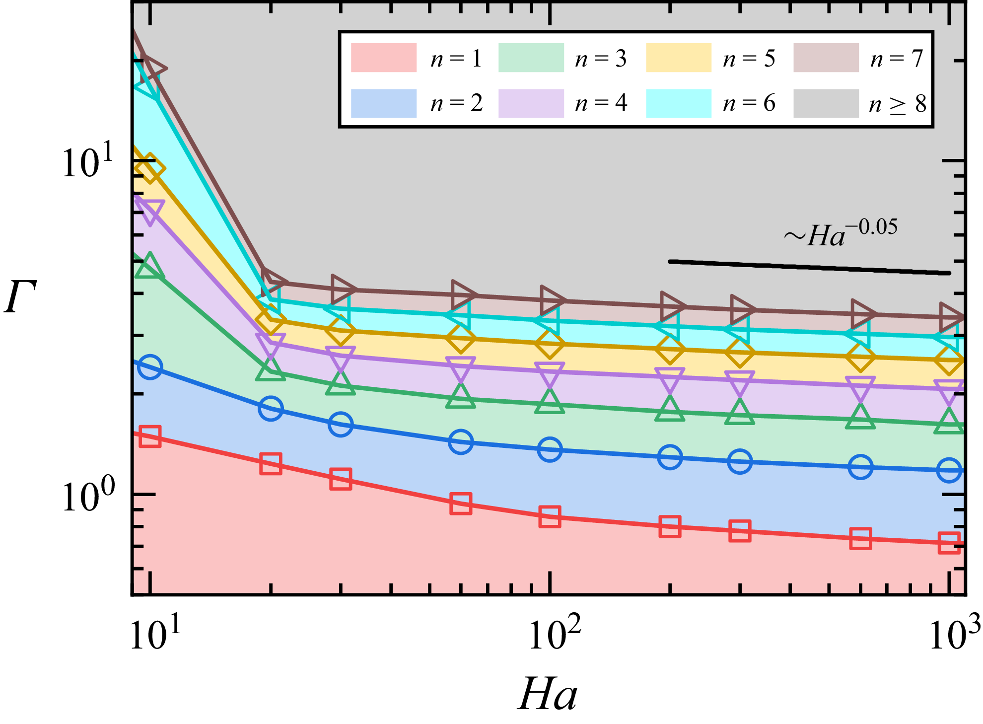
3.3. Azimuthal length scale
We study the azimuthal length scale of the flow in this subsection. The dimensionless azimuthal length scale
 $\ell _\theta$
is characterised by the mode number
 $n$
, which is shown in a
 $\varGamma -Ha$
phase space in figure 6. The symbols mark the transitional aspect ratio between successive
 $n$
. Note that the mode number here is not limited to wall modes. For example, no wall mode is observed for
 $\textit{Ha} \lesssim 20$
, but the flow has its
 $\ell _\theta$
. Due to the different flow structure with
 $\textit{Ha}$
, a noticeable change in the slope of the curves in figure 6 is observed near
 $\textit{Ha}= 20$
. For sufficiently large
 $\textit{Ha}$
,
 $n$
becomes weakly dependent on
 $\textit{Ha}$
. If a power-law fit to the transition points from
 $n=7 \rightarrow 8$
in the
 $100 \leqslant Ha \leqslant 1000$
range, one obtains
 $\varGamma \sim \textit{Ha}^{-0.05}$
, i.e. for a given
 $\varGamma$
, large
 $\textit{Ha}$
will result in a slight increase in
 $n$
, and the
 $\ell _\theta$
scales with
 $\textit{Ha}$
as
 $\textit{Ha}^{-0.05}$
. To study the effects of
 $\varGamma$
on
 $\ell _\theta$
, we focus on the case with
 $\textit{Ha} = 100$
. By fitting
 $n$
vs the
 $\varGamma$
corresponds to the minimum
 $Ra_c$
for a given
 $n$
, we obtain
 $n \approx 1.80 \varGamma ^{1.07}$
. This gives a mean azimuthal length scale
 $\ell _\theta = \pi D/(2n) \approx \pi /3.6$
, independent of
 $\varGamma$
. The observation suggests that, for a fixed
 $\textit{Ha}$
, with increasing
 $\varGamma$
, the typical azimuthal length scale of the wall modes remains unchanged and only its number increases.
The azimuthal mode number
 $n$
in the
 $\varGamma$
–
 $\textit{Ha}$
phase space. The symbols mark the transitional aspect ratio between successive
 $n$
. The black solid line with
 ${\sim} \textit{Ha}^{-0.05}$
is plotted as a line to guide the eye.

3.4. Radial length scales
Having obtained the azimuthal length scale, we then turn our attention to the dependence of the radial length scale
 $\ell _r$
on
 $\varGamma$
and
 $\textit{Ha}$
. Let us first focus on the case of
 $\textit{Ha}=100$
. Figure 7(a) plots the radial profile of the normalised vertical velocity
 $U_z^* = U_z / \max (|U_z|)$
for different
 $\varGamma$
. These profiles are taken at the centre of the upward wall-mode region. Note that the profiles of the downward region of the wall modes will yield similar profiles but with an opposite sign. The azimuthal wavenumber
 $n$
is also listed in the legend. The profiles with
 $n\geqslant 3$
for large
 $\varGamma$
almost coincide with each other, indicating
 $n$
should not affect the structure of the wall modes. When
 $\varGamma \lt 0.64$
, the profile shows a typical signature of the cellular structure observed without a magnetic field. As
 $\varGamma$
increases, the horizontal extent of the container becomes larger. But one observes that the distance of the location of maximum velocity relative to the sidewall
 $\delta _1$
converges toward a fixed location. This can be seen more clearly from the plot of
 $\delta _1$
vs
 $\varGamma$
shown in figure 7(b), where one observes that
 $\delta _1$
reaches a constant of 0.076 for large
 $\varGamma$
. We denote this constant as the first characteristic length scale
 $\ell _{r_1}$
of the wall modes. The intersection point of
 $\ell _{r_1}$
with
 $\delta _1$
is denoted as
 $\varGamma ^*_{1}$
(the red dash-dotted line), which is the minimum aspect ratio required for the wall modes to form. Figure 7(a) also shows that, when
 $\varGamma \geqslant 1.10$
, the typical two-layer structure of wall modes emerges. The velocity magnitude decays to zero rapidly toward the cell centre. The evolution of the distance of the location of the negative peak relative to the sidewall
 $\delta _2$
with
 $\varGamma$
is shown in figure 7(b). It can be seen that the second layer emerges only when
 $\varGamma$
is larger than a critical value denoted as
 $\varGamma ^*_2$
(the blue dash-dotted line). In addition,
 $\delta _2$
reaches a constant with increasing
 $\varGamma$
. We denote this constant as the second characteristic length scale
 $\ell _{r_2}$
of the wall modes.
(a) Radial profiles of the normalised vertical velocity
 $U_z / \max {|U_z|}$
for various
 $\varGamma$
at
 $\textit{Ha} = 100$
with
 $n$
being the azimuthal wavenumber. (b) Variation of the locations of the maximum positive (
 $\delta _1$
) and minimum negative (
 $\delta _2$
) vertical velocity profiles with
 $\varGamma$
for
 $\textit{Ha} = 100$
. The horizontal lines indicate the characteristic length scales of the two-layer structure,
 $\ell _{r_1}$
(red-dashed line) and
 $\ell _{r_2}$
(blue-dashed line). The vertical dashed lines mark the minimum
 $\varGamma$
required for the formation of each layer, denoted as
 $\varGamma ^*_1$
(red-dash-dotted line) and
 $\varGamma ^*_2$
(blue-dash-dotted line). (c) Dependence of
 $\ell_{r_1}$
and
 $\ell_{r_2}$
on
 $\textit{Ha}$
. The solid lines are power law fits to the data with
 $\ell_{r_1}=1.04Ha^{-0.56}$
and
 $\ell_{r_2}=4.94Ha^{-0.56}$
. The inset shows the ratio of the velocity amplitudes between the inner and outer layers as a function of
 $ \textit{Ha}$
. The solid line is a power law fit to the data with
 $-U_z(\ell_{r_2})/U_z(\ell_{r_1})=0.28Ha^{-0.23}$
. (d) Variation of
 $\varGamma ^*_1$
and
 $\varGamma ^*_2$
with
 $\textit{Ha}$
. The solid lines are power law fits to the data with
 $\varGamma_1^*=5.39 \textit{Ha}^{-0.58}$
and
 $\varGamma_2^*=9.07 \textit{Ha}^{-0.53}$
.

The dependence of radial length scales
 $\ell _{r_1}$
and
 $\ell _{r_2}$
on
 $\textit{Ha}$
is studied systematically, and the result is shown in figure 7(c). The data can be fitted by power laws, i.e.
 $\ell _1=1.04\textit{Ha}^{-0.56}$
and
 $\ell _2=4.94\textit{Ha}^{-0.56}$
. Thus, the two layers have similar dependence on
 $\textit{Ha}$
. In addition, the first layer is roughly 1/5 that of the second layer, and their ratio remains unchanged with increasing
 $\textit{Ha}$
. In the asymptotic analysis of Busse (Reference Busse2008) for a semi-infinite domain with free-slip top and bottom boundaries, a characteristic length scale proportional to
 $\textit{Ha}^{-1/2}$
was obtained, which is in good agreement with the present results. The slight deviation may be attributed to differences in the system configuration and boundary conditions. The strength of the two layers of the wall modes can be quantified by their vertical velocity magnitude. The ratio
 $-U_z(\ell _{r_2})/U_z(\ell _{r_1})$
is shown in the inset in figure 7(c). A power-law fit to the data yields
 $-U_z(\ell _{r_2})/U_z(\ell _{r_1})=0.28\textit{Ha}^{-0.23}$
. The negative scaling exponent suggests that the second layer’s structure becomes increasingly weaker compared with that of the first layer as the magnetic field becomes stronger suggesting that it will become much more difficult to measure the two-layer structure for high
 $\textit{Ha}$
number magnetoconvection.
To elucidate the formation mechanism of wall modes in confined geometry, we study the dependence of
 $\varGamma ^*_1$
and
 $\varGamma ^*_2$
on
 $\textit{Ha}$
as shown in figure 7(d). The data can be fitted by power laws, i.e.
 $\varGamma ^*_1=5.39\textit{Ha}^{-0.58}$
and
 $\varGamma ^*_2=9.07\textit{Ha}^{-0.53}$
, respectively. Note that we have determined the critical aspect ratio
 $\varGamma _{c_2}(Ha)$
when the wall modes start to emerge based on
 $Ra_c$
in figure 4(b). As the analysis based on length scale also shows a similar physical process, i.e.
 $\varGamma ^*_1(Ha)$
marks the point when the velocity profile shows signatures of wall modes, one expects that
 $\varGamma _{c_2}(Ha)$
should be close to
 $\varGamma ^*_1(Ha)$
. We have tested this and found it is indeed the case. This agreement on the emerging point of wall modes suggests a strong connection between
 $Ra_c$
and flow structures in magnetoconvection. We also note that
 $\varGamma ^*_2$
is smaller than
 $\varGamma _{c_3}$
, indicating that, although the second layer’s structure emerges at
 $\varGamma ^*_2$
, a further increase in
 $\varGamma$
is required for the wall modes to become fully developed, i.e. the vertical velocity profile of the wall modes do not change with
 $\varGamma$
, and
 $Ra_{c,w}$
becomes independent of
 $\varGamma$
.
4. Conclusion and outlook
In summary, we have studied the onset of wall modes in confined magnetoconvection with a vertical magnetic field using LSA. Our study revealed dynamically how wall modes emerge and evolve with decreasing geometrical confinement, characterised by the aspect ratio
 $\varGamma$
of the convection cell. A phase diagram of the dominating factors that determine the critical Rayleigh number
 $Ra_c$
for the onset of convection in the
 $\varGamma -Ha$
phase space is given. For
 $\varGamma \lt \varGamma _{c_1} = 1.21 \textit{Ha}^{-0.48}$
,
 $Ra_c$
is mainly determined by the geometrical confinement with
 $Ra_c = 1090 \varGamma ^{-4.0}$
. For
 $\varGamma _{c_1} \leqslant \varGamma \lt \varGamma _{c_2} = 4.07 \textit{Ha}^{-0.53}$
, no wall modes form and
 $Ra_c$
depends on both the strength of confinement and magnetic field. For
 $\varGamma _{c_2}\leqslant \varGamma \lt \varGamma _{c_3}=0.99 \textit{Ha}^{-0.10}$
, wall modes emerge and
 $Ra_c$
drops below the bulk onset; for
 $\varGamma \geqslant \varGamma _{c_3}$
, wall modes become fully developed and their onset Rayleigh number
 $Ra_{c,w} \approx 65 \textit{Ha}^{1.5}$
, independent of
 $\varGamma$
.
The structure of the wall modes is studied in detail based on their radial profiles of the vertical velocity. It is found that, for a given
 $\textit{Ha}$
, the first layer of the wall modes emerges when
 $\varGamma \geqslant 5.39\textit{Ha}^{-0.58}$
. The two-layer structure of wall modes forms when
 $\varGamma \geqslant 9.07\textit{Ha}^{-0.53}$
. The fully developed wall mode emerges when
 $\varGamma \geqslant 0.99 \textit{Ha}^{-0.10}$
. This fully developed state is characterised by their vertical velocity profiles do not change with
 $\varGamma$
and
 $Ra_{c,w}$
is independent of
 $ \varGamma $
. We further showed that the relative magnitude of the two-layer structure decreases with
 $\textit{Ha}$
, indicating that it will be difficult to capture the second layer of the wall modes for large
 $\textit{Ha}$
. These findings provide practical guidelines for experimental and numerical studies of the wall-mode dynamics. Finally, we remark that although the onset of a wall mode is independent of
 $\textit{Pr}$
, once the flow is initiated, its evolution with
 $Ra/Ra_{c,w}$
exhibits a strong dependence on
 $\textit{Pr}$
. Thus, it will be worthwhile to study the effects of
 $\textit{Pr}$
on the interaction of wall modes and bulk convection.
Acknowledgements
We thank the anonymous referees for the helpful comments.
Funding
This work is supported by the National Natural Science Foundation of China under grant Nos. 12422209, 12595303, a XJTU young talent support plan and the Fundamental Research Funds for the Central Universities under grant number xtr042024012.
Declaration of interests
The authors report no conflict of interest.
Appendix A. Details on reducing the problem to an eigenvalue problem
For axisymmetric modes (
 $n=0$
), after applying the Galerkin method, we have
 \begin{equation} \left ( \begin{matrix} \bar { \bar {M}}_{11} & \bar { \bar {M}}_{12} \\ Ra\bar { \bar {M}}_{21} & \bar { \bar {M}}_{22} \end{matrix} \right ) \left ( \begin{matrix} \bar {H} \\ \bar {A} \end{matrix} \right ) =0, \end{equation}
where a single overbar denotes a vector, a double overbar denotes a matrix and
 \begin{equation} \bar { \bar {M}}_{11}=\int _{V} T_{\textit{jm}} \boldsymbol{\nabla }^2 T_{il} \,{\rm d}V ;\, \bar { \bar {M}}_{12}=\int _{V} T_{\textit{jm}} \hat {\boldsymbol{e}}_{\boldsymbol{z}} \boldsymbol{\cdot }\boldsymbol{U}_{il} \,{\rm d}V ;\, \bar { \bar {M}}_{21}=\int _{V} \hat {\boldsymbol{e}}_{\boldsymbol{z}} \boldsymbol{\cdot }\boldsymbol{U}_{\textit{jm}} T_{il} \,{\rm d}V , \end{equation}
 \begin{equation} \bar { \bar {M}}_{22}=\int _{V} \boldsymbol{U}_{\!\textit{jm}}\boldsymbol{\cdot }\boldsymbol{\nabla }^2 \boldsymbol{U}_{il}-\textit{Ha}^2 U_{r,jm} U_{r,il} \,{\rm d}V . \end{equation}
The vectors
 $\bar {H}$
can be eliminated from (A1) to reduce the problem to standard eigenvalue form
 \begin{equation} \left ( \bar { \bar {M}}_{22}^{-1} \bar { \bar {M}}_{21} \bar { \bar {M}}_{11}^{-1} \bar { \bar {M}}_{12}-\frac {\bar { \bar {I}}}{Ra} \right )\bar {A}=0. \end{equation}
For asymmetric modes (
 $n\gt 0$
), we have
 \begin{equation} \left ( \begin{matrix} \bar { \bar {M}}_{11} & \bar { \bar {M}}_{12} & 0 & 0 \\ Ra\bar { \bar {M}}_{21} & \bar { \bar {M}}_{22} & \bar { \bar {M}}_{23} & \bar { \bar {M}}_{24} \\ 0 & \bar { \bar {M}}_{32} & \bar { \bar {M}}_{33} & \bar { \bar {M}}_{34} \\ 0 & \bar { \bar {M}}_{42} & \bar { \bar {M}}_{43} & \bar { \bar {M}}_{44} \end{matrix} \right ) \left ( \begin{matrix} \bar {H} \\ \bar {B} \\ \bar {D} \\ \bar {G} \end{matrix} \right ) =0 , \end{equation}
where
 \begin{equation} \bar { \bar {M}}_{11}=\int _{V} T_{\textit{jm}} \boldsymbol{\nabla }^2 T_{il} \,{\rm d}V ;\, \bar { \bar {M}}_{12}=\int _{V} T_{\textit{jm}} \hat {\boldsymbol{e}}_{\boldsymbol{z}} \boldsymbol{\cdot }\boldsymbol{U}_{il}^{(1)} \,{\rm d}V , \end{equation}
 \begin{equation} \bar { \bar {M}}_{21}=\int _{V} \hat {\boldsymbol{e}}_{\boldsymbol{z}} \boldsymbol{\cdot }\boldsymbol{U}_{\textit{jm}}^{(1)} T_{il} \,{\rm d}V ;\, \bar { \bar {M}}_{22}=\int _{V} \boldsymbol{U}_{\textit{jm}}^{(1)} \boldsymbol{\cdot }\boldsymbol{\nabla }^2 \boldsymbol{U}_{il}^{(1)}-\textit{Ha}^2 U^{(1)}_{\theta ,jm} U^{(1)}_{\theta ,il} \,{\rm d}V , \end{equation}
 \begin{equation} \bar { \bar {M}}_{23}=\int _{V} \boldsymbol{U}_{\textit{jm}}^{(1)} \boldsymbol{\cdot }\boldsymbol{\nabla }^2 \boldsymbol{U}_{il}^{(2)}-\textit{Ha}^2 U^{(1)}_{\theta ,jm} U^{(2)}_{\theta ,il} \,{\rm d}V , \end{equation}
 \begin{equation} \bar { \bar {M}}_{24}=\int _{V} -\textit{Ha}^2 U^{(1)}_{\theta ,jm} \left ( \boldsymbol{\nabla } \phi _{il}\times \hat {\boldsymbol{e}}_{\boldsymbol{z}} \right )_{\theta } \,{\rm d}V , \end{equation}
 \begin{equation} \bar { \bar {M}}_{32}=\int _{V} \boldsymbol{U}_{\textit{jm}}^{(2)} \boldsymbol{\cdot }\boldsymbol{\nabla }^2 \boldsymbol{U}_{il}^{(1)}-\textit{Ha}^2 U^{(2)}_{\theta ,jm} U^{(1)}_{\theta ,il} \,{\rm d}V , \end{equation}
 \begin{equation} \bar { \bar {M}}_{33}=\int _{V} \boldsymbol{U}_{\textit{jm}}^{(2)} \boldsymbol{\cdot }\boldsymbol{\nabla }^2 \boldsymbol{U}_{il}^{(2)}-\textit{Ha}^2 \big ( U^{(2)}_{r,jm} U^{(2)}_{r,il}+U^{(2)}_{\theta ,jm} U^{(2)}_{\theta ,il} \big ) \,{\rm d}V , \end{equation}
 \begin{equation} \bar { \bar {M}}_{34}=\int _{V} -\textit{Ha}^2 \big ( U^{(2)}_{r,jm} \big ( \boldsymbol{\nabla } \phi _{il}\times \hat {\boldsymbol{e}}_{\boldsymbol{z}} \big )_{r} + U^{(2)}_{\theta ,jm} \big ( \boldsymbol{\nabla } \phi _{il}\times \hat {\boldsymbol{e}}_{\boldsymbol{z}} \big )_{\theta } \big ) \,{\rm d}V, \end{equation}
 \begin{equation} \bar { \bar {M}}_{42}=\int _{V} \phi _{\textit{jm}} \boldsymbol{\nabla } \boldsymbol{\cdot }\big ( U^{(1)}_{\theta ,il} \hat {\boldsymbol{e}}_{\boldsymbol{r}} \big ) \,{\rm d}V;\, \bar { \bar {M}}_{43}=\int _{V} \phi _{\textit{jm}} \boldsymbol{\nabla } \boldsymbol{\cdot }\big ( U^{(2)}_{\theta ,il} \hat {\boldsymbol{e}}_{\boldsymbol{r}} - U^{(2)}_{r,il} \hat {\boldsymbol{e}}_{\boldsymbol{\theta }} \big ) \,{\rm d}V, \end{equation}
 \begin{equation} \bar { \bar {M}}_{44}=\int _{V} -\phi _{\textit{jm}} \boldsymbol{\nabla }^2\phi _{il} \,{\rm d}V. \end{equation}
The vectors
 $\bar {H}$
,
 $\bar {D}$
and
 $\bar {G}$
in (A5) can be eliminated, then the standard eigenvalue formulation is obtained, i.e.
 \begin{equation} \left ( \big ( \bar { \bar {M}}_{22}-\bar { \bar {M}}_{D}-\bar { \bar {M}}_{G} \big )^{-1} \bar { \bar {M}}_{21} \bar { \bar {M}}_{11}^{-1}\bar { \bar {M}}_{12}-\frac {\bar { \bar {I}}}{Ra} \right )\bar {B}=0, \end{equation}
where
 \begin{equation} \bar { \bar {M}}_{D}=\bar { \bar {M}}_{23}(\bar { \bar {M}}_{43}-\bar { \bar {M}}_{44}\bar { \bar {M}}_{34}^{-1}\bar { \bar {M}}_{33})^{-1}(\bar { \bar {M}}_{42}-\bar { \bar {M}}_{44}\bar { \bar {M}}_{34}^{-1}\bar { \bar {M}}_{32}), \end{equation}
 \begin{equation} \bar { \bar {M}}_{G}=\bar { \bar {M}}_{24}(\bar { \bar {M}}_{44}-\bar { \bar {M}}_{43}\bar { \bar {M}}_{33}^{-1}\bar { \bar {M}}_{34})^{-1}(\bar { \bar {M}}_{42}-\bar { \bar {M}}_{43}\bar { \bar {M}}_{33}^{-1}\bar { \bar {M}}_{32}). \end{equation}
Then, for each
 $n$
and a given
 $\varGamma$
, a series of Rayleigh numbers
 $Ra$
can be solved from the corresponding eigenvalue equation with the minimum
 $Ra$
denoted as the critical Rayleigh number
 $Ra_{c,n}$
for the
 $n$
-mode instability. The associated onset flow pattern can also be determined accordingly. Finally, the overall onset Rayleigh number
 $Ra_{c}$
is defined as the minimum of
 $Ra_{c,n}$
over all azimuthal modes
 $n$
, as discussed in § 3.1.