


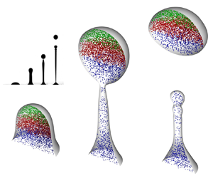



1. Introduction
Various modes of fluid fragmentation inherent to foliar disease transmission have been linked to the average wetting dominating most crop leaves (Gilet & Bourouiba Reference Gilet and Bourouiba2014, Reference Gilet and Bourouiba2015, Reference Gilet and Bourouiba2017). One such mode is the inertial detachment: upon impact from rain, irrigation or dew drops, the motion of a compliant leaf locally transfers its impulse to a sessile contaminated drop residing on it. The contaminated drop forms a ligament that detaches from the leaf, ejecting secondary droplets through end-pinching. Such resulting fragmentation of the sessile contaminated drop is particularly interesting in this application domain for its ability to produce highly contaminated ejected droplets that do not undergo any dilution and typically produce a distinct primary tip drop. Indeed, little to no mixing between the impacting and the contaminated drop occurs from this process. Figure 1, adapted from Gilet & Bourouiba (Reference Gilet and Bourouiba2015), shows an image sequence of drop inertial detachment driven by the flexural motion of a compliant leaf, upon raindrop-like impact.
Inertial detachment from a compliant leaf induced by raindrop impact. Images recorded 62.5 to 122.5 ms after drop impact. A scale bar of 5 mm is given. Here, the associated Bond number according to (2.8a,b) is estimated as  $\textit {Bo} \approx 8$. The inset shows a schematic. Images adapted with permission from Gilet & Bourouiba (Reference Gilet and Bourouiba2015).

Fragmentation from liquid column disintegration is also relevant for a wide range of engineering, physical and biological systems and applications involving impacts of drops on surfaces or films/pools, with end-pinching of ligaments, or their merger shaping, in part or fully, the distribution of ejected droplets of varying sizes and speeds (Qian & Law Reference Qian and Law1997; Villermaux & Bossa Reference Villermaux and Bossa2011; Wang & Bourouiba Reference Wang and Bourouiba2018, Reference Wang and Bourouiba2021; Lejeune, Gilet & Bourouiba Reference Lejeune, Gilet and Bourouiba2018). Such applications include spray coating, agricultural irrigation, fuel combustion (Yarin Reference Yarin2006; Villermaux Reference Villermaux2007), microfluidic and electronic systems (Sarobol et al. Reference Sarobol, Cook, Clem, Keicher, Hirschfeld, Hall and Bell2016), functional materials printing (Derby Reference Derby2010), bioinks for 3D printing (Gopinathan & Noh Reference Gopinathan and Noh2018) and more generally disease transmission, from mucosalivary fluid fragmentation relevant for respiratory disease transmission to bursting bubbles for waterborne pathogens in addition to the fragmentation of sessile pathogen-laden drops on leaves relevant for foliar disease transmission between plants outlined above (Poulain & Bourouiba Reference Poulain and Bourouiba2018, Reference Poulain and Bourouiba2019; Bourouiba Reference Bourouiba2021a,Reference Bourouibab).
Inertial detachment is also interesting as a fundamental fragmentation process on its own merit, as the asymmetric stretching under impulsive axial forcing shapes the fragmentation of the initially sessile drop. It is well known that elongated and slender liquid ligaments undergo fragmentation due to surface-tension-induced instability. The normal mode related growth of interface perturbation is typically attributed to a Rayleigh–Plateau (R–P) type instability (Plateau Reference Plateau1873; Rayleigh Reference Rayleigh1878; Eggers Reference Eggers1993, Reference Eggers1995). The R–P instability assumes an infinitely long cylindrical fluid column. On the other hand, Stone, Bentley & Leal (Reference Stone, Bentley and Leal1986) and Stone & Leal (Reference Stone and Leal1989) showed that end-pinching prior to the manifestation of the R–P instability can be the driver of fragmentation for contracting viscous filaments of finite length. Such unsteady, non-modal fragmentation motivated experimental and numerical studies on recoiling filaments and end-pinching of symmetrical ligament breakup (Schulkes Reference Schulkes1996; Notz & Basaran Reference Notz and Basaran2004; Castrejón-Pita, Castrejón-Pita & Hutchings Reference Castrejón-Pita, Castrejón-Pita and Hutchings2012). Moreover, the effect of axial stretching on the stability of an inertial jet was also first discussed analytically by Frankel & Weihs (Reference Frankel and Weihs1985), and later extended by Henderson et al. (Reference Henderson, Segur, Smolka and Wadati2000). The breakup of liquid bridges formed in extensional flows was also further investigated (Slobozhanin & Perales Reference Slobozhanin and Perales1993; Gaudet, McKinley & Stone Reference Gaudet, McKinley and Stone1996; Marmottant & Villermaux Reference Marmottant and Villermaux2004; Vincent, Duchemin & Villermaux Reference Vincent, Duchemin and Villermaux2014). These studies established that the strength of inertial acceleration, e.g. gravity, relative to surface tension, as measured by the Bond number,  $Bo$, and the liquid–solid contact dynamics determine the stability regimes of an inviscid bridge. However, the findings of this large body of work is not directly applicable to the end-pinching of elongated drops we are concerned about herein, where the asymmetry of the stretching imposed by axial forcing and contact dynamics at the fluid–structure interface are major distinctions from prior work on ligament breakup.
End pinching was also treated in detail for pendant drops, for example via equilibrium analysis (e.g. Padday, Pitt & Tabor Reference Padday, Pitt and Tabor1973; Boucher & Kent Reference Boucher and Kent1978). Although unsteady evolution of pendent drops was captured subsequently (e.g. via high-speed imaging, Peregrine, Shoker & Symon Reference Peregrine, Shoker and Symon1990) catalysing numerous non-equilibrium theoretical and numerical investigations (e.g. Eggers & Dupont Reference Eggers and Dupont1994; Schulkes Reference Schulkes1994; Brenner et al. Reference Brenner, Eggers, Joseph, Nagel and Shi1997; Wilkes, Phillips & Basaran Reference Wilkes, Phillips and Basaran1999; Ambravaneswaran, Wilkes & Basaran Reference Ambravaneswaran, Wilkes and Basaran2002), dripping flows exiting nozzles remained generally the focus of these studies. Such flows differ from the end-pinching from inertial detachment of a sessile drop we are concerned about here where contact-line wetting and limited mass constraint are essential ingredients of the fragmentation and secondary ejected daughter drop formation.
In this article, we address the following questions:
(i) When does a sessile drop first detach/fragment from its supporting substrate under inertial forcing? And after fragmentation, what is the amount of the liquid content released?
(ii) What are the roles of the imposed inertial force, surface tension and surface wetting in the selection of the fragments? And as the drop deforms, what are the dominant physical mechanisms that cause primary fragmentation?
(iii) How do these mechanisms determine the detachment time and the size of primary daughter fragment/droplet release?
(iv) What is the role of the solid–liquid contact line in shaping the fragmentation of the primary drop?
(v) Finally, returning to our original application of interest, and having validated our modelling of the inertial detachment end-pinching against experiments, what can we learn about the distribution of organisms of various wetting properties (e.g. hydrophobic spores vs wetting neutrally buoyant bacteria) in the primary ejected drop vs secondary droplets?
To address these questions, we combine experimental and theoretical approaches also with direct numerical simulations (DNS) of the liquid–gas two-phase Navier–Stokes equations incorporating two different dynamic models for the liquid–solid contact. We begin in § 2 with a reduced experimental set-up that mimics the drop detachment flow observed on plant leaves. This involves first depositing a sessile drop on stationary plate substrates of different affinities for water, and then impulsively imposing a constant acceleration to the plate–drop system in the direction of gravity, while monitoring the consequent drop deformation and fragmentation and controlling for lateral vibration.
In response to (i) we find that the original sessile drop elongates into a ligament and subsequently breaks under inertial acceleration; surprisingly, however, the breakup time and size of the first ejected drop at the ligament tip become insensitive to both the Bond number and the equilibrium liquid–solid contact angle as the Bond number increases. In response to (ii) and (iii) using the DNS (introduced in § 2.3), we examine the role of capillarity and inertia in isolation, revealing the dominant factors that control the chain of fragmentation (§ 3). We develop asymptotic theories in the large Bond number limit (§ 3), leveraging the extreme aspect ratios of the drop/ligament during different stages of the deformation, i.e. thin film vs slender jet. In particular, we capture the effect of surface tension via geometrical arguments and propose a ‘lollipop’ structure for the ligament at its pinch-off time. The ‘lollipop’ reduced theoretical model captures the experimental and DNS results well. In response to (iii) and (iv), we identify (§ 3.5) that the error in prediction on the primary drop size and breakup time is caused by the contact dynamics, which has weak, but lasting effects on the end-pinching dynamics. Moreover, correction to the leading-order theory can be achieved by modifying the simple contact model used in the DNS and asymptotic theory. Having validated the numerical and theoretical model against experiments, in response to (v) (§ 4) we examine how reduced analogue pathogens/contaminants of different wetting properties distribute in the fragments, i.e. primary drop and satellite droplets. We conclude in § 5.
2. Inertial detachment analogue experiments and physical picture
In its original discovery by Gilet & Bourouiba (Reference Gilet and Bourouiba2014, Reference Gilet and Bourouiba2015, Reference Gilet and Bourouiba2017), inertial detachment fragmentation (e.g. figure 1) was associated with average wetting surfaces leading to retention of drops on the surface via hysteresis. The initially sessile drops were observed to be accelerated via the impact of other drops (e.g. rain or dew), imparting inertia to the leaf that, in turn, accelerates the sessile drops. To simplify the study of this fragmentation process, we adopt an analogue experimental set-up with a sessile drop on a plate (figure 2) and imparting axial extension in the same direction as gravity. Our simplification enables us to derive insights into the fundamental mechanisms driving this fragmentation process. We first introduce the details of that experimental analogue system, and then discuss the key results of the inertial detachment.
(a) Experimental schematic. The substrate is impulsively accelerated at  $t=0^+$ by the spring at constant accelerating
 $a$ in the same direction as gravity. (b) Axisymmetric drop geometry under two-dimensional (2-D) cylindrical coordinate system. Here,
 $u,w$ are the flow velocity components in the plate-stationary frame;
 $\alpha$ is the magnitude of inertial acceleration.

2.1. Experimental method
The experimental set-up is shown schematically in figure 2(a) where a sessile water drop of volume  $V$ is deposited on a locked, stationary horizontal plate. From below, the substrate is attached to a spring system in extension. At time
 $t=0^+$, the spring is released, imposing a normal (downward) acceleration
 $a$ on the plate. The acceleration
 $a$ is maintained close to constant in each experiment with a sufficiently long extension of the spring. Its value is calculated and monitored for each experiment through image processing of the high-speed recordings. The impulsive translation motion of the substrate results in unsteady, axisymmetric deformation of the drop that is also recorded via high-speed imaging in side view at 2000 frames per second. The distance between the fixed camera and the moving drop is
 $O(100)$ larger than the drop's observed vertical displacement, ensuring negligible perspective distortion in imaging.
Focusing on the intermediate wetting conditions described in Gilet & Bourouiba (Reference Gilet and Bourouiba2015), this study uses polymethyl methacrylate (PMMA) as a substrate as it is comparatively hydrophobic. As a comparison and for reference we also add double-frosted microscope slides (microslides) that are comparatively more hydrophilic. The static contact angle between the drop and substrate given by PMMA and microslides are  $\theta _c=60^\circ$ and
 $\theta _c=19^\circ$, respectively (illustrated in figure 2b at
 $t=0$). For each substrate, a series of experiments is conducted with varying plate acceleration
 $a$ and sessile drop volume
 $V$ in ranges listed in table 1. Standard properties of water under room temperature and atmospheric pressure are taken for density
 $\rho$, surface tension
 $\sigma$ and dynamic viscosity
 $\mu$.
Experimental parameters. Here,  $\theta _c$ is drop equilibrium contact angle,
 $a$ is the plate acceleration,
 $V$ is the drop initial volume (in microlitres) with measurement error of 1 %–5 % for the pipettes and volumes used,
 ${\textit {Bo}}$ and
 ${\textit {Re}}$ are, respectively, the inertial Bond and the Reynolds numbers defined in (2.8a,b) and
 ${\textit {Oh}}=\sqrt {{\textit {Bo}}}/{\textit {Re}}$ is the Ohnesorge number. Given the large values of
 ${\textit {Re}}$ (and small values of
 ${\textit {Oh}}$), viscous effects are negligible.

2.2. Physical picture and non-dimensional characterization
Given the axisymmetric nature of the inertial detachment about the vertical axis parallel to the acceleration, we consider a two-dimensional cylindrical coordinate system of unit vectors  $\hat {\boldsymbol {r}}$ and
 $\hat {\boldsymbol {z}}$ co-moving with the substrate. The origin is taken to be at the centre of the sessile drop–substrate contact circle, as shown in figure 2(b).
2.2.1. Initial shape of the sessile drop
By choosing the length scale
 \begin{equation} R_{eq}=\left(\frac{3V}{4{\rm \pi}}\right)^{1/3}, \end{equation}
that gives the radius of an equivalent sphere of the same volume  $V$, the initial shape of the drop can be characterized by the dimensionless Young–Laplace equation (Lubarda & Talke Reference Lubarda and Talke2011)
 \begin{equation} \frac{1}{h_0(1+h_0'^2)^{1/2}}-\frac{h_0''}{(1+h_0'^2)^{3/2}}={-}2h_0''(L_0)+G(L_0-z), \end{equation}
where  $h_0(z)\equiv h(z,t=0^-)$ is the initial profile of the drop radius,
 $h_0'$ and
 $h_0''$ are its first and second derivatives with respect to
 $z$,
 $L_0$ is the initial height with
 $h_0(L_0)=0$ and
 \begin{equation} G = \frac{\rho g R_{eq}^2}{\sigma} \end{equation}
is the Bond number based on gravitational acceleration  $g$. The associated boundary condition
 \begin{equation} h_0'(0)={-}\cot\theta_c, \end{equation}
involves the equilibrium contact angle  $\theta _c$ that is a property of the substrate (table 1). Note that, in the
 $G\to 0$ limit, solution to (2.2) for
 $h_0(z)$ yields a spherical cap, as expected.
2.2.2. Drop evolution upon substrate acceleration
For  $t>0$, in the plate's reference frame, the drop is subject to both gravity and an inertial force due to the plate's acceleration, giving a net body force
 $\rho \alpha \hat {\boldsymbol {z}}$ where
 \begin{equation} \alpha = a-g , \end{equation}
is the effective acceleration. We subsequently default to the inertial velocity and time references
 \begin{equation} U_\alpha=\sqrt{\alpha R_{eq} },\quad T_\alpha=\sqrt{\frac{R_{eq}}{\alpha}}, \end{equation}
so the drop's flow through quiescent ambient air of negligible density and viscosity is governed by the non-dimensional Navier–Stokes equations, with pressure non-dimensionalized by  $\sigma /R_{eq}$, the capillary pressure

where  $\boldsymbol {u}=u\hat {\boldsymbol {r}}+w\hat {\boldsymbol {z}}$ is the velocity vector,
 $p$ is pressure,
 $\kappa$ is surface curvature,
 $\hat {\boldsymbol {n}}$ is the unit normal,
 $\delta _s$ is the surface Dirac
 $\delta$-distribution concentrated on the interface (Popinet Reference Popinet2018) and
 \begin{equation} {\textit{Bo}} \equiv \frac{\rho \alpha R_{eq}^2}{\sigma} = \frac{\alpha}{g}G,\quad {\textit{Re}} = \frac{\rho \alpha^{1/2}R_{eq}^{3/2}}{\mu} , \end{equation}
are the acceleration-based Bond number and Reynolds number, respectively. It is also convenient here to define the Ohnesorge number  ${\textit {Oh}}\equiv \mu /\sqrt {\rho \sigma R_{eq}}=\sqrt {{\textit {Bo}}}/{\textit {Re}}$ that directly compares viscous and surface tension effects. Finally, evolution of the profile
 $h(z,t)$ of the drop radius follows the kinematic condition
 \begin{equation} \left[\frac{\partial{h}}{\partial t}+w \frac{\partial h}{\partial z}\right]_{r=h}=u|_{r=h}. \end{equation}
2.2.3. Characteristic scales: inertial vs capillary scales
With an appropriate model for the contact dynamics prescribed at  $z=0$ (discussed in § 2.3), we have obtained a closed description for the drop under inertial acceleration for all
 $t\geq 0$. This system is governed by four dimensionless parameters: the contact angle
 $\theta _c$, gravitational Bond number
 $G$ (or equivalently, the acceleration ratio
 $\alpha /g$), the inertial Bond number
 ${\textit {Bo}}$ and the Reynolds number
 ${\textit {Re}}$. Ranges of
 ${\textit {Bo}}$ used in the experiments are given in table 1, whereas typical values of
 ${\textit {Re}}$ are of
 $O(10^{2-4})$. Therefore, the inviscid flow assumption is reasonable, until ligament pinch-off is approached (Lister & Stone Reference Lister and Stone1998). We will also focus on results obtained for small
 $G$ where gravitational effects on the initial drop shape and thus early-stage motion are small.
The competition between inertial acceleration and capillarity due to surface tension is a key mechanism that drives the drop deformation, therefore it is instructive to also introduce the dimensional capillary wavelength  $\varLambda$, time
 $T_\sigma$ and velocity
 $U_\sigma$ units
 \begin{equation} \varLambda = \sqrt{\frac{\sigma}{\rho \alpha}},\quad T_\sigma = \sqrt{\frac{\rho R_{eq}^3}{\sigma}},\quad U_\sigma = \alpha\sqrt{\frac{\rho R_{eq}^3}{\sigma}}. \end{equation}
Particularly,  $U_\sigma$ measures the change of speed generated by the imposed acceleration
 $\alpha$ over the capillary time scale
 $T_\sigma$. Under the inertial references (2.1) and (2.6a,b), these become
 \begin{equation} \lambda \equiv \frac{\varLambda}{R_{eq}}= \frac{1}{\sqrt{{\textit{Bo}}}},\quad t_\sigma \equiv \frac{T_\sigma}{T_\alpha} = \sqrt{{\textit{Bo}}},\quad u_\sigma \equiv \frac{U_\sigma}{U_\alpha} = \sqrt{{\textit{Bo}}}. \end{equation}
We henceforth denote  $\tau =t/\sqrt {{\textit {Bo}}}$ for rescaled physical dimensional time in capillary units, while
 $t$ is our default time non-dimensionalized by the inertial time scale
 $T_{\alpha }$ from (2.6a,b).
2.3. Methods for direct numerical simulations
2.3.1. Numerical framework and additional non-dimensional parameters
According to the framework given in § 2.2, the drop detachment experiments are also simulated numerically to further our understanding of the fragmentation mechanism that is critical for disease transmission applications. The key numerical methods are explained next.
We adopt Basilisk (Popinet Reference Popinet2009, Reference Popinet2015, Reference Popinet2018) and solve the axisymmetric incompressible two-phase Navier–Stokes equations with surface tension for the air–liquid system. Simulations of high density ratios like air–water and non-negligible inertia are numerically challenging, hence we employ the momentum-conserving volume-of-fluid (VoF) scheme (Arrufat et al. Reference Arrufat, Crialesi-Esposito, Fuster, Ling, Malan, Pal, Scardovelli, Tryggvason and Zaleski2021). This is particularly necessary for high  ${\textit {Bo}}$. Therein, the equations of motion for air, a counterpart of (2.7), are coupled and introduce ratios for density and dynamic viscosity:
 $\rho _a/\rho$ and
 $\mu _a/\mu$, between air (subscript
 $_a$) and water. These add to existing list of control parameters of the numerical system:
 $\theta _c$,
 ${\textit {Bo}}$,
 $G$ and
 ${\textit {Oh}}$.
2.3.2. Numerical model with constant contact-angle model
One challenge on the numerical modelling is the appropriate capture of the liquid–solid contact line dynamics. This turns out to be important, as discussed hereafter, to capture the tip and foot breakups. We start with a no-slip boundary condition at the wall along with a constant grid-scale contact angle as a first-order approximation. We subsequently develop a different numerical model in Appendix G where the constant angle approximation is relaxed. Unless otherwise stated, DNS results presented in the rest of this manuscript are obtained using the constant contact-angle model.
Regarding the first no-slip model, it has a force singularity at the contact line (Huh & Scriven Reference Huh and Scriven1971), which is handled in the VoF formulation using an implicit numerical slip (Afkhami, Zaleski & Bussmann Reference Afkhami, Zaleski and Bussmann2009). Specifically, we consider the standard water and air conditions, and simulate sessile drops of fixed initial volume  $56.5\,\mathrm {\mu }{\rm l}$ and therefore constant
 $G=0.755$ and
 $Oh=2.18\times 10^{-3}$ (comparable to the experimental values reported in table 1). The value of
 ${\textit {Bo}}$ is subsequently varied by changing
 $\alpha /g$. The case corresponding to
 $\theta _c = 60^\circ$ is extensively studied. The range of
 ${\textit {Bo}}$ in simulation is varied from 1.5 to 12. For
 $\theta _c = 60^\circ$, below the value of
 ${\textit {Bo}}=1.5$, fragmentation is suppressed.
2.4. Elongation and fragmentation of the sessile drop
2.4.1. The unstable breakup regime
Upon plate release, the initial sessile drop elongates vertically forming a ligament while its foot remains in contact with the substrate. For sufficiently large drop volume  $V$ and effective acceleration
 $\alpha$, necking occurs near the ligament tip as well as its foot, which ultimately leads to breakup and partial ejection of the sessile drop volume. A typical sequence of drop deformation is shown in figure 3(a i–a v), where (a i) gives the initial shape; (a ii) shows ligament formation; (a iii) and (a iv) respectively depict tip and foot pinch-off when the ligament breaks, ejecting secondary drops/ligaments from the original sessile drop; and finally (a v) illustrates that, after the foot pinch-off, the detached ligament further fragments into multiple satellite droplets. We will show in Appendix A that the order of tip and foot breakup depends on the Bond number
 ${\textit {Bo}}$.
(a) Successive temporal sequence of a drop undergoing inertial detachment and fragmentation. Experiment conducted with a PMMA substrate ( $\theta _c=60^\circ$), and with acceleration ratio
 $\alpha /g=4.2$ and drop initial volume
 $V=80\,\mathrm {\mu }\text {l}$. A dashed line is drawn for each frame to separate the drop and its optical reflection on the substrate. A scale bar is given in (a v). (b) Stability diagram in
 $({\textit {Bo}}, \theta _c)$-space that distinguishes unstable drops that partially detach from the substrate. The equilibrium theory of Boucher, Evans & Kent (Reference Boucher, Evans and Kent1976) for pendant drops is compared with our experiments where only unstable cases are plotted. The red square corresponds to the example sequence given in (a) where
 $\theta _c=60^\circ$,
 ${\textit {Bo}}=4$.

As aforementioned, unstable inertial detachment of the drop (figure 3a) occurs only if  ${\textit {Bo}}$ exceeds a critical value with a very weak dependence of this value on the substrate equilibrium contact angle
 $\theta _c$. The analogous stability analysis for a pendant drop was performed by Boucher et al. (Reference Boucher, Evans and Kent1976), and the corresponding stability diagram, adapted to our
 $({\textit {Bo}},\theta _c)$ phase space, is shown in figure 3(b). Here, the ‘stable’ region according to Boucher et al. (Reference Boucher, Evans and Kent1976) was determined by quasi-static increase of the volume of a pendent drop until its detachment from a substrate of a given wetting, showing again the very weak dependence on contact angle. We highlight the
 $({\textit {Bo}},\theta _c)$ parameters that yield detachment in our experiments in figure 3(b). The critical
 ${\textit {Bo}}$ required for our sessile drops to become unstable matches well with the analysis of Boucher et al. (Reference Boucher, Evans and Kent1976).
2.4.2. Evolution simulation
Analogous to the image sequence shown in figure 3(a), the simulated evolution of the drop for  ${\textit {Bo}} = 4$ at various stages is shown in figure 4. Following the constant angle model discussed in § 2.3.2, we capture the experimental features well: tip pinch-off, foot pinch-off, secondary fragmentation of the elongated middle fluid mass. Zooming in on the secondary fragmentation of the elongated structure reveals that the numerics do capture secondary daughter droplet formation as well. We further discuss the evaluation of convergence for the tip pinch-off time and volume of the ejected primary tip daughter droplet in Appendix E.
Direct numerical simulation rendering of evolution of the drop for  $Bo = 4.0$ and
 $\theta _c = 60^\circ$. The numerical values indicate time with capillary time unit
 $T_\sigma = 13.6$ ms (see (2.10a–c)). A total time span up to 61.2 ms is shown, roughly covering the same range as the experimental results of figure 3 and hence depicting tip pinch-off, foot pinch-off and formation of satellite drops from secondary fragmentation. The axis ratio in each image is unity and the scale is the same for all images.

2.4.3. Primary drop (tip) ejection
We focus primarily here on ejection of a tip drop from the ligament tip undergoing inertial acceleration, as shown in figure 3(a iii–a v). We characterize the tip drop with its equivalent radius,  $R_{tip} = [3V_{tip}/(4{\rm \pi} )]^{1/3}$, where
 $V_{tip}$ is the ejected volume and the time of its neck pinch-off,
 $\tau _{tip}$, namely its tip breaking time, is non-dimensionalized using the capillary time scale. Figure 5(a,b) shows first that both
 $R_{tip}$ and
 $\tau _{tip}$ converge rapidly to values independent of
 ${\textit {Bo}}$ with sufficiently high
 ${\textit {Bo}}$, and also close to independent from
 $\theta _c$ and acceleration ratio
 $\alpha /g$. Second, the figures show that the dependence of
 $R_{tip}$ and
 $\tau _{tip}$ on
 ${\textit {Bo}}$ collapse on a master curve for different
 $\alpha /g$ (or equivalently gravitational Bond number
 $G$).
(a) Dimensionless radius  $\bar {R}_{tip}$ of ejected tip drop as a function of Bond number
 $Bo$, contact angle
 $\theta _c$ and acceleration ratio
 $\alpha /g$. The dashed lines label the critical
 ${\textit {Bo}}$ over which detachment occurs for the two given
 $\theta _c$. (b) The corresponding tip breakup time
 $\tau _{tip}$ is non-dimensionalized using the capillary time scale. Both
 $\bar {R}_{tip}$ and
 $\tau _{tip}$ converge rapidly to a constant as
 ${\textit {Bo}}$ increases for all parameters used, suggesting a universal end-pinching process controlled by capillary effects and negligible contact-line dynamics effects on the tip dynamics. Note that in (b) at
 ${\textit {Bo}} = 2.7$ two open circles overlap, within measurement error (see table 1).

More specifically, as  ${\textit {Bo}}$ increases, the dimensionless
 $\bar {R}_{tip}={R}_{tip}/{R}_{eq}$ rapidly approaches
 ${R}_{tip}\approx 0.7$ (with the over-bar henceforth dropped) for our range of
 $\alpha /g$ and
 $\theta _c$ values explored herein. Further, in figure 5(b)
 $\tau _{tip}$ is also nearly independent of
 $Bo$ as it converges to
 $\tau _{tip}\approx 2.5$. Note that it does so less rapidly with
 $Bo$ than
 ${R}_{tip}$. Indeed, contrary to
 ${R}_{tip}$, where substrate effects are negligible,
 $\tau _{tip}$ converges to
 $\tau _{tip}\approx 2.5$ slightly slower for smaller
 $\theta _c$ than it does for larger
 $\theta _c$. This suggests that the substrate local contact-line dynamics can affect both ends of the breakup, not just the foot pinch-off. However, this local contact dynamics effect is rapidly negligible as
 ${\textit {Bo}}$ increases, as
 ${R}_{tip}$ and
 $\tau _{tip}$ become blind to substrate local wetting.
Given the inviscid nature of this system, the tip detachment mode is closely related to end-pinching, which can occur for long ligaments as well as unsteady short protuberances (Stone Reference Stone1994; Wang & Bourouiba Reference Wang and Bourouiba2021). It was observed both in multiple systems, for example in numerical studies of contracting liquid filaments (Schulkes Reference Schulkes1996), and experimental studies of unsteady short rim emerging ligaments (Wang & Bourouiba Reference Wang and Bourouiba2021) that end-pinching releases a tip drop of radius proportional to the average radius of the filament, in fixed capillary time units. We further discuss the end-pinching dynamics in § 3.2.
2.4.4. Evolving contact angle and de-pinning
The apparent contact angle formed between the ligament foot and the substrate does not maintain its constant equilibrium value over time as elongation occurs. Figure 6 shows this variation in contact angle over time: figure 6(a) first shows two series of ligament diameter profiles at foot breakup time  $t=t_{foot}$ but different initial static contact angles
 $\theta _c=60^\circ$ and
 $19^\circ$, and for a range of
 ${\textit {Bo}}$. The two series converge to a conical shape of comparable final receding angles at the substrate. To characterize these conical feet, we estimate a dynamic contact angle at the foot
 $\theta (t)$, obtained from
 $h(z,t)$ measurements in the range
 $z\in [0,0.2]$ for each
 $t$ up to
 $t=t_{foot}$. This yields again two time series of
 $\theta (t)$ plotted in figure 6(b) for the two different initial
 $\theta _c$. We clearly see that both series for the estimated
 $\theta$ approach a mean value
 $\bar {\theta }$ around
 $40^\circ$ as
 $t\to t_{tip}$ rather quickly, before tip pinch-off occurs, which occurs, roughly, around
 $t \approx 0.2 t_{tip}$ for
 $\theta _c=60^\circ$ and
 $t \approx 0.4 t_{tip}$ for
 $\theta _c=19^\circ$. We show in Appendix C that a constant foot angle is indeed expected if the flow is dominated by inertial acceleration. Note that we observe mild
 $\theta (t)$ oscillations after the convergence to the final receding angle with approximately
 $0.5t_{tip}$ period around the mean
 $\bar {\theta }$ that occurs in all experiments.
(a) Drop foot profiles,  $h(z)$, at foot breakup times
 $t=t_{foot}$ experimentally measured on the substrates of distinct wetting Results from
 ${\textit {Bo}}=4.2, 4.5, 5.4, 6.9, 7.8, 9.4$ are shown for
 $\theta _c = 60^\circ$ (solid), and
 ${\textit {Bo}}=5, 6, 7.9, 10$ for
 $\theta _c = 19^\circ$ (dashed). (b) Temporal evolution of the foot angle,
 $\theta (t)$, approximated by a fitted cone located in the range
 $0\leq z \leq 0.2$ as shown in (a) for
 $0\leq t/t_{tip} \leq t_{foot}/t_{tip}$. Clearly,
 $\theta$ from different
 ${\textit {Bo}}$ and
 $\theta _c$ converge to a common mean receding angle value around
 $40^\circ$ rapidly before tip breakup. This value is, at first order, independent of the initial static contact angle. (c) Evolution of the normalized contact radius
 $R(t)/R_0$ that corresponds to the same drops measured in (b). It shows that, for the more wetting surface, i.e. smaller initial static contact angle, the Bond number has little effect on the evolution of the contact line. In other words, the de-pinning dynamics is more independent of
 ${\textit {Bo}}$ than for the less wetting surface.

In parallel, figure 6(c) gives direct measurements of the receding contact radius  $R(t)/R_0$, with
 $R(t)=h(0,t)$ and
 $R_0=R(0)$, as a function of time. First, for both wettings, we see a decrease of
 $R(t)/R_0$ with a contact line at time of foot breakup,
 $t=t_{foot}$, reaching essentially less than half of the initial wetting extent. Second, for smaller initial static contact angle, the Bond number has little effect on the evolution of the contact line and its de-pinning. In other words the de-pinning dynamics is less dependent on
 ${\textit {Bo}}$ for more wetting substrates. In fact, for the largest
 ${\textit {Bo}}$ examined, both surfaces show close to identical and superposable receding contact radius dynamics. Note, that we see more variation of the evolution of
 $R(t)/R_0$ with
 ${\textit {Bo}}$ for the larger initial static contact angle, with faster de-pinning with higher
 ${\textit {Bo}}$. Third, when the contact-angle value reaches its final receding angle, further displacement of the contact point becomes negligible. Finally, recall that fluctuations of the contact angle were seen to be more important for the more wetting surface. We also see more fluctuation of
 $R(t)/R_0$ for the more wetting surface. However, these fluctuations decrease in amplitude with increasing
 ${\textit {Bo}}$.
2.4.5. Curvature change, necking onset and early-time selection of the volume of tip drop
Here, we link the tip-drop volume selection to the early dynamics of the deforming sessile drop. In fact, we find that the volume of the tip drop is essentially already determined, for the most part, at the very early stage of curvature inflection of the drop contour and preceding the development of a clear elongated ligament. As we shall show quantitatively next, in figure 7, plotting  $h(z,t)$, that the tip-drop volume is already selected, to
 $\pm 15\,\%$, by the time the final receding angle of the foot,
 $\bar {\theta } \approx 40^\circ$, is reached at the contact line (figure 6). These times are
 $t/t_{tip}=0.2$ for
 $\theta _c=60^\circ$ and
 $t/t_{tip}=0.4$ for
 $\theta _c=19^\circ$. In fact, by these times, a sign switch of
 $\partial _z^2 h$ and
 $\kappa$ along
 $z$-axis occurs, i.e. a curvature inflection of
 $h$ develops. At the time of clear curvature sign change, the volume enclosed between the point of curvature inflection and the top of the deforming contour can be converted into an equivalent spherical drop radius of
 \begin{equation} R_{equi}(\xi,t) = \left(\frac{3 \int_\xi^{L(t)} h(z,t)^2 \,{\rm d}z}{4} \right)^{1/3}, \end{equation}
where  $0\leq \xi \leq L(t)$ specifies the volume domain and
 $L(t)$ is the ligament height at time
 $t$. In figure 7, the locations
 $\xi$ that respectively yield
 $R_{equi}/R_{tip}=0.85, 1, 1.15$ are labelled for all instants. When a clear curvature inflection of the sessile drop contour appears,
 $R_{equi}$ at
 $z=\xi$, near such an inflection point, recovers the size of the ejected tip drop,
 $R_{tip}$ (shown in figure 5), within
 $\pm 15\,\%$ error of the actual a posteriori post-pinch-off direct
 $R_{tip}$ measurement. In sum, for all
 ${\textit {Bo}}$ and wetting substrates, the convergence of the contact angle to its final value
 $\bar {\theta }$, at the contact line, associated with little variation of apparent contact-line radius or contact angle subsequently, also coincides with the clear appearance of a curvature inflection of the drop contour profile. Such conditions impose the geometric constraint that selects already, at this early time, for the most part, the tip-drop volume; that is even prior to development of a clear ligament. Moreover, we can also conclude that the end-pinching ultimately leading to the ejection of the primary tip drop is only weakly influenced by the substrate dynamics/wetting. In § 3 we will further examine this insight analytically and numerically.
Evolution of the drop radius contour profile  $h(z,t)$ measured for different wettings and for increasing
 ${\textit {Bo}}$. Here, the axial
 $z$-axis of symmetry is in the horizontal direction. In (a–c),
 $\theta _c = 60^\circ$ and
 ${\textit {Bo}}=3.8, 5.9, 8.7$. Results are shown at three instants
 $t/t_{tip}=0.05,0.13,0.2$ for each
 ${\textit {Bo}}$. In (d–f),
 $\theta _c = 19^\circ$,
 ${\textit {Bo}}=7.2, 7.9, 10$, and for each panel
 $t/t_{tip}=0.2,0.3,0.4$. Along each contour, the portion of the deformed drop whose volume generates an equivalent radius of
 $R_{equi}/R_{tip}=0.85, 1, 1.15$ is marked by solving (2.12). We show that the first time of appearance of a clear inflection point of the curvature coincides, at first order, with the selection of the final receding contact angle at the foot (figure 6), i.e.
 ${\approx }0.2 t_{tip}$ and
 ${\approx }0.4 t_{tip}$, for
 $\theta _c = 60^\circ$ and
 $\theta _c = 19^\circ$, respectively. And that at this early time of appearance of the inflection the volume between the
 $z$-plane of this first inflection region and the tip of the deforming sessile drop, the final size of the tip drop ejected,
 $R_{tip}$, is already selected for the most part to within
 $15\,\%$ error.

3. Asymptotic theory: large Bond number limit
Given the robust collapse of the data regarding tip-drop size and pinch-off time for all Bond numbers ( ${\textit {Bo}}\gtrapprox 4$) (recall § 2.4), in this section, we develop analytical asymptotic models in the
 ${\textit {Bo}}\to \infty$ limit for different stages of the drop evolution when approximate solutions to the governing equations can be facilitated by extreme aspect ratios of the drop geometry. We validate such theoretical predictions with experiments and further compare them with numerical results, to further validate the numerical scheme against both experiments and asymptotic mathematical models.
3.1. Early drop deformation dynamics
We first consider the early stage of drop deformation, where an axisymmetric flow field  $\boldsymbol {u}=(u,w)$ is required to form a ligament from the initial sessile drop. For small time
 $t\ll 1$, we expect
 $\boldsymbol {u}$ to be irrotational, and thus in Appendix B we derive an analytical theory for the velocity components,
 $u=u(r,t)$ and
 $w=w(z,t)$, that assumes a one-dimensional (1-D) spatial dependency. We term this theory the thin-film model (TFM) based on its required thin aspect-ratio condition,
 $L\ll R$, with
 $R$ being the contact radius.
Next, we examine the early stage of drop deformation, combining experimental, DNS and TFM results. Figure 8 shows the time evolution of the drop tip velocity  $w(L,\tau )$, re-normalized by the capillary speed
 $u_\sigma$ defined in (2.11a–c), in both (a) experiments and (b) DNS of constant angle model for a range of
 ${\textit {Bo}}$. In the comparison between
 $w(L,t)$ given by TFM and experimental measurements, we see that the slopes of the predicted
 $w$ match well with the measured initial accelerations at early times when results collapse for all
 ${\textit {Bo}}$ in figure 8(a). Such a
 ${\textit {Bo}}$-independent inertial regime is also clearly established by DNS in figure 8(b) for
 $\theta _c=60^\circ$. The numerical results obtained for increasing
 ${\textit {Bo}}$ are compared with the measurement sequence of
 $\alpha /g=6.3$ and
 ${\textit {Bo}}=5$. In DNS, a second transition regime with faster linear growth of
 $w(L,\tau )$ is also resolved in the range
 $0.4\lessapprox \tau \lessapprox 0.6$. Beyond this point, the collapse of the
 $w$ curves is lost. This is induced by surface tension effects captured by the finite
 ${\textit {Bo}}$. The significance of these changes of regime is further discussed in § 3.2. Also, the observation in figure 8(a) that TFM performs better for the originally flatter drops of
 $\theta _c=19^\circ$ than for the elongated drops of
 $\theta _c=60^\circ$ is consistent with the thin-film assumption, which deteriorates faster over time for larger
 $\theta _c$. Note that the linear growth given by TFM, although not far off, does not fully capture
 $w(L,\tau )$ in the entire inertial regime before end-pinching.
Drop tip velocity  $w(L,\tau )$ (given in capillary units according to (2.11a–c)) as a function of capillary time
 $\tau$, up to tip breaking. (a) Experimental measurements for two different
 $\theta _c$, a range of
 $\alpha /g$ and
 ${\textit {Bo}}$. Specifically,
 ${\textit {Bo}}=4.1, 4.5, 4.9, 5.4, 5.9, 6.9, 7.8, 8.7, 9.4, 10.2, 11$ for
 $\alpha /g=9.9$;
 ${\textit {Bo}}=4.4, 5.0, 5.5, 6, 6.6, 7$ for
 $\alpha /g=6.3$;
 ${\textit {Bo}}=4.4, 4.7$ for
 $\alpha /g=4.2$; and
 ${\textit {Bo}}=4.4, 5.1, 6.1, 6.9$ for
 $\alpha /g=6.4$. A vertical dashed line at
 $\tau =0.6$ visually separates results into a
 ${\textit {Bo}}$-independent region (
 $\tau \lessapprox 0.6$) and
 ${\textit {Bo}}$-dependent region (
 $\tau \gtrapprox 0.6$) for
 $\theta _c=60^\circ$. Similarly a dash-dotted line at
 $\tau =0.9$ is drawn for
 $\theta _c=19^\circ$. (Note that the transition times roughly translate to
 $\tau /\tau _{tip}\approx 0.2$ for
 $\theta _c=60^\circ$ and
 $\tau /\tau _{tip}\approx 0.3$ for
 $\theta _c=19^\circ$, with the tip breakup time
 $\tau _{tip}$ associated with both substrates only weakly depending on
 ${\textit {Bo}}$.) The initial linear growth predicted by TFM (see (B1a,b)) is also given for comparison. The TFM results after the peak of
 $|F|$ are inconsistent with the model and so invalid. As a result they are not shown here. (b) Drop tip velocity obtained by DNS (constant contact angle) with increasing
 ${\textit {Bo}}$ (and simultaneously increasing
 $\alpha /g=4.0, 5.3, 6.6, 7.9, 9.3$). A comparison with the experiments is made for
 ${\textit {Bo}}\approx 5$. Again, an excellent collapse is seen in the
 $Bo$ independent region for
 $\tau < 0.4$, and a clear shift in regime occurs for
 $\tau >0.6$ when the curves start to fan out.

Importantly, the satisfactory performance of TFM developed in the large  ${\textit {Bo}}$ and thin-film limits, i.e.
 ${\textit {Bo}}\to \infty,\, L\to 0$, suggests that the early deformation of sessile drops with small contact angles is dominated by inertial acceleration. With its validity further discussed in Appendix B.3, the TFM generates predictions for drop shapes merely based on the initial conditions. In § 3.3, we will use this initial shape deformation model for further development of the asymptotic theory for the opposite aspect-ratio limit (jet limit) to further gain insights into the tip ejection.
3.2. Regime change and the role of inertia
Figure 8 shows the evolution of tip velocity  $w(L,\tau )$. The initial growth of
 $w(L,\tau )$ appears universal for all
 ${\textit {Bo}}$ up to
 $\tau \approx 0.6$. Beyond this time, we observe a regime change. Specifically, the drop elongation process up to detachment can be separated into at least two regimes: first, an inertia-dominated regime; and second a capillarity-dominated regime. When comparing the time scales with the contact-angle evolution shown in figure 6(b), we see that the estimated regime change of drop tip velocity coincides with the convergence to the final receding angle value at the foot. The observed regime change signals a shift in the competition between inertia and surface tension governing the drop motion. To further confirm this and isolate the inertial effects, we here transition to examine this aspect via a numerical experiment as follows.
We initialize a numerical simulation of the drop elongation with a given imposed acceleration, here,  $Bo = 5$. At time
 $\tau = 0.4$ the evolution is paused. Acceleration is removed and the system is left to evolve again. The drop thereby continues to deform under capillary effects and the inherited, already developed flow field established prior to
 $\tau = 0.4$. The subsequent evolution of the interface shape is shown in figure 9(a): the drop continues to slightly elongate up to approximately
 $\tau = 1.4$ and then retracts back to the substrate, without fragmenting, indicating that the capillary restoring forces overcome the inertial flow field inherited already by
 $\tau = 0.4$. Figure 9(b) shows the results from the same numerical experiment, but now taking the shape and flow field established at time
 $\tau =0.6$ to restart the evolution without acceleration. The drop contour evolution under the developed velocity field and surface tension without acceleration shows that the interface continues to elongate and eventually fragments. In other words, by time
 $\tau = 0.6$, the deformation and flow field is such that capillary forces are no longer sufficient to stabilize the interface against the inherited inertia captured by the flow field. Interestingly, the size of the ejected tip drop in figure 9(b) is
 ${R_{tip}}/{R_{eq}} = 0.85$, which is close to the full DNS
 ${R_{tip}}/{R_{eq}} = 0.84$. This suggests that the inertial effects beyond
 $\tau =0.6$ do not affect the drop size selection in this constant contact-angle physical picture. Instead, inertial effects mostly contribute to elongating the fluid mass of the emerging ligament to which the tip drop is attached. Indeed, an explicit comparison of the elongation is shown in the inset of figure 9(c), where acceleration contributes to the ligament elongation. Since
 $w(L,\tau ) \sim \tau \sqrt {{\textit {Bo}}}$, and therefore
 $L(\tau ) \sim \tau ^2 \sqrt {{\textit {Bo}}}$, is valid in the high
 ${\textit {Bo}}$ limit as shown in (B12), we observe in the inset of figure 9(c) that acceleration effects contribute to elongation of the ligament to which the tip drop is attached, while the size of the tip drop determined as early as
 $\tau = 0.6$, is not affected. Indeed, we will show in § 3.3.2 that the elongation process is captured well by a free-fall model, i.e. under constant acceleration, obtained in the
 ${\textit {Bo}}\to \infty$ limit. There, effects of the end-pinching process dominated by capillarity are incorporated via geometric constraint: attaching a spherical tip drop to the free-falling ligament when tip breaking occurs.
To confirm the shift in regime discussed in § 3.2 and suggested by figure 8 from an inertia-dominated phase to a capillarity-dominated phase, we proceed with a numerical experiment using DNS: we let the droplet deform under a particular acceleration, for  ${\textit {Bo}} = 5$ here. We interrupt the evolution at a transition time at which we remove acceleration. Thereafter, we restart the evolution from the interface shape and the inherited established flow field. (a) Evolution of the deforming interface upon initialization from the shape and flow field established by
 $\tau = 0.4$. At this time, capillary effects overcome the inertia imparted to the drop by acceleration. The drop retracts back to the substrate after a brief elongation up to
 $\tau \approx 1.4$ and failure to fragment. (b) Evolution of the interface shape when restarted from the inherited interface shape and flow field established by
 $\tau = 0.6$, the time of transition from a
 ${\textit {Bo}}$-independent to a
 ${\textit {Bo}}$-dependent regime (figure 8). At this transition, the drop continues to elongate and fragments. (c) Interface evolution under constant acceleration, i.e. no interruption/restart. The inset shows the ligament length
 $L$ as a function of time
 $\tau$, consistent with our prediction (B12). The sizes of tip drop
 $R_{tip}/R_{eq}$ in (b,c) are essentially the same,
 ${\approx } 0.84\unicode{x2013}0.85$, consistent with a primary drop size selection early in the ligament evolution, i.e. as early as
 $\tau = 0.6$.

3.2.1. Estimating the tip-drop pinch-off time
Building on the insights of the preceding section where the drop detachment process is two staged with a shift in regime from inertia to capillary dominated, we discuss here an estimation of the tip breakup time  $\tau _{tip}$. As seen in figures 8 and 24 already and discussed, the duration of the inertial regime,
 $\tau _{inertia}$, has a weak dependence on the wetting of the substrate, a function of equilibrium contact angle
 $\theta _c$, i.e.
 $\tau _{inertia}=\tau _{inertia}(\theta _c)$. For example, from figure 8(a),
 $\tau _{inertia}(60^\circ )\approx 0.6$ and
 $\tau _{inertia}(19^\circ )\approx 0.9$. Once the system transitions into the second regime, surface tension dominates the local dynamics of necking, ultimately leading to the pinch off of the tip drop. This pinch-off dynamics is analogous to end-pinching for inviscid filaments (e.g. Schulkes Reference Schulkes1996), shown numerically to have a dimensional tip-drop pinch-off time
 $5T_\sigma$, where
 $T_\sigma$ is defined as in (2.10a–c) taking dimensional
 $\tilde {R}_{eq}$ to be a uniform filament radius
 $\tilde {R}_f$ proportional to the dimensional tip-drop size, with
 $\tilde {R}_f\approx \tilde {R}_{tip}/1.55$. Therefore, combining the insights gained from the two regimes and using the capillary time scale (2.10a–c) for non-dimensionalization, we obtain
 \begin{equation} \tau_{tip}(\theta_c)\approx\tau_{inertia}(\theta_c)+5\left(\frac{{R}_{tip}}{1.55}\right)^{3/2}. \end{equation}
Approximating  $R_{tip} = \tilde {R}_{tip}/R_{eq}=0.8$, (3.1) evaluates to
 $\tau _{tip}(60^\circ )\approx 2.5$ and
 $\tau _{tip}(19^\circ )\approx 2.8$. These estimations capture the experimental measurements shown in figure 5(b) very well. Notably, the drop radius-to-ligament width ratio of
 ${\approx }1.5$ was also observed experimentally to be robust and independent of the impact Weber number for the continuous end-pinching of ligaments along the rim of canonical unsteady sheet fragmentation upon drop impact on a substrate of comparable size to that of the drop (Wang & Bourouiba Reference Wang and Bourouiba2018), reflecting, also there, a robust local capillary-dominated dynamics.
3.3. Slender-jet model
As the drop deforms into a ligament under inertial acceleration, its length over width aspect ratio, characterized by  $L/R$, increases, approaching a geometry that may be best captured by a slender-jet dynamics, hereafter referred to as the slender-jet model (SJM). As introduced by Eggers & Dupont (Reference Eggers and Dupont1994), the SJM is based on lubrication theory that simplifies, at a given time, the 2-D flow field of a fluid column into a 1-D extensional flow field with small radial velocity compared with the axial component such that
 $u\ll w=w(z,t)$. This model has been widely used for analysing jet breakup (Eggers & Villermaux Reference Eggers and Villermaux2008; Contò et al. Reference Contò, Marín, Antkowiak, Castrejón-Pita and Gordillo2019; Pierson et al. Reference Pierson, Magnaudet, Soares and Popinet2020). Here, we develop an approximate solution to the SJM, again for large
 ${\textit {Bo}}$, where the surface tension effects at both the ligament tip and foot are modelled accounting for the robust geometrical constraints observed in the experiments. In particular, such modelling enables us to gain key insights into the physical picture leading to the robust experimental observations discussed in § 2.4 pertaining to tip-drop ejection.
3.3.1. The slender-jet model governing equations
Formally derived as the  $(L/R)^{-1}\to 0$ asymptotic limit of the system (2.7) and (2.9), the inviscid slender-jet equations (Papageorgiou & Orellana Reference Papageorgiou and Orellana1998) under our default inertial scaling (2.10a–c) read
 $$\begin{gather} \partial_t h ={-}w\partial_z h -\frac{h}{2}\partial_z w , \end{gather}$$
 $$\begin{gather}\partial_t w ={-}w \partial_z w-\frac{1}{Bo}\partial_z\kappa +1, \end{gather}$$
where  $\partial _t$ and
 $\partial _z$ denote partial derivatives with respect to
 $t$ and
 $z$, respectively, and the curvature
 $\kappa$ is
 \begin{equation} \kappa=\kappa(z,t) = \frac{1}{h\left(1+(\partial_zh)^2\right)^{1/2}}-\frac{\partial^2_zh}{\left(1+(\partial_zh)^2\right)^{3/2}}. \end{equation}
Equivalently, the slender-jet system (3.2) with boundary condition  $h(L,t)=0$ ensures conservation of volume, momentum and energy, respectively, as follows (Eggers & Dupont Reference Eggers and Dupont1994; Contò et al. Reference Contò, Marín, Antkowiak, Castrejón-Pita and Gordillo2019):
 $$\begin{gather} \frac{{\rm d}}{{\rm d}t}\int_{z_b}^{L(t)}h^2\,{\rm d}z=\frac{{\rm d}}{{\rm d}t}\left(\frac{V_{jet}}{\rm \pi}\right)=\left[h^2w\right]_{z=z_b}, \end{gather}$$
 $$\begin{gather}\frac{{\rm d}}{{\rm d}t}\int_{z_b}^{L(t)}wh^2\,{\rm d}z=\frac{V_{jet}}{\rm \pi}+\left[h^2w^2-\frac{1}{{\textit{Bo}}}K_1(z,t)\right]_{z=z_b}, \end{gather}$$
 $$\begin{gather}\frac{{\rm d}}{{\rm d}t}\int_{z_b}^{L(t)}\!\left\{\!\left(\frac{w^2}{2}-z\right)h^2+\frac{2h}{{\textit{Bo}}}\!\left(1+(\partial_zh)^2\right)^{1/2}\right\}{\rm d}z=\left[\frac{w^3h^2}{2}-wh^2z+\frac{1}{{\textit{Bo}}}K_2(z,t)\right]_{z=z_b}\!, \end{gather}$$
where
 \begin{equation} \left. \begin{gathered} K_1(z,t)=\frac{h}{\left(1+(\partial_zh)^2\right)^{1/2}}+\frac{h^2\partial^2_zh}{\left(1+(\partial_zh)^2\right)^{3/2}},\\ K_2(z,t)=\kappa h^2 w-\frac{2 (\partial_z h) (\partial_t h) h}{\left(1+(\partial_zh)^2\right)^{1/2}}. \end{gathered} \right\} \end{equation}
Here, the integral terminal  $z_b\in (0,L)$ is a constant parameter that defines a jet's lower boundary. Accordingly,
 $V_{jet}$ is the jet volume. Note that
 $z_b\neq 0$ because (3.2) does not account for any solid–liquid stress at the contact plane
 $z=0$. If we choose
 $z_b\ll 1$, a thin capillary boundary layer is then expected for
 $z\in [0,z_b)$, where surface tension and boundary stresses would govern the drop foot region.
Notably, it is possible to identify the kinetic, potential and surface energies of the jet domain as  $E_k=\int _{z_b}^Lw^2h^2/2\,\textrm {d}z$,
 $E_p=\int _{z_b}^L-zh^2\,\textrm {d}z$ and
 $E_s=\int _{z_b}^L2h\sqrt {1+h_z^2}/{\textit {Bo}} \,\textrm {d}z$, respectively, in the energy conservation law (3.4c). In general, this energy equation is auxiliary to the already closed system (3.2) for an incompressible jet. However, as we will see, we utilize this additional equation to enable closure for the jet's breaking topology without having to solve the evolution equations over time.
3.3.2. Slender-jet free-fall regime
Having introduced the slender-jet equations (3.2), we now develop an analytical solution starting with a steady velocity ansatz  $w$ for the force balance (3.2b) that also satisfies the boundary condition
 $\lim _{z\to 0}w=0$. This solution would describe a free-falling ligament in the
 ${\textit {Bo}}\to \infty$ limit. In this limit and for these conditions, we obtain for all
 $t>0$
 \begin{equation} w(z,t) = \sqrt{2z}. \end{equation}
Accuracy of such a steady velocity profile is directly assessed in figure 10 with DNS of a constant contact-angle model using  $\theta _c=40^\circ$ (10a,b) and
 $\theta _c=60^\circ$ (10c,d). For example, for
 ${\textit {Bo}}=7$, figure 10(a,c) gives the central axial velocity
 $w(r=0,z,t)$ as a function
 $z$ at four different times up to tip-drop pinch off. All the profiles indeed follow the steady profile (3.6) except for the region near the tip as
 $z\to L$. Clearly, away from the extremity of the ligament the steady solution does capture a universal velocity profile that is robust for a range of
 ${\textit {Bo}}$, as seen in figure 10(b,d). Indeed, these figures show an ensemble time average
 $\bar {w}$ taken from
 $w(0,z,t)$ over all simulated times
 $t$ for a range of
 ${\textit {Bo}}$. These observations support (3.6) to capture the profile of the ligament region away from its two extremities. Notably, we qualify the success of (3.6) strictly under the conditions that a) the inviscid flow limit applies, and b) the imposed inertial acceleration is constant (see (3.2b)). This is because both viscous effects and variable forcing over time can significantly alter the ligament's stretching dynamics (Villermaux Reference Villermaux2012; Vincent et al. Reference Vincent, Duchemin and Villermaux2014).
(a) Central axial velocity  $w(r=0,z,t)$ as a function of
 $z$, for
 ${\textit {Bo}}=7$, from DNS of constant
 $\theta _c=40^\circ$ at different times (solid), compared with the steady profile
 $w = \sqrt {2z}$ (3.6) (dashed). (b) Time-averaged DNS velocity profiles
 $\bar {w}=\bar {w}(z)$ for different
 ${\textit {Bo}}$ (solid) shown in log–log form in order to more easily show the range. The inset gives an example of
 $\bar {w}$ (black solid line) from various temporal profiles of
 $w$ (blue and dotted) for
 ${\textit {Bo}}=5$. Panels (c,d) give the corresponding results to (a,b) for
 $\theta _c=60^\circ$. This DNS benchmark validates that (3.6) gives the correct universal steady velocity profile for a ligament in its middle region sufficiently far from its two ends, i.e.
 $z\gtrsim O(1)$ and
 $L-z\gtrsim O(1)$, at all Bond numbers.

Having established support for (3.6), the continuity equation (3.2a) can be further solved with the general solution  $h(z,t)={H}(t-\sqrt {2z})z^{-1/4}$, where
 $H({\cdot })\in C^1$ is arbitrary. To determine
 $H$, we first specify the initial condition at time
 $t=t_s$ when the SJM becomes applicable, by denoting
 \begin{equation} \tilde{h}\left(z,\tilde{t} \right)\equiv h(z,t_s+\tilde{t}),\quad \tilde{h}_0(z)\equiv\tilde{h}(z,0), \quad \tilde{t}\equiv t-t_s\geq 0. \end{equation}
Further, since we are interested in the jet domain  $z\in [z_b, L]$, an additional boundary condition at
 $z=z_b$ is required. By taking
 $z_b\to 0$, so that physically
 $w|_{z=z_b}\to 0$ at the substrate, we assume (3.2a) evaluated within the capillary layer for
 $z\in [0,z_b)$ follows the dominant balance
 $|w\partial _z h/\partial _t h|\ll 1$ and
 $|w\partial _z h/ (h\partial _z w)|\ll 1$. As such, we arrive at the following approximate equation:
 \begin{equation} \partial_t h +\frac{h}{2\sqrt{2z}} = 0, \end{equation}
for  $h$ using (3.6), whose solution at
 $z=z_b$ as a boundary condition is given by
 \begin{equation} \tilde{h}(z_b,\tilde{t}) \equiv\tilde{h}_b(\tilde{t}) = \exp\left(-\frac{\tilde{t}}{2\sqrt{2z_b}}\right)\tilde{h}_0(z_b), \end{equation}
where the initial value (3.7a–c) is used. Note that the asymptotic conditions that lead to (3.9) as  $z_b\to 0$ may be assessed upon direct substitution into (3.2a), yielding
 \begin{equation} \left|\frac{w\partial_z h}{\partial_t h}\right|_{z=z_b}\sim\frac{w}{z_b},\quad \left|\frac{w\partial_z h}{h\partial_z w}\right|_{z=z_b}\sim\frac{w z_b^{{-}3/2}}{\partial_zw}. \end{equation}
Therefore, an essential singularity of the form  $w\sim o(\textrm {e}^{-1/z_b})$ is needed for the second term in (3.10) to vanish, while any algebraic profile, e.g. (3.6) derived in the
 ${\textit {Bo}}\to \infty$ limit, leads to divergence. Indeed, we observe in figure 10 that, as
 $z\to 0$, the simulated
 $w$ from DNS approaches zero much faster than the steady profile. Presently, we do not explore the capillary boundary layer for
 $z\in [0,z_b)$ in full detail, but assume that there is a sharp transition of the flow dominance from surface tension to inertia at the critical slice
 $z=z_b$, hence (3.9) is obtained as an approximation. This hypothesis enables the analytical solution to follow, and is subsequently justified by experiments.
With initial-boundary values specified in (3.7a–c) and (3.9), the 1-D transport equation (3.2a) can be solved for all  $z,t$ following a standard method-of-characteristic procedure. As a result
 \begin{equation} \tilde{h}(z,\tilde{t})=\tilde{h}_{free\text{-}fall}\equiv \begin{cases} \sqrt{1-\dfrac{\tilde{t}}{\sqrt{2z}}}\, \tilde{h}_0\left(\dfrac{1}{2}\left(\tilde{t}-\sqrt{2z}\right)^2\right), & \zeta(z_b,\tilde{t}) \leq z \leq \zeta({\tilde{L}_0,\tilde{t}}),\\ \left(\dfrac{z_b}{z}\right)^{1/4}\exp\left(-\dfrac{\tilde{t}-\sqrt{2}\left(\sqrt{z}-\sqrt{z_b}\right)}{2\sqrt{2z_b}}\right)\tilde{h}_0(z_b), & z_b\leq z \leq \zeta(z_b,\tilde{t}), \end{cases} \end{equation}
where  $\tilde {L}_0$ is the ligament length at
 $\tilde {t}=0$, i.e.
 $\tilde {h}_0(\tilde {L}_0)=0$, and
 \begin{equation} \zeta(Z,\tilde{t}) = \frac{1}{2}\left(\tilde{t}+\sqrt{2Z}\right)^2. \end{equation}
Here,  $\zeta (Z,\tilde {t})$ gives the advected position of a Lagrangian slice, parameterized by its original location
 $z=Z$ at
 $\tilde {t}=0$, after time
 $\tilde {t}$ by the uniform axial velocity
 $w$. That is,
 $\zeta$ solves the ordinary differential equation (ODE) system
 \begin{equation} \partial_{\tilde{t}}\zeta=w(\zeta(Z,\tilde{t})), \quad \zeta(Z,0)=Z\in [z_b, \tilde{L}_0], \end{equation}
with  $w$ given by (3.6).
Figure 11 shows experimental evidence that the free-fall solution (3.11) captures the measurements made for both contact angles well. First, with  $\theta _c=60^\circ$ and
 ${\textit {Bo}}=7$, figure 11(a) gives the corresponding drop radius
 $h$ as a function of capillary time
 $\tau$ for an increasing sequence of
 $z/\lambda =0.5,1,\ldots,12$, where
 $\lambda$ is the capillary wavelength defined in (2.11a–c). Using a logarithmic scale, we observe that, at each fixed
 $z$ that is sufficiently large (
 $z/\lambda \gtrapprox 2$), there always exists a transitioning time when
 $h$ peaks and exponential thinning occurs afterwards. However, at small distances closer to the substrate, e.g.
 $z/\lambda =0.5,1$, the rate of
 $h$ thinning appears slower than exponential, indicating the effect of the capillary boundary layer. Therefore, we can empirically identify a critical time
 $t_s$ and location
 $z_b$ from measurements such that the approximated boundary condition (3.9) is reasonable. For example, by choosing
 $\tau _s=t_s/\sqrt {{\textit {Bo}}}=0.2$ and
 $z_b=2\lambda$ (labelled in figure 11a), we compare the
 $h$ data directly against (3.11) using similarity variables
 $\xi \equiv [\tilde {t}-\sqrt {2}(\sqrt {z}-\sqrt {z_b})]/(2\sqrt {2z_b})$ and
 $\eta \equiv (z/z_b)^{1/4} \tilde {h}(z,\tilde {t})/\tilde {h}_0(z_b)$ in figure 11(b). It is shown that the roughly parallel curves in figure 11(a), as well as additional data for larger
 $z/\lambda =16,20,24$, all collapse onto the theoretical solution
 $\eta =\textrm {e}^{-\xi }$. The biggest deviation is found for
 $z/\lambda =2$ in this case as
 $\xi$ (or equivalently,
 $t$) increases, again exhibiting long term capillary influences. Similarly, figure 11(c,d) reveals the same findings using experimental data for
 $\theta _c=19^\circ$ and
 ${\textit {Bo}}=6$. Compared with the previous case, here,
 $\tau _s=1.7$ and
 $z_b=4\lambda$ are chosen for
 $(\xi,\eta )$ in figure 11(d), indicating a thicker boundary layer with respect to the capillary length for a more wetting surface.
(a) Drop radius  $h(z,\tau )$ as a function of capillary time
 $\tau$ measured experimentally at different heights of wavelength
 $z/\lambda =0.5,1,1.5,2,4,8,12$, using
 $\theta _c=60^\circ$ and
 ${\textit {Bo}}=7$ (
 $\alpha /g=9.9$). (b) Radius measurements at different heights
 $z/\lambda =2,4,8,12,16,20,24$ plotted by solid lines in term of similarity variables
 $\xi \equiv [\tilde {t}-\sqrt {2}(\sqrt {z}-\sqrt {z_b})]/(2\sqrt {2z_b})$ and
 $\eta \equiv (z/z_b)^{1/4} \tilde {h}(z,\tilde {t})/\tilde {h}_0(z_b)$, with parameters
 $\tau _s=0.2$ (
 $t_s=0.6$) and
 $z_b=2\lambda$ (labelled by the dashed line in a). The resulting curves collapse onto the free-fall solution
 $\eta =\exp ({-\xi })$ given in (3.11) by the dashed line. (c,d) Same as in (a,b) except
 $\theta _c=19^\circ$ and
 ${\textit {Bo}}=\!7$ (
 $\alpha /g=6.2$). The transition parameters used for (d) are
 $\tau _s=1.7$ (
 $t_s=4.1$),
 $z_b=4\lambda$. Panels (a,c) share the same keys. We demonstrate here that, with an appropriately identified boundary for the capillary layer, the ligament radius in the inertial regime is well predicted by the free-fall solution derived from the
 ${\textit {Bo}}\to \infty$ limit of the SJM.

3.3.3. Lollipop model for tip-drop breakage
Although we have successfully modelled the free-falling region of a ligament in § 3.3.2, the surface tension effects that cause necking near the tip and its ultimate pinch-off are still fundamentally missing in the infinite  ${\textit {Bo}}$ theory. In this section, to recover this critical behaviour, we use the insights gained from the geometrical constraints of the dynamics to develop a first-order ‘lollipop’ model solution to the SJM for a ligament at the exact tip breaking instant. We achieve this by solving the conservation form of the SJM given in (3.4) for infinite
 ${\textit {Bo}}$ over a defined domain that divides a breaking ligament at
 $t=t_{tip}$ into four parts: (i) a base cone for
 $0\leq z \leq z_b$, (ii) a free-falling region described by (3.11) for
 $z_b< z\leq z_c$, (iii) a connecting cone within
 $z_c\leq z \leq \mathcal {L}-2R_{tip}$ where
 $\mathcal {L}=L(t_{tip})$ is the breaking jet length and (iv) an ejected spherical tip of radius
 $R_{tip}$ between
 $\mathcal {L}-2R_{tip} \leq z \leq \mathcal {L}$. A schematic of the composite geometry that we use to guide the approach, with a lollipop shape, is illustrated in figure 12.
Schematic of the lollipop model for a tip breaking ligament at  $t=t_{tip}$, including a base cone (
 $0\leq z \leq z_b$), a free-falling ligament (
 $z_b\leq z \leq z_c$), a connecting cone (
 $z_c \leq z \leq \mathcal {L}-2R_{tip}$) and a tip sphere (
 $\mathcal {L}-2R_{tip} \leq z \leq \mathcal {L}$). Here,
 $\theta _c$ is the equilibrium contact angle,
 $w_b$ is the boundary flow velocity for the free-fall solution (3.11),
 $w_c$ is the steady cone velocity (3.20),
 $\beta =18^\circ$ is the fixed pinch-off angle,
 $R_{tip}$ is the radius of the ejecting spherical tip of uniform velocity
 $w_{tip}$. The
 $h$-profiles of the jet radius are labelled for each region and given in (3.21a,b).

Next, we elucidate specific design of the four parts that contribute to the lollipop model. First, we make the same constant contact-angle assumption as in § 2.3.2 for DNS, and additionally approximate the drop shape in its foot capillary layer to be conical, as generally observed in experiments. This leads to the following shape function  $\tilde {h}_{base}$ for
 $z\in [0,z_b)$:
 \begin{equation} \tilde{h}(z,\tilde{t})=\tilde{h}_{base}(z,\tilde{t};z_b,\theta_c)\equiv(z_b-z)\cot\theta_c+\tilde{h}_b(\tilde{t};z_b), \end{equation}
where  $\tilde {h}_b$ is the boundary condition defined in (3.9) of exponential necking. By conserving the total drop volume, we can then calculate the slender-jet portion of the ligament volume
 $V_{jet}$ (excluding the base cone) as
 \begin{equation} V_{jet}(\tilde{t})=\frac{4{\rm \pi}}{3}-\int_0^{z_b}{\rm \pi}\tilde{h}_{base}^2\,{\rm d}z=\frac{\rm \pi}{3}\left[4-{z_c} \left(3 \tilde{h}_b^2+3 \tilde{h}_b {z_b} \cot \theta_c +{z_b}^2 \cot ^2\theta_c \right)\right]. \end{equation}
Substituting  $\tilde {h}_b$ and
 $V_{jet}$ into (3.4a) thus gives the flow velocity across the critical plane
 $z=z_b$ based on volume flux
 \begin{equation} w_b(\tilde{t};z_b,\theta_c)=\frac{z_b^{3/2}{\rm e}^{{\tilde{t}}/{2\sqrt{2z_b}}}\cot\theta_c}{2^{3/2}\tilde{h}_0(z_b)}+\left(\frac{z_b}{2}\right)^{1/2}. \end{equation}
Importantly, the boundary velocity  $w$ given by (3.16) differs from the steady profile (3.6) evaluated at
 $z=z_b$. We demonstrate in Appendix D.1 that the time dependence introduced in
 $w_b$ necessarily corrects the volumetric flow rate
 $\textrm {d}V_{jet}/\textrm {d}t$.
Above  $z>z_b$, as discussed in § 3.3.2, we proceed with the assumption that a discontinuous transition into the free-fall regime occurs, acquiring for the lollipop model the ligament shape and velocity given by (3.11) and (3.6), respectively. However, to capture breakup in this model, the tip end of the free-fall solution is replaced by an ejecting drop. Informed by the experiments as well as the recent self-similar solution derived by Contò et al. (Reference Contò, Marín, Antkowiak, Castrejón-Pita and Gordillo2019), we propose that at breakup time
 $t_{tip}$ the ejecting drop is spherical in shape and uniform in velocity. This gives for
 $z\in [\mathcal {L}-2R_{tip}, \mathcal {L}]$
 \begin{equation} h(z,t_{tip})=h_{tip}(z;\mathcal{L},R_{tip})\equiv \sqrt{R_{tip}^2-(z+R_{tip}-\mathcal{L})^2}, \quad w(z)=w_{tip}, \end{equation}
where the tip radius  $R_{tip}$, the total ligament length at breakup
 $\mathcal {L}=L(t_{tip})$ and the tip velocity
 $w_{tip}$ are to be determined in the next section. Note that a spatially uniform
 $w_{tip}$ ensures the tip drop remains spherical after breakup.
To link the free-falling ligament and the ejecting tip, we further devise a connecting cone in between so that the combined lollipop model reasonably emulates an end-pinching filament, e.g. Day, Hinch & Lister (Reference Day, Hinch and Lister1998). Specifically, Day et al. (Reference Day, Hinch and Lister1998) obtained a self-similar solution to the Euler equations for axisymmetric inviscid drop breakup, and revealed a double-cone structure at breaking point with an inner angle of  $18^\circ$ made by the ligament and an outer angle of
 $113\,^\circ$ by the breaking tip. These angles were numerically confirmed again by Leppinen & Lister (Reference Leppinen and Lister2003). Here, we adopt the inner cone of fixed angle
 $\beta =18^\circ$ for
 $z\in [z_c,\mathcal {L}-2R_{tip}]$ as follows:
 \begin{equation} h(z,t_{tip})=h_{cone}(z;\mathcal{L},R_{tip})\equiv{-}(z-\mathcal{L}+2R_{tip})\cot\beta +\delta, \end{equation}
where the matching point  $z=z_c$ is determined by requiring
 \begin{equation} \tilde{h}_{free\text{-}fall}(z_c,t_{tip}-t_s)=h_{cone}(z_c), \end{equation}
with  $\tilde {h}_{free\textrm {-}fall}$ given in (3.11). A minimum neck radius
 $\delta \sim O(10^{-3})$ at
 $z=\mathcal {L}-2R_{tip}$ is formally introduced in (3.18) to indicate the end of inviscid pinch off before a viscous solution takes over (Eggers & Villermaux Reference Eggers and Villermaux2008). However, because
 $\delta$ is small, its effect on the cone shape and momentum is negligible. We consider the velocity field within this connecting cone steady for simplicity, hence computed using (3.2a), i.e.
 $\partial _z(wh^2)=0$, as
 \begin{equation} w(z) = w_c(z;\mathcal{L},R_{tip}) \equiv \frac{2z_c h_{cone}(z_c)^2}{h_{cone}(z)^2}. \end{equation}
Markedly, having  $\delta \to 0$ introduces a singularity of
 $w_c$ as
 $z\to \mathcal {L}-2R_{tip}$, which is acceptable for calculating momentum because
 $wh^2$ remains constant throughout the cone, but is problematic for the energy estimation if
 $\delta =0$. We address this point in detail in Appendix D.2.
In summary, using (3.14), (3.11), (3.18), (3.17), (3.16) and (3.20), we have approximated the breaking jet's shape and velocity at  $t=t_{tip}$, (equivalently,
 $\tilde {t}=\tilde {t}_{tip}=t_{tip}-t_s$) by
 \begin{align} h(z)=\begin{cases} \tilde{h}_{base}(z,\tilde{t}_{tip}), & z\in[0,z_b],\\ \tilde{h}_{free\text{-}fall}(z,\tilde{t}_{tip}), & z\in [z_b,z_c],\\ h_{cone}(z), & z\in [z_c,\mathcal{L}-2R_{tip}],\\ h_{tip}(z), & z\in [\mathcal{L}-2R_{tip},\mathcal{L}] \end{cases} \quad w(z)=\begin{cases} w_b(z,t_{tip}), & z=z_b,\\ \sqrt{2z}, & z\in [z_b,z_c],\\ w_c(z), & z\in [z_c,\mathcal{L}-2R_{tip}],\\ w_{tip}, & z\in [\mathcal{L}-2R_{tip},\mathcal{L}], \end{cases} \end{align}
where  $t_{tip}$,
 $R_{tip}$,
 $\mathcal {L}$ and
 $w_{tip}$ are the four unknown variables to be calculated next. Note that we assumed in the lollipop model that tip ejection always precedes foot breaking, which is not always experimentally observed for large
 ${\textit {Bo}}$. Nonetheless, we will show in § 3.4 and Appendix D.1 that, if foot breaking should occur first at
 $t=t_{foot}< t_{tip}$, because
 $w_b$ decays rapidly in our lollipop model, only negligible mass, momentum or energy can be transported from the foot into the slender jet during
 $t_{foot}< t< t_{tip}$.
3.3.4. Solution process
Here, we determine the four SJM lollipop parameters,  $t_{tip}$,
 $R_{tip}$,
 $\mathcal {L}$ and
 $w_{tip}$, using the weak form equations (3.4). However, without solving the evolution system as a continuous function of time, closure relies on additional access to at least one of the four unknowns. We choose to estimate tip breakup time
 $t_{tip}$ based on the empirical relation (3.1) and show in the following that the resulting lollipop structure, particularly the tip size
 $R_{tip}$, depends weakly on
 $t_{tip}$ within a reasonable range of its values.
To proceed, the  ${\textit {Bo}}\to \infty$ limit of (3.4) is integrated over
 $0 \leq \tilde {t} \leq \tilde {t}_{tip}$, generating
 $$\begin{gather} {\rm \pi}\int_{z_b}^\mathcal{L} h^2\,{\rm d}z=V_{jet}(\tilde{t}_{tip}), \end{gather}$$
 $$\begin{gather}{\rm \pi}\int_{z_b}^\mathcal{L} wh^2\,{\rm d}z=P(\tilde{t}_{tip}) = P(0)+\int_0^{\tilde{t}_{tip}} \left(V_{jet}+ {\rm \pi}\tilde{h}_b^2w_b^2\right)\,{\rm d}\tilde{t}, \end{gather}$$
 $$\begin{gather}{\rm \pi}\int_{z_b}^\mathcal{L} \left(\frac{w^2}{2}-z\right)h^2\,{\rm d}z = E(\tilde{t}_{tip}) = E(0) + {\rm \pi}\int_0^{\tilde{t}_{tip}} \left[\left(\frac{w_b^2}{2}-z\right)\tilde{h}_b^2w_b\right]\,{\rm d}\tilde{t}, \end{gather}$$
where  $h$ and
 $w$ are piecewise and given by the lollipop model (3.21a,b);
 $\tilde {h}_b$ and
 $w_b$ are respectively found in (3.9) and (3.16); the slender-jet volume
 $V_{jet}$ is defined in (3.15), and its shifted initial momentum
 $P$ and net mechanical energy
 $E$ follow as
 \begin{equation} P(0)={\rm \pi}\int_{z_b}^{\tilde{L}_0} w(z) \tilde{h}_0(z)^2\,{\rm d}z,\quad E(0)= {\rm \pi}\int_{z_b}^{\tilde{L}_0} \left(\frac{w(z)^2}{2}-z\right)\tilde{h}_0(z)^2\,{\rm d}z=0, \end{equation}
where  $w(z)=\sqrt {2z}$ from (3.6) is used, and
 $\tilde {h}_0$ is the shifted initial shape (3.7a–c) of length
 $\tilde {L}_0$. All integrals involved in (3.22) can be carried out exactly. The resulting expressions are lengthy and therefore omitted for brevity. Nevertheless, for any given initial drop shape
 $\tilde {h}_0$ and estimate of the break time
 $t_{tip}$, (3.22) forms an explicit algebraic system from which
 $R_{tip}$,
 $\mathcal {L}$ and
 $w_{tip}$ can be solved, under the physical constraints that
 $0< R_{tip}<1$,
 $\tilde {L}_0<\mathcal {L}<\zeta (\tilde {L}_0,\tilde {t}_{tip})$. With
 $\zeta$ given by (3.12), the latter condition forbids the ligament tip to travel at free fall for all time without capillary retraction. In Appendix D.2 we further simplify the energy equation (3.22c) and establish a reduced expression, shown to be highly accurate, which reads
 \begin{equation} w_{tip}^2 = 2\left(\mathcal{L}-R_{tip}\right), \end{equation}
and expresses that the tip drop is ejected at a speed given by its free-falling centre, as per (3.6). Also, (3.24) eliminates the minimum neck radius  $\delta$ introduced in (3.20) and its corresponding energy singularity. Hence, we can safely proceed with
 $\delta =0$ for mathematical convenience.
3.4. Results of the SJM lollipop
In this section we present solutions to the SJM lollipop system with comparisons with simulations and experiments. Properties of the lollipop theory are discussed.
3.4.1. Comparison with DNS and experiments
The shapes of the ligament at tip breakup time given by DNS of the constant contact-angle model and the SJM lollipop are shown in figure 13(a) for  $\theta _c=60^\circ$ and
 ${\textit {Bo}}=4,5,6,7$. The shifted initial shapes,
 $\tilde {h}_0$, fed into the lollipop model (see (3.7a–c)) are selected from simulated shapes for each
 ${\textit {Bo}}$ that have clearly developed curvature inflection (see § 2.4.5), ensuring the beginning of the free-fall regime discussed in § 3.3.2. These curves are displayed using dot-dashed lines. The critical boundary plane (dotted vertical line) is empirically chosen as the capillary wavelength,
 $z_b=\lambda =1/\sqrt {{\textit {Bo}}}$, for the given
 $60^\circ$ contact angle as a function of
 ${\textit {Bo}}$. Effectively, we have estimated the thickness of the foot capillary boundary layer as
 $z_b=\lambda$. Consistently, we use the same breakup time
 $t_{tip}$ from DNS in the model for each
 ${\textit {Bo}}$.
(a) Drop shapes for  $\theta _c=60^\circ$ at tip breaking times given by DNS (solid lines) and SJM lollipop (dashed) for increasing
 ${\textit {Bo}}=4,5,6,7$. With appropriate shifted initial condition
 $\tilde {h}_0$ chosen from the simulation (dot-dashed), when
 $t_s/t_{tip}=0.35,0.31,0.3,0.27$, as well as the boundary thickness estimate
 $z_b=\lambda$ (dotted) for the
 ${\textit {Bo}}$ sequence, the lollipop model shows excellent agreement with DNS as
 ${\textit {Bo}}$ increases, particularly in terms of the tip-drop size. (b) Breaking shape comparison with experiments for both
 $\theta _c=60^\circ$ and
 $\theta _c=19^\circ$, with
 ${\textit {Bo}}=7$ and
 ${\textit {Bo}}=7.9$, respectively. The values of
 $\tilde {h}_0$ are chosen from experiments at
 $t_s/t_{tip}=0.16$ for
 $\theta _c=60^\circ$ and
 $t_s/t_{tip}=0.35$ for
 $\theta _c=19^\circ$; additionally,
 $z_b=\lambda$ and
 $1.3\lambda$ are respectively used in these two cases. Again, accuracy of the DNS result and lollipop structure for
 $z\geq z_b$ is validated by experiments.

As a result, we find that, for all  ${\textit {Bo}}$ compared, the free-fall solution
 $\tilde {h}_{free\textrm {-}fall}$ given in (3.11) and the DNS results are in excellent agreement; the ejecting tip-drop size
 $R_{tip}$ predicted by the lollipop model also aligns closely with the simulation. As
 ${\textit {Bo}}$ increases, the breaking jet length
 $\mathcal {L}$ approaches the DNS result, producing an overall jet shape (3.21a,b), including the tip drop and the connecting cone, that matches the simulation well. It is interesting to note that the match continues to be good for large
 ${\textit {Bo}}=6,7$ even though foot breaking starts taking place ahead of the tip pinch-off in DNS (figure 22a), hence, we would expect the base-cone assumption made by (3.14) to no longer be strictly correct. However, because the boundary radius
 $\tilde {h}_b(z_b,\tilde {t})$ found in (3.9) vanishes sufficiently fast, as
 $\tilde {t}\to \tilde {t}_{tip}$, the error in the mass and momentum fluxes associated with (3.14) end up not significantly affecting the jet solution above
 $z\geq z_b$. Further discussion of the error analysis for the base cone is given in Appendix F.
Figure 13(b) shows again good agreement between the experimental ligament breaking shape for the different wetting ( $\theta _c=60^\circ$ and
 $\theta _c=19^\circ$) and the SJM lollipop. The theoretical solutions are computed similarly using experimental
 $\tilde {h}_0$ at
 $t_s/t_{tip}=0.16$ and
 $t_s/t_{tip}=0.35$ for these two cases. The resulting lollipop solutions once again capture both DNS and experiments, particularly in the slender-jet domain
 $z\geq z_b$. To achieve such consistency,
 $z_b=\lambda$ is selected again for
 $\theta _c=60^\circ$, while a larger
 $z_b=1.3\lambda$ is used for the small angle
 $19\,^\circ$. Thus, between the two drops of different initial wetting, our choices for
 $\tilde {h}_0$ and
 $z_b$ based on the first development of exponential thinning in an inertial-acceleration-dominated flow regime suggest a variable depth of the foot capillary boundary layer that increases with decreasing
 $\theta _c$. This is expected: the more hydrophilic surface exerts a longer range of capillarity influence into the liquid. Further details on the differences between experiments, simulation and theory in the foot region
 $0\leq z\leq z_b$ are discussed in the next section.
The overall success of SJM lollipop demonstrated in figure 13 shows that the role of surface tension that leads to neck tip pinch-off is adequately captured by a lollipop structure, where the breaking jet geometry satisfies conservation laws. The key insight is that our theory supports that the volume fraction of the deformed drop above the curvature inflection of the neck, at the inflection's very onset, already determines the volume of the final tip-drop size well. This supports our observation made in § 2.4.5. In other words, the end-pinching tip-drop size selection essentially occurs at the very onset of the necking of the sessile drop and prior to a ligament formation. Indeed, the fact that the lollipop model based on a simple base-cone construction gives  $R_{tip}$ predictions of similar error compared with the early-stage volume fractions given in figure 7 shows that the boundary mass flux modelled through
 $z=z_b$ contributes mostly to the free-falling jet mass, rather than the selection of the size of the ejected tip drop. Further, after an inertial flow regime is established for an elongated jet, a continuous modulation of the foot dynamics that originates from the substrate and propagates through boundary fluxes is responsible for the second-order correction of
 $R_{tip}$ to its final value. The effects of the flux accumulation on the second-order corrections of the ejected tip drop are examined in Appendix F.
3.4.2. Sensitivity analysis of the SJM lollipop with respect to its  $R_{tip}$ prediction

Next, we show robustness of the tip radius  $R_{tip}$ predictions given by the SJM lollipop using a sensitivity analysis in response to the control parameters
 $z_b/\lambda$,
 $\tau _{tip}$ (both expressed under capillary scaling) and
 ${\textit {Bo}}$. Recall that the wavelength
 $\lambda$ is a function of
 ${\textit {Bo}}$ as per (2.11a–c).
Unlike § 3.4.1, where we have supplied either simulated or experimental data of the shifted initial condition  $\tilde {h}_0$ for the lollipop system, here, we examine its solutions derived a priori based on the TFM developed in Appendix B. Specifically, the TFM drop shape (B3) for
 $0\leq t \leq t_s$ is obtained first, using the initial value
 $h_0$ given by a single parameter
 $\theta _c$ in (B6a,b). The switchover time from TFM to SJM,
 $t_s$, is chosen to be the time at which the TFM fails: when its corresponding numerical solution for
 $|F(t)|$ (B2), reaches its maximum, i.e.
 $\dot {F}(t_s)=0$ (discussed in Appendix B.3). Although performance of the TFM starts deteriorating before such a switchover time, our choice offers a well-defined parametric drop shape
 $\tilde {h}_0(z;\theta _c)$ that can be calculated a priori, without experimental or DNS data. This leads to controllable initial conditions that we use to assess the sensitivity of the SJM. With
 $\tilde {h}_0$ determined, we proceed to prescribe, for any given
 ${\textit {Bo}}$, a range of foot boundary thickness,
 $z_b$, and tip breakup time,
 $\tau _{tip}$, to close the lollipop system (3.22) and assess the effect on
 $R_{tip}$ prediction accuracy.
Figure 14(a) shows the drop shapes at  $t=0$,
 $t=t_s=1.5$ for
 $\theta _c=60^\circ$ and
 ${\textit {Bo}}=6$, and the lollipop structures obtained either using fixed
 $z_b/\lambda =1$ but variable
 $\tau _{tip}=2,3$, or using constant
 $\tau _{tip}=2.5$ but variable
 $z_b/\lambda =0.5,2$. This figure shows that the lollipop prediction of
 $R_{tip}$ is consistently
 $0.8< R_{tip}<0.9$ for large
 ${\textit {Bo}}$ and holds for a wide range of system parameters
 $\tau _{tip}$ and
 $z_b$. This is true, despite the fact that the breaking jet length
 $\mathcal {L}$ differs significantly between the applied parameters. Similar results hold for the higher wetting substrate (figure 14b), where again, either
 $\tau _{tip}=2.5,3.5$ is changed while fixing
 $z_b/\lambda =1$, or
 $\tau _{tip}=3$ is fixed while
 $z_b/\lambda =0.5,1.2$. We combine the above results in figure 14(c,d). Figure 14(c) shows the
 $R_{tip}$ solutions when varying
 $\tau _{tip}$ and fixing
 $z_b$. Figure 14(d) shows the
 $R_{tip}$ solutions for a fixed
 $\tau _{tip}$ and varying
 $z_b$. Clearly,
 $R_{tip}$ depends weakly on
 $\tau _{tip}$ when
 ${\textit {Bo}}$ is large, and all solutions converge to a narrow band of values around
 $R_{tip}\approx 0.82$ as
 ${\textit {Bo}}$ increases, for both
 $\theta _c$ or more broadly
 $0.8< R_{tip}<0.9$ when
 ${\textit {Bo}}$ increases. The results show that the prediction of
 $R_{tip}$ is robust to parameter changes and is approximately 10 % higher than experimental measurements in comparison with the foot volume. The foot volume induced error will be explained in the next section.
(a) A priori SJM lollipop solutions for  $\theta _c=60^\circ$ and
 ${\textit {Bo}}=6$ obtained using fixed
 $z_b=\lambda$, variable
 $\tau _{tip}=2,3$ (dashed lines) and fixed
 $\tau _{tip} = 2.5$, variable
 $z_b/\lambda =0.5,2$ (solid lines). The SJM initial condition
 $\tilde {h}_0$ at
 $t=t_s=1.5$ (dash-dotted) is the TFM solution figure 24 originated from the initial value at
 $t=0$ (dotted). The inset highlights the foot shapes due to the variable
 $z_b$ solutions (solid). (b) Analogous results for
 $\theta _c=19^\circ$ and
 ${\textit {Bo}}=6$: fixed
 $z_b=\lambda$, variable
 $\tau _{tip}=2.5,3.5$ (dashed lines) and fixed
 $\tau _{tip}=3$, variable
 $z_b/\lambda =0.5,1.2$ (solid lines). (c) Range of
 $R_{tip}$ solution of the lollipop system defined by
 $2\leq \tau _{tip}\leq 3$ for
 $\theta _c=60^\circ$ (region labelled by solid triangles), and by
 $2.5\leq \tau _{tip}\leq 3.5$ for
 $\theta _c=19^\circ$ (region labelled by empty triangles) as a function of increasing
 ${\textit {Bo}}$. Here,
 $z_b/\lambda =1$ is used for both
 $\theta _c$. The
 $\tau _{tip}$ bounds are chosen here to match experimental observations made in figure 5(b). Experimentally measured values are given by filled/empty disks. (d) Similarly, range of
 $R_{tip}$ due to
 $0.5\leq z_b/\lambda \leq 2$ for fixed
 $\theta _c=60^\circ$, and
 $0.5\leq z_b/\lambda \leq 1.2$ for fixed
 $\theta _c=19^\circ$. Also
 $\tau _{tip}=2.5$ and
 $3$ are used respectively for these two constant angles. Boundary values of
 $z_b$ are labelled in the legends. It is established that the lollipop model
 $R_{tip}$ consistently predicts a tip-drop radius
 $0.8< R_{tip}<0.9$ for large
 ${\textit {Bo}}$ and a wide range of system parameters
 $\tau _{tip}$ and
 $z_b$.

Note that  $R_{tip}$ is more sensitive to increasing
 ${\textit {Bo}}$ when the wetting contact angle is small, especially for small
 ${\textit {Bo}}$. This is expected as
 $z_b$ determines the base-cone volume in the lollipop model (see (3.15)), whose effect is amplified when
 $\theta _c$ is small. Indeed, both (3.15) for the jet volume and (3.16) for the boundary velocity depend on
 $\theta _c$ via
 $z_b\cot \theta _c$, where we chose
 $z_b$ to be of the same order as
 $\lambda =1/\sqrt {Bo}$. Therefore as
 ${\textit {Bo}} \to \infty$,
 $z_b\cot \theta _c$ decreases. However, for a fixed
 ${\textit {Bo}}$,
 $z_b\cot \theta _c$ increases with decreasing
 $\theta _c$. This also explains the apparent increasing trend of SJM results for
 $\theta _c=19^\circ$ in figure 14(c,d), where the ratio
 $z_b/\lambda$ is fixed while
 $\lambda$ decreases with
 ${\textit {Bo}}$. As a result, the volume of the base cone tends to overestimate the measured foot layer when
 ${\textit {Bo}}$ is small, therefore producing a smaller tip-drop prediction. Note further that the
 $R_{tip}$ convergence observed in figure 14 can similarly be explained recalling that
 $V_{jet}\to 4{\rm \pi} /3$,
 $w_b\to 0$ as
 $z_b\to 0$ in (3.15), (3.16), thus dropping the dependence of the lollipop model on
 ${\textit {Bo}}$.
3.5. Sensitivity of tip-drop size and pinch-off time on the dynamics of the free contact line
Combining experiments and simulations, we showed that the selection of the tip-drop size occurs essentially at the onset of curvature inflection of the interface prior to formation of the elongated ligament. In the limit of large  ${\textit {Bo}}$, our SJM lollipop asymptotic theory for primary tip-drop ejection (see § 3) provides leading-order estimates for the released drop size
 $R_{tip}\approx 0.8$, with
 $15\,\%$ error as seen in figure 5(a) mostly generated by the base-cone formulation (see (3.14)). We find a similar order of magnitude for the corresponding error, i.e.
 $15\,\%$, in DNS (see § 2.3.2) and theory when assuming constant contact angle at the foot.
Yet, we have already seen (e.g. figure 6) that the foot angle is not constant over time. In fact, we consistently find (e.g. figure 29a,b) that as  $t\to t_{tip}$, the apparent contact angle
 $\theta (t)\lessapprox 60^\circ$ if
 $\theta (0)=\theta _c=60^\circ$ and
 $\theta (t)>19^\circ$ if
 $\theta (0)=\theta _c=19^\circ$. Hence, maintaining a fixed
 $\theta _c$ as we did in both DNS (constant angle model) and SJM lollipop could induce an increasing error in the foot base-cone volume
 $V_b=\int _0^{z_b}{\rm \pi} \tilde {h}_{base}^2 \,\textrm {d}z$, naturally inducing propagation of error in ligament volume and fluxes via
 $V_{jet}$ in (3.15), and
 $w_b$ in (3.16).
In this section and corresponding Appendices F and G, we revisit the experiments, theory and simulations to examine how a more refined contact-line dynamics at the foot may change the prediction error on  $R_{tip}$. We approach this in two ways: (i) leveraging the experimental observations from the base-cone dynamics, we estimate the change in foot contact-line angle and evaluate how it would affect the
 $R_{tip}$ prediction of the SJM lollipop. This is discussed in Appendix F; and (ii) introducing a DNS with a free angle (Appendix G) that allows us to resolve a time-varying contact line using the flow field extrapolated in the vicinity of the contact line and assessing the shift in
 $R_{tip}$ and
 $\tau _{tip}$. In all cases, accounting for the non-constant contact line shows a tendency for improved prediction of
 $R_{tip}$ (DNS and SJM lollipop) and
 $\tau _{tip}$ (DNS).
First, from Appendix F, we confirm that the error on the foot base-cone volume, introduced by the moving contact line, propagates into the lollipop system through mass and momentum flux balance (3.22a) and (3.22b), respectively. It is interesting to note, however, that an error on the base volume of up to a factor of 4, in some cases, from the constant contact-line angle assumption (e.g. figure 31b), results in a 20 % error in the jet volume  $V_{jet}$ above
 $z>z_b$, and translates into a 10 % error in
 $R_{tip}$. This is because, as the tip breaking is approached, the measured volume fraction of the foot only accounts for less than 5 % of the total drop volume.
Second, from Appendix G, we introduce the modified DNS with a free angle which has two parts: (a) an extrapolated angle consistent with the flow at the grid scale and (b) a slip boundary condition. We summarize the implication in figure 15(a,b) which shows the comparison between the predictions of  $\tau _{tip}$ and drop size
 $R_{tip}$, respectively, from various modelling assumptions with experiments. Interestingly, as with the asymptotic theory (see figure 14), although the DNS of constant contact angle captures
 $\tau _{tip}$ well and only over-predicts
 $R_{tip}$ by
 ${\approx }15\,\%$ and with a decreasing error as
 ${\textit {Bo}}$ increases, reaching
 ${\approx }10\,\%$ in the high
 ${\textit {Bo}}$ limit, the DNS with free contact angle improves such predictions with: (i) a vanishing error in
 $\tau _{tip}$; and (ii) a decrease in the error on
 $R_{tip}$ by about
 ${\approx }5\,\%$ for
 ${\textit {Bo}}\geq 4$.
Comparisons of (a) the tip breakup time  $\tau _{tip}$ and (b) the ejected drop radius
 $R_{tip}$ between experiments (disks) and DNS results (lines) for
 $\theta _c=60^\circ$ as a function of
 ${\textit {Bo}}$. Both the constant and free-angle models (CA vs FA in the legend) are shown. All data for direct numerical simulation-constant angle (DNS-CA) correspond to the resolved slip length
 $\epsilon =29.3\,\mathrm {\mu }\textrm {m}$ and
 ${\epsilon }/{\varDelta } = 4$. We show that for both
 $\tau _{tip}$ and
 $R_{tip}$ the simulations with the constant angle model reasonably capture the experimental measurements across all
 ${\textit {Bo}}$ with a slight overestimation of the order of
 ${\approx }10\,\%$ at high
 ${\textit {Bo}}$. Using a free contact angle model can reduce this error further down to
 ${\approx }5\,\%$ for
 $R_{tip}$ and essentially to zero for
 $\tau _{tip}$.

3.6. Summary
In summary, by taking the infinite Bond number  ${\textit {Bo}}$ and inviscid flow limit, we developed asymptotic theories for the accelerating drop's geometry of extreme aspect ratios
 $L/R$ that occur at different stages of the drop deformation. For small
 $L/R$ at early times, the drop motion can be uniformly described by the TFM (with detailed discussion given in Appendix B), and when
 $L/R$ becomes large the SJM (§ 3.3) starts to apply. Based on the SJM, we modelled the drop's tip breakup using a lollipop system that incorporates surface tension effects using geometrical arguments (§ 3.3.3). With this combined modelling, we obtain robust predictions for the size of the ejected tip drop at high
 ${\textit {Bo}}$, which match the experiments well. Moreover, these predictions are remarkably insensitive to uncertainties in the model parameters. Notably, the prediction is achieved without numerically solving the slender-jet equations. Instead, our treatment of the integrated equations over the lollipop domain allows an isolated approximation of the substrate contact effects. Therefore, we can assess directly the relative importance between the axial stretching due to acceleration and the interfacial effects near both the foot and tip region ends of the ligament, thereby shedding light on impulsive, asymmetric filament fragmentation.
The success of this framework, and its validation against simulations and experiments, establishes the following key novel findings about the drop elongation and fragmentation:
(i) The initial drop motion is dominated by inertial acceleration (stage one), since it takes time for interfacial effects to manifest. We obtain as a result a universal drop dynamics in the limit
${\textit {Bo}}\to \infty$. This early time drop dynamics is captured by (B11) in Appendix B.(ii) As the drop extends axially, capillary effects grow dominant locally near the drop tip and foot, thereby affecting the shape in these regions where interface stress becomes comparable to inertia. At the foot, this necessarily creates a low-speed capillary boundary region immediately above the substrate. The thickness of this boundary region is empirically reflected by interface curvature inflection at the onset of neck formation. We show that the height of this neck is of the order of the capillary wavelength in experiments (see figures 24 and 11). We also showed analytically that this neck, and its subsequent exponential thinning, are necessary consequences of flow continuity (see the derivation of (3.9)). Upon formation of a such neck that separates the extending drop into foot and top regions, we found that the volume of the eventual tip drop can already be predicted well by the volume of the top region at the time of necking onset, indicating an early onset of pinching dynamics dominated by surface tension that selects the tip-drop size.
(iii) Above the foot layer, the liquid stretches into a ligament that is still acceleration dominated. Presently, without a detailed flow structure that matches the two asymptotic theories, we assume that the transition into the SJM occurs at time
$t_s$ and location $z_b$ where necking begins. A free-fall regime thus follows, producing (3.11) that accurately captures the ligament shape away from its foot and tip. Therefore, we concluded that the liquid mass transported away from the foot layer through boundary flux is mostly absorbed by the free-falling ligament, not affecting its pinching tip. Meanwhile, the inertial acceleration, responsible for the ligament elongation during this time (stage two), plays an insignificant role in determining the tip-drop size.(iv) For the tip end, the capillary pinch-off mechanism ultimately leads to the release of a tip drop. We build this geometry into the lollipop structure that we propose, together with conical shapes for the foot layer and a connecting layer between the free-falling ligament and the tip sphere. By conserving mass, momentum and energy across the defined lollipop domains at an estimated breakup time
$\tau _{tip}$, we solve (3.22) and obtain an approximation of the breaking jet that predicts the ejecting tip size $R_{tip}$ accurately. This confirms that, once necking initiates at the foot, the tip evolution gradually decouples from the foot contact dynamics, and becomes increasingly dominated by capillary end-pinching.(v) We performed a sensitivity analysis on the estimated parameters
$\tau _{tip}$ and $z_b$ and to the contact-line dynamics. These results are shown in figure 14 and show that our $R_{tip}$ predictions are robust and insensitive to the uncertainty of the parameters when ${\textit {Bo}}$ increases. We also introduced a DNS with dynamic contact line to examine the error introduced by the static contact-line assumption, which helps reduce error prediction of the drop size by approximately 5 %. We find that the robustness of the lollipop solutions suggests that the effects of the contact dynamics propagating through boundary fluxes entering the foot of the slender jet are in fact buffered by the free-fall regime. Hence, they do not significantly contribute to the local end-pinching process near the tip and do not significantly shift the size of the tip-drop selected, for the most part and within 15 %, prior to the formation of the ligament.


4. Applications to pathogen transmission
Pathogens on contaminated surfaces, such as leaves, which motivated this initial investigation (Gilet & Bourouiba Reference Gilet and Bourouiba2014, Reference Gilet and Bourouiba2015, Reference Gilet and Bourouiba2017) are typically responsible for new lesions on infected leaves and are typically trapped in a sticky mucilage. Upon rainfall or condensation, such mucilage is dissolved into sessile droplets on the infected/contaminated leaves/surfaces. Pathogens in such sessile droplets can include viruses, bacteria and spores, in increasing size range from  $O(100\,\textrm {nm})$ (e.g. Tomato spotted wilt virus), to
 $O(1\unicode{x2013} 10\,\mathrm {\mu }\textrm {m}$) (e.g. Xanthomonas citri subsp. citri causative agent of citrus canker) to
 $O(10\unicode{x2013} 100\,\mathrm {\mu }\textrm {m}$) (e.g. Septoria nodorum causative agent of cereal rust). Such organisms by the virtue of their different characteristic scales and composition differ in their sedimentation times. They also can differ greatly in their typical buoyancy and wetting properties. Spores, for example, are typically more hydrophobic and thus expected to gather at the interface of the sessile contaminated drop (e.g. Faulwetter Reference Faulwetter1917; Gregory, Guthrie & Bunce Reference Gregory, Guthrie and Bunce1959; Gregory Reference Gregory1973; Fitt, McCartney & Walklate Reference Fitt, McCartney and Walklate1989; Paul et al. Reference Paul, El-Allaf, Lipps and Madden2004; Bourouiba Reference Bourouiba2021a).
Having developed a comprehensive understanding of the drop inertial detachment and the validation of the numerical model against data and theoretical asymptotic predictions, we proceed in using the model to answer the following questions regarding contamination and transmission via inertial detachment: What fraction of pathogens would the tip primary daughter drop, and its following secondary smaller droplets, carry away from the contaminated sessile mother drop source? The corollary of that question is: How much initial pathogen remains on the contaminated substrate post-fragmentation? And how would such fraction change depending on the properties, for example wetting and buoyancy, of the pathogens involved?
Next, we discuss two illustrative examples to gain insight into the aforementioned questions: (i) the case of pathogen-mimic tracer that would be hydrophobic, such as spores, and so be concentrated on the interface of the sessile drop; and (ii) the case of pathogen-mimic tracer that would be wetting, with possible variation in the buoyancy or settling speed of the pathogen-mimic tracers, which would lead to possible stratification in their distribution in the sessile drop.
With access to the entire flow field in DNS, here, we examine trajectory of fluid parcels inside the drop from a Lagrangian perspective. We seed tracer particles, denoted as  $\boldsymbol {p}$ in the initial sessile drop according to predefined spatial distributions, and track each particle's movement as inertial detachment progresses by means of the velocity vector
 ${\textrm {d} \boldsymbol {p}_i}/{\textrm {d}t} = \boldsymbol {u}_{p_i}$. We first seed hydrophobic particles that would be concentrated on the sessile drop's interface. Figure 16(a) shows the evolution of the hydrophobic tracers. Clearly, most pathogens would be transported by the tip drop. Indeed, figure 16(b) confirms that, with a quantitative analysis of the fraction of pathogen in the tip drop vs foot vs middle ligament from which secondary droplets form (figure 16a),
 ${\approx }5\,\%\unicode{x2013} 10\,\%$ of the original pathogens remaining in in the secondary droplets emerge from the stretched middle ligament. This fraction increases as
 ${\textit {Bo}}$ increases. Interestingly, however, almost none remain at the foot. Thus, the inertial detachment can be thought of as a cleaning process for the contaminated surface in the case of these superhydrophobic pathogens. This is interestingly true for the full range of Bond numbers we examined, including the lowest ranges. Figure 17 shows the motion close to the foot and contact line for the example of
 $Bo=1.5$ and suggests a lifting of the hydrophobic pathogens reminiscent of the rolling motion interfaces, for example observed in Dussan V. & Davis (Reference Dussan V. and Davis1974).
(a) Evolution of the hydrophobic VoF tracer particles for various Bond numbers. The simulations are full three-dimensional with no slip and constant,  $60^{\circ }$, contact angle § 2.3.2, leveraging symmetry to compute only a quarter of the drop. The initial distribution of hydrophobic pathogens on the interface of the spherical cap is shown in the
 $\tau = 0$ image. (b) Corresponding concentration of the hydrophobic tracers in the tip drop, extensional ligament and the foot shown in (a). Interestingly, more than 90 % of the tracer is carried in the tip drop and none remains in the foot for
 $Bo \geq 3$.

Sequence of images showing the hydrophobic tracer evolution for the low  $Bo$ example of
 $Bo=1.5$. The hydrophobic pathogen analogue moves away from the contact line as the interface is deformed and the foot tracers end up near the top of the foot drop, with a decreasing fraction remaining in the foot as
 $Bo$ increases (see figure 16b).

In contrast to hydrophobic pathogens, we examine wetting pathogens and the effect of their distribution in various stratification layers of the sessile drop in figure 18. Note that we chose a layering such that the volume of the bottom blue region corresponds to the volume of the fluid left in the secondary ligament and the foot in the high  ${\textit {Bo}}$ limit. We find that only the upper two layers of red and green tracers always end up in the ejected tip daughter droplet and that the lower blue tracer layer also enters the ejected tip drop when
 ${\textit {Bo}}$ is low. Another important conclusion from the simulations is that the layers roughly remain stratified throughout the drop deformation, supporting an extensional flow expected in the limit of large
 ${\textit {Bo}}$, thus serving as further post hoc confirmation of our asymptotic 1-D theory in § 3.3. Hence, there is little to no mixing among stratified pathogens seeded in the initial sessile drop. An important implication of our results is that, for particles that are wetting and homogeneously distributed in the initial sessile drop, it is correct to assume that the pathogen load ejected in the tip drop is proportional to the tip-drop volume. This insight serves as a good estimation for risk assessment, although it neglects polydispersity of pathogen/spore size and clustering of realistic spores/bacteria that may take place for some pathogen classes. These effects would affect the distribution and stratification of pathogens in the sessile mother drop and are the subject of follow-up investigation.
(a) Evolution of the stratified VoF tracked pathogen for various  ${\textit {Bo}}$. The simulations are full three-dimensional with no slip and constant,
 $60^\circ$, contact angle § 2.3.2. The initial distribution of the modelled pathogens of stratified wetting is shown in the
 $\tau = 0$ snapshot. Note that we chose a layering such that the height of the blue region corresponds to the volume of the fluid left in the secondary ligament and the foot in the high
 ${\textit {Bo}}$ limit. Interestingly, and consistent with the SJM, we confirm little mixing across layers. Moreover, as
 ${\textit {Bo}}$ increases, we find that the foot is increasingly depleted in favour of a larger fraction of pathogens in the ligament, consistent with a decrease of relative foot volume examine in figure 19(d). (b) The percentage distribution of the blue tracers corresponding to (a) the tip drop, the, middle extensional ligament and the foot. The percentage represents the amount with respect to the initial blue tracer amount in the droplet. Consistent with our observation, we find more blue tracers in the extensional ligament than in the foot region and tip droplet. Remarkably, showing again that the inertial detachment is an effective cleaning mechanism, with little contamination remaining in the foot, i.e. on the surface, as
 ${\textit {Bo}}$ increases.

Sequence showing formation of satellite droplets in a range of  ${\textit {Bo}}$ from axisymmetric simulations with no slip and constant contact angle
 $60^\circ$ § 2.3.2 analogous to figures 16 and 18. (a) Evolution of the ligament for
 ${\textit {Bo}} = 2$ and
 $8$. After the tip and foot pinch off, the extensional ligament fragments selecting a spectrum of droplet sizes. (b) Sequence showing the stage at which the secondary droplets reach their final size distribution for various
 ${\textit {Bo}}$. Note that all snapshots have isometric scales, and some are scaled to fit the window. (c) Droplet volumes with respect to their position from the substrate, for
 ${\textit {Bo}} = 2\unicode{x2013} 10$ at the instant corresponding to (b). (d) Relative volume of the tip drop, second tip drop, secondary droplets excluding the second tip drop and the foot, as a function of
 ${\textit {Bo}}$. As
 ${\textit {Bo}}$ increases the relative volume of all these fragments approaches constant values. Here,
 $V_0$ is the initial sessile drop volume and it is here also compared with the corresponding radius on the right-side twin axis,
 $R/R_{eq} = {(V/V_{0})}^{1/3}$, revealing that the radius of the second tip daughter drop approaches a constant value of
 $0.6 R_{eq}$.

In conjunction with the tip and foot pinch-off, the extensional middle jet also undergoes fragmentation, resulting in the formation of a range of satellite droplets. Figure 19(a) shows examples of sequences of ligament breakup for a range of  ${\textit {Bo}}$. Note that, upon fragmentation of the extended ligament, occasional mergers occur, with a time-varying secondary droplet size distribution that eventually converges. We focus on the final droplet size after such mergers have concluded. Snapshots of fragments at the time of such conclusion are shown for example in figure 19(b). The quantification of the converged secondary droplet size distribution of the fragments with respect to their location is shown in figure 19(c) and their corresponding volume fraction contribution is given in (d). Notably, at higher
 ${\textit {Bo}}$, for the no-slip DNS with a constant contact angle of
 $60^\circ$, not only does the tip daughter drop size approach a constant value of
 $R_{tip} = 0.78$, but the second largest daughter drop also converges to
 $R_{2} = 0.6$. In fact, the entire droplet spectrum collapses onto a curve that is independent of
 ${\textit {Bo}}$, when rescaled by the length of the ligament (and excluding the tip and foot size) (figure 20a). Figure 20(b) gives the corresponding droplet size spectrum.
Secondary droplet sizes at the times shown in figure 19(b), upon convergence to a final distribution post-coalescence. These are shown normalized by the ligament equivalent length at breakup,  $\ell _{sec}$ for various
 ${\textit {Bo}}$, enabling close collapse onto one curve for all
 ${\textit {Bo}}$, with increase of droplet relative size with proximity to the tip drop. (b) The equivalent discrete probability density function of secondary droplet sizes, corresponding to the sizes shown in (a). Note that this figure focuses on the middle ligament and so excludes the tip-drop and foot regions (shown in volume fractions in figure 19).

Finally, the range of pathogen transmission involves both the speed and size of the carrying pathogen-laden droplet (Bourouiba Reference Bourouiba2021a) and trajectories of ejected droplets are shaped by their initial Weber number. We estimate the Weber number of the primary tip daughter drop next. Informed by (3.6), the satellite droplets also have a distribution of ejection velocities depending on their sizes and pinch-off location. For the primary daughter tip drop, substituting the jet length approximation  $\mathcal {L}\approx \tau _{tip}^2\sqrt {{\textit {Bo}}}$ discussed in § 3.2 into (3.24) gives the estimate
 $w_{tip}\sim \tau _{tip} \sqrt {2}{{\textit {Bo}}}^{1/4}$, which is in agreement with the measurement range of
 $O(1\,\textrm {m}\,\textrm {s}^{-1})$ in our inertial detachment experiments (e.g. figure 8). As the ejected diameter is of the order of millimetres, this implies that the Weber number of the ejected tip daughter droplet is of
 $O(10^2)$. Figure 21 shows the speed of the ejected daughter tip drop, right at the instant of the pinch-off and the Weber number based on it as obtained in the DNS. The Weber number,
 $We$, shown takes into account three effects: the weak decrease of the radius of the ejected tip daughter drop with
 $Bo$; the weak decrease of
 $\tau _{tip}$ with
 $Bo$; and the strong increase of the ejected speed with
 $Bo$. From DNS, we see that this combination results in an approximately linear dependence of the speed, and associated
 $We$, of the ejected primary tip daughter drop on
 $Bo$.
Example of ejected tip daughter drop speed,  $w$, scaled by the inertial velocity (red) and associated Weber number,
 $We$, (blue) showing that both scale with
 $Bo$ (blue). This example is based of the primary daughter droplet of the DNS with constant
 $\theta _c=60^\circ$, with speed and size values taken at pinch-off time of the tip drop. Note that, in DNS, the ejected speed is calculated taking the average velocity over all the cells contained inside the droplet.

5. Conclusions
We study inertial detachment via experiments where sessile liquid drops resting on substrates of different average wettability are impulsively exposed to a constant axial acceleration. Elongation of the drop follows, ultimately leading to a sequence of fragmentation events, as illustrated in figures 1 and 3. This phenomenon can be key in the transmission steps of infectious diseases. Although fragmentation of slender ligaments through Rayleigh-type instabilities or the end-pinching mechanism has been studied extensively in the past, the novelty of our problem lies in its geometrical asymmetry and a response to imposed forcing that is coupled with the solid–liquid contact dynamics at the substrate. This dynamics is particularly relevant for surfaces of intermediate wetting, which are ubiquitous and highly relevant to agricultural plants (Gilet & Bourouiba Reference Gilet and Bourouiba2015, Reference Gilet and Bourouiba2014; Bourouiba Reference Bourouiba2021a).
To gain a deeper understanding of end-pinching, we complemented experiments with the modelling of various components of the fragmentation and combining theory (asymptotics and a capillary-induced geometry constrained system) and numerics (multiphase Navier–Stokes DNS, VoF, Basilisk). The asymptotic theories in the infinite  ${\textit {Bo}}$ limit were based on small and large aspect ratios of the drop/ligament. For sessile drops, the thin-film approximation applies at small times, and consequently we obtained a potential flow solution, termed the TFM, that predicts a receding contact line that only depends on
 $\theta _c$. The initial drop evolution given by TFM was validated by both DNS and experimental results. After the drop extends sufficiently into a ligament of slender aspect ratio, the 1-D SJM becomes valid while the TFM no longer is. As such, we derived a steady solution for a jet under free fall except in regions away from its two ends where significant capillarity applies. To compensate for the surface tension effects governing tip breakup, we then reformulated the slender-jet equations in weak form over a lollipop domain that approximates the ligament shape at the exact tip breakup time. This structure, shown in figure 12, comprises a base cone, a free-falling jet, a spherical tip and a connecting cone in between. We solved the time-integrated algebraic SJM lollipop system for the breaking jet length
 $\mathcal {L}$, tip velocity
 $w_{tip}$ and radius
 $R_{tip}$. The resulting theoretical predictions are robust and consistent with the experimental values, as well as the DNS, with agreement to within 10 %–15 % error in their
 $R_{tip}$ predictions, compared with experiments (figure 13). More specifically, returning to our original motivating questions:
(i) When does a sessile drop first detach from its supporting substrate under inertial forcing? And after fragmentation, what is the amount of the liquid content released?
For a large range of Bond numbers, the sessile drop fragments first near its tip, releasing a tip drop with radius close to 70 % of the equivalent radius of the original mother sessile drop. This detachment occurs at a time that is approximately 2–3 times the capillary time reference. Our focus is on the primary daughter drop released from the extended ligament's free tip. Interestingly, we found that the radius of the ejected primary drop,
$R_{tip}$, is nearly insensitive to the Bond number ${\textit {Bo}}$, as long as ${\textit {Bo}} \ge 2$. Moreover, the time of the primary drop ejection, $\tau _{tip}$, is also insensitive to increasing ${\textit {Bo}}$ and equilibrium contact angle $\theta _c$ on the substrate (figure 5).(ii) What are the roles of the imposed inertial force, surface tension and surface wetting in the detachment process? And as the drop deforms, what are the dominant physical mechanisms that cause primary fragmentation?
The success of the lollipop approximation and DNS enabled a number of insights about the inertial detachment, as detailed in § 3.6. Mainly, we established that the drop elongation up to detachment can be separated into (a) an inertia-dominated initial stage when the sessile drop extends axially and recedes radially, and (b) a capillarity dominated end-pinching stage. The duration of the inertial stage is
$\theta _c$-dependent, a result of the substrate wetting property. Specifically, surface tension creates a capillary boundary layer of conical shape above the substrate, at the ligament foot and a spherical drop at the tip. The thickness of the foot layer is of the order of the capillary wavelength. We found that the initial inertia-dominated process selects the drop's shape and flow profiles which are inherited by the second stage. The second, capillarity-dominated stage, governs the end-pinching, ultimately producing the primary fragmentation of the tip drop. During this second stage, the role of inertial acceleration essentially reduces to generating an elongating and free-falling ligament between the foot layer and the tip drop. In this free-falling ligament, we find that a free-falling jet solution given by the infinite ${\textit {Bo}}$ limit is valid, where axial stretching leads to exponential thinning of the jet radius over time. Overall, given these imposed geometric constraints, we can leverage 1-D conservation laws (mass, momentum and energy) to predict a unique value of the final tip-drop size.(iii) How do these mechanisms determine the detachment time and the size of primary release?
The primary daughter drop selection and ejection is a surface-tension-dominated end-pinching mechanism initiated very early during the flow extension. It is also only weakly influenced by the ligament foot capillarity near the substrate. However, the selection of the size of the tip drop occurs early on in the sessile drop deformation and prior to formation of the slender ligament (second stage). In fact, the selection of the tip-drop size is determined, at leading order, at the end of the first (inertial) stage. Beyond this period, the inertial and substrate contact dynamics effects are absorbed by the elongating ligament and do not penetrate into the tip region where the second stage end-pinching mechanism driven by surface tension acts. Therefore, the total fragmentation time can be estimated by the sum of duration of these two stages.
Furthermore, we find the tip-drop size selection to be essentially concurrent with the very first development of a clear curvature inflection along the drop profile, which takes place in the early stage of the drop deformation,
$\tau /\tau _{tip}\approx 0.2$ (see figure 7). Prior to the formation of a clear slender ligament, a fractional ligament emerges that spans, axially, the region from the inflection point to the free tip. The volume of such a nascent fractional ligament already reflects the equivalent radius of the final tip daughter drop, having a volume equivalent to $R_{tip}$ within $\pm 15\,\%$. While the exact timing of this size selection can vary, at second order, with the wetting dynamics at the surface $\theta _c$, we show that the variation only influences the prediction of $R_{tip}$ to within 10 %–15 %. Coincidentally, this early dynamics at $\tau /\tau _{tip}\approx 0.2$ is concurrent with the convergence of a final locked receding contact angle $\theta (t)$, $\theta \approx 40^\circ$. And this is true whether one starts from a surface with initial contact angles that are larger or smaller than $40\,^\circ$ (here $\theta _c=60^\circ$ and $19\,^\circ$, for example).(iv) What is the role of the solid–liquid contact-line dynamics in shaping the fragmentation of the primary drop?
We find that the solid–liquid contact dynamics dictates the development of the foot layer, thereby affecting the mass and momentum fluxes entering the tip. However, due to its relative small volume at moderate to high Bond numbers, the foot capillarity propagating through the elongating ligament has a lasting but very weak influence on the end-pinching dynamics.
We established the above with a sensitivity analysis that demonstrated that the
$R_{tip}$ predictions based on initial values provided by TFM are robust against parameter change, including the base-cone height and tip breakup time. Given our observation that the experimental contact angle substantially varies from the start to the end of the inertial fragmentation, we also evaluated the sensitivity of our predictions specifically to the details of the contact-line dynamics modelling. Using DNS validated against theory and experiments, we compared two formulations of the solid–liquid contact: a constant contact-angle model and a novel free-angle model that consists of a flow extrapolated grid-scale angle and a Navier slip length. We showed that the constant angle DNS is already capable of capturing the experimental observations to within 15 %, and can be refined by the inclusion of the free-angle model (see figure 15), with a reduction of error down to 10 %. Similarly, by varying the base-cone angle closer to the $\theta (t)$ measurements, we showed improvement in accuracy of the updated theoretical lollipop solutions.(v) Finally, returning to our original application of interest, and having validated our modelling of the inertial detachment end-pinching against experiments, what can we learn about the speed of ejection and distribution of organisms of various wetting properties (e.g. hydrophobic spores vs wetting neutrally buoyant bacteria) in the ejected daughter drops?
Using our validated numerical model we showed the following: first, for hydrophobic pathogens, akin to spores that concentrate along the water–air interface, the majority of the hydrophobic pathogens are transported in the primary tip daughter drop. Second, for wetting pathogens, akin to most bacteria or viruses, which can vary in buoyancy and stratify, we find that the initial stratification of wetting pathogens in the sessile mother drop is mostly conserved. In other words, little mixing between settled wetting pathogens and buoyant ones would be expected for example.
In all wetting cases considered, we find that the inertial detachment is a remarkable cleaning process, with few to no pathogens remaining post-fragmentation on the substrate and the remaining foot liquid, even for small
${\textit {Bo}}$ just above one. We also examined how the speed and Weber number of ejection of the primary tip daughter drop vary with local substrate acceleration, via the Bond number, and found a close to linear increase, with ranges of $We$ from 400 to 1200 for the range of ${\textit {Bo}}$ considered here from orders 2 to 10. Further examination of the consequence of such inertia transfer in the context of pathogen propagation is warranted.Finally, we examined secondary atomization of the ligament below the primary tip drop, observing that the size of satellite droplets increases along the axial direction toward the tip drop, independent of
${\textit {Bo}}$. We find that few to no hydrophobic pathogens are transported by these secondary droplets. However, in the case of wetting pathogens, the most negatively buoyant pathogens would be mostly transported by these secondary droplets. Absent cross-flow, and everything else being equal, the primary tip drop would have most inertia, in which case, our findings suggest that hydrophilic/wetting pathogens of various buoyancy values could be segregated in their transport by different drop sizes and speeds, while superhydrophobic pathogens would mostly be transported in the primary tip drop of maximum inertia.


Supplementary movies
Supplementary movies are available at https://doi.org/10.1017/jfm.2024.874.
Acknowledgements
We thank John Wang and Tristan Gilet for early conversations and explorations.
Funding
This research was supported, in part, by the USDA-NIFA Specialty Crop Research Initiative Grant Award no. MDW-2016-04938, the Richard and Susan Smith Family Foundation, the National Science Foundation, the Centers for Disease Control and Prevention-National Institute for Occupational Safety and Health and the National Institute of Allergy and Infectious Diseases of the National Institutes of Health under award number 5P01AI159402.
Declaration of interests
The authors report no conflict of interest.
Data availability statement
The data that support the findings of this study are available upon reasonable request.
Appendix A. Foot breakup measurements
In this section, we present experimental measurements of the drop foot breakup time, in comparison with those given in figure 5 for the drop tip.
Similar to the tip dynamics, the breakup time of the ligament foot near the substrate (e.g. figure 3a iv) is also rapidly independent of  ${\textit {Bo}}$. However, here, at second order, the values of the constants toward which the tip breakup time converge have stronger dependence on the wetting dynamics on the substrate. We reveal this in the following manner: figure 22 shows
 $\tau _{foot}$ scaled with the capillary time scale compared with
 $t_{foot}$ scaled with inertial time scale. Recall that the conversion between these two scales is given in (2.11a–c). This comparison reveals that
 $\tau _{foot}$ decreases weakly with
 ${\textit {Bo}}$ whereas
 $t_{foot}$ converges rapidly to a
 $\theta _c$-dependent constant as
 ${\textit {Bo}}$ increases:
 $t_{foot}\approx 6$ for
 $\theta _c=60^\circ$ and
 $t_{foot}\approx 8$ for
 $\theta _c=19^\circ$. Therefore, foot pinch off is an inertial process modulated by a local deformation geometry imposed by the acceleration.
Ligament foot breakup times measured in (a) capillary and (b) inertial scaling. The  $\tau _{foot}$ and
 $t_{foot}$ results are given for increasing
 ${\textit {Bo}}$ and different
 $\theta _c$,
 $\alpha /g$ parameters. The legends are the same as figure 5 except that in (a) the
 $\tau _{tip}$ shown with stars is overlaid to demonstrate the switch in order of the tip and foot breaking times. Comparing (a,b), the constant value of
 $\tau _{foot}$ is dependent on the wetting dynamics of the foot, whereas
 $t_{tip}$ collapses rapidly with
 ${\textit {Bo}}$ increase. This distinction confirms that, for a given wetting, the foot breakup is inertia dominated with second order wetting effect.

The distinction between tip and foot breakups, governed by capillarity and inertial time scales, respectively, is also demonstrated in figure 22(a), where  $\tau _{foot}$ is compared with the corresponding
 $\tau _{tip}$ given in figure 5(b) for
 $\theta _c=60^\circ$ and
 $\alpha /g=9.9$. We also note that the breakup time of the foot and the tip drop switch in order around
 ${\textit {Bo}}=6$: for
 ${\textit {Bo}}<6$, the foot neck breaks up earlier than that of the tip, while for
 ${\textit {Bo}}>6$, it is the tip-drop neck that breaks up earlier than that of the foot.
Appendix B. The thin-film model
In this section we derive the TFM presented in § 3.1 that reasonably captures the early dynamics of the sessile drops. We seek velocity components of 1-D spatial dependency, i.e.  $u=u(r,t)$ and
 $w=w(z,t)$, such that
 $\boldsymbol {\nabla }\times \boldsymbol {u}=0$. The validity of this model when the drop is thin in the
 $z$-direction is discussed below.
B.1. Drop kinematics
The continuity equation (2.7a), together with the boundary condition  $w(0,t)=0$, gives the following 1-D velocity components:
 \begin{equation} u(r,t) = r\,F(t),\quad w(z,t) ={-}2z\,F(t), \end{equation}
where  $F(t)$ is a function of time that can be identified from applying the kinematic condition (2.9) at
 $z=0$. With the contact radius denoted
 $R(t)\equiv h(0,t)$ as shown in figure 2(b), we obtain
 \begin{equation} F(t) = \frac{\dot{R}(t)}{R(t)}=\frac{\dot{f}(t)}{f(t)}, \end{equation}
where  $R$,
 $\dot {R}=\textrm {d}R/\textrm {d}t$, and therefore normalized
 $f(t)\equiv R(t)/R(0)$,
 $\dot {f}=\textrm {d}f/\textrm {d}t$ are generally specified by a dynamic contact model. Substituting (B1a,b) into (2.9) then leads to a 1-D transport equation for the drop radius profile
 $h(z,t)$, which we solve by
 \begin{equation} h(z,t) = h_0 \left(z f(t)^2\right)f(t), \end{equation}
over the moving domain  $0\leq z \leq L(t)$. Here,
 $h_0(z) = h(z,0^-)$ is the initial drop radius profile and
 $L(t)$ is the associated drop height, defined through
 $h(L,t)=0$. By integrating
 $\dot {L}=w(L,t)$ from (B1a,b) and initial length
 $L_0=L(0)$, we obtain
 \begin{equation} L(t) = L_0 f(t)^{{-}2}. \end{equation}
Because the drop is initially at rest ( $u=w=0$), evaluating (B1a,b) and (B2) at
 $t=0^-$ gives the following initial values for
 $f$:
 \begin{equation} f(0) = 1, \quad \dot{f}(0) = 0. \end{equation}
Also for simplicity, we consider the initial drop radius profile  $h_0$ given by the
 $G\to 0$ limit of (2.2), yielding a spherical cap of contact angle
 $\theta _c$ with
 \begin{equation} h_0(z) = R_0 \csc \theta_c \sqrt{1-\left(\cos \theta_c +\frac{z \sin \theta_c }{R_0}\right)^2}, \quad L_0=R_0 \tan\frac{\theta_c}{2}, \end{equation}
where  $R_{0}\equiv R(0)$ and
 $\theta _c$ are linked noting the drop initial non-dimensional volume
 $4{\rm \pi} /3$ and
 \begin{equation} R_{0}=2\left[(2+\cos\theta_c)\sec^2\frac{\theta_c}{2}\tan\frac{\theta_c}{2}\right]^{{-}1/3}. \end{equation}
B.2. Drop dynamics
Next, following the potential flow assumption, the equation of boundary motion in (2.7b) is equivalent to the following unsteady Bernoulli equation for a dynamic boundary (Day et al. Reference Day, Hinch and Lister1998):
 \begin{equation} \frac{\partial \phi}{\partial t}+\frac{1}{2}|\boldsymbol{\nabla} \phi|^2-z+\frac{\kappa}{{\textit{Bo}}}=C(t), \end{equation}
where  $\kappa$ is curvature,
 $C(t)$ is an arbitrary function of
 $t$ and
 \begin{equation} \phi=\frac{r \,u(r,t)}{2}+\frac{z\,w(z,t)}{2}, \end{equation}
such that  $\boldsymbol {u}=\boldsymbol {\nabla }\phi$ and
 $\nabla ^2 \phi =0$ linking
 $u,w$ (B1a,b) to a potential
 $\phi$. In the
 ${\textit {Bo}}\to \infty$ limit, surface tension effects are neglected. Consequently, equating (B8) evaluated at
 $(z=L,r=0)$ (using (B4) and (B6a,b)) and any other boundary location
 $(z,h)$ with
 $0\leq z< L$ thus requires
 \begin{equation} \ddot{f}=\frac{{\rm d}^2f}{{\rm d}t^2}=\frac{6 \dot{f}^2 \left(z f^2+R_{0} \tan \dfrac{\theta_c}{2}\right)-2 f^4}{f \left[R_{0} \left(f^6-2\right) \cot \theta_c+\left(f^6+2\right) \left(z f^2+R_{0} \csc \theta_c\right)\right]}, \end{equation}
where the substitutions (B9), (B1a,b), (B2) and (B3) are used. It appears in (B10) that  $\ddot {f}$, parameterized by
 $\theta _c$, depends on the location
 $z$ where (B8) is enforced, which is a condition inconsistent with the 1-D velocity ansatz (B1a,b). However, for
 $z< L\ll 1$, we can expand (B10) asymptotically as
 \begin{equation} \ddot{f}(t;\theta_c)=\frac{\sin \theta_c \left[6 R_{0} \tan \left(\dfrac{\theta_c}{2}\right)\dot{f}^2 -2 f^4\right]}{R_{0} \left[ (\cos \theta_c+1)f^6-2 \cos \theta_c+2\right]f}+O(L), \end{equation}
where  $R_{0}(\theta _c)$ is given by (B7). The leading order of (B11), together with its initial values (B5a,b), yields an ODE for
 $f(t)$ that can be solved numerically independent of
 $z$. With
 $f(t)$ determined, we obtain the 2-D potential flow field in (B1a,b) and the evolution of the drop shape in (B3) as solutions compatible with the Bernoulli equation (B8) in the large
 ${\textit {Bo}}$ limit. Additionally, a dynamic description for the contact radius
 $R_0$ automatically follows from (B2). We note that a more realistic contact-line dynamics dependent on the substrate material properties cannot enter here because all surface tension effects are dropped in the strict limit of
 ${\textit {Bo}}\to \infty$. We term this theory the TFM because of its root in the small limit
 $L$ expansion (B11). We expect the TFM to be valid only for early times
 $t\ll 1$ when the inertia dominated potential flow assumption is expected to be reasonable. In this early-time limit, we predict the initial drop elongation speed given by (B1a,b) and (B4) as follows:
 \begin{equation} w(L,t)\sim{-}2L_0\,\ddot{f}(0)t\sim \frac{8\sin^2(\theta_c/2)}{3-\cos \theta_c}t, \end{equation}
where (B4), (B5a,b), (B7) and (B11) are used. Scaling both  $w$ and
 $t$ using capillary reference given by (2.11a–c) shows that
 $w/\sqrt {{\textit {Bo}}}\sim K(\theta _c) \tau$, with
 $K (\theta _c)= {8\sin ^2(\theta _c/2)}/({3-\cos \theta _c})$ being the same acceleration constant found in (B12).
B.3. Results and validation of TFM
Solutions to (B11), and therefore the flow velocity (B1a,b) and drop shape (B3), for different initial contact angles  $\theta _c$ are obtained using a variable time-step fourth-order Runge–Kutta scheme. Figure 23(a) shows the normalized contact radius
 $f(t)$ for increasing
 $\theta _c=10^\circ,20^\circ,40^\circ,60^\circ$. Receding contact lines are established since
 $f(t)$ monotonically decreases in all cases. And the rate of recession appears to converge rapidly as
 $\theta _c$ increases. Correspondingly, the velocity time dependency
 $F(t)$ is given in figure 23(b), where similar converging curves are found. Importantly,
 $|F(t)|$ has a non-monotonic evolution: it first increases for a finite period of time and then decays, meaning that, as the drop elongates in the
 $z$-direction, its axial velocity
 $w$, given by (B1a,b), stops growing and starts decreasing at one point. The transition to a decreasing trend occurs at times that are smaller as
 $\theta _c$ increases (figure 23b). Since TFM is obtained for
 ${\textit {Bo}} \to \infty$ where the imposed inertial acceleration dominates, a decreasing
 $w$ is unphysical in this limit, indicating that the TFM solution fails beyond
 $|F(t)|$ peaks.
Numerical solutions for  $f(t)$ and
 $F(t)$ obtained from (B11) using
 $\theta _c=10^\circ,20^\circ,40^\circ,60^\circ$ in (a,b), respectively. Here,
 $f(t)$ gives recession of the contact radius and
 $-F(t)$ shows the velocity temporal profile. Both results appear to converge as the contact angle
 $\theta _c$ increases. The TFM fails for times beyond the peak of
 $|F(t)|$ because the velocity decay is incompatible with the infinite
 ${\textit {Bo}}$ assumption. The decay occurs at times that are decreasing with increasing
 $\theta _c$ as seen in (b).

Successive drop radius profiles  $h(z,t)$ with axial
 $z$-axis plotted horizontally. Time increases from
 $t=0.2$ to
 $t=1.2$ in (a–d). The DNS results obtained for a moderate
 $\theta _c=40^\circ$ with
 $3\leq {\textit {Bo}} \leq 7$ are given by solid lines, and the TFM predictions are shown in dashed lines. The drop shapes collapse for all
 ${\textit {Bo}}$ at early times (a,b), and are correctly captured by the TFM. As elongation continues, numerical profiles for different
 ${\textit {Bo}}$ increasingly diverge from each other, with emerging curvature inflection along the ligament boundary, which is missed by the TFM which does not account for surface tension effects (c,d).

In figure 24, we validate the TFM by comparing its predictions for the evolving drop radius profile  $h(z,t)$ against DNS. The numerical results are obtained using a constant angle contact model of moderate
 $\theta _c=40^\circ$, and increasing
 $3\leq {\textit {Bo}} \leq 7$. Figure 24(a,b) shows that, for small times, drops deform in a universal manner for all
 ${\textit {Bo}}$, and this is well captured by the TFM theory. As drops extend with higher aspect ratios
 $L/R\gtrsim O(1)$, the effects of finite
 ${\textit {Bo}}$ increasingly manifest in the simulations. Different ligament profiles develop for different
 ${\textit {Bo}}$ values and the drop profile develops inflection in curvature (figure 24c,d), similar to what we observed experimentally in § 2.4.5. In fact, lacking surface tension, the validity of the TFM asymptotic model deteriorates: it is naturally incapable of recovering these surface-tension-induced features. Note that
 ${\textit {Bo}}$ is varied in DNS by changing
 $\alpha /g$ while fixing
 $G$, and therefore the inertial time units differ between
 ${\textit {Bo}}$ (see (2.10a–c)). Therefore, a convergence of DNS results of increasing
 ${\textit {Bo}}$ towards the TFM limit in figure 24(c,d) is not expected. Instead, because
 $t=\sqrt {Bo}\tau$, drop shapes captured by increasing
 ${\textit {Bo}}$ at a fixed
 $t$ correspond to earlier stages of the evolution in capillary units, retarding curvature inflection.
Appendix C. Dimensional analysis of the foot layer
In this section we give similarity arguments for the size and shape of the conical foot layer modelled in § 3.3. We begin with the key assumption that, after the separation of a foot layer ( $0< z < z_b$) and an extending jet (
 $z_b< z< L$), as seen experimentally in figure 7 and numerically in figure 24, the foot layer follows a self-similar solution under inertial scaling in the
 ${\textit {Bo}}\to \infty$ and
 ${\textit {Re}} \to \infty$ limits. In this regime, the imposed acceleration is expected to dominate surface tension and viscous stress throughout the foot layer, as the latter forces remain small in such developed region. We further hypothesize a critical time of singularity, expressed using dimensional variables as
 \begin{equation} t_c=c\sqrt{\frac{R_{0}}{\alpha}}, \end{equation}
when a similarity solution collapses. Here,  $R_{0}$ is the initial contact radius (B7),
 $\alpha$ is the effective acceleration (2.5) and
 $c$ is an unknown dimensionless constant. Denoting the shifted time
 $s=t_c-t$, the contact radius
 $R=h(0,t)$ therefore must scale as
 \begin{equation} R=R(s) = c_0 \alpha s^2, \end{equation}
with constant  $c_0$. Similarly, the radial profile of the foot layer height
 $y(r,s)$, defined through
 $h(y(r,s),t)=r$, scales as
 \begin{equation} y(r,s) = \alpha s^2 \varphi(x), \quad x=\frac{r}{\alpha s^2}, \end{equation}
where  $\varphi (x)$ is a dimensionless shape function of similarity variable
 $x$. Note that, by definition,
 $\varphi (R\alpha ^{-1}s^{-2})=0$. Also using (C2) and (C3), the dynamic contact angle
 $\theta$ immediately follows as
 \begin{equation} {-}\tan^{{-}1}\theta = \lim_{r\to R} \frac{\partial y}{\partial r} = \varphi'\left(\frac{R}{\alpha s^2}\right) = \varphi'(c_0), \end{equation}
suggesting that  $\theta$ is independent of time. This is consistent with the experimental observation made in figure 6(b) where
 $\theta$ locks, taking an approximately constant receding angle value, as foot breaking is approached. In other words, we showed that the condition of inertia dominance leads to (C4). However, whether or not the implication of constant contact angle necessarily depends on such condition remains an open question.
Further, the thickness of the foot layer  $z_b$ and the corresponding neck radius
 $h_s$ in this inertial regime can be scaled respectively as
 \begin{equation} z_b=y(h_s,s)=c_1\alpha s^2,\quad h_s=h(z_b,t) = c_2\alpha s^2, \end{equation}
where  $c_1$ and
 $c_2$ are again constants. Based on the free-fall solution for the extending jet immediately above the foot layer (see § 3.3.2), it is possible to estimate the constants using the dimensional form of (3.8)
 \begin{equation} \partial_t h + \frac{h}{2}\sqrt{\frac{\alpha}{2z}} = 0. \end{equation}
Substituting (C5) into (C6) thus gives  $c_1=1/32$, and as result of evaluating (C3) at the neck point where the slope of
 $y$ diverges, the shape function
 $\varphi$ must satisfy
 \begin{equation} \varphi(c_2) = c_1,\quad \varphi'(c_2) = \infty. \end{equation}
Together with (C4),  $\varphi (x)$ is therefore expected to be a compact and monotonically decreasing function of
 $x$. To estimate the overall size of such a roughly conical foot layer, we assume that (C2) and (C5) apply over
 $s$ that matches capillary time scale, i.e.
 $s\sim \sqrt {\rho z_b^3/\sigma }$. This yields
 \begin{equation} R \sim z_b \sim \sqrt{\frac{\sigma}{\rho \alpha}}=\varLambda, \end{equation}
where  $\varLambda$ is the capillary wavelength defined in (2.10a–c). Correspondingly, the dimensionless results,
 $R/R_0\sim z_b \sim 1/\sqrt {{\textit {Bo}}}$ up to foot breaking, again, agree with the observations made in figure 6, and justify the empirical choice for
 $z_b$ made for the SJM lollipop model in § 3.3.3.
Appendix D. Velocity profile properties for the lollipop model
In this section we discuss some elements of the axial velocity profile  $w$ specified for the lollipop model (3.21a,b). Particularly, the significance of the boundary velocity
 $w_b$ for conserving volume in (3.22a) and the insignificance of the cone velocity
 $w_c$ for computing energy in (3.22a) are demonstrated.
D.1. Volume adjusted boundary velocity
To give an example with  $\theta _c=60^\circ$ and
 ${\textit {Bo}}=7$, figure 25(a) compares the volume adjusted velocity
 $w_b(\tilde {t})$ given in (3.16) with the steady, free-fall solution (3.6) evaluated
 $z=z_b=\lambda$, where the foot layer boundary is chosen at one capillary wavelength. As a result, the slender-jet volume, calculated using (3.15) and (3.11) as
 $V_f=\int _{z\geq \lambda }{\rm \pi} \tilde {h}_{free\textrm {-}fall}^2\,\textrm {d}z$, is shown in figure 25(b) as a function of time
 $\tilde {t}$ up to tip breaking. For comparison, the corresponding DNS result of constant contact angle is also given. Clearly, the DNS data are overestimated by
 $V_f$, generated by the constant mass flux through
 $z=\lambda$; whereas
 $V_{jet}$ agrees with the simulation better, except near
 $\tilde {t}=0$ where an error is introduced by the base-cone assumption. Therefore,
 $w_b$ is the preferred choice for mass and momentum calculations at tip breaking in (3.22) to improve the accuracy of the lollipop structure.
(a) Comparing  $w_b$ in (3.16) with
 $w=\sqrt {\lambda }$ in (3.6) at the critical boundary chosen at
 $z=z_b=\lambda$ for
 $\theta _c=60^\circ$ and
 ${\textit {Bo}}=7$. (b) Drop volume in the slender-jet domain
 $V_{z\geq \lambda }$ given by
 $V_f$, the free-fall solution in (3.11) (dashed),
 $V_{jet}$ in (3.15) (solid) and DNS (circles).

D.2. Energy equation simplification
Here, we derive the analytical result given in (3.24), and evaluate its associated error. First, expanding  $E(\tilde {t}_{tip})$ in the lollipop energy equation (3.22c) and substituting (3.21a,b) gives
 \begin{equation} {E(t_{tip})}=E_c+\frac{4{\rm \pi} R_{tip}^2}{3}\left(\frac{w_{tip}^2}{2}-\left(\mathcal{L}-R_{tip}\right)\right)= I_\phi, \end{equation}
where
 \begin{equation} E_c={\rm \pi}\int_{z_c}^{\mathcal{L}-2R_{tip}}\left(\frac{w_c^2}{2}-z\right)h_{cone}^2\,{\rm d}z, \quad I_\phi={\rm \pi}\int_0^{\tilde{t}_{tip}} \left[\left(\frac{w_b^2}{2}-z\right)\tilde{h}_b^2w_b\right]\,{\rm d}\tilde{t}, \end{equation}
are the net mechanical energy of the connecting cone and the time-integrated energy flux into the jet ( $z\geq z_b$), respectively. It is immediately observed that substituting
 $w_c$ from (3.20) into
 $E_c$ leads to divergent kinetic energy of the cone,
 ${\rm \pi} /2\int w_c^2h_{cone}^2 \,\textrm {d}z$, if
 $\delta = 0$ is taken. Clearly, this is an artefact of the steady cone assumption that leads to (3.20), since, although
 $w$ is observed to increase approaching the tip neck in simulations (see figure 10a,c), the rise is moderate, and because
 $h$ decreases near the neck region
 $E_c$ must remain finite. Also, this issue does not exist for the momentum equation (3.22b) because
 $w_ch_{cone}$ is constant throughout the cone. Nevertheless, extending the steady free-fall velocity profile (3.6) into the cone region (
 $z_c\leq z \leq \mathcal {L}-2R_{tip}$) as well as the jet boundary (
 $z=z_b$), i.e. substituting
 $w=\sqrt {2z}$ for
 $w_c$ and
 $w_b$ in (D2a,b), yields
 \begin{equation} E_c=I_\phi=0, \end{equation}
and thus (D1) produces the desired result, (3.24). Hence, (D1) implies that the kinetic and potential energies of the breaking tip have the same magnitude but opposite signs, so that its net mechanical energy is zero. We demonstrate next that the error associated with such a simplification, caused by non-zero  $E_c$ and
 $I_\phi$, is realistically small.
First, we consider the relative magnitude of  $I_\phi$, obtained using (3.16), compared with the tip drop's kinetic energy,
 $E_k=2{\rm \pi} R_{tip}^3w_{tip}^2/3$, according to the lollipop model. It follows from the approximation (3.24) that the ratio
 $I_\phi /E_k \sim O(\tilde {h}_b^2/\mathcal {L})$ for large
 $\mathcal {L}$ and small
 $\tilde {h}_b$. Therefore, based on the SJM premise, the contribution of this non-zero energy flux to the final solution of
 $\mathcal {L}$ in the lollipop model must be small. Similarly, for the connecting cone, provided that deviation of
 $w_c$ from the steady profile (3.6) remains finite, as we observe from the simulations in figure 10, it is expected that
 $E_c/E_k \sim o(h_{cone}/\mathcal {L})$. Together, (D3) gives a reasonable approximation, not significantly affecting the tip-drop size prediction.
Further, numerical evidence is shown in figure 26, where figure 26(a) compares  $I_\phi$, obtained using (3.16) with
 $E_k$ computed from the solution of the lollipop system (3.22), and for
 $\theta _c=60^\circ$, with results shown as a function of different
 $t_{tip}$ estimates and
 ${\textit {Bo}}$. Across a sufficiently large range of
 $t_{tip}$ and
 ${\textit {Bo}}$ we find that
 $I_\phi /E_k\lesssim O(0.01)$, decreasing with
 ${\textit {Bo}}$ and becoming orders smaller near the simulated and experimental
 $t_{tip}\approx 4$. Similarly, figure 26(b) addresses the potential issue of divergent
 $E_c$. The central axial velocity
 $w$ and drop shape
 $h$ from DNS using constant
 $\theta _c=60^\circ$ are used to evaluate
 $E_c$ given by (D2a,b) numerically at
 $t=t_{tip}$ for a range of
 ${\textit {Bo}}$. An example of the integral domain (shaded), as well as the
 $h$,
 $w$ profiles are given in the figure 26(b) inset for
 ${\textit {Bo}}=7$. There, the shaded area serves as a proxy for the connecting cone in the lollipop model;
 $E_k$ of the ejecting tip in this case is obtained by the numerical integral
 $E_k={\rm \pi} /2\int w^2h^2 \,\textrm {d}z$. Again, the resulting energy ratio
 $E_c/E_k$ is smaller than
 $1\,\%$ across all
 ${\textit {Bo}}$ considered, suggesting that the net mechanical energy of the cone is realistically negligible compared with what the lollipop model is designed to estimate, e.g. the magnitude of energy components, kinetic or potential, of the breaking drop. And thus the simplifications of (D3) are justified.
Relative size of (a) the integrated energy flux  $I_\phi$ and (b) the net mechanical energy of a connecting cone
 $E_c$ (see (D2a,b)), compared with the kinetic energy of the breaking tip drop
 $E_k$. In (a),
 $I_\phi$ and
 $E_k$ are calculated using the lollipop system (3.22), where
 $\tilde {h}_0$ is taken from the TFM solution and
 $z_c=\lambda$, as discussed in § 3.4.2. In (b), the DNS results for
 $w|_{r=0}$ and
 $h$ are used to evaluate
 $E_c/E_k$ numerically. The inset gives an example for
 ${\textit {Bo}}=7$ of the analogous cone domain (shaded) and the
 $w$,
 $h$ profiles, with tenfold amplification for
 $h$ to visualize locations of the neck and velocity bump. Together, these results demonstrate that the error incurred from the assumption of
 $I_\phi =E_c=0$ is small for the purpose of determining
 $\mathcal {L}$ and
 $R_{text}$ using the lollipop model. Thus, (3.24) is an accurate approximation.

Appendix E. Direct numerical simulation convergence and volume conservation
Numerical convergence for the tip pinch-off time and the volume of the ejected tip droplet is shown in figure 27. We see that second-order convergence is reached for the pinch-off time and first-order convergence is seen for the ejected tip volume. All the axisymmetric results presented throughout the paper are done with a resolution of 409.6 grid points per initial radius, except for the sensitivity analysis shown here in figure 27. It is clear that the numerical scheme conserves volume with high accuracy throughout the evolution of the drop (figure 28).
Convergence study of the DNS for the  $\theta _c = 60^\circ$ case. The
 $y$-axis shows the percentage error
 ${\alpha - \alpha _{ref}}/{\alpha _{ref}} \times 100$ for the (a) tip pinch-off time and the (b) volume of the ejected tip daughter drop. Second-order convergence is reached for (a) while (b) shows first-order convergence. Here,
 $N$ gives the number of grid points per initial radius. This figure shows results for
 ${\textit {Bo}} = 4.0$ with the reference solution corresponding to
 $819.2$ grid points per initial radius, that is,
 ${R}/{\varDelta } = 819.2$.

Evolution of the percentage error in volume  $\Delta V_{err} (\%) = ({V(\tau ) - V_0})/{V_0} \times 100$ for DNS-CA. Here,
 $V({\tau })$ represents the total liquid volume at a given time
 $\tau$, that is, the sum of all the liquid volume including the atomized drop and deformed liquid structure, and
 $V_0$ is the initial drop volume. The data in the plot include the time selected to showcase data in figures 19 and 20. This implies that the data of figures 19 and 20 conserve at least
 $99.9\,\%$ of the initial volume.

Appendix F. Base-cone error estimation for SJM theory
As discussed in § 3.5, we assess the error of the SJM prediction with respect to the base-cone dynamics. To do so, we focus on the ligament foot region in figure 29(a,b), where close-up views correspond to figure 13(b) in the range  $z\in [0,z_b]$ for
 $\theta _c=60^\circ,19^\circ$, respectively, are given at three different instants from
 $\tilde {t}=0$ to
 $\tilde {t}_{tip}$. In both
 $\theta _c$ cases, two observations are made: (i) the evolution of the slender-jet boundary radius
 $h|_{z=z_b}$ is approximated by
 $\tilde {h}_b$ in (3.9) to an acceptable error; (ii) however, this error is amplified if the constant equilibrium contact-angle assumption breaks down over time.
(a) Zoomed-in view of the ligament feet in the range  $0\leq z \leq z_b$ that corresponds to the experiment specified in figure 13(b), where
 $\theta _c=60^\circ$. Foot shapes at three different times
 $\tilde {t}/\tilde {t}_{tip}=0,0.2,1$ are given by the solid lines, while the lollipop base-cone model
 $\tilde {h}_{base}$ at the same instants is shown by dashed lines. (b) Analogous results for the second experiment given in figure 13(b) where
 $\theta _c=19^\circ$. In the first case (a), the foot contact angle appears to be less than
 $60^\circ$ for
 $\tilde {t}>0$ and therefore
 $V_{exp}$ is underestimated by
 $V_b$. Contrarily, in the second case (b), the angle is measured to be greater than
 $19^\circ$, causing an overestimation of
 $V_{exp}$. Note that
 $\tilde {t}$ defined in (3.7a–c) is the SJM initialization time, therefore it is possible that at
 $\tilde {t}=0$ the base-cone assumption is no longer strictly correct. Panel (c) shows the
 $R_{tip}$ solutions generated by the SJM lollipop system (3.22) with varying
 $\theta _c$ for the base cone (3.14). Two cases are shown using a solid line for
 ${\textit {Bo}} = 7$ and a dashed line for
 ${\textit {Bo}} = 7.9$. The corresponding initial
 $\tilde {h}_0$ in (3.7a–c) is taken from measurements at
 $t_s/t_{tip}=0.2$ and
 $0.35$ for
 ${\textit {Bo}}=7$ and
 ${\textit {Bo}}=7.9$, respectively. Also,
 $z_c=\lambda$ is used in both cases. The experimental
 $R_{tip}$ values are labelled with solid markers. The two arrows here show the direction of
 $R_{tip}$ changing as
 $\theta _c$ in SJM decreases (or increases) from the equilibrium values
 $60^\circ$ and
 $19^\circ$, respectively, approaching their experimental values.

To further demonstrate the change in  $R_{tip}$ predictions upon accounting of the change in contact angle,
 $\theta _c$, figure 29(c) shows
 $R_{tip}$ solutions to the lollipop system (3.22) when taking a range of values of the base-cone angle
 $\theta _c$ in (3.14). Note that this remains a static analysis assessing the change of initial contact angle. With
 ${\textit {Bo}}$, initial conditions
 $\tilde {h}_0$ and cone height
 $z_b$ taken to be those of figure 13(b) for both substrates, we confirm that decreasing the contact angle from
 $\theta _c=60^\circ$, and increasing it from
 $19\,^\circ$, respectively, improve the match between the
 $R_{tip}$ prediction and corresponding experimental value (as indicated by the arrows). Note that it is both the
 $R_{tip}$ and the breaking jet length
 $\mathcal {L}$ that change as
 $\theta _c$ varies. Thus, we could correct the lollipop estimation with a more accurate geometry of the base cone, with a known evolution of the contact angle
 $\theta (t)$, for example. Such refinement incorporating a dynamic contact angle at the foot in the theoretical SJM model is left to ongoing work outside the scope of this paper.
Appendix G. Direct numerical simulation model with free angle and sensitivity of pinch-off and $R_{tip}$ predictions to contact-line slip and dynamics

We here propose a novel free-angle model that allows a time-varying microscopic contact angle determined by the flow field. In the free-angle model we calculate  $\theta _{grid}$, that is the grid-scale contact angle based on extrapolation from the flow field in the vicinity of the contact line. As our problem involves dominant inertial forces and a high contact-line capillary number,
 $Ca \equiv \mu u_{CL}/\sigma \sim {O}(1)$ with
 $u_{CL}$ being the contact-line velocity, this approach is reasonable in capturing contact-angle oscillations originating from the macro-scale inertial effects, thus remaining consistent with the flow field. Further details of the extrapolated angle can be found in Fullana (Reference Fullana2022). Additionally, we impose a slip boundary condition, where the fluid velocity at the fluid–solid surface boundary,
 $u_{f/s}$, is allowed to slip, i.e. to have a small value, with
 \begin{equation} u_{f/s} = \epsilon \frac{\partial u}{\partial y}, \end{equation}
where  $\epsilon$ is the slip length. Hence, our free-angle model has two parts: (a) an extrapolated angle consistent with the flow at the grid scale and (b) a slip boundary condition. We proceed with the implicit slip of the VoF formulation, where
 $\epsilon \sim {\varDelta }/{2}$, where
 $\varDelta$ is the grid size, which is computationally achievable/accessible as opposed to the physical slip length, which is much smaller, below a micron, and not computationally accessible. In other words, the slip length here is a numerical quantity.
Figure 30(a) shows that, as we reduce the slip length, with increasing resolution of the contact-line dynamics, the ejected tip volume prediction improves with respect to experimental measurements. Figure 30(b) shows the relative movement of the contact line as a function of time, comparing numerical results with experimental and comparing the no-slip with the free-slip model outcomes. We find a reasonable agreement between the DNS and experiments for time values where  $\tau < 1.2$, with again, the smallest free-slip parameter enabling improved capture of the contact-line dynamics early on. Beyond
 $\tau < 1.2$ the plateau in
 $R/R_{0}$ in the experiment shows that the partial pinning of the contact line is not well captured by the DNS. Effects of contact-line hysteresis are well know to be the likely culprit (e.g. Bostwick & Steen Reference Bostwick and Steen2015; Xia & Steen Reference Xia and Steen2018).
(a) The DNS free-angle model  $R_{tip}$ prediction as an increasing function of the implicit slip lengths,
 $\epsilon ={\varDelta }/{2}$. We see that, as
 $\epsilon$ decreases, the prediction of
 $R_{tip}$ is increasingly closer to experiments, for all Bond numbers, e.g.
 $Bo = 3, 7.8$ shown here. (b) Evolution of the wetting diameter with time. The vertical lines represent the foot pinch-off times. Free-angle simulations are seen to match the experiments better than no slip for the most part: the initial agreement is excellent with the free-angle model. Beyond
 $\tau = 1.2$, the wetting diameter continues to decrease in the free-angle DNS, thus injecting more volume into the ligament. Here, the experimental data correspond to a contact angle of
 $60^{\circ }$ (
 $\theta _c = 60^{\circ }$). Moreover, all simulations were based on an initial spherical cap shape with that same
 $60^{\circ }$ contact angle.

Finally, figure 31 shows how the non-constant angle can introduce error in the measurements or estimation of the foot region volume, which can propagate to the extensional region of the ligament in the SJM model. Indeed, the free-angle model changes the contact-line motion in the early phase of rapid acceleration. As the contact line recedes, the contact angle decreases from its initial value of  $60^\circ$ and its initial wetting diameter (figure 32).
History of the relative volume difference between the base-cone volume  $V_b=\int _0^{\lambda }{\rm \pi} \tilde {h}_{base}^2 \,\textrm {d}z$ against its measurement,
 $V_{exp}$, during the experiment. This is obtained building on figure 29 showing the zoomed-in view of the ligament feet in the range
 $0\leq z \leq z_b$ which corresponds to the experiment specified in figure 13(b), where for panel (a) here,
 $\theta _c=60^\circ$. Panel (b) is analogous to the second experiment given in figure 13(b) where
 $\theta _c=19^\circ$. In the first case (a), where the foot contact angle appears to be less than
 $60^\circ$ for
 $\tilde {t}>0$,
 $V_{exp}$ is underestimated. Contrarily, in the second case (b), for which the angle measured is greater than
 $19^\circ$,
 $V_{exp}$ is overestimated.

Interface shapes of the deformed droplet at various instants of time  $\tau$ for
 ${\textit {Bo}} = 7.8$. The purple squares are the experiments. The solid black line is for the no-slip boundary condition with a constant contact angle of
 $60^{\circ }$ with a grid size of
 $14.6\,\mathrm {\mu }\textrm {m}$. The other lines correspond to the free-angle model the same as in figure 30(a). The horizontal axis is the axial axis and the vertical axis is radial. All simulations are axisymmetric and the resolution is
 ${\epsilon }/{\varDelta }$ = 4. Note that the slip length influences the movement of the contact line at the foot and, in turn, influences the liquid flow from the base cone.



