3.1. Exploration of the parameter space

Many nonlinear simulations have been performed for different values of $N$ and $\tilde {f}$ in the ranges $0\leqslant N\leqslant 5$ , and $0\leqslant \tilde {f}\leqslant \textrm {min}(N, 2.5)$ . Only positive values of $\tilde {f}$ have been considered since (2.6) is invariant under the changes $\tilde {f}, \hat {w}, \hat {b} \rightarrow -\tilde {f}, -\hat {w}, -\hat {b}$ . As mentioned before, the horizontal size $L_{x}$ has been considered as $L_{x}=2\pi /k_{xm}$ , where $k_{xm}$ is the wavelength of the most unstable mode determined by linear stability analysis for each set of parameters $(N,\tilde {f})$ . Figure 3 summarises all the simulations in the parameter space $(N, \tilde {f})$ . 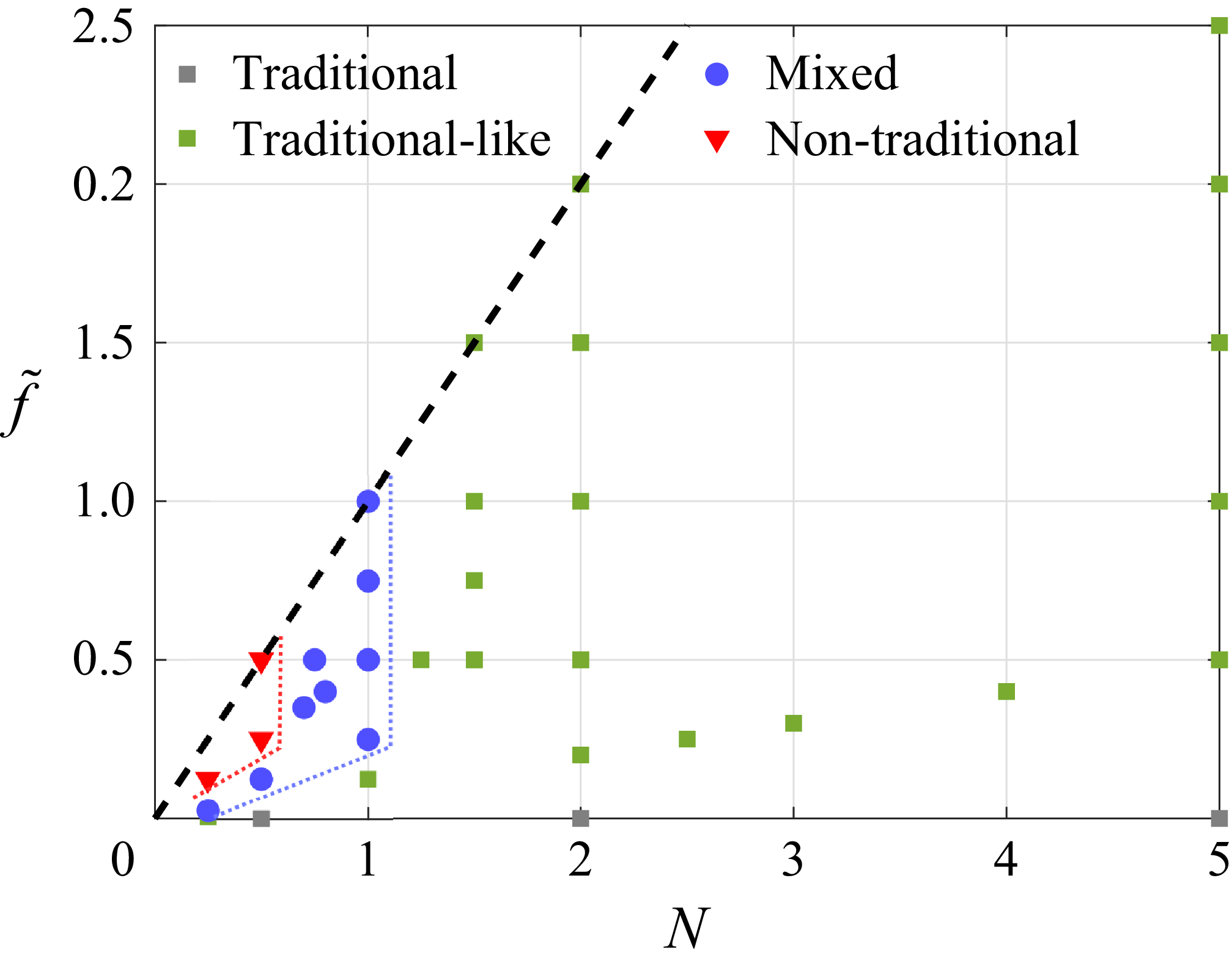Four distinct nonlinear evolutions have been observed as indicated by the different symbols in figure 3. The limits between the different domains are indicated approximately by red and blue dotted lines.

Figure 3.

Map of the simulations in the parameter space $(N,\tilde {f})$ for $ \textit{Re}=2000$ and $ \textit{Sc}=1$ . Grey, green, blue and red symbols represent the simulations where ‘traditional’, ‘traditional-like’, ‘mixed’ and ‘non-traditional’ behaviours have been observed, respectively. The black dashed line corresponds to the line $N=\tilde {f}$ delimiting the explored region in the present paper. The blue and red dotted lines indicate approximately the limits of the ‘mixed’ domain.

Figure 4.

Total vertical vorticity ( $\xi =\partial _x v-\partial _y u$ ) at (a) $t=60$ , (b) $t=67$ , (c) $t=78$ , (d) $t=200$ for $\tilde {f}=0$ , $ \textit{Re}=2000$ and $ \textit{Sc}=1$ (traditional evolution).

Figure 5.

Same as figure 4 but for $(N, \tilde {f})=(2, 1.5)$ and (a) $t=51$ , (b) $t=58$ , (c) $t=70$ , (d) $t=200$ (traditional-like evolution).The $y$ -axis has been cropped compared with the original computational domain.

Figure 6.

Same as figure 4 but for $(N, \tilde {f})=(1, 0.5)$ and (a) $t=65$ , (b) $t=73$ , (c) $t=145$ , (d) $t=200$ (mixed evolution).The $y$ -axis has been cropped compared with the original computational domain.

Figure 7.

Same as figure 4 but for $(N, \tilde {f})=(0.5, 0.5)$ and (a) $t=89$ , (b) $t=110$ , (c) $t=119$ , (d) $t=146$ (non-traditional evolution). The $y$ -axis has been cropped compared with the original computational domain.

First, the traditional evolution (figure 4) is observed for $\tilde {f}=0$ and any value of $N$ since the governing equations for the horizontal velocity ((2.5a ), (2.5b ), (2.5e )) are decoupled from those for $\hat {w}$ , $\hat {b}$ ((2.5c ), (2.5d )) when $\tilde {f}=0$ . As seen in figure 4, the total vertical vorticity $\xi =\partial _x v-\partial _y u$ evolves towards a quasisteady vortex. No pairing instability occurs since the streamwise length of the domain $L_{x}$ accommodates only one wavelength. As already mentioned, Appendix B describes the consequences of allowing two wavelengths to develop within a double-sized domain for the parameters $(N,\tilde {f})=(0.5, 0.5)$ .

When the stratification is sufficiently strong $N\gtrsim 1$ for any value of $\tilde {f}$ or when $N\lesssim 1$ for sufficiently low values of $\tilde {f}$ (green symbols in figure 3), the evolution of the total vertical vorticity (figure 5) is very similar to the one observed in the traditional limit. However, we can notice the generation of positive vorticity in the (reddish) region surrounding the vorticity braid. The negative vorticity also goes slightly below the initial minimum value $-1$ . This contrasts with the traditional case where the vertical vorticity is conserved in the inviscid limit and remains in the range $-1\leqslant \xi \leqslant 0$ for $ \textit{Re}=2000$ (figure 4). However, the instability generates a stable and coherent vortex like in figure 4. These cases will be called `traditional-like’ since we will see in the following that some differences exist compared with the traditional scenario depending on $N$ and $\tilde {f}$ .

For moderate stratification $0.7\lesssim N\lesssim 1$ and sufficiently large values of $\tilde {f}$ or for $N \lesssim 0.5$ and intermediates values of $\tilde {f}$ (blue symbols in figure 3), the total vertical vorticity first evolves like in the traditional case (figures 6 a and 6 b) but, subsequently, small secondary vortices develop within the core of the primary Kelvin–Helmholtz vortex (figures 6 c and 6 d). Nevertheless, it keeps its integrity. We can also notice that thin positive vorticity layers are generated and entrained inside or at the periphery of the Kelvin–Helmholtz vortex (figure 6 b,c,d). In addition, the minimum of the vertical vorticity decreases significantly below the initial value $-1$ . Such evolution will be termed as `mixed’ in the following.

Finally, when the stratification is weak $(N\leqslant 0.5)$ and $\tilde {f}$ larger than a critical value depending on $N$ ( $\tilde {f}\geqslant$ 0.25 for $N=0.5$ and $\tilde {f}\geqslant$ 0.125 for $N=0.25$ , red symbols in figure 3), the nonlinear evolution of the shear instability differs widely from the traditional case (figure 7). Thin layers with large positive and negative values of vertical vorticity are generated (figure 7 b) and, subsequently, stretched and amplified (figure 7 c) leading to an abrupt transition to small-scale turbulence (figure 7 d). This evolution will be called `non-traditional’ in the following. It is also noteworthy that the size in the $y$ direction of the developing Kelvin–Helmholtz billow is around 12, i.e. twice the one for the traditional case (figure 7 b compared with figure 4 c). This is the main reason why the size of the domain $L_{y}$ has to be increased for small and moderate values of $N$ as $\tilde {f}$ is increased (table 1). We can also notice that the shear instability appears slightly later (figure 7 a) since its growth rate is somewhat smaller than in the traditional limit (figure 2 a). Although this regime is represented by only three points in the parameter space (figure 3), several preliminary simulations with a lower resolution for other parameter values in this region are fully consistent with the existence of this regime.

The origin of these different behaviours of the vertical vorticity field is the vertical velocity and buoyancy. Indeed, while they are zero in the traditional limit, we see that the non-traditional Coriolis acceleration forces the vertical momentum (2.6c ) as soon as the streamwise velocity perturbation $\hat u$ is non-zero. Similarly, the advection of the base buoyancy $B$ by the cross-stream velocity $\hat v$ forces the buoyancy (2.6d ). In turn, the non-traditional Coriolis acceleration due to the vertical velocity forces the horizontal momentum (2.6a ). Equivalently, looking at the vertical vorticity equation,

(3.1) \begin{align} \frac {D \xi }{Dt}=\partial _{t}\hat {\xi }+U\partial _{x}\hat {\xi }-\hat {v}\partial _{y}^{2}U+\boldsymbol{\hat {u}}\boldsymbol{\cdot }\boldsymbol{\nabla }\hat {\xi }=\tilde {f}\partial _{y}\hat {w}+\frac {1}{\textit{Re}}{\nabla ^{2}}\hat {\xi }, \end{align}

where $D/Dt$ is the Lagrangian derivative and $\hat {\xi }=\partial _{x}\hat {v}-\partial _{y}\hat {u}$ is the vertical vorticity perturbation, we see that the right-hand side contains a tilting term of the horizontal background vorticity by the vertical velocity: $\tilde {f}\partial _{y}\hat {w}$ .

Figure 8 shows the vertical velocity at one instant for the traditional-like, mixed and non-traditional simulations. The instant displayed corresponds to the ones in figures 5(c), 6(b), 7(b), i.e. at the beginning of the nonlinear saturation regime and prior to the onset of secondary instabilities when they develop. In the three cases, the vertical velocity field has a global dipolar structure with positive/negative values on the left/right of the core of the primary vortex. Hence, the tilting term $\tilde {f}\partial _{y}\hat {w}$ of (3.1) is negative in the transverse band encompassing the vortex core and positive outside of it. This explains the appearance of vorticity in the regions surrounding the core and the braid (reddish and blueish regions in figures 5, 6, 7). In addition, thin bands of enhanced vertical velocity are superimposed on the dipolar structure of the vertical velocity, especially when $N \le 1$ . However, the main difference between the three cases is the amplitude of the vertical velocity: while its maximum is around 0.15 in figure 8(a), it is two and 10 times larger in figures 8(b) and 8(c), i.e. of the same order as the horizontal velocity. It is therefore not surprising that the vertical vorticity dynamics can be more or less modified compared with the traditional case due to the tilting term $\tilde {f} \partial _y \hat w$ on the right-hand side of (3.1).

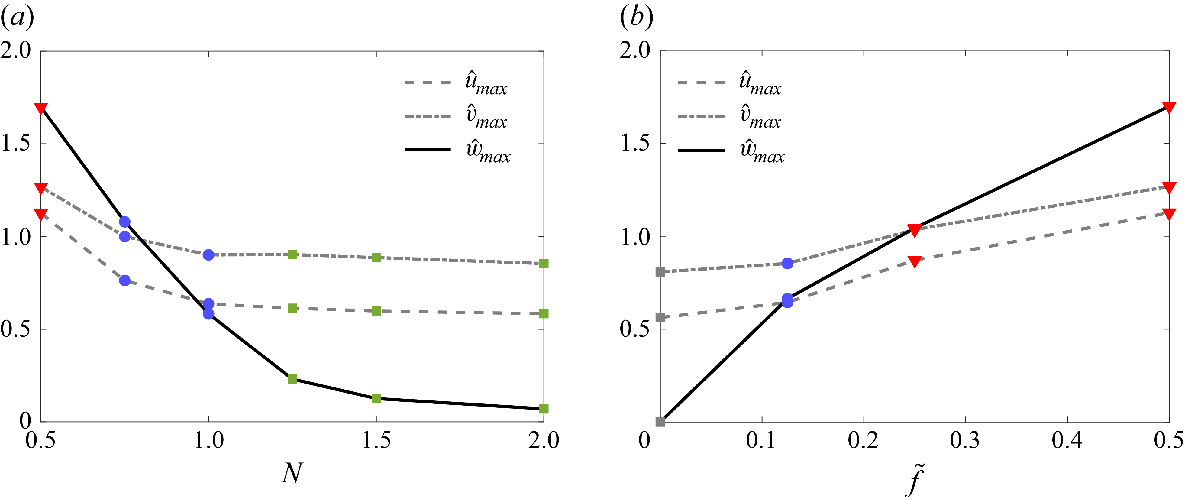
Figure 9 summarises the maxima of the three velocity components of the perturbation observed at the times prior to the onset of secondary instabilities (when they occur), for varying $N$ for $\tilde {f}=0.5$ (figure 9 a) and for varying $\tilde {f}$ for $N=0.5$ (figure 9 b). We see that the maximum of the vertical velocity increases when $N$ decreases for a fixed $\tilde {f}$ or when $\tilde {f}$ increases for a constant value of $N$ . In contrast, the maxima of the horizontal velocities ( $\hat {u}_{{max}}$ and $\hat {v}_{{max}}$ ) vary much less and remain always of order unity. The non-traditional and traditional-like evolutions are observed when the maximum vertical velocity is typically larger and much smaller than the maxima of the horizontal velocity components, respectively. The mixed evolution occurs when the maximum vertical velocity is in the intermediate range between these two cases.

Figure 8.

Vertical velocity for (a) $(N,\tilde {f})=(2,1.5)$ , $t=70$ , (b) $(N,\tilde {f})=(1,0.5)$ , $t=73$ , (c) $(N,\tilde {f})=(0.5,0.5)$ , $t=110$ for $ \textit{Re}=2000$ and $ \textit{Sc}=1$ .

Figure 9.

Maximum of the velocity component of the perturbation $\hat {w}$ (solid line), $\hat {u}$ (dashed line), $\hat {v}$ (dashed dotted line) observed at the beginning of the saturated regime and before the onset of secondary instabilities as a function of (a) $N$ for $\tilde {f}=0.5$ and (b) $\tilde {f}$ for $N=0.5$ . The symbols indicate the different nonlinear behaviours as in figure 3.

The approximate boundaries between the different domains in the parameter space depend both on $N$ and $\tilde {f}$ (red and blue dotted lines in figure 3). Although there are only few points in some regions, they seem, however, to occur for fixed values of the non-dimensional buoyancy frequency $N$ : $N \simeq 0.5$ and $N \simeq 1$ , for sufficiently large $\tilde {f}$ . This feature is reminiscent of the dynamics of a vertical vortex under the complete Coriolis acceleration in a stratified fluid (Toghraei & Billant Reference Toghraei and Billant2022). A strong vertical velocity field is generated when the buoyancy frequency is smaller than the maximum angular velocity of the vortex. This field develops near the critical radius where the angular velocity of the vortex is equal to the buoyancy frequency. In turn, the vertical velocity generates an anomaly of vertical vorticity which may trigger a shear instability above a critical non-traditional Coriolis parameter which depends on the Reynolds number.

In the present case, when the non-traditional parameter is weak, the vortex generated by the Kelvin–Helmholtz instability has a maximum absolute angular velocity approximately equal to 1/2 since the minimum vertical vorticity is around −1. Therefore, if the same mechanism as in Toghraei & Billant (Reference Toghraei and Billant2022) is at play, we could expect that strong vertical velocities may develop via critical layers when the non-dimensional Brunt–Väisälä frequency is less than $1/2$ . Since this critical value should probably be considered only as an order of magnitude, it could explain why the transition between the regimes in figure 3 seem to occur for fixed values of the non-dimensional buoyancy frequency $N$ . In addition, the thin bands of enhanced vertical velocity seen in figure 8 could be a signature of the presence of critical layers. However, it is difficult to make more quantitative comparisons since, here, the dynamics is more intricate and complicated than in Toghraei & Billant (Reference Toghraei and Billant2022). In particular, the Kelvin–Helmholtz vortex and the vertical velocity field develop concomitantly and there is an instantaneous mutual interaction between them, while the vortex is assumed to pre-exist in the study of Toghraei & Billant (Reference Toghraei and Billant2022).

3.2. Energy analysis

We now study the influence of the parameters $N$ and $\tilde {f}$ on the evolution of the kinetic and potential energies of the perturbations, defined as

(3.2) \begin{align} \hat {K}=\frac {1}{2L_{x}}\int _0^{L_x}\int _0^{L_y} \big(\hat {u}^2+\hat {v}^2+\hat {w}^2 \big){\rm d}y {\rm d}x, \quad \hat {P}=\frac {1}{2L_{x}}\frac {1}{N^2}\int _0^{L_x}\int _0^{L_y}\hat {b}^2\,{\rm d}y {\rm d}x, \end{align}

respectively. The surface integrals in (3.2) are normalised by $L_{x}$ , i.e. these energies are per unit wavelength in order to be able to compare simulations for different wavelengths. In contrast, they are not normalised by $L_y$ because the perturbations decay in the $y$ direction. In other words, the energies are $x$ -averaged and $y$ -integrated.

The kinetic energy can be further decomposed into horizontal and vertical components:

(3.3) \begin{align} \hat {K}_h=\frac {1}{2L_{x}}\int _0^{L_x}\int _0^{L_y} \big(\hat {u}^2+\hat {v}^2 \big){\rm d}y {\rm d}x, \quad \hat {K}_v=\frac {1}{2L_{x}}\int _0^{L_x}\int _0^{L_y}\hat {w}^2\,{\rm d}y {\rm d}x. \end{align}

Figure 10.

Evolutions of the (a,b) horizontal kinetic energy, (c,d) vertical kinetic energy and (e,f), potential energy of the perturbations for different stratifications $N$ and non-traditional parameter $\tilde {f}$ values for $ \textit{Re}=2000$ , $ \textit{Sc}=1$ : (a,c,e) $\tilde {f}=0.5$ and $N$ variable; (b,d,f) $N=2$ and $\tilde {f}$ variable.

Figure 10(a,c,e) shows the evolution of the horizontal and vertical kinetic energy and potential energy of the perturbations, for varying stratification $N$ and a non-traditional parameter fixed to $\tilde {f}=0.5$ . They all start at small values corresponding to the amplitude of the white noise and, after a transient period, increase exponentially before nonlinear saturation. However, the level of saturation oscillates slightly but regularly, especially when $N\geq 1$ . As discussed by Klaassen & Peltier (Reference Klaassen and Peltier1985a ) and Klaassen & Peltier (Reference Klaassen and Peltier1991), the oscillation is linked to a nutation of the Kelvin–Helmholtz vortex, during which an exchange of energy between the mean-flow and the perturbations occurs. The four typical nonlinear evolutions described in the previous section are present in figure 10(a,c,e), namely: traditional (figure 4), traditional-like for $N=2$ and $N=5$ (figure 5), mixed for $N=1$ and $N=0.75$ (figure 6) and non-traditional for $N=0.5$ (figure 7). As seen in figure 10(a), the level of saturation of the horizontal kinetic energy decreases as $N$ increases and tend, when $N\geqslant 1$ , to the traditional case (dashed line). When $N$ increases, the levels of saturation of the vertical kinetic energy and potential energy also decrease but in a much more pronounced manner than the horizontal kinetic energy. They are identically zero in the traditional limit (hence, not plotted), very low for $N=5$ while for $N=0.5$ , they are comparable to the horizontal kinetic energy. In § 3.5, we will further investigate what govern the levels of saturation of these different energies.

In turn, figure 10(b,d,f) show the evolution of the energies for a fixed stratification $N=2$ and varying $\tilde {f}$ . In this case, all the simulations shown exhibit a traditional-like behaviour. The growth rate and level of saturation of the horizontal kinetic energy slightly increases with $\tilde {f}$ but remains close to the one in the traditional limit (figure 10 b). In contrast, the amplitudes of saturation of the vertical kinetic energy and potential energy (figure 10 d,f) increase strongly with $\tilde {f}$ but they remain below the level of the horizontal kinetic energy for $\tilde {f}\leqslant N$ . Analytical expressions for the energies in terms of $N$ and $\tilde {f}$ will be derived in § 3.5 in the limit of strong stratification. In summary, the stratification and non-traditional effects have a competing influence on the nonlinear dynamics of the shear instability: when the stratification is increased keeping $\tilde {f}$ constant, the evolutions of the energies tend to the traditional ones while, when the non-traditional parameter is increased for fixed $N$ , they depart more and more from the traditional case.

3.3. Enstrophy analysis

The evolution of the total enstrophy,

(3.4) \begin{align} Z=\frac {1}{2L_{x}}\int _0^{L_x}\int _0^{L_y}\boldsymbol{\omega }^{2}\,{\rm d}y {\rm d}x, \end{align}

where $\boldsymbol{\omega }$ is the total vorticity $\boldsymbol{\omega }=\boldsymbol{\omega _{h}}+\xi \boldsymbol{e_{z}}$ , with $\boldsymbol{\omega _{h}}=\partial _{y}w\boldsymbol{e_{x}}-\partial _{x}w\boldsymbol{e_{y}}$ the horizontal vorticity, has been studied for the four simulations presented in § 3.1. Like for the energy, the total enstrophy can be further decomposed into horizontal and vertical components,

(3.5) \begin{align} Z_{h}=\frac {1}{2L_{x}}\int _0^{L_x}\int _0^{L_y}\omega _{h}^{2}\,{\rm d}y {\rm d}x, \quad Z_{v}=\frac {1}{2L_{x}}\int _0^{L_x}\int _0^{L_y}\xi ^{2}\,{\rm d}y {\rm d}x. \end{align}

Equivalent quantities denoted with a hat $\hat {Z}$ , $\hat {Z}_{h}$ , $\hat {Z}_{v}$ can be defined for the vorticity of the perturbation $\boldsymbol{\hat {\omega }}$ .

Figure 11.

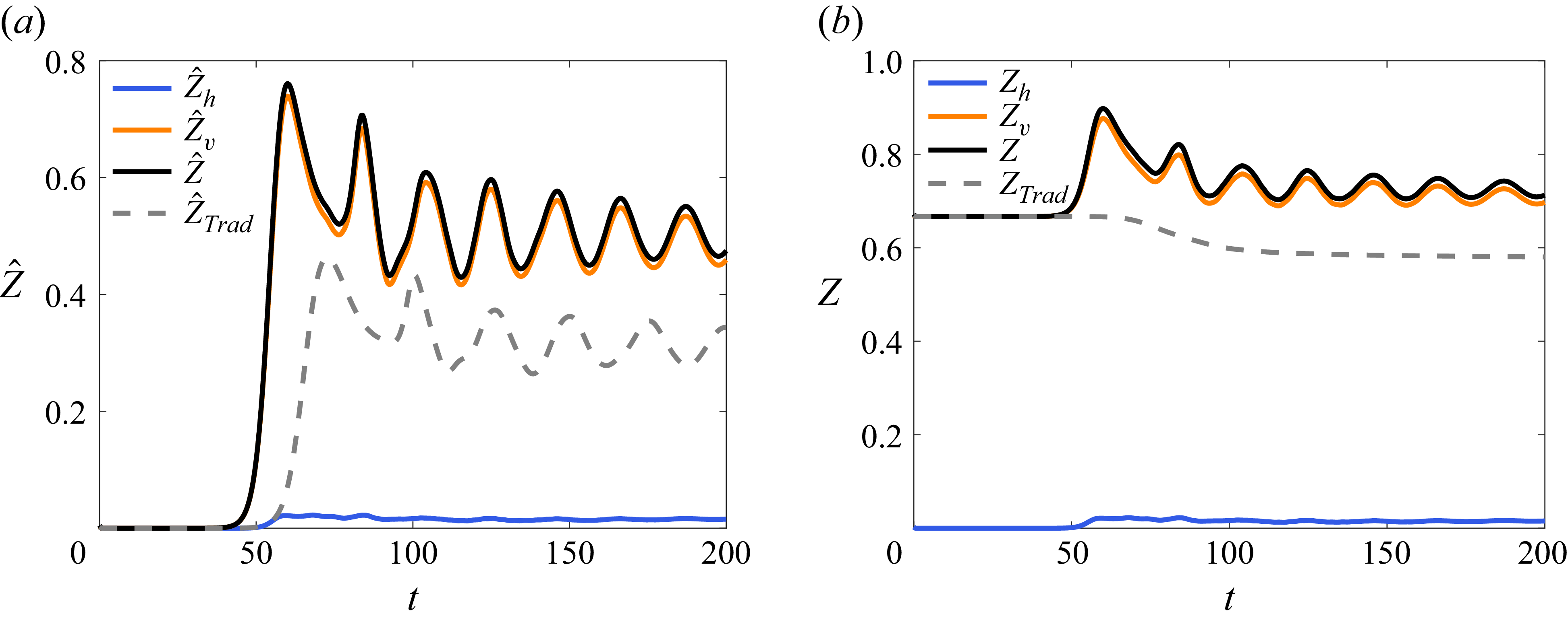
(a) Evolution of the horizontal (blue line), vertical (orange line) and total (black line) enstrophy of the perturbations for $(N, \tilde {f})=(2, 1.5)$ . The grey dashed line corresponds to the total enstrophy of the perturbation in the traditional limit. Panel (b) is the same as (a) but for the total enstrophies $Z_{h}$ , $Z_{v}$ and $Z$ .

Figure 12.

(a) Evolution of the horizontal (blue line), vertical (orange line) and total (black line) enstrophy of the perturbations for $(N, \tilde {f})=(1, 0.5)$ . Panel (b) is the same as (a) but for the total enstrophies $Z_{h}$ , $Z_{v}$ and $Z$ .

Figure 11 shows the evolutions of $\hat {Z}_{h}$ , $\hat {Z}_{v}$ , $\hat {Z}$ and of the total enstrophy for the simulation in the traditional limit (figure 4) and for the traditional-like simulation for $(N, \tilde {f})=(2, 1.5)$ (figure 5). In the traditional limit, only the total enstrophy is shown (dashed line) since the horizontal enstrophy remains zero. As seen in figure 11(a), the enstrophy of the perturbations for $\tilde {f}=0$ rises exponentially and then tends to saturate but with some oscillations superimposed as observed for the kinetic energy. The total enstrophy $Z$ (dashed line in figure 11 b) decreases monotonically as expected since the flow is purely two-dimensional for $\tilde {f}=0$ . The total decay of $Z$ is, however, relatively small (note the vertical scale). We remind that the dissipation of the base flow is not taken into account.

For the traditional-like simulation (solid lines in figure 11), the horizontal enstrophy remains always small since the vertical velocity is small. The evolution of $\hat {Z}$ is very similar to the one in the traditional limit but with a higher value as the maximum and minimum vertical vorticity are no longer 0 and −1 but are outside this range. For this reason, the total enstrophy $Z$ increases somewhat before oscillating (figure 11 b). This is possible since the vorticity is no longer conserved in the inviscid limit for non-zero $\tilde {f}$ .

Figure 12 shows the evolution of the enstrophy for the mixed case for $(N, \tilde {f})=(1, 0.5)$ (figure 6). The vertical enstrophy of the perturbation $\hat {Z}_{v}$ saturates at approximately the same level as in figure 11. When $\hat {Z}_{v}$ begins to saturate, the horizontal enstrophy of the perturbation $\hat {Z}_{h}$ starts to grow and becomes dominant afterwards. Thereby, the total enstrophy (figure 12 b) increases significantly instead of decaying. The total vertical enstrophy remains approximately constant. It is worth pointing out that the increase of the enstrophies of the perturbation occurs during the linear and nonlinear stages of the primary Kelvin–Helmholtz instability while the secondary instabilities develop only later $t\geqslant 120$ (small wiggles are then visible on the curves in figure 12).

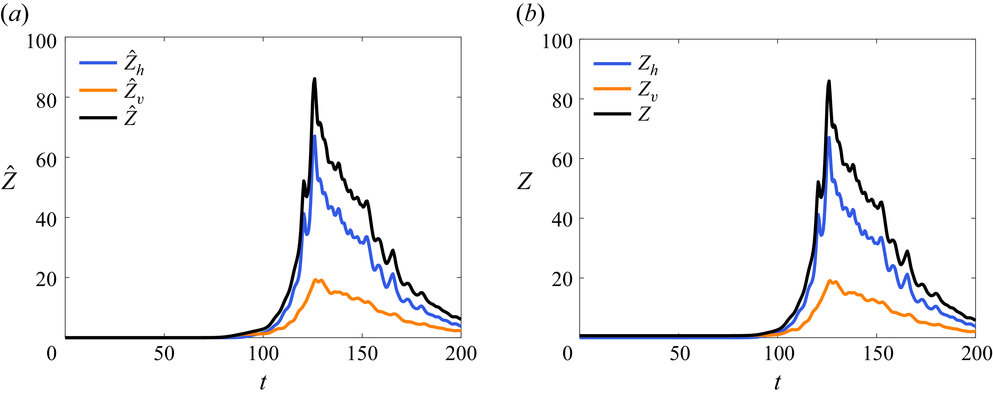
For the non-traditional case for $(N, \tilde {f})=(0.5, 0.5)$ (figure 13), there is a dramatic increase of the horizontal enstrophy of the perturbation up to $\hat {Z}_{h}\sim 70$ and then it eventually decays. The vertical enstrophy $\hat {Z}_{v}$ increases also but in a less pronounced manner. It is interesting to note that both components of enstrophy begin to increase when the nonlinear regime sets in at $t\sim 90$ as in figure 12, but the main increase actually occurs later at $t\sim 120$ when the secondary instabilities develop and the flow becomes turbulent. A high peak of enstrophy has been also observed by Staquet (Reference Staquet1995) when secondary instabilities develop in a stratified vertically sheared flow. The influence of the Reynolds number and Schmidt number on the level of this enstrophy maximum will be investigated in a future paper.

Figure 13.

Same as figure 12 but for $(N, \tilde {f})=(0.5, 0.5)$ .

To interpret the evolution of the enstrophy, we consider the equation for the vertical vorticity (3.1) and the one for the horizontal vorticity of the perturbations $\boldsymbol{\hat {\omega }_{h}}$ , which can be derived from (2.6):

(3.6) \begin{align} \displaystyle \partial _t \boldsymbol{\hat {\omega }_{h}}+U\partial _x\boldsymbol{\hat {\omega }_{h}}+(\boldsymbol{\hat {u}}\boldsymbol{\cdot }\boldsymbol{\nabla })\boldsymbol{\hat {\omega }_{h}}=\tilde {f}\partial _{y}\boldsymbol{\hat {u}}+(\boldsymbol{\hat {\omega }_{h}}\boldsymbol{\cdot }\boldsymbol{\nabla })(U\boldsymbol{e_{x}}+\boldsymbol{\hat {u}})+\boldsymbol{\nabla }\times (\hat {b}\boldsymbol{e_{z}})+\frac {1}{\textit{Re}}{\nabla ^2}\boldsymbol{\hat {\omega }_{h}}. \end{align}

It is worth noticing that the right-hand side of (3.6) contains the following effects: first, the tilting and stretching of the horizontal background vorticity $\tilde {f}$ ; second, the tilting and stretching of the horizontal vorticity of the perturbation by the base flow and the velocity of the perturbations; third, the baroclinic torque and, finally, the viscous effects.

Equations (3.1) and (3.6) can be combined to give an equation for the evolution of the enstrophy of the perturbation,

(3.7a) \begin{align} \displaystyle \frac {D\hat {Z}}{Dt}&=\mathcal{S}+\mathcal{I}+\mathcal{B}+\mathcal{D},\,\,\,\,\quad\quad\quad\quad\quad\quad\quad\quad\quad\quad\quad\quad\quad\quad\quad\quad\quad\quad\quad\quad \\[-9pt] \nonumber \end{align}

where

(3.7b) \begin{align} \displaystyle \mathcal{S}&=\frac {1}{L_{x}}\int _{0}^{L_{x}}\int _{0}^{L_{y}}\boldsymbol{\hat {\omega }}\boldsymbol{\cdot }\left [(\boldsymbol{\hat {\omega }}+\tilde {f}\boldsymbol{e_{y}})\boldsymbol{\cdot }\boldsymbol{\nabla }\boldsymbol{\hat {u}}\right ]\,{\rm d}y{\rm d}x, \\[-9pt] \nonumber \end{align}

(3.7c) \begin{align} \displaystyle \mathcal{I}&=\frac {1}{L_{x}}\int _{0}^{L_{x}}\int _{0}^{L_{y}}\boldsymbol{\hat {\omega }}\boldsymbol{\cdot }\left [(\boldsymbol{\hat {\omega }}\boldsymbol{\cdot }\boldsymbol{\nabla })U\boldsymbol{e_{x}}+(\boldsymbol{\omega _{b}}\boldsymbol{\cdot }\boldsymbol{\nabla })\boldsymbol{\hat {u}}-(\boldsymbol{\hat {u}}\boldsymbol{\cdot }\boldsymbol{\nabla })\boldsymbol{\omega _{b}}\right ]\,{\rm d}y{\rm d}x, \\[-9pt] \nonumber \end{align}

(3.7d) \begin{align} \displaystyle \mathcal{B}&=\frac {1}{L_{x}}\int _{0}^{L_{x}}\int _{0}^{L_{y}}\boldsymbol{\hat {\omega }}\boldsymbol{\cdot }\boldsymbol{\nabla }\times (\hat {b}\boldsymbol{e_{z}})\,{\rm d}y{\rm d}x, \\[-9pt] \nonumber \end{align}

(3.7e) \begin{align} \displaystyle \mathcal{D}&=-\frac {1}{L_{x}}\frac {1}{\textit{Re}}\int _{0}^{L_{x}}\int _{0}^{L_{y}}(\boldsymbol{\nabla }\boldsymbol{\hat {\omega }})^{2}\,{\rm d}y{\rm d}x, \\[9pt] \nonumber \end{align}

are, respectively, stretching/tilting effect, interaction with the base flow, baroclinic and viscous effects. Here $\boldsymbol{\omega _{b}}=-\partial _{y}U\,\boldsymbol{e_{z}}$ is the vorticity of the base flow.

Figure 14.

Different terms of the enstrophy budget (3.7) for (a) $(N, \tilde {f})=(5, 0)$ , (b) $(N, \tilde {f})=(2, 1.5)$ , (c) $(N, \tilde {f})=(1, 0.5)$ , (d) $(N, \tilde {f})=(0.5, 0.5)$ .

Figure 14(a) shows these four terms in the traditional case. Only the interaction with the base flow and the dissipation contribute to the enstrophy budget as expected. In the traditional-like case for $(N, \tilde {f})=(2, 1.5)$ , a similar evolution is observed (figure 14 b) except that the baroclinic term is of the same order as the interaction with the base flow. The stretching/tilting term is no longer exactly zero but remains small. For the mixed case for $(N, \tilde {f})=(1, 0.5)$ (figure 14 c), the interaction, baroclinic and dissipation terms are still dominant but the stretching/tilting is almost of the same order. It can be noticed also that the dissipation term is one order of magnitude larger than in the previous cases. Finally, for the non-traditional case for $(N, \tilde {f})=(0.5, 0.5)$ , figure 14(d) shows that the considerable increase of $\hat {Z}$ (figure 13 a) is due to the vortex stretching/tilting that becomes, by far, the dominant source of enstrophy when secondary instabilities develop at $t\geqslant 120$ . Simultaneously, the dissipation (in absolute value) grows to the same level: it is the dissipative anomaly linked to the development of turbulence. These pronounced peaks are indeed observed when secondary instabilities arise and lead to a transition to turbulence. Such enstrophy evolution is characteristic of a three-dimensional flow even if the present configuration is only two-dimensional. This is because the flow has three velocity components, enabling the stretching and tilting of vorticity. In contrast, the interaction with the base flow and the baroclinic terms are much smaller.

3.4. Origin of secondary instabilities

In this section, we analyse the origin of secondary instabilities observed in the `mixed’ simulation for $(N,\tilde {f})=(1, 0.5)$ and in the `non-traditional’ simulation for $(N,\tilde {f})=(0.5, 0.5)$ (see figure 3). In the first case, the secondary instabilities develop in the periphery of the vortex core but remain localised (figures 6 c and 6 d). In the second case $(N,\tilde {f})=(0.5, 0.5)$ , the secondary instabilities arise in the same region but quickly contaminate the whole flow and lead to a transition to small-scale turbulence (figure 7 c,d).

In order to interpret the origin of these instabilities, we will check whether or not the Fjørtoft necessary condition for instability is satisfied (Fjørtoft Reference Fjørtoft1950). It is a more stringent criterion than the inflection point condition of Rayleigh. For an inviscid parallel shear flow, it reads

(3.8) \begin{align} \partial _{yy}u(y)(u(y)-u(y_{i}))\lt 0, \end{align}

where $u(y_{i})$ is the velocity at the inflection point $y_{i}$ . There exists also a version of this criterion for an inviscid axisymmetric vortex (Fjørtoft Reference Fjørtoft1950; Smyth & Carpenter Reference Smyth and Carpenter2019),

(3.9) \begin{align} \partial _{r}\xi (r)(\varOmega (r)-\varOmega (r_{i}))\lt 0, \end{align}

where $(r, \theta , z)$ are cylindrical coordinates in the radial, azimuthal and vertical directions, respectively. Here $\xi$ is the axial vorticity, $\varOmega$ the angular velocity and $r_{i}$ the inflection point where $\partial _{r}\xi (r_{i})=0$ .

As shown by Smyth & Carpenter (Reference Smyth and Carpenter2019), the Fjørtoft criterion in Cartesian coordinates is equivalent to require that the inflection point is a maximum of shear:

(3.10) \begin{align} S=\sqrt {(\partial _{y}u)^{2}+(\partial _{x}v)^{2}}. \end{align}

Although these criteria are strictly valid for an axisymmetric vortex and for a parallel shear flow, we will apply them to the flows observed prior to the secondary instabilities onset in the ‘mixed case’ and in the ‘non-traditional’ case, respectively. Indeed, as seen in figure 15(a), the vortex in the mixed case is approximately axisymmetric whereas, in the non-traditional case (figure 15 b), the vorticity filaments are strongly elongated and can be reasonably approximated as locally parallel. Furthermore, one can remark that these criteria apply only to traditional flows, i.e. purely two-dimensional flows, which is not the case here. Nonetheless, the typical scale $\ell$ of the vorticity filaments is much smaller than the initial scale $L_{0}$ of the shear flow: $\ell \ll L_{0}$ . This implies that the local non-dimensional Brunt–Väisälä frequency $N_{\ell }$ and non-traditional Coriolis parameter $\tilde {f}_{\ell }$ are much smaller: $N_{\ell }=N_{0}\ell /U_{0}=N\ell /L_{0}\ll 1$ and $\tilde {f}_{\ell }=\tilde {f}_{0}\ell /U_{0}=\tilde {f}\ell /L_{0}\ll 1$ . Thus, we have $N_{\ell }\simeq 0$ and $\tilde {f}_{\ell }\simeq 0$ and it is legitimate to assume that the local dynamics is approximately two-dimensional.

Figure 15.

Total vertical vorticity $\xi$ at (a) $t=112$ for $(N,\tilde {f})=(1, 0.5)$ and at (b) $t=117.5$ for $(N,\tilde {f})=(0.5, 0.5)$ . The black solid lines indicate the lines along which Fjørtoft criteria are computed. (c,d) Shear $S$ corresponding to (a) and (b). (e) Vorticity (blue) and cylindrical Fjørtoft criterion (3.9) (orange), computed along the black line in (a). The centre of the vortex corresponds to $r=0$ . (f) Vorticity (blue) and cartesian Fjørtoft criterion (3.8) (orange) along the black line in (b). The black dotted vertical lines in (e) and (f) indicate the location of $r_i$ and $y_i$ , respectively.

In the mixed case $(N,\tilde {f})=(1, 0.5)$ , figure 15(c) shows that $S$ is maximum in the region where secondary instabilities will develop a few time units later. In addition, the criterion (3.9) is computed along the solid black line in figure 15(a) and the results are presented in figure 15(e). It is indeed satisfied around the inflection point which is at $r=1.96$ . Furthermore, the associated vorticity profile exhibits also a minimum at $r=2.2$ , i.e. there is a second inflection point. Therefore, the configuration is similar to that of a jet, with contiguous maximum and minimum of vorticity. The instability (figure 6 c) indeed resembles the most unstable mode of jet instability, i.e. the sinuous mode.

For the non-traditional case $(N,\tilde {f})=(0.5, 0.5)$ , the maximum of shear (figure 15 d) is also located in the region where the secondary instabilities will emerge, but it is much more intense than in the previous case. Figure 15(f) shows the cartesian Fjørtoft criterion (3.8) along the straight black line drawn in figure 15(b) across the corresponding vorticity filament. In this case, there is a single inflection point located at $y_{i}=34.52$ (figure 15 f) like for a shear layer. The cartesian Fjørtoft criterion for instability (3.8) is satisfied in its neighbourhood.

Therefore, in both mixed and non-traditional simulations, the secondary instabilities can be interpreted as new shear instabilities developing on the vertical vorticity anomalies generated by non-traditional effects.

3.5. Analysis for strong stratification

In this section, we will show that the governing equation (2.6) can be greatly simplified when the stratification is strong. This will enable us to derive scaling laws for the kinetic and potential energies in terms of $N$ and $\tilde {f}$ when $N\gg 1$ . We will consider the inviscid limit for simplicity but the following analysis is expected to be valid as long as the Reynolds number is large.

By taking the derivative $D/Dt=\partial _{t}+U\partial _{x}+\boldsymbol{\hat {u}}\boldsymbol{\cdot }\boldsymbol{\nabla }$ of (2.6c ), by using (2.6d ) and (2.6a ), the buoyancy can be eliminated, giving

(3.11) \begin{align} \frac {D^2\hat {w}}{Dt^2}+ \big(\tilde {f}^2+N^2 \big)\hat {w}=-\tilde {f}\partial _x\hat {p}. \end{align}

Even if the linear stability analysis shows that the maximum growth rate $\sigma _{{m}}$ and most amplified wavenumber $k_{x{m}}$ vary somewhat with $N$ and $\tilde {f}$ , we will assume a priori here that $D/Dt\sim O(\sigma _{{m}})\sim O(k_{x{m}})\sim O(1)$ . Therefore, when $N^{2}+\tilde {f}^{2}\gg 1$ , (3.11) simplifies to

(3.12) \begin{align} \hat {w}\simeq \frac {-1}{\tilde {f}\left (1+\left (\frac {N}{\tilde {f}}\right )^2\right )}\partial _x\hat {p}. \end{align}

The approximation (3.12) seems to be valid as soon as $N^{2}+\tilde {f}^{2}\gg 1$ , i.e. if either $N\gg 1$ or/and $\tilde {f}\gg 1$ . However, we will see a posteriori that the final results are self-consistent with the approximation (3.12) only if $N\gg 1$ .

Inserting (3.12) in the horizontal momentum ((2.6a ), (2.6b ) and (2.6e ) leads to a closed system of equations for $(\hat {u}, \hat {v}, \hat {p})$ ,

(3.13a) \begin{align} \displaystyle \partial _t \hat {u}+U\partial _x\hat {u}+\hat {v}\partial _y U+\hat {u}\partial _{x}\hat {u}+\hat {v}\partial _{y}\hat {u}&=-\alpha \partial _x \hat {p}, \\[-9pt] \nonumber \end{align}

(3.13b) \begin{align} \displaystyle \partial _t \hat {v}+U\partial _x\hat {v}+\hat {u}\partial _{x}\hat {v}+\hat {v}\partial _{y}\hat {v}&=-\partial _y \hat {p}, \\[-9pt] \nonumber \end{align}

(3.13c) \begin{align} \partial _x \hat {u}+\partial _y \hat {v}&=0, \\[9pt] \nonumber \end{align}

which are very similar to the equations in the traditional limit except for the presence of the parameter $\alpha$ in (3.13a ):

(3.14) \begin{align} \alpha =\frac {N^{2}}{\tilde {f}^{2}+N^{2}}. \end{align}

This parameter is a measure of the non-traditional Coriolis parameter compared with the Brunt–Väisälä frequency: it is equal to unity in the traditional limit $\tilde {f}=0$ , and it decreases as $\tilde {f}/N$ increases. When $\tilde {f}$ is non-zero, (3.13) can be, however, transformed into the traditional equations by applying the following change of variables:

(3.15) \begin{align} \hat {u}=\hat {u}', \quad \hat {v}=\frac {1}{\sqrt {\alpha }}\hat {v}', \quad \hat {p}=\frac {1}{\alpha }\hat {p}', \\[-28pt] \nonumber \end{align}

(3.16) \begin{align} \partial _{x}=\frac {1}{\sqrt {\alpha }}\partial _{x}', \quad \partial _{y}=\partial _{y}', \quad \partial _{t}=\frac {1}{\sqrt {\alpha }}\partial _{t}'. \\[-2pt] \nonumber \end{align}

Indeed, the equations for the primed variables are strictly two-dimensional:

(3.17a) \begin{align} \displaystyle \partial _t' \hat {u}'+U\partial _x'\hat {u}'+\hat {v}'\partial _y' U+\hat {u}'\partial _{x}'\hat {u}'+\hat {v}'\partial _{y}'\hat {u}'&=-\partial _x' \hat {p}', \\[-9pt] \nonumber \end{align}

(3.17b) \begin{align} \displaystyle \partial _t' \hat {v}'+U\partial _x'\hat {v}'+\hat {u}'\partial _{x}'\hat {v}'+\hat {v}'\partial _{y}'\hat {v}'&=-\partial _y' \hat {p}', \\[-9pt] \nonumber \end{align}

(3.17c) \begin{align} \partial _x'\hat {u}'+\partial _y'\hat {v}'&=0. \\[9pt] \nonumber \end{align}

Before discussing some properties associated with (3.17) and (3.15)–(3.16), we first check a posteriori whether or not the assumption $N^{2}+\tilde {f}^{2}\gg d^{2}/{\rm d}t^{2}$ used to derive (3.17) is satisfied. The change of variable (3.16) implies that $D/Dt\sim \partial _{t}\sim \partial _{x}=O(1/\sqrt {\alpha })$ since $\partial _{t}'\sim O(1)$ and $\partial _{x}'\sim O(1)$ . Hence, we should have

(3.18) \begin{align} N^{2}+\tilde {f}^{2}\gg 1/\alpha . \end{align}

From (3.14), we see that this is the case only if $N^{2}\gg 1$ and not if $\tilde {f}\gg 1$ with $N\leqslant O(1)$ contrary to what (3.11) suggests. Hence, the reduced system (3.13) is expected to be valid only if the stratification is strong, i.e. $N\gg 1$ .

The transformation (3.15)–(3.16) has several interesting properties. First, concerning the linear stability of the base flow (§ 2.3), it implies that the dispersion relation for any $\tilde {f}$ and $N\gg 1$ is $\sigma =\mathcal{F}(k_{x}\sqrt {\alpha })/\sqrt {\alpha }$ , where $\sigma =\mathcal{F}(k_{x})$ is the dispersion relation for $\tilde {f}=0$ . Figure 2(b) indeed shows that the rescaled growth rate $\sigma \sqrt {\alpha }$ represented as a function of $k_{x}\sqrt {\alpha }$ collapses towards the growth rate curve for $\tilde {f}=0$ when $N\gg 1$ and $\tilde {f}$ is non-zero.

Another important property of (3.17) is that the total vertical vorticity $\xi '=\partial _{x}'\hat {v}'-\partial _{y}'\hat {u}'-\partial _{y}'U$ is conserved following the motion since these equations are purely two-dimensional. When rewritten in terms of the unprimed variables, the total vertical vorticity becomes $\xi '=\alpha \partial _{x}\hat {v}-\partial _{y}\hat {u}-\partial _{y}U$ and its governing equation remains

(3.19) \begin{align} \partial _{t}\xi '+U\partial _{x}\xi '+\boldsymbol{\hat {u}}\boldsymbol{\cdot }\boldsymbol{\nabla }\xi '=0. \end{align}

It can be easily shown that (3.19) derives from the conservation of potential vorticity $\varPi =(\boldsymbol{\omega }+\tilde {f}\boldsymbol{e_{y}})\boldsymbol{\cdot }(N^{2}\boldsymbol{e_{z}}+\boldsymbol{\nabla }b)$ .

In the following sections, we further show that the levels of saturation of the different energy components for any $\tilde {f}$ and sufficiently large $N$ can be deduced from those for $\tilde {f}=0$ thanks to the transformation (3.15)–(3.16).

3.5.1. Scaling for the horizontal kinetic energy of the perturbation

The transformation (3.15)–(3.16) implies that the horizontal kinetic energy can be written as

(3.20) \begin{align} \hat {K}_h=\frac {1}{2L_{x}}\int _0^{L_x}\int _0^{L_y} \big(\hat {u}^2+\hat {v}^{2} \big)\,{\rm d}y {\rm d}x=\frac {1}{2L_{x}'}\int _0^{L_x'}\int _0^{L_y'}\left (\hat {u}'^2+\frac {\hat {v}'^2}{\alpha }\right )\,{\rm d}y' {\rm d}x', \end{align}

where $L_{x}'=L_{x}\sqrt {\alpha }$ and $L_{y}'=L_{y}$ .

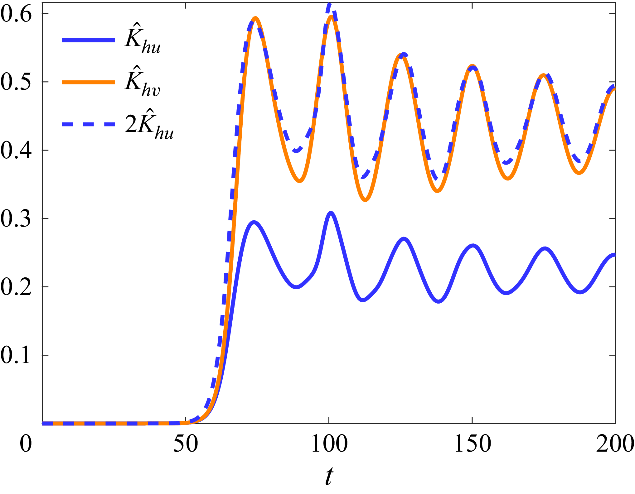
The numerical simulations show that, at saturation, we have the empiric approximate relation (see figure 16),

(3.21) \begin{align} \int _0^{L_x'}\int _0^{L_y'}\hat {v}'^2\,{\rm d}y' {\rm d}x' \simeq 2 \int _0^{L_x'}\int _0^{L_y'}\hat {u}'^2\,{\rm d}y' {\rm d}x' . \end{align}

Figure 16.

Evolution of $\displaystyle \hat {K}_{hu}= 1/(2L_x)\int _0^{L_x}\int _0^{L_y}\hat {u}^2\,{\rm d}y {\rm d}x$ and $\displaystyle \hat {K}_{hv}= 1/(2L_x)\int _0^{L_x}\int _0^{L_y}\hat {v}^2\,{\rm d}y {\rm d}x$ for $\tilde {f}=0$ , $ \textit{Re}=2000$ and $ \textit{Sc}=1$ . The dashed line, which represents $2\hat {K}_{hu}$ shows that $\hat {K}_{hv}\simeq 2\hat {K}_{hu}$ as assumed in (3.21).

Therefore, the horizontal kinetic energy for any $\tilde {f}$ and $N\gg 1$ is approximately given by

(3.22) \begin{align} \hat {K}_h\simeq \frac {1}{3}\left (3+2\left (\frac {\tilde {f}}{N}\right )^{2}\right )\hat {K}_h', \end{align}

where $\hat {K}_h'$ is the horizontal kinetic energy for $\tilde {f}=0$ . Thus, the horizontal kinetic energy of the perturbations depends only on the ratio $\tilde {f}/N$ . It increases with $\tilde {f}$ and decreases with $N$ in agreement with the trends observed in figure 10. The relation (3.22) is further tested in figure 17. Figure 17(a) displays the evolutions of $\hat {K}_h$ for various sets of parameters $(N, \tilde {f})$ such that $N\geqslant 1$ . Figure 17(b) shows $\hat {K}_h$ rescaled by $(1+2/3(\tilde {f}/N)^{2})$ for the same parameters. All the horizontal kinetic energies in the saturated regime then collapse approximately around the same mean value. This value is indicated in figure 17(b) by a horizontal black dotted line corresponding to the mean horizontal kinetic energy at saturation of the simulation for $(N,\tilde {f})=(5, 0.5)$ which is closest to the traditional limit. We can notice that even the curve for $(N, \tilde {f})=(1, 1)$ collapses relatively well on the others, even if $N$ is not much larger than unity.

Figure 17.

(a) Horizontal kinetic energy of the perturbations for different parameters $N$ and $\tilde {f}$ . (b) Horizontal kinetic energy of the perturbations rescaled by $A=(1+(2/3)(\tilde {f}/N)^{2})$ for the same parameters as in (a). The black dotted line in (b) shows the mean value towards which the rescaled curves collapse.

3.5.2. Scaling for the vertical kinetic energy

Using (3.12) and the transformation (3.15)–(3.16), the vertical velocity can be written as

(3.23) \begin{align} \hat {w}\simeq -\frac {\tilde {f}}{N^{2}+\tilde {f}^{2}}\frac {\partial _{x}'\hat {p}'}{\alpha ^{3/2}}. \end{align}

Hence, the vertical kinetic energy can be expressed as

(3.24) \begin{align} \hat {K}_v=\frac {1}{2L_{x}}\int _0^{L_x}\int _0^{L_y}\hat {w}^2\,{\rm d}y {\rm d}x\simeq \left (\frac {\tilde {f}}{N}\right )^{2}\left (\frac {N^{2}+\tilde {f}^{2}}{N^{4}}\right )\left (\frac {1}{2L_{x}'}\int _0^{L_x'}\int _0^{L_y'} \big(\partial _{x}'\hat {p}' \big)^2\,{\rm d}y' {\rm d}x' \! \right )\!. \end{align}

Figure 18.

(a) Vertical kinetic energy of the perturbations for different parameters $N$ and $\tilde {f}$ . (b) Vertical kinetic energy of the perturbations rescaled by $ A = (\tilde {f}/N)^{2}(\tilde {f}^{2}+N^{2})/N^{4}$ for the same parameters as in (a). The black dotted line in (b) shows the mean value towards which the rescaled curves collapse.

In other words, $\hat {K}_v$ should be proportional to the factor $A=(\tilde {f}/N)^{2}(1+(\tilde {f}/N)^{2})/N^{2}$ . As seen in figure 18(a), the vertical kinetic energy saturates at very different levels when $\tilde {f}$ and $N$ are varied (keeping $N\geqslant 1$ ) but when rescaled by $A$ (figure 18 b), all the curves collapse around the same mean level of saturation (shown by a black dotted line). The rescaled vertical kinetic energy for $(N, \tilde {f})=(1, 1)$ is 30 % away from the others since the assumption $N\gg 1$ is less well verified than for the other sets of parameters.

3.5.3. Scaling for the potential energy

Similarly, the vertical momentum (2.6c ) in the inviscid limit, i.e.

(3.25) \begin{align} \frac {D\hat {w}}{Dt}-\tilde {f}\hat {u}=\hat {b} \end{align}

can be used to obtain an expression for $\hat {b}$ in terms of primed quantities, thanks to (3.15), (3.16) and (3.23):

(3.26) \begin{align} \hat {b}=-\tilde {f}\hat {u}'+\left (\frac {\tilde {f}}{N}\right )^{2}\left (1+\left (\frac {\tilde {f}}{N}\right )^{2}\right )\frac {D}{Dt'} \big(\partial _{x}'\hat {p}' \big). \end{align}

It shows that for strong stratification $N\gg 1$ , the buoyancy can be approximated by $\hat {b}=-\tilde {f}\hat {u}'$ , which corresponds to the quasihydrostatic balance, i.e. the hydrostatic equilibrium in presence of the non-traditional Coriolis force (Gerkema et al. Reference Gerkema, Zimmerman, Maas and van Haren2008) and in the absence of the vertical pressure gradient.

Therefore, the potential energy of the perturbations can be approximated by

(3.27) \begin{align} \hat {P}=\frac {1}{2L_{x}N^{2}}\int _0^{L_x}\int _0^{L_y}\hat {b}^2\,{\rm d}y {\rm d}x\simeq \left (\frac {\tilde {f}}{N}\right )^{2}\frac {1}{2L_{x}'}\int _0^{L_x'}\int _0^{L_y'}\hat {u}'^{2}\,{\rm d}y' {\rm d}x'. \end{align}

Figure 19.

(a) Potential energy of the perturbations for different parameters $N$ and $\tilde {f}$ . (b) Potential energy of the perturbations rescaled by $(\tilde {f}/N)^{2}$ for the same parameters as in (a). The black dotted line in (b) shows the mean value towards which the rescaled curves collapse.

Figures 19(a) and 19(b) show the bare potential energy and the potential energy rescaled by $(\tilde {f}/N)^2$ respectively, for the same values of $\tilde {f}$ and stratification as in figures 17 and 18. While the levels of saturation of the potential energy are widely spread in figure 19(a), they gather approximately around the same mean value when rescaled (black dotted line on figure 19 b). However, the rescaling is less satisfactory for $(N, \tilde {f})=(1, 1)$ because the assumption of a strong stratification is not well satisfied and because the relative amplitude of the neglected term in the quasihydrostatic balance is proportional to $(1/N^{2})(1+(\tilde {f}/N)^{2})$ , i.e. unity, as seen in (3.26).

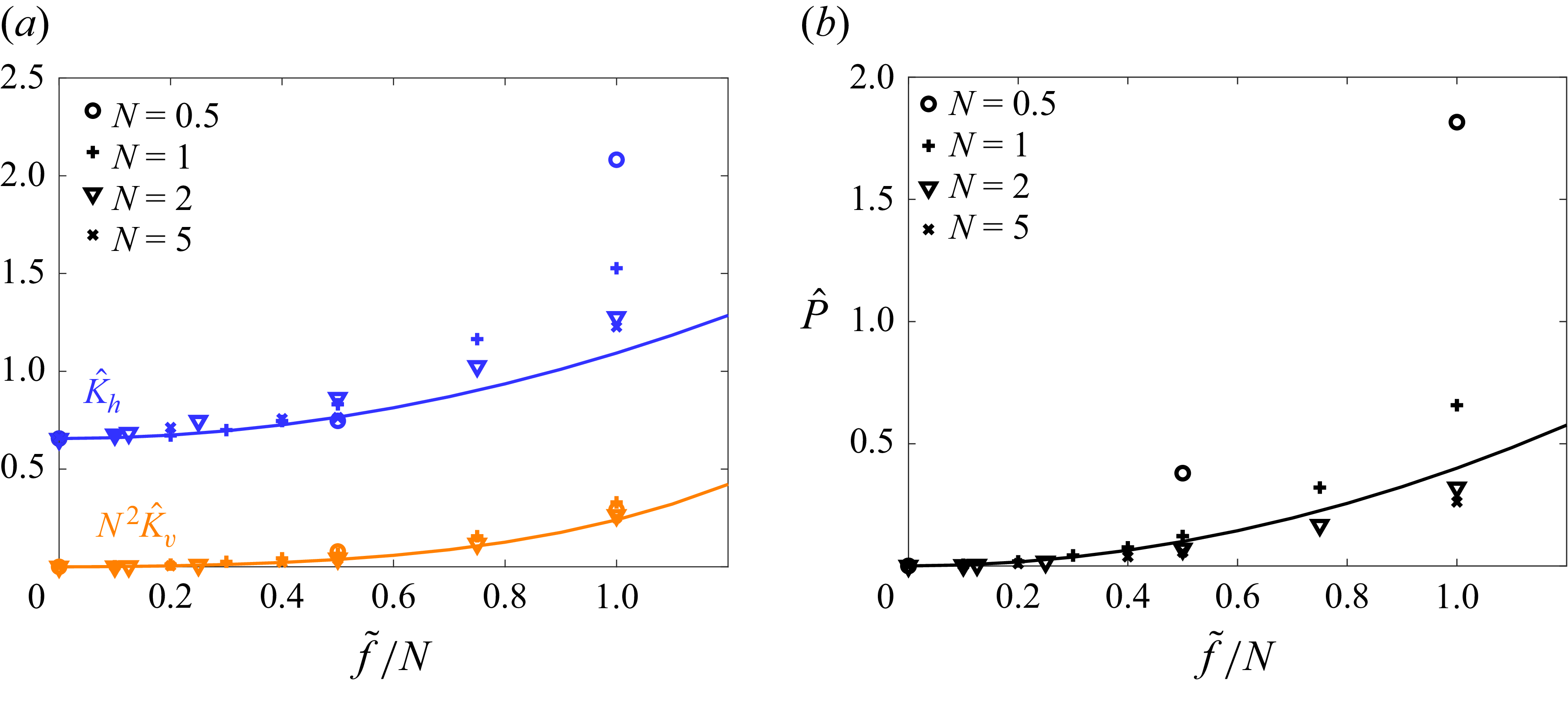
3.5.4. Summary of the scaling of the energies

The scalings for the three energies are summarised in figure 20. The symbols in this figure show the mean level at saturation of $\hat {K}_{h}$ , $N^{2}\hat {K}_{v}$ and $\hat {P}$ averaged over a range of $100$ time units after nonlinear saturation, as a function of $\tilde {f}/N$ for four values of $N$ . The solid lines represent the scaling relations derived in the strongly stratified limit for the three energies. The relation (3.22) for the horizontal kinetic energy is entirely given by the kinetic energy in the traditional limit $\hat {K}_{h}'\simeq 0.65$ and the ratio $\tilde {f}/N$ . In contrast, the multiplying factors in front of the relations (3.24) and (3.27) for the vertical kinetic energy and potential energy have been determined by a fit. These scaling relations are in good agreement with the simulations when $\tilde {f}/N$ is small and $N$ is large: $\tilde {f}/N\leqslant 0.5$ and $N\geqslant 2$ . On the other hand, some slight and significant departures exist for $N\geqslant 2$ and when $N\leqslant 1$ , respectively, for $\tilde {f}/N\geqslant 0.5$ , especially for $\hat {K}_{h}$ and $\hat {P}$ . This is expected because the assumption of a strongly stratified fluid used to compute these scaling laws is satisfied only when $N\gg 1$ .

Figure 20.

(a) Mean horizontal kinetic energy (blue) and vertical kinetic energy multiplied by $N^{2}$ (orange) at saturation as a function of the ratio $\tilde {f}/N$ . (b) Mean potential energy (black). The different symbols represent simulations at different $N$ . Solid lines show the relations $\hat {K}_h\simeq (1/3)(3+2(\tilde {f}/N)^{2})\hat {K}_h'$ (blue), $N^{2}\hat {K}_v\,=\,0.12(\tilde {f}/N)^{2}(1+(\tilde {f}/N)^{2})$ (orange) and $P=0.4(\tilde {f}/N)^{2}$ (black).