3.1.1. Large-scale structures

The AFM micrographs in Figure 3 show the large regular hillocks and valleys (large-scale spikes and bubbles) which resemble the top and bottom of the oscillating rectangular membrane (the “egg-carton” morphology) and the number of small-scale superimposed random spikes and bubbles. The wavelength of the large-scale spikes ranges from λ ≲ 45 µm in Figure 3a, to ~50 µm in Figure 3b, and to λ ~ 60 µm in Figure 3c. It may be attributed to the long-wavelength perturbation on the surface corrugation, d _scratch ~ 40–60 µm, indicating strong dependence on the initial conditions. The amplitude of the large spikes reaches ~(+) 1600 nm, and of bubbles ~(−) 600–700 nm in depth indicating approximately three times higher growth rates of spikes than of bubbles. This is in agreement with Alon et al. (Reference Alon, Ofer, Shvarts, Young, Glimm and Boston1966) that multi-mode RMI spike and bubble amplitude scale in different ways; the bubble amplitude h _B scales as h _B = α_B•t•Θ_B, where Θ_B = 0.4 at all A, while the spike amplitude h _S scales as h _S = α_S·t·Θ_S, where Θ_S depends on A, which does not appear in these relations (Alon et al., Reference Alon, Ofer, Shvarts, Young, Glimm and Boston1966). The α_B and α_S depend on the initial perturbation, and consequently the penetration of heavy fluid into the light fluid depends on the initial conditions at all times with A = 1. The spikes penetrate (at a constant velocity) as, h _S = α_S·t, (Θ_S = 1), as compared with Θ_B = 0.4 for the bubbles (Alon et al., Reference Alon, Ofer, Shvarts, Young, Glimm and Boston1966). Based on these relations one can explain why the growth of spikes in Figure 4a–4c is three times faster than in the case of bubbles (also in the region of a high density ratio, A ~ 1).

Fig. 3.

AFM micrographs of the CR showing the RMI structures. (a) Large-scale structures (hillock-valley) structures with λ ~ 45 µm, and superimposed small-scale structures. (b) Large-scale structures (hillock–valley) structures with λ ~ 50 µm, and superimposed small-scale structures. However, notice that there also appear the central hillock and valley which do not comprise any small-scale structure. (c) Large-scale structures (hillock–valley) structures with λ ~ 60 µm, and superimposed small-scale structures. Notice again, the central hillock and valley without any small-scale structure.

Fig. 4.

AFM micrographs showing a more detailed view of the central hillock and valley which do not comprise the small-scale structures. (a) Magnification of the large hillock (i) and the valley (ii) in Figure 3c reveals only a small surface irregularity. (b) Large micrograph of the hillock (i) and valley (ii) in Figure 4a reveals almost flat surface.

Consider the structures in Figure 3a–3c. One can see the central large-scale hillock (large spike) and valleys without any small-scale structure. At magnification, the large spike [Fig. 4a(i)] and bubble [Fig. 4a(ii)] show only small surface irregularities, possibly due to the fluid layer thinning. The layer thinning with tendency to zero-thickness does not enable the evolution of the small-scale RMI spikes and bubbles.

The large-scale “egg-carton” structures may be successfully compared with the large RMI structures numerically simulated assuming the single-mode (Miles et al., Reference Miles, Blue, Edwards, Greenough, Hansen, Robey, Drake, Kuranz and Leibrandt2005; Long et al., Reference Long, Krivets, Greenough and Jacobs2009) and the multi-modal perturbations Cohen et al., Reference Cohen, Dennevik, Dimits, Eliason, Mirin, Zhou, Porter and Woodward2002; Kartoon et al., Reference Kartoon, Oron, Arazi and Shvartz2003). An example are the large “egg-carton” structures obtained for the vertical interface oscillation in a square as a single-mode 3D perturbation

(1)$$z(x,y) = {a_0}\cos \,({k_x}x)\cos \,({k_y}y),$$

where a ₀ = 3.45 mm, k _x = k _y = √2 π/W, and W = width of the test section, for the weak shock of M _a = 1.22 and the low Atwood number A = 0.65 (Long et al., Reference Long, Krivets, Greenough and Jacobs2009).

The large hillock–valley structure – the “egg-carton interface” – was also obtained by Miles et al. (Reference Miles, Blue, Edwards, Greenough, Hansen, Robey, Drake, Kuranz and Leibrandt2005). They used multi-mode 3D perturbation and the “mode 4-run” given by z(x, y) = a ₀cos(k ₄x)cos(k ₄y), where k ₄ corresponds to the l = 4 mode. The perturbation amplitude was a ₀ = 2.5 µm, the Atwood number was A = 0.7, while the Reynolds number, Re,

(2)$$Re\; = \displaystyle{{hv} \over v}, $$

(h is the height of the vertical structure, v is the fluid velocity, and ν is the kinematic viscosity), varied in time reaching Re = 4400 at the end of pulse at t = 40 ns (Miles et al., Reference Miles, Blue, Edwards, Greenough, Hansen, Robey, Drake, Kuranz and Leibrandt2005).

The most complex 3D numerical simulation of RMI with a two scale initial perturbation which has given the regular egg-carton interface as well as the superimposed random small-scale structures – quite similar to our experimental ones – was performed by Cohen et al. (Reference Cohen, Dennevik, Dimits, Eliason, Mirin, Zhou, Porter and Woodward2002). The surface displacement at the interface for the membrane shocked through the grid was (Cohen et al., Reference Cohen, Dennevik, Dimits, Eliason, Mirin, Zhou, Porter and Woodward2002; Martin et al., Reference Martin, Taylor, Wu and Weirs2006; Schilling & Latini, Reference Schilling and Latini2010)

(3)$$z = {A_0}[ \vert \sin \,({k_x}) \vert \vert \sin \,({k_y}) \vert -\cos \,(2{\rm \pi} x)\cos \,(2{\rm \pi} y)],$$

where A ₀ is the non-dimensional perturbation amplitude A ₀ = 0.01 (A ₀ = a ₀/λ_p, λ_p is the perturbation wavelength), and k is the scaled wavenumber defined by k = k⊿ = 10π (k is the wavenumber in cm⁻¹ and ⊿ is the grid spacing in cm). The first term |sin(k _x)∣|sin(k _y) represents the small-scale perturbation associated with pushing the membrane through the wire grid. The second term cos(2πx)cos(2πy) which represents the perturbation associated with the transverse dimension of the shock tube scaled to have width of 2π (Cohen et al., Reference Cohen, Dennevik, Dimits, Eliason, Mirin, Zhou, Porter and Woodward2002; Schilling & Latini, Reference Schilling and Latini2010). The conjecture with our experiment is that the first term may indicate the local deformation of the target with the large-scale perturbation scratches (40–60 µm), while the second term indicates the perturbation of the fluid layer in the transversal direction of the rectangular spot. The numerical simulation performed at about 8 billion computational zones reveals the growth, organization of the RMI structures, and their subsequent mixing in non-dimensional time (Cohen et al., Reference Cohen, Dennevik, Dimits, Eliason, Mirin, Zhou, Porter and Woodward2002) (Figure 5). The Re number ranged from 1700 to 8000 indicating that the mixing transition occurs for a macroscale Re number of the order of 10⁴, in agreement with Dimotakis (Cohen et al., Reference Cohen, Dennevik, Dimits, Eliason, Mirin, Zhou, Porter and Woodward2002; Dimotakis, Reference Dimotakis2000). The variable plotted in Figure 5 is the entropy S chosen because it displays the contact discontinuity. The color mapping is chosen to be transparent red on the high density (low entropy and low temperature) side and transparent blue on the low-density side of the contact discontinuity (Cohen et al., Reference Cohen, Dennevik, Dimits, Eliason, Mirin, Zhou, Porter and Woodward2002). The formation of the large “egg-carton” spike/bubble structures with the superimposed small-scale ones, very similar to our micrographs in Figure 3a–3c, is clearly visible.

Fig. 5.

Numerically simulated growth of RMI and turbulent mixing. The variable plotted is the entropy S chosen because it displays the contact discontinuity. The color mapping is chosen to be transparent red on the high-density (low entropy, low temperature) side and transparent blue on the low-density side of the contact discontinuity. Notice the formation of the large-scale hillock–valley structures (spike/bubble structures) with the superimposed small-scale ones, similar to Figure 3a–3c. Courtesy of Dr. R.H. Cohen. Reproduced with permission from [Cohen et al., Reference Cohen, Dennevik, Dimits, Eliason, Mirin, Zhou, Porter and Woodward2002]. Copyright [2002], AIP Publishing LLC.

Regarding the small-scale structures in the micrographs (Fig. 3a–3c), we assume that they appear at the places where the liquid layer thickness is increased (interface thickening). The increase of the local fluid layer thickness resembles the local shock-induced flat membrane (interface) thickening in agreement with Vetter and Sturtevant (Vetter & Sturtevant, Reference Vetter and Sturtevant1995).

The random small-scale structures in Figure 3a–3c evolve from the incommensurate modes of the small scratch wavelength on the target surface (and of the eventual harmonics). The simulated small-scale structures in the shock tube evolve for the initial perturbation 2k/(2π) with the maximum allowed choice for k ~ 30 (Cohen et al., Reference Cohen, Dennevik, Dimits, Eliason, Mirin, Zhou, Porter and Woodward2002). As seen in Figure 5, they show very good regular organization for 1.5 ≥ t ~ 4.5, with the onset of randomization and turbulent mixing for t > 4.5 (Cohen et al., Reference Cohen, Dennevik, Dimits, Eliason, Mirin, Zhou, Porter and Woodward2002). Consequently, our small-scale structures in Figure 3a–3c which all are random and belong to the strong turbulent mixing, can be favorably compared with these “late time” small-scale structures for t > 4.5 (especially with those for t = 9), in Figure 5 of Cohen et al. (Reference Cohen, Dennevik, Dimits, Eliason, Mirin, Zhou, Porter and Woodward2002).

3.1.2. Small-scale spikes randomly organized

The analysis of the small-scale RMI spikes in Figure 3 can be started from their 2D topographic image in Figure 6a(i). The cross-section of the AFM data along the (white) line shows the variation of amplitude between h _S ≳ 200 and 220 nm (spikes), and h _B ~ (−) 80 nm (bubbles) [Figure 6a(ii)]. Comparison of the amplitudes of small spikes h _S and bubbles h _B indicates the slower growth rate of bubbles than spikes, h _B/h _S ~ 0.36–0.4 ~ 0.4 for the RMI, again in agreement with Alon et al. (Alon et al., Reference Alon, Ofer, Shvarts, Young, Glimm and Boston1966).

Fig. 6.

Characteristics of the RMI small scale structures. (a) 2D AFM topographic image of the structures in Figure 3a, (i); Section analysis along the white line in (i) shows variation of surface amplitude (ii); Histogram of the FFT modes (iii). Spectral amplitude rms = 0.308 nm. (b) 2D AFM topographic image of the structures in Figure 3c, (i); Section analysis along the white line in (i) shows variation of amplitude of spikes and bubbles (ii); Histogram of the FFT modes (iii). Spectral amplitude rms = 0.033 nm.

Considering the modes that take place in the RMI structure formation, the histogram of discrete 1D FFT in Figure 6a(iii) shows their relative amplitude versus frequency, ranging from DC (zero frequency) to Min (minimal frequency difference that can be resolved), along the section length. About ~30 Fourier modes have the amplitude which exponentially decreases to zero for N > 30, and the root-mean-square (rms) amplitude = 0.308 nm.

The 2D topographic image and the analysis of AFM data along the selected line in Figure 6b(i) – (that corresponds to Fig. 3a) – reveals the variation of amplitude between ~(–) 100 nm and ~(+) 150 nm and of the wavelength between λ ~ 5 and 8 µm [Fig. 6b(ii)]. The corresponding FFT histogram in Figure 6b(iii) shows an intermittent spectrum of modes with the amplitude which decreases from maximal to the zero value for N > 40. The rms amplitude = 0.033 nm, that is, one order of magnitude lower than in the case above.

3.1.3. Small-scale aperiodic spikes organized into wavy structures: The rows

The AFM analysis of patterns in Figure 3 – besides the domains of completely random small-scale spikes – reveals the domains of ~100 × 100 µm² in size with sharp spikes organized into wavy-like rows (Fig. 7a). Mostly asymmetric spikes, characteristic for the large A numbers (Long et al., Reference Long, Krivets, Greenough and Jacobs2009), are fully or partially merged along the rows. The rows are almost parallel to the Y-axis of the laboratory system, that is, they extend along the direction of the constant laser power distribution (Fig. 7b).

Fig. 7.

AFM micrograph of the RTI structures in the CR showing small-scale structures organized into rows. (a) The rows of spikes in the domain of ~100 × 100 µm². (b) The rows of spikes in the domain of ~55 × 35 µm².

3.1.4. Mixing and merging of aperiodic spikes along the rows

The analysis of rows indicates that mixing and merging and transition to turbulence dominantly occur along the Y-axis. It is known that the transition to turbulence occurs in the domains where the shear layers from individual spikes have merged, due to the process which is seeded by the small-scale incomensurate perturbation modes (Miles et al., Reference Miles, Blue, Edwards, Greenough, Hansen, Robey, Drake, Kuranz and Leibrandt2005). Assume, for the simplicity, that merging occurs only along the rows as a quasi-2D process without interaction with the neighbor rows. Thus, the size of the rows or the “chain-like domain” determines the size of the mixing zone. The length of the rows ranges from L ~ 100 to 150 µm, while their width is about W ~ 5 µm, so that the size of the mixing zone ranges from ≲500 to ~750 µm².

However, a detailed view of Figure 8a reveals that the rows are the irregular lines with slight lateral fluctuation (zigzag like) because the neighbor off-line-spikes (at the lateral distance equal or smaller than the half of the spike width), become also merged into the same row. It means that such lateral interaction of spikes increases the width of the mixing zone to W ~ 10–15 µm, so that the size of the mixing zone reaches ≲1000–2250 µm². According to Miles et al. (Reference Miles, Edwards, Blue, Hansen and Robey2004), the transversal merging may be connected with compressibility effects of the quasi-2D evolution of hydrodynamically unstable interfaces. In fact, for the high Mach numbers the pressure associated with kinematic drag on developing spikes can be sufficient to partially redirect spike growth into the direction transverse to the Y-axis (Miles et al., Reference Miles, Edwards, Blue, Hansen and Robey2004).

Fig. 8.

Mixing and merging of the sharp spikes in the segment of the length L ~ 8300 nm selected from the long row. (a) The AFM micrograph of the domain in the CR showing mixing and merging of sharp spikes. The rows are not perfect lines but the irregular ones, because the neighbor off-line-spikes (at the lateral distance equal or smaller than the half of the spike width), are also merged into the same row. The interval between the spikes (the segment length) is marked l ₁, l ₂,…,l _n, while the height of the segments (between the spikes) is marked h ₁, h ₂,…,h _n. (b) Diagram of the mixing and merging cycles of spikes, Δ versus Γ, along the segment L = 8300 nm, shown in Figure 8a. Notice that periods Δ = 1 and 2 are the stable periods, while all other periods (between them) are unstable. Behavior of the unstable cycles resembles the kicked oscillator which is pushed from the stable oscillation into the unstable one until it falls into the stable period again. Thus, the periods represent the limit cycles of the supercritical Hopf bifurcation.

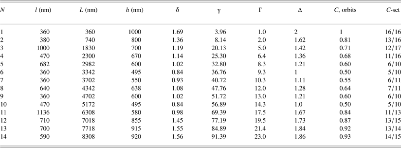
To analyze the mixing and merging process we select a short part of the length, L ~ 8300 nm, from the row; Figure 8a. The distance (segment) between the two spikes is marked by l ₁, l ₂, l ₃, _…, l _n (n = 1,…,14), and the corresponding height of the segments by h ₁, h ₂,…,h _n (Table 1). The average length of the segments “l” is assumed to be a quasi-period, λ (“l” =  λ = 590 nm), with the corresponding average wave vector k (k = 2π/λ = 6.28/590 = 0.011 nm⁻¹). From Figure 8a and Table 1, it follows that the ratio of the spike amplitude and the wavelength h _S/λ ~ 1–2 (h _S ≳ λ), indicating fast linear growth of sharp asymmetric spikes.

Table 1

Characteristics of merged spikes along the row in Figure 8a.

The length of the row of merged spikes, L ≂ 8300 nm; the average wavelength between the spikes “l” = λ=8300/14 ~ 590 nm; h, height of the interval of merged spikes; average wave vector “k” = 2π/λ = 6.28/590 ~ 0.011 nm⁻¹; L = l ₁ + l ₂ + · · · + l _n; Γ = γ/γ_min [γ = (L·k)/3.96, γ_min = 3.96]; δ = h/λ; ∆ = δ/δ_min (δ_min = 0.84); C, orbits shown as the fraction of period 2.

The insight into turbulent mixing is obtained from the ratio, δ_n (δ_n = h _n/λ ) in Table 1,  which reveals the repetition at δ_n = 1, δ_n = 24, δ_n = 6, and δ_n = 10, indicating cyclic nature of the process along the row. Better insight gives the set of ratios, ∆_n (∆_n = δ_n/δ_min; δ_min = 0.84), which shows that the system returns to the same value ∆_n = 1 and ∆_n = 24 as well as to ∆_n = 6 and ∆_n = 10 (which represent the steady states). These states may be identified as the stable periods P = 1 and 2. All other ∆-values represent the unsteady states, or the unstable cycles in the mixing process along the row.

Better insight into the mixing cycles along the row is obtained if the non-dimensional variable γ (γ_n = L _nk), is introduced. Normalizing γ to the minimal value (γ_min = 3.96) gets the new variable, Γ = γ/γ_min, what makes possible to present the diagram of mixing and merging cycles, Δ versus Γ (Fig. 8b). At Γ = 1, one finds the first stable period P ₁ = 2 which decreases intermittently through the unstable cycles until at Γ = 9.3 the cycle P ₂ = 1 is reached as the next stable period. With further increase of Γ, the cycle increases intermittently to P = 1.28 at Γ = 12, and then decreases reaching again P ₂ = 1 at Γ = 14.3. Beyond this value, the unstable cycle intermittently increases up to P = 1.86 at Γ = 23.0 and eventually comes to the stable period P ₁ = 2 at Γ > Γ₁₄. The behavior of the unstable cycles resembles the kicked oscillator which is pushed from the stable into the unstable oscillation until it falls into the stable period again (Table 1). Thus, the periods P = 1 and 2 represent the limit cycles of the Hopf bifurcation. Since all unstable cycles tend to the stable ones, the Hopf bifurcation is supercritical.

Expressing ∆_n as the fraction of the largest limit circle (P = 2), gives the Cantor set, C

(4)$$\eqalign{C = & \; 16/16,\,\,13/16,\,\,12/17,\,\,11/16,\,\,6/10,\,\,5/10,\,\,6/11, \cr & 7/11,\,\,6/10,\,\,5/10, 11/13,\,\,13/15,\,\,13/14,\,\,14/15, \ldots,} $$

which is not the Cantor fractal set because n is finite and short Table 1. However, one can assume that there exist many narrow spikes, which are also merged but cannot be distinguished due to limited resolution of the microscope. In that case, n is very large (it may be assumed n → ∞), and the set C becomes a fractal Cantor set. Obviously, the l _n and h _n become small, what has the consequence that δ_n tends to the same value (becomes constant) indicating – self-similarity – characteristic for the turbulent mixing process (Shvarts et al., Reference Shvarts, Sadot, Oron, Kishony and Srebro2000; Llor, Reference Llor2003). Therefore the self-similarity appears in CR where the spikes are arranged into rows.

3.1.5. Small periodic spikes inside the row of aperiodic spikes: No spike merging

In some long rows the periodic intervals of spikes appear inside the aperiodic ones (Fig. 9a). Their wavelength λ ~ 15–20 µm and the height h _s ~ 1000 nm [Fig. 9b(i, ii)] give the ratio h _S/λ = 0.05–0.07, (h _S ≪ λ), which indicates slow nonlinear growth. The sharp aperiodic spikes (at both sides of the periodic intervals) have h _s ~ 1000 nm and the wavelength λ ~ 7–10 µm, so that their ratio h _S/λ = 0.10–0.14, (h _S < λ), indicating faster growth. However, their growth although faster than of the periodic spikes is not as fast as in the case of the aperiodic spikes, considered above. One can say that the appearance of the periodic spike intervals – as the consequence of locally coherent flow – slows down the mixing process along the row. The periodic spike organization on the symmorphic pm11 symmetry group (Abarzhi, Reference Abarzhi2008) is characteristic for 2D flow (Y, Z) what is an argument in favor of our quasi-2D treatment of the spike organization into rows. In the other domains, the periodic segments of spikes are arranged in two parallel rows. The AFM in Figure 10a (side view) shows periodic spike segments (shifted one with respect to the other), that belong to the anti-simmorphic p2gm group (Fig. 10b), formed by the combination of translation and reflection (glide planes) (Abarzhi, Reference Abarzhi2008). Thus, the spikes inside the same row appear organized in two space groups, the symmorphic and the anti-symmorphic.

Fig. 9.

AFM micrograph of the domain of the CR showing the rows of spikes almost parallel to the Y-axis of the laboratory system. (a) The sharp spikes are symmetric and show the segments of periodic organization among the aperiodic ones. (b) Periodic spike organization (i), (ii) belongs to the same pm11 symmetry group characteristic for 2D flow.

Fig. 10.

AFM micrograph of the domain of the CR showing two parallel rows of spikes. (a) Two parallel rows of periodic spikes organized on the p2gm anti-symmorphic symmetry group. (b) Geometry of the p2gm symmetry group.

The space group G describes the symmetry operations of an organized structure consisting of a lattice which can be generated by successive translations of primitive vectors and a basis that may possess point-group operations: Rotations, inversions, and reflections (Liao, Reference Liao2012). The basic difference between these two space groups is that for a symmorphic space group all the translational and non-translational elements form the point group, which is a subgroup of the space group. For an anti-symmorphic space group, however, the non-translation elements do not form a subgroup of the space group (Liao, Reference Liao2012) (see Supplement B).

The effect of viscosity on the evolution of such RMI structures is expressed through the Reynolds number. Assuming the kinematic viscosity of light-fluid ν ~ 2 × 10⁻⁷ m²/s, the linear dimension of fluid motion due to vertical shock perturbation, h _s ~ 0.6–0.8 µm, and the velocity of the accelerated light-fluid v ~ 2100 m/s, one finds the Re number for the light-into-heavy fluid penetration, Re = h _sv/ν ~ 6.1 × 10³–8.4 × 10³, in good agreement with the Re numbers of Cohen et al. (Reference Cohen, Dennevik, Dimits, Eliason, Mirin, Zhou, Porter and Woodward2002) and Dimotakis (Reference Dimotakis2000).

Notice that in the qualitative sense the sharp RMI spikes for A ~ 1 and Re ~ 6.1 × 10³–8.4 × 10³ treated as the quasi-2D phenomenon, are in very good agreement with the sharp spikes obtained by Abarzhi and Hermann (Reference Abarzhi and Hermann2003) for the similar parameters A ~ 0.9, and Re = 6.97 × 10³ by 2D numerical simulation.

3.2.1. Discrete self-organization of mushroom-shape spikes

The AFM micrograph of the NCR in Figure 11a of ~100 × 100 nm² in size shows quite different shape of RTI spikes. The symmetric spikes – characteristic for the lower A numbers (Long et al., Reference Long, Krivets, Greenough and Jacobs2009) – are not organized into rows except those in some smaller domains. In the NCR, the transition to mixing occurs in a different way than in the CR due to formation of correlated flow field in localized domains.

Fig. 11.

AFM image of the domain of the NCR showing the small-scale structures organized on 2D lattice in the (X, Y)-plane. (a) Domain of the size ~100 × 100 µm². (b) Characteristics of the small-scale structures. (i) 2D AFM topographic image of the structures in Figure 11a; (ii) section analysis along the white line in (i) shows variation of amplitude of spikes and bubbles; (iii) Histogram of the FFT modes along the white line in (i). Spectral amplitude rms = 0.006 nm.

The 2D topographic image and the cross-sectional analysis of the AFM data along the selected line in Figure 11b(i) show the surface variation between ~(–) 100 and ~(+) 200 nm and of the wavelength between λ ~ 3.5 and ~10 µm [Fig. 11b(ii)]. General observation is that in the NCR the horizontal scale of the small structures grows much faster than the vertical one. The corresponding FFT histogram shows an intermittent spectrum of modes with the amplitude which decreases from maximum to the zero value for N > 20 [Fig. 11b (iii)]. Spectral amplitude rms = 0.006 nm, that is, it is extremely small and does not have any influence on the linear growth saturation.

Different type of the spike shape and organization as the result of 3D flow correlated in the (X, Y)-plane, is observed in the smaller domains of the NCR. An example is the domain of ~10 × 10 µm² in size with thick mushroom-shape spikes of the height h _S ~ 0.2–0.3 µm and the period, λ₁ = λ₂ = λ ~ 3.2 µm (Figure 12a). The corresponding isotropic square lattice (p4mm) has the inversion point and is therefore a stable structure (Abarzhi, Reference Abarzhi1998; Reference Abarzhi2008). The ratio h _S/λ ~ 0.06–0.09, (h _S ≪ λ), indicates slow nonlinear growth of spikes. Notice that the dark concave-spaces (between the mushroom-shape spikes) indicate bubbles (of upper light fluid growing into the lower dense fluid). The bubbles are almost flat – the phenomenon which occurs in the late phase of the RMI/RTI (Abarzhi et al., Reference Abarzhi, Nishihara and Glimm2003).

Fig. 12.

Domain of the NCR showing the mushroom-shape spikes organized on 2D lattice in the (X, Y)-plane. (a) AFM image of the domain ~ 10 × 10 µm² (square lattice), λ₁ ~ 3.2 µm, λ₂ ~ 3.2 µm. (b) AFM image of the domain ~ 10 × 10 µm² (rhombic lattice), λ₁ ~ 3.2 µm, λ₂ ~ 3.2 µm. (c) Organization of the mushroom-shape spikes on the square and the rhombic lattices with the c4mm and cmm symmetry groups, respectively (transformation between the lattices).

The transformations of organization of the mushroom-shape spikes in the inhomogeneous flow field occur independently in the local domains. The domain in Figure 12b shows spikes organized on the (cmm) rhombic lattice with the same period (λ₁ = λ₂ ~ 3.2 µm) as of the rectangular one in the case above. The dark, slightly concave spaces between the spikes are flat bubbles. The transformation between two latices is shown in Figure 12c.

Figure 13a(i) of the domain of ~20 × 20 µm² in size shows the mushroom-shape spikes organized on the lattice (λ₁ ~ 6.5 µm, and λ₂ ~ 9.5 µm) that belongs to the p2 symmetry group [Fig. 13a(ii)]. Again, the dark spaces (which seem more curved than in the case above), are the flattened bubbles (Abarzhi et al., Reference Abarzhi, Nishihara and Glimm2003).

Fig. 13.

Domain of the NCR showing the mushroom-shape spikes organized on 2D lattice in the (X, Y)-plane. (a) AFM image of the domain ~20 × 20 µm² with λ₁ ~ 6.5 µm, λ₂ ~ 9.5 µm (i); Organization of the mushroom-shape spikes on the rhomboid lattice with p2 symmetry group (ii). (b) AFM image of the domain ~ 40 × 40 µm² with λ₁ ~ 9.5 µm, λ₂ ~ 13 µm (i); Organization of the mushroom-shape spikes on the rhomboid lattice with p2 symmetry group (ii).

Figure 13b(i) of the domain of ~30 × 30 mm² in size shows the mushroom-shape spikes organized on the periodic lattice (λ₁ ~ 9.5 µm, and λ₂ ~ 13 µm), which also belongs to the same p2 symmetry group and represents the stable structure [Fig. 13b(ii)]. Since the height of the spikes, h _S ≲ 1.0 µm, the ratio h _S/λ ~ 0.07 indicating a slow nonlinear growth of spikes. Notice that some of the bubbles are only slightly curved (almost flat), whereas the others (dark ones) are more curved and deeper. In a qualitative sense, the 3D flattening of the bubble surface in Figures 12 and 13 can be favorably compared with the bubble curvature obtained by numerical simulation of Abarzhi and Hermann (Reference Abarzhi and Hermann2003), although their simulation is 2D.

According to Abarzhi et al. (Reference Abarzhi, Nishihara and Glimm2003), the bubble curvature and velocity in RMI, change and in the linear regime their curvature reaches the extreme value, dependent on the initial conditions. As t/τ_RM → ∞ the bubble flattens and decelerates. For A < 1, the bubbles move faster than those for A = 1, and for A ≤ 1 the bubbles are flat. The flattening of the bubble front is a distinct feature of RMI universal for all A (Abarzhi et al., Reference Abarzhi, Nishihara and Glimm2003).

The horizontal scales λ₁ and λ₂ increase from Figures 12 to 13. The selection of scales is a result of the horizontal flow field which transforms the isotropic lattice into the anisotropic. The fluid acceleration is inhomogeneous and the organization of mushroom-shape spikes in various domains has different lattice periods λ₁ and λ₂. The isotropic square lattice in Figure 12 (p4mm) with λ₁ = λ₂ = λ ~ 3.2 µm is transformed into the rhombic one (cmm) with the same period λ. The rhomboid structure (p2) in Figure 13a, has λ₁ ~ 6.5 µm (which is ~2λ), and l₂ ~ 9.5 µm (which is just ~ 3l). Also, the structure in Figure 13b, has λ₁ ~ 9.5 µm which is ~3λ, whereas λ₂ ~ 13 µm which is just 4λ. Therefore, the lattice periods λ₁ and λ₂ become two, three, or four times larger indicating formation of superstructure with double, triple, or quadruple lattice size (Abarzhi et al., Reference Abarzhi, Nishihara and Glimm2003). Characteristic of the isotropic turbulence is that the local momentum is balanced (M_local = 0), while the time- and scale-invariance of the energy dissipation rate is comparable with the inertial interval and non-dissipative energy transfer between the scales (Abarzhi & Rosner, Reference Abarzhi and Rosner2010). In accelerated turbulent mixing, the local momentum is imbalanced (M_local ≠ 0), and time- and scale-invariance imply that at any time and length scale the specific momentum is being lost at the same constant rate, and momentum transfer between the scales is non-dissipative (Abarzhi & Rosner, Reference Abarzhi and Rosner2010).

Assuming for the NCR, the kinematic viscosity of light-fluid ν ~ 10⁻⁷ m²/s, the velocity of the accelerated light-fluid v ~ 2100 m/s, the height of linear dimension of fluid motion is, h _s ~ 0.35–0.50 µm, one finds the Re number for the light-into-heavy fluid penetration, Re ~ 7.35 × 10³–1 × 10⁴, that is, or Re ~ 10⁴.