Parties, Coalitions, and the Internal Organization of Legislatures

DANIEL DIERMEIER; RAZVAN VLAICU

doi:10.1017/S0003055411000104

Parties, Coalitions, and the Internal Organization of Legislatures

Published online by Cambridge University Press: 18 May 2011

DANIEL DIERMEIER and

RAZVAN VLAICU

Show author details

DANIEL DIERMEIER*: Affiliation:
Northwestern University
RAZVAN VLAICU*: Affiliation:
University of Maryland
*: Daniel Diermeier is IBM Professor of Regulation and Competitive Practice, Kellogg School of Management, Northwestern University, and Director of the Ford Center for Global Citizenship, 2001 Sheridan Road, Evanston, IL 60208 (d-diermeier@kellogg.northwestern.edu).
Razvan Vlaicu is Assistant Professor, Department of Economics and Affiliate, Department of Government and Politics, University of Maryland, 3105 Tydings Hall, College Park, MD 20742 (vlaicu@econ.umd.edu.).

Article contents

Abstract
PREFERENCES: PARTIES AS GROUPS OF LIKE-MINDED LEGISLATORS
LEGISLATIVE DECISION MAKING
LEGISLATIVE BEHAVIOR
DISCUSSION
CONCLUSION
Footnotes
References

Rights & Permissions

Abstract

We present a theory of parties-in-legislatures that can generate partisan policy outcomes despite the absence of any party-imposed voting discipline. Legislators choose all procedures and policies through majority-rule bargaining and cannot commit to vote against their preferences on either. Yet, off-median policy bias occurs in equilibrium because a majority of legislators with correlated preferences has policy-driven incentives to adopt partisan agenda-setting rules—as a consequence, bills reach the floor disproportionately from one side of the ideological spectrum. The model recovers, as special cases, the claims of both partisan and nonpartisan theories in the ongoing debate over the nature of party influence in the U.S. Congress. We show that (1) party influence increases in polarization, and (2) the legislative median controls policy making only when there are no bargaining frictions and no polarization. We discuss the implications of our findings for the theoretical and empirical study of legislatures.

Information

Type: Research Article
Information: American Political Science Review , Volume 105 , Issue 2 , May 2011, pp. 359 - 380
DOI: https://doi.org/10.1017/S0003055411000104 [Opens in a new window]
Copyright: Copyright © American Political Science Association 2011

The debate over the role of parties in the U.S. Congress is as old as the modern study of Congress itself. Although classic texts such as David Mayhew's (Reference Mayhew1974) Congress: The Electoral Connection had previously questioned the role of parties in congressional politics, it was the publication of Keith Krehbiel's (Reference Krehbiel1993) “Where's the Party?” that reignited the debate, leading to scores of articles and books. Yet, the debate does not appear to be abating in the slightest (e.g., Smith Reference Smith2007; Rohde, Stiglitz, and Weingast Reference Rohde, Stiglitz and Weingast2008). In part, this may be due to the fact that parties are among the more complex political institutions, closely connected to both legislative and electoral politics that, as research domains, usually progress in isolation from each other.

The key question underlying the debate is, simply put, whether parties are able to affect legislative outcomes above and beyond what legislators would choose if they acted independently, without party direction. This test of “party influence” was articulated in Krehbiel (Reference Krehbiel1993) and has been widely accepted.Footnote ¹ Furthermore, based on empirical (Krehbiel Reference Krehbiel1995) and theoretical (Krehbiel Reference Krehbiel1991, Reference Krehbiel1998) work, he has argued that it is legislators' policy preferences, rather than their partisan affiliations, that drive legislative outcomes. Party structures cannot make voting behavior more partisan than what can be predicted from individual preferences alone. In particular, even if we observe that the majority party controls legislative institutions, because these institutions are subject to majority rule approval, they must reflect the preferences of a majority of the legislature (i.e., the median legislator). This view of “weak parties” is known as the pivotal politics model (PPM).

Over the same period, “partisan” theories were developed that, in contrast to the PPM, make the case for partisan affiliations, and not strictly individual interests, being the critical variable driving legislative outcomes. Two variants of partisan theories can be distinguished. Cox and McCubbins (Reference Cox and McCubbins2005, 19) clearly state the distinction:

Parties as floor voting coalitions. Some partisan theories view parties primarily as floor voting coalitions. In such theories, the central issue is the degree to which parties can discipline their members, ensuring a cohesive voting bloc on the floor, even when there are internal disagreements over policy.

Parties as procedural coalitions. Other partisan theories, including our own, view parties primarily as procedural coalitions. For such theories, the central issue is the majority party's ability to control the legislative agenda, defined as the set of bills considered and voted on the floor.

The first variant (“floor voting coalitions”) is usually based on a public good argument. Forming a legislative coalition provides various collective benefits to members. Because these may conflict with individual interests, however, a collective action problem arises. Coalition-preserving behavior needs to be enforced through selective incentives. For example, party leaders can use appointments to attractive committees or allocations of staff resources to win a member's loyalty. Conditional party government (CPG) theory (Aldrich and Rohde Reference Aldrich, Rohde, Dodd and Oppenheimer2001; Rohde Reference Rohde1991) and endogenous party government theories (Patty Reference Patty2008; Volden and Bergman Reference Volden and Bergman2006) adopt this approach.

CPG further claims that party influence is not fixed, but increases with intraparty ideological cohesion and interparty ideological distance. Although making an empirically plausible claim, CPG is based on a premise that PPM rejects on theoretical and empirical grounds: namely, that party leaders can effectively pressure party members to change their votes on policy issues.Footnote ²

The second variant (“parties as procedural coalitions”) avoids this issue by conceptualizing party influence as an agenda control problem. Instead of pressuring members to toe the party line on policy issues, party leaders take control of procedures that can influence the agenda, such as a policy committee with gatekeeping power or a committee that sets the terms of debate (e.g., the Rules Committee in the U.S. House of Representatives). The consequence is that even if legislators vote on policy unconstrained, as in PPM, there would be bias in policy outcomes because party leaders can control which issues can be brought to a vote.

How does the majority party take control of the agenda? Procedural cartel theory (PCT) argues that the party leadership is able to enforce voting discipline over procedural issues (Cox and McCubbins Reference Cox and McCubbins2005). Procedural voting discipline can be enforced because in exchange the party provides collective goods: Party members care not only about policy, but also about a collective good such as their party's reputation with the electorate. Thus, they give the majority party leadership control of the agenda to keep party-splitting issues away from the floor because lack of voting cohesion on the floor will blur the party's image with voters. Bending under this indirect type of party pressure is also less electorally costly for party members because the arcane details of the legislative process are less transparent to their constituents.Footnote ³

This type of procedural voting discipline is ruled out by PPM as not enforceable in a legislature whose procedures are chosen by majority rule. Krehbiel (Reference Krehbiel2004, 117) puts it this way:

Majoritarianism and procedural endogeneity imply that the median voter is pivotal in a procedurally neutral setting. Why would such a legislative voter consent to procedures whose foreseeable consequences are tantamount to an abdication of power?

In other words, PPM views legislative procedures as subject to the same voting rules as regular policies. Policy preferences will induce preferences over procedures. Because the median is pivotal over policy, it will also be pivotal over procedures. Therefore, the median, not parties, controls procedures.

In this article, we theoretically identify a type of party influence that does not hinge on the existence of party discipline on either policy or procedural issues.Footnote ⁴ We show that party leadership pressure is not necessary for parties to matter. Party-induced policy bias can also occur because a majority of like-minded legislators, in pursuing their individual policy preferences, freely vote to form an agenda-setting coalition that limits floor amendments.

We formalize this argument in a model with two features: (1) all policy issues are one dimensional and preferences are single peaked, and (2) all legislative decisions (procedural and policy) are made through unconstrained majority-rule bargaining on the floor (i.e., not in party caucuses or dictated by party leaders).Footnote ⁵ Yet, the equilibrium is not the median on every issue.

Off-median deviations arise in equilibrium because of bargaining frictions (e.g., opportunity costs). Moreover, if the legislature features preference polarization into two types, then policy outcomes are systematically biased away from the median. The reason is the noncooperative capture of agenda control by a legislative coalition that shares similar preferences—with the consequence that bills reach the floor disproportionately from one side of the ideological spectrum.

Specifically, our model produces three formal results. These results shed light on the three major theories of parties-in-Congress mentioned previously. We first show how opportunity costs and polarization create equilibrium deviations from the median through agenda control (cf. PCT). The second result is that party influence increases with polarization (cf. CPG). Finally, we uncover the conditions under which the median, rather than the majority party, controls policy making: zero opportunity costs and lack of preference polarization (cf. PPM).

The basic intuition behind these results is as follows. Modern legislative bodies have two major features: first, they face time constraints, in the sense that deliberating on one issue entails the opportunity cost of leaving other issues unaddressed; and second, they use a legislative protocol of proposals (bills), amendments, and votes for decision making. In such an environment, making a first proposal gives the proposer a bargaining advantage because other legislators may find it costly to amend the proposal. Thus, agenda power becomes a valuable resource, and legislators will have incentives to restrict access to it.

In particular, when the legislature contains a majority of like-minded legislators (i.e., who are more likely to be on the same side of any given policy issue), they will have incentives to form an agenda-setting coalition because they can benefit from each other's bargaining advantage on specific issues. Even if sometimes they will be on opposite sides of the same issue, on average, all like-minded majority members benefit from sharing agenda control. As a legislature becomes more polarized, rendering the majority more consistently on the same side of issues, the agenda-setting coalition will vote to tighten its agenda control further, for instance, by limiting amendments. This will push policy outcomes further on the majority's side, increasing policy bias (i.e., average off-median policy deviations). Voting over policy becomes more cohesive as well.

Policy bias disappears only when polarization dissipates. Without polarization, legislators prefer median policies, and so will want to keep amendments unrestricted. Policy still deviates from the median, however, because of bargaining frictions caused by opportunity costs. In other words, the legislative median will prevail (PPM) only for zero opportunity costs and no polarization.

A noteworthy feature of our model is that it encompasses as special cases the predictions of all three major theories of Congress. Thus, the immediate benefit of the model is that it demonstrates that, although the premises of the three theories may appear contradictory, their claims can be reconciled under certain conditions. Our results suggest that, rather than being viewed as competing, mutually exclusive, theories, each approach may be understood as correctly identifying a different, yet equally important, determinant of legislative policy making. These are: individual preferences, partisan preferences, and agenda power. Importantly, our model uncovers the factors that control when each of these three determinants becomes dominant: opportunity costs and ideological polarization.

Perhaps the most important insight of the model is that party influence is possible without party discipline.Footnote ⁶ The type of party influence we uncover works through a previously unrecognized channel: majoritarian policy-seeking legislative organization. This result has theoretical and empirical repercussions.

Theoretically, we believe our analysis suggests a more nuanced understanding of the term “majoritarianism” and a reconsideration of the question of whether institutions such as the U.S. House of Representatives are majoritarian (see Patty Reference Patty2007). Our model features “procedural majoritarianism” because procedures are chosen using majority rule, without other constraints. However, as we show, that does not prevent off-median policy bias from occurring. In this sense, “procedural majoritarianism” does not necessarily lead to “policy majoritarianism.”

Empirically, our formal claims should assist researchers in developing new identification strategies to measure party influence. For instance, our findings imply that strategies that rely on party leadership pressure as the only gauge of a party effect (e.g., Snyder and Groseclose Reference Snyder and Groseclose2000) may be underestimating the full extent of party influence. Our comparative statics results characterize how party influence should vary with polarization and opportunity costs. These results can further assist in specifying empirical models of party effects.

We start by presenting our model of preferences and decision making, followed by the formal results. We close by discussing the theoretical and empirical implications of our results, followed by a brief conclusion. Proofs of all formal results are presented in the Appendix.

PREFERENCES: PARTIES AS GROUPS OF LIKE-MINDED LEGISLATORS

We start building our formal model on Krehbiel's concept of “weak parties” (i.e., the view that a party is simply a happenstance collection of legislators who are more likely than not on the same side of policy issues).Footnote ⁷ Legislative institutions, selective incentives, or agenda control play no role (Krehbiel Reference Krehbiel, Weingast and Witman2006a). This is our model of preferences. In the next section, we study how preferences translate into policy outcomes. As we see, this critically depends on the model of policy-making: the underlying process for bringing up policy alternatives to a vote.

Issue Preferences

We formalize Krehbiel's position using the standard spatial model with single-peaked preferences. Assume a majority-rule legislature consisting of 2k+1 members, where k is a positive integer.Footnote ⁸ Denote the set of legislators by N.

The legislature makes policy on a number of one-dimensional issues. For each issue s, a policy alternative p _s is a real number in the interval [−k, k]. On issue s, legislator i has an “ideal” point p _sⁱ. His preferences over alternatives p _s in [−k, k] are represented by the following utility function:

(1)

$\begin{equation} u_{i}(p_{s})=v\left(\left \vert p_{s}-p_{s}^{i}\right \vert \right), \end{equation}$

where v is twice continuously differentiable, strictly decreasing, strictly concave, v′(0) = 0 and v(2k) ≥ 0. Note that these assumptions imply that u _i is symmetrically single peaked at ideal point p _sⁱ.Footnote ⁹

On each policy issue, legislators' ideal points are the integers {−k, −k+1, . . .,−2,−1, 0, 1, 2,. . ., k−1, k}. These ideological “locations” can change from issue to issue according to the model in the next subsection.

We choose this particular policy environment for three reasons. First, it can represent Krehbiel's argument because the median is well defined on every policy issue. A second advantage is that it readily exposes how opportunity costs and agenda setting can affect the majority-rule equilibrium: The effect can be measured simply by the size of deviations from the median. Third, because majority rule yields a clear outcome on each policy issue, the role of parties in our model is not to “create order out of multidimensional chaos” by performing a coordination function, as Aldrich (Reference Aldrich1995) argues. Rather, it is to create policy deviations from the median that systematically favor all party members.

Preference Polarization

We now formally represent the notion of parties as “like-minded legislators.” Our model captures the common intuition that a legislator may slide on the left–right ideological spectrum depending on the issue at stake, but that members of the same party are more likely to be on the same side of an issue.Footnote ¹⁰

The simplest way to model this intuition is to assume that there are two preference types and two issue types. Denote the two preference types (parties) by A and B, and assume that party A has a simple majority (k+1 vs. k).Footnote ¹¹ Denote the two groups N _A and N _B.

We define a policy issue as a particular ordering of ideal points. Thus, with 2k+1 legislators, there are (2k+1)! different possible policy issues. We distinguish between two issue types: separated and mixed. A policy issue is separated if all As are on the left of the issue median, and all Bs on the right.Footnote ¹² A policy issue is mixed if at least one A type is on the right of the issue median. We assume that all separated issues are equally likely, and all mixed issues are equally likely, but that a separated issue is at least as frequent as a mixed issue. This creates the needed correlation: As are more likely to be on the left of an issue, and Bs more likely on the right.

Let π denote the aggregate frequency of separated issues for this legislature. The frequency distribution of policy issues in then

(2)

$\begin{equation} f(s)=\left \{ \begin{array}{@{}l@{\hspace*{10pt}}l@{}} \frac{\pi} {k!(k+1)!}, & \text{if issue} s\text{is separated}\\ \frac{1-\pi} {(2k+1)!-k!(k+1)!}, & \text{if issue} s\text{is mixed.} \end{array}\right. \end{equation}$

If π =1, then the legislature is completely polarized: On all issues, all As oppose all Bs. At the other end of the spectrum, when $\pi =\frac{k!(k+1)!}{(2k+1)!}$ , all issues are equally likely; in particular, a separated issue is as frequent as a mixed issue, so there is no polarization. Intermediate levels of polarization occur when $\frac{k!(k+1)!}{(2k+1)!}$ < π < 1.

Note that in this model of polarization, “like-mindedness” is captured through a form of distributional homogeneity: ex ante, all members of a preference type have the same marginal distribution of ideal points over policy issues; while ex post, no two legislators, even within a preference type, have the same ideal point. This implies that partisan voting cohesion on policy proposals can be low.

A technical virtue of this model of preferences is that “polarization” can be measured with a one-dimensional parameter π. This is important because our goal is to analytically derive the equilibrium effect of polarization on legislative organization.Footnote ¹³ A richer model of preferences that could accommodate alternative versions of partisan polarization may require multidimensional parametrizations, which would complicate the model's solution and obscure the comparative statics. As we see, the logic of the model does not require this particular form of ex ante homogeneity within a party. In a latter section, we explore weaker forms of preference affinity: different marginal distributions, but same expected ideal point: and different expected ideal points, but same support. These cases produce an equilibrium policy bias similar to the main model.

We also chose this model of polarization to clearly distinguish our arguments from existing partisan theories of legislative organization. First, because there are no natural “leaders” within a preference type that could function as centers of gravity around which the party rallies, any form of party influence has to arise out of majority members' individual preferences. This is in contrast to the partisan theories of Cox and McCubbins (Reference Cox and McCubbins2005) and Patty (Reference Patty2008), where party influence is based on the existence of a “party leadership” or party caucus that is empowered by members to, if necessary, alter the members' policy votes or procedural votes. Second, our model of polarization stresses one of the major points of this article: that party strength is rooted in affinities in individual policy preferences rather than common goals such as the party “brand” (Cox and McCubbins Reference Cox and McCubbins1993), protecting the party record by minimizing the party's roll rate (Cox and McCubbins Reference Cox and McCubbins2005), or pursuing a partisan agenda (Patty Reference Patty2008).

In what follows, we augment this preference model with a policy-making model with endogenous agenda-setting rules. We see how in this policy-making environment opportunity costs create policy deviations from the median. Are these off-median deviations random or systematically falling on the same side of the median? What are the incentives to sustain these deviations through agenda-setting rules? What controls the strength of these incentives?

LEGISLATIVE DECISION MAKING

What does the preceding model of preferences imply about policy making? That depends on the underlying process that brings up policy alternatives to a vote. We consider two: a majoritarian legislature and a “busy” legislature.

Majoritarian Legislature

Suppose that all legislators have equal procedural and voting power and that proposals and amendments can be made without cost until an alternative is found that cannot be beaten by majority rule (see Austen-Smith and Banks Reference Austen-Smith and Banks2000). In this purely “majoritarian” environment, legislative institutions are irrelevant, and policy is driven exclusively by individual policy preferences. Because on each policy issue there is a median, and voting is by majority rule, each issue median will successfully pull policy to its preferred location.

Define policy bias as the average (across issues) deviation between equilibrium policy p*_s and the median: p* = ∑_sp*_sf(s). We use policy bias as a summary measure of party influence because it averages the party's effect over all policy issues.

Proposition 1. Under majoritarian policy-making, equilibrium policy on all issues s is the respective issue median p*_s = 0. Equilibrium policy bias is, therefore, zero.

With this result in mind, we can now state the core of Krehbiel's (Reference Krehbiel, Weingast and Witman2006a, Reference Krehbiel2006b) critique against “parties as procedural coalitions.” It goes as follows:

1. The notion of agenda control presupposes control over legislative institutions.
2. In a majoritarian legislature, control over legislative institutions depends on support of the chamber majority (the “median voter”).
3. Therefore, policy outcomes cannot be biased away from the median because the median could otherwise simply change the organizational structure to eliminate the bias.

The structure of Krehbiel's argument seems compelling. Because the chamber as a whole chooses policy, it must be in the chamber's interest to rectify any deviation from the median's ideal point on a given policy by adjusting the procedural context. For example, if committees keep the gates closed and frustrate a chamber majority that would like to consider the bill on the floor, then why would the floor not simply vote on a discharge procedure? If the exact details of the discharge procedure are too onerous, then why not change them to make it easier for the chamber majority to obtain its preferred outcome?

In other words, legislative procedures are just more or less complicated choice alternatives subject to the same voting rules as votes on policies. Policy preferences will induce preferences over institutional arrangements. Therefore, Krehbiel argues, there can be no gap between majorities on policies and majorities on procedure.

In our view, the implicit assumption in Krehbiel's approach is that generating policy alternatives and voting on them are essentially costless activities. Indeed, as we show, this is a necessary condition for Krehbiel's argument to hold. However, what if procedural costs are nonnegligible?

A “Busy” Legislature

Perhaps the most plausible rationale for procedural costs is the “plenary bottleneck” argument (Cox Reference Cox, Weingast and Wittman2006; Cox and McCubbins Reference Cox and McCubbins2005). It is based on the following premises:

1. Bills can only be passed pursuant to formal motions and voting in plenary session. This process necessarily takes some amount of time.
2. Bills pass if a majority votes for them.
3. The plenary session faces a hard time constraint.

Premises (1)–(3) seem uncontroversial.Footnote ¹⁴ Together, they imply that a vote on any given bill is subject to an opportunity cost. That is, the time spent on any given bill could be used to debate or decide on some other issue. Cox (Reference Cox, Weingast and Wittman2006) argues that these time constraints are substantialFootnote ¹⁵; in other words: too many bills, too little time. We can formally represent this idea with the following model of legislative decision making.

Timing. Consider a legislature that chooses not only policy, but also the procedures through which a policy is adopted. The legislature makes first procedural and then policy choices using the same basic “random proposer” bargaining protocol (Banks and Duggan Reference Banks and Duggan2000) under majority rule. The timing of this protocol is as follows:

1. An agenda setter is randomly selected from a previously determined coalition C ⊆ N to make a proposal.
2. All legislators simultaneously vote on the proposal.
1. a. If a majority votes in favor, then the proposal is adopted and bargaining ends.
2. b. If the proposal does not receive a majority of votes, then bargaining ends with probability γ (due to opportunity costs) and all legislators receive a zero payoff.Footnote ¹⁶
3. If bargaining continues, then:
1. a. With probability x amendments can be made. Any legislator in N can be recognized to make an amendment.
2. b. With probability 1 − x, bargaining stops and all legislators receive a zero payoff.
4. If an amendment has been made, then all legislators simultaneously vote on the amendment.
1. a. If a majority votes in favor, then the amendment is adopted and bargaining ends.
2. b. If the amendment does not receive a majority of votes, then bargaining ends with probability γ (due to opportunity costs) and all legislators receive a zero payoff.
5. Step 3 is repeated.

Legislators use this protocol four times to make four choices in this sequence: (1) coalition size c, (2) coalition members C = {i ₁, . . ., i _c}, (3) amendment power x, and (4) policy p _s.Footnote ¹⁷

The first three choices (c, C, x) define the agenda-setting rules or procedures that will govern subsequent policy choices. They are chosen under uncertainty about what policy issues will arise in the legislative session. Once procedures are in place, legislators use them to choose policies p _s.

Although the basic bargaining protocol is common to both procedural and policy choices, the parameters of the protocol may differ in equilibrium between procedural and policy issues. Specifically, we exogenously impose that the three procedural choices are made under neutral procedures. In contrast, policy choices can possibly be made under restricted procedures, if the legislature so decided. By neutral procedures, we mean that all legislators can be recognized, with equal probability, to make a proposal (i.e., C = N), and amendments are unrestricted x = 1. Under restrictive procedures, only a subset of legislators may be recognized to make a proposal—the members of a coalition C ⊆ N—and amendments may be allowed only some of the time x < 1.

Equilibrium Concept. We characterize strategy profiles that are sequentially rational. Each bargaining game has two types of strategies: proposal strategies and voting strategies. For proposal strategies, we require two conditions: first, proposal strategies are stationary (i.e., are independent of the history of play up to the current period); second, stationary strategies are no-delay in the sense that setters make only proposals that a majority prefers to waiting.Footnote ¹⁸ For voting strategies, we require that they be weakly undominated.Footnote ¹⁹ We also require that, in each bargaining game, equilibrium strategies yield equal ex ante payoffs to players who at the beginning of the bargaining game are strategically equal. This condition implies that we are looking for strategy profiles that are symmetric relative to the strategic environment. Finally, if a bargaining game has multiple equilibria, then we select the ones in pure strategies.

Discussion. Notice the following features of the model. First, legislators choose organization in a procedurally neutral environment (i.e., all legislators have equal agenda power and equal voting power). This is our major departure from PCT. Because our model rules out party discipline at the organizational stage, the adopted rules must reflect individual majoritarian incentives, and not collective partisan goals.

Second, note that organization is chosen before a policy issue arises. This can be interpreted as an assumption of procedural commitment by the agenda-setting coalition. At the organizational stage, legislators behave as if the rules they choose now are going to govern all policy issues that may arise during the ensuing legislative session.Footnote ²⁰

Third, although procedural choice is majoritarian—any majority can prevail—policy choice may in equilibrium divert from this ideal due to agenda power. Agenda power has two components. First, the adopted procedures may restrict proposal power to a subset C of legislators—the coalition members. Second, coalition members may benefit from restrictions on amendment power x.Footnote ²¹

Cox (Reference Cox, Weingast and Wittman2006) argues that legislatures “evolve” by responding to legislative bottlenecks with restrictions on floor access. To make this argument, he introduces the concept of a “legislative state of nature,” that is, an environment characterized by the “busy” legislature assumptions (1)–(3) and the following additional premise: (4) access to plenary time is egalitarian and unregulated.

“Egalitarian” means that each legislator has an equal probability of being recognized to make a proposal, whereas “unregulated” means that once a motion has been made all who want to speak may speak without limits on debate.

Cox (Reference Cox, Weingast and Wittman2006) argues that plenary bottlenecks make the legislative state of nature unsustainable—legislators start adopting procedures that limit floor access, leading to unequal agenda power. He further argues that it is parties who help adopt and benefit from restrictive procedures.

In the next section, we formally model this institutional choice. We show how opportunity costs in policy making open the door to equilibrium deviations from the median. Deviations can be strategically exploited by a majority in a partisan environment. We show that the incentives to create a partisan organization can be exclusively grounded in individual policy preferences and expressed through majority rule.

LEGISLATIVE BEHAVIOR

There are four major aspects of legislative behavior that can be analyzed in our model. First, what are the features of legislative organization in equilibrium? To what extent do parties exercise agenda power? Second, what is the effect of agenda power on policy outcomes? Third, how much partisan voting cohesion is there at the organizational and policy stages? Fourth, how do legislative behavior and outcomes change with the exogenous variables of the model: opportunity costs γ and polarization π?

To answer these questions, we characterize the “busy” legislature equilibrium. We start with the policy-making equilibrium. Then, we solve for the organizational equilibrium, given that we know legislators' expectations of future policy-making behavior.

Policy-making Equilibrium

At the policy-making stage, legislators bargain over one-dimensional policy issues under the previously adopted agenda-setting rules. When a policy issue is taken up, the ordering of ideal points is fixed and known to all. An agenda setter is randomly picked from the agenda-setting coalition. In a no-delay stationary equilibrium, the agenda setter proposes a policy p that a majority approves without delay.

A key feature of this political environment—to be proven formally in the Appendix—is that in equilibrium the median legislator is pivotal at any vote. Intuitively, median support is necessary for a proposal to pass because any up-or-down vote on a proposal is, in fact, a vote between the proposal and the (yet uncertain) policy that will replace the failed proposal. This uncertain policy depends on who is recognized to propose an amendment; if an amendment cannot be offered, it will just be a zero payoff. Single-peaked preferences then ensure that the support groups for the two “alternatives” (current proposal vs. waiting) are on one side of each other. Thus, the winning group has to include the median. However, median support is also sufficient: An agenda setter will only need to win the median's vote; a majority will follow.

In equilibrium, the agenda setter will thus be choosing the policy closest to him or her that secures median support. The median may well be of a different preference type than the setter. Let Δ*(γ, x) denote the maximal equilibrium policy deviation that the median is willing to tolerate in equilibrium. It satisfies the following recursive equation:

(3)

$\begin{eqnarray} v(\Delta)&=&\left(1-\gamma \right) x\left[ \frac{1}{2k+1}v(0)+\frac{2}{2k+1} \sum\limits_{i=1}^{d}v(i)\right.\nonumber\\ &&\left.+\,\frac{2(k-d)}{2k+1}v(\Delta)\right], \end{eqnarray}$

where the left side is the median's payoff from approving a proposal that is Δ away from its ideal point. The right side is the median's equilibrium expected payoff from rejecting that proposal. After rejection, the median expects a distribution over the policy outcomes {−Δ, −d, . . ., −1, 0, 1, . . ., d, Δ} if bargaining continues, i.e., with probability (1−γ)x.

The range [−Δ, Δ] is what Banks and Duggan (Reference Banks and Duggan2000) call the “social acceptance set.” Because we only use a simple majority voting rule, we call it the “majority acceptance set.” In equilibrium, an agenda setter can successfully propose any policy in this set. It is a critical concept for us because it summarizes the scope for equilibrium deviations from the median. Notice that the setter may not need to stretch the median's tolerance to its limits (e.g., when the setter's ideal point is inside the majority acceptance set, he or she will pick his or her ideal point rather than the closest bound of the majority acceptance set).

The majority acceptance set has intuitive properties. First, the majority acceptance set widens when opportunity costs γ increase or when amendment power x is more restrictive. Both reflect a decrease in the median's bargaining power relative to the agenda setter. Second, the majority acceptance set collapses on the median when bargaining frictions are removed and amendments are unrestricted. These are formally stated in the following proposition.

Proposition 2. On a given policy issue, the median legislator allows policy to deviate from its ideal point up to a distance Δ*(γ, x).

1. The median's tolerance to deviations is strictly increasing in opportunity costs γ and strictly decreasing in amendment power x.
2. Off-median deviations Δ*(γ, x) are eliminated if and only if opportunity costs are zero (γ = 0) and amendments are unrestricted (x = 1).

The key idea conveyed by this result is that time constraints (γ) and legislative procedures (x) may prevent median outcomes from being realized. Stewart (Reference Stewart2001, 350) expresses the first part of this idea as follows: “Time rarely is allowed for the magic of the median voter theorem to work its will.”

Finally, we note that, in our model, legislators can exert a positive form of agenda power (i.e., through proposing new policies rather than protecting the status quo). This is in contrast to PCT, where party leaders exert negative agenda power (i.e., through gatekeeping). Our model's bargaining protocol can be easily modified to capture a negative form of agenda power.Footnote ²²

How does proposal power affect policy bias? To answer this question, notice that, across policy issues, as long as there are bargaining frictions, policy remains unbiased only when agenda setters are symmetrically distributed around the median. To be able to predict equilibrium policy, we thus need to characterize the agenda-setting organization that legislators adopt in equilibrium.

Organizational Equilibrium

At the organizational stage, legislators bargain under “neutral” procedures over whether to restrict the procedures used in policy making. When making that choice, they anticipate the policy consequences of the agenda-setting rules they are putting in place, as described earlier. Who will have control of the agenda? How tight will this control be?

To put these questions in perspective, it is useful to compare Krehbiel's argument to Cox's (Reference Cox, Weingast and Wittman2006) claim that a “legislative state of nature” cannot persist. Rather, busy legislatures will evolve to create inequalities in member's access to floor time and limit the members' ability to delay. More formally, if chambers can decide on their own internal organization by majority rule,Footnote ²³ then the “legislative state of nature” cannot be an equilibrium in a game of organizational choice.

Cox makes his argument informally, but the logic is compelling. How is it related to Krehbiel's argument? The answer is clear: Busy legislatures may be necessarily inegalitarian (as Cox argues), but they may be inegalitarian by adopting procedures that favor the median. In the absence of other arguments, Krehbiel's view of the rule of the median is perfectly consistent with the idea of inegalitarian legislatures as long as it is the median that benefits from agenda power. Of course, this is not Cox's position. He argues that it is parties that will be able to assume agenda control. So, we appear to have come full circle. In other words, the opportunity costs associated with plenary bottlenecks may indeed lead to inegalitarian proposal and debate rules, but that still leaves the question of whether such procedures benefit the median legislator or the majority party.

This question can be answered within our framework. Specifically, we show that the median will dominate policy making only in an environment with no polarization. Otherwise, the majority party will influence policy through agenda control; the extent of this control depends on the degree of polarization.

Organizational Equilibrium in a Nonpolarized Legislature. We start with a preference environment where there are no discernible groups whose ideal points fall systematically on opposite sides of the median. In terms of the preference model introduced previously, we are in the case $\pi =\frac{k!(k+1)!}{(2k+1)!}$ or “no polarization.” Are there any incentives in a nonpolarized legislature to build an agenda-setting coalition, and, if there are, how much agenda power will the coalition seize? The following result answers those two questions.

Proposition 3. In equilibrium, a nonpolarized legislature unanimously votes to use neutral procedures for policy making (equal recognition, unrestricted amendments).

In the absence of polarization, all legislators prefer central outcomes. Moreover, due to risk aversion, they prefer outcomes closer to the median. This would argue against adopting tight agenda rules.

Indeed, no matter what coalition size is adopted, because of symmetric preferences and neutral organizational procedures, no legislator is more likely to be included than any other. Thus, ex ante all legislators expect to have an equal chance to become an agenda setter. Under these expectations, restricting agenda power is not valuable to any legislator because the chance of enjoying the benefits of restrictive amendment rules is too small relative to the chance of being hurt by them.

Although there are several coalition sizes that would leave amendments unrestricted, the grand coalition is the natural choice in this context because it precludes the need to bargain over coalition composition (stage 2), thus saving legislative time.Footnote ²⁴ In conclusion, the chosen procedures are neutral: equal agenda power, unrestricted amendments.

A key feature of this environment is that, across issues, agenda setters are symmetrically distributed around the median. This makes the policy bias zero—the average policy is at the median—and all off-median policy deviations are caused exclusively by opportunity costs. This result can be thought of as a “policy majoritarianism on average” prediction. It does not require zero opportunity costs, but it does require that agenda setters be, on average, ideologically unbiased.

A decrease in opportunity costs will move policy outcomes closer and closer to the median because deviations Δ*(γ, 1) are decreasing. Moreover, by Proposition 2, Δ*(0, 1) = 0, which can be stated as follows.

Proposition 4. In a nonpolarized legislature, the median controls policy making on all issues only when opportunity costs are zero.

We thus recover as a limiting case of our bargaining model the same median-voter prediction that was derived from the majoritarian model (see Proposition 1). The larger significance of this result, however, is that it reveals a necessary condition for the Krehbiel conjecture to hold: zero opportunity costs. This condition is not sufficient, however. The other condition that has to occur is no polarization. We can see this from studying equilibrium behavior in a polarized legislature.

Organizational Equilibrium in a Polarized Legislature. How does the majoritarian postulate of PPM hold up in a polarized legislature? In this section, we remove opportunity costs, which we already show cause departures from PPM, even under the neutral procedures of a nonpolarized legislature, and introduce polarization to further examine PPM's robustness.

From Proposition 2, we know that off-median deviations vanish only when opportunity costs are zero and amendment power is unrestricted. Thus, in the absence of bargaining frictions γ = 0, PPM is robust to polarization as long as amendment power is unrestricted in equilibrium. The robustness question then becomes: Will a polarized legislature adopt rules that restrict the minority's amendment power?

The elections of 1958, which strengthened the liberal (northern) wing of the Democratic Party by 49 House seats, are a case in point. They can be interpreted as polarizing the House between a liberal coalition and a conservative coalition (Rohde, Stiglitz, and Weingast Reference Rohde, Stiglitz and Weingast2008). It soon became clear, however, that a deadlocked Rules Committee, equally split between liberals and conservatives, was a serious obstacle to the new majority's legislative program. At the beginning of the next Congress in 1961, Speaker Rayburn and the northern Democrats proposed and passed an expansion of the Rules Committee by three members, two of which were members of the liberal coalition. A Rules Committee more aligned with the majority can be interpreted in our model as an increase in the majority's agenda power.Footnote ²⁵

We find that polarization does create incentives for partisan organization. The majority not only limits amendment power, but also exploits it by reallocating proposal power to favor the majority. These partisan incentives intensify as polarization increases.

In terms of the preceding preference model, we are in the case $\frac{k!(k+1)!}{(2k+1)!}<\pi \leq 1.$ The legislative equilibrium is characterized in the following result.

Proposition 5. A polarized legislature votes to install an all-A agenda-setting coalition. The coalition votes to restrict amendments: x* < 1.

Policy is biased, due to policy deviations $0<\Delta _{j}^{\ast} <\frac{k}{2} $ $(=\frac{k}{2}$ iff $\pi =1)$ occurring predominantly on the majority preference type's side of the ideological spectrum.

To prove this claim, we show that the unique no-delay organizational equilibrium exhibits the following strategies on the equilibrium path: (1) A recognized legislator proposes a size c = k+1 (simple majority) coalition; (2) A recognized legislator proposes N _A to serve as agenda setters, (3) A recognized legislator proposes x* that creates a median tolerance Δ*(π)= argmax_Δ V _a(Δ, π|N _A); where V _a is a type A's expected payoff; and (4) An agenda setter proposes his or her ideal point in the majority acceptance set [−Δ*, Δ*]. Moreover, we show that Δ* is unique almost everywhere (i.e., except possibly for a finite number of polarization levels π).

The mechanism underlying this result is different from the nonpolarized legislature. In this partisan environment, partisan incentives come into play: Forming a coalition with legislators of the same preference type is preferred to a mixed coalition. In equilibrium, off-median deviations are caused by A-type agenda setters who, being more likely to be on the left of an issue, induce a left bias in policy.

The next result shows that partisan agenda-setting power increases in polarization.

Proposition 6. As polarization increases amendments are further restricted: $\frac{\partial x^{\ast}}{\partial \pi} \leq 0$ . Policy bias p*, therefore, is strictly increasing in polarization.

More polarization makes A types more comfortable with larger off-median deviations. This holds because for every individual coalition member, the benefits of deviations go up, at the same time as they are not as costly anymore. A coalition member benefits more from deviations because the likelihood that he or she and the setter are on the same side of the issue increases. Similarly, a coalition member is not hurt as much by deviations anymore because the chance the setter is pulling policy away from him or her is lower.Footnote ²⁶ Coalition members can realize these larger deviations by restricting amendments to their proposals. Finally, larger deviations, occurring more often on one side, lead to higher partisan bias. These are accompanied by increased voting cohesion.

This legislative equilibrium bears similarities to Cox and McCubbins's (Reference Cox and McCubbins2005) view that majority party members seek to minimize the party's “roll rate” (i.e., the frequency of passing bills that hurt a majority of the majority party). In PCT, the majority's goal is to project an image of cohesiveness to the electorate, and this is achieved by delegating negative agenda power to the party leadership. In our model, majority members form an agenda-setting coalition and regulate its power so that it maximizes their own policy gains (policy closer than the median) and minimizes their own policy losses (policy further than the median). Although our legislators regulate positive agenda power in pursuit of their own policy goals, and not a partisan goal as in PCT, the outcome is the same: The majority's roll rate is reduced.

As polarization increases, so does the coalition's demand for agenda power. As the policy benefits increase and the policy costs fall, the coalition's roll rate goes down. In the limit, when polarization is complete, the majority coalition's roll rate is zero on all issues.Footnote ²⁷ This is accompanied by perfect voting cohesion on policy.

This does not mean, however, that even under complete polarization the coalition gets all power. In fact, it can be shown that under full polarization π =1, the coalition's preferred off-median maximal deviation is Δ* = $\frac{k}{2}$ . A majority acceptance set wider than [− $\frac{k}{2}$ , $\frac{k}{2}]$ would make the costs of agenda setting too large relative to the benefits. This result resonates with another Cox and McCubbins (Reference Cox and McCubbins2005) claim that the power in the majority party migrates toward the majority party median. In our model, the majority party median is located at p = − $\frac{k}{2}$ .

The result that coalition power and policy bias increase in polarization is, of course, also the claim of the CPG theory. We compare and contrast our approach with the CPG approach in detail in the next section. Here, we just emphasize again how our model is able to support legislative behavior predicated on different premises in previous work.

By comparing legislative behavior in the polarized vs. the nonpolarized legislature, we can now state the necessary and sufficient conditions under which the PPM claim holds.

Proposition 7. The issue median controls policy making if and only if (a) opportunity costs are zero and (b) there is no polarization.

In light of the model, the logic of this statement is now transparent. Median dominance is frustrated by two forces. Positive opportunity costs weaken the median's bargaining power, forcing it to compromise on policy, even if amendments are unrestricted. Polarization allows a majority to capture proposal power and impose restrictions on floor amendments. This endogenously reduces the median's bargaining power and creates a systematic bias in policy that benefits a majority.

The model can also be used to study the interaction between opportunity costs and polarization.Footnote ²⁸ As opportunity costs increase from zero, for a given level of polarization, in equilibrium both the majority and the minority expand amendment power. The majority wants to expand amendment power to compensate for the increased impact of proposal power due to opportunity costs, so it maintains its preferred level of policy bias. The minority's increased organizational bargaining power will allow it to expand amendments to the majority's proposals. In sum, opportunity costs lead to less agenda power, as well as smaller deviations and smaller partisan bias, if the minority gets to affect the organizational equilibrium.Footnote ²⁹

Weaker Forms of Intraparty Preference Affinities

This article's model of partisan polarization assumes that members of a preference type have the same marginal distribution of ideal points. Footnote ³⁰ This concept of polarization, although producing a tractable model and comparative statics, may be criticized on the grounds that it features “too much” ex ante intra party homogeneity. This makes it easier, the argument could go, for the majority preference type to agree to adopt a partisan legislative organization.

We address this point in two ways. First, we point out that preference affinity at the organizational stage reflects correlated preferences, and not identical preferences. Preferences are indeed identical at the first organizational stage—over coalition sizes. However, at the coalition formation stage (stage 2), any legislator strictly prefers to be included the agenda-setting coalition to being excluded from the coalition, even if the exclusion is in favor of someone of his or her own preference type. In other words, at the coaliton formation stage, As have different preference orderings over coalition compositions. This is because ex post no two legislators have the same ideal point. Also, when bargaining over amendment power (stage 3) preferences are also generally different within the majority, unless the chosen coalition is an all-A coalition.

Second, we provide two examples that feature weaker forms of preference correlation: common marginal distributions are replaced with common expected ideal points, and with common support of ideal points. The model can accommodate additional distributional patterns, allowing the analysis of specific applications.

Example 1: Common Expected Ideal Points, Full Polarization. Consider a legislature composed of n = 5 legislators that can be fully separated into two distinguishable groups: a left-leaning majority {1, 2, 3} and a right-leaning minority {4, 5} (Table 1). The majority members do not have the same marginal distribution of ideal points. Instead, they have the same mean ideal point, namely, p = −1. Assume quadratic preferences u _i(p) = 4² − (p − p ⁱ)², where p ⁱ = −2, −1, 0, 1, 2, and zero opportunity costs γ = 0.

TABLE 1.

In the Appendix, we show that the no-delay stationary equilibrium has the majority party median as the only agenda setter C* = {2}, and he or she gets closed proposal rules (i.e., x* = 0). Equilibrium policy is p* = −1, and thus, policy bias is p* = −1.

We highlight two features of this example. First, equilibrium legislative organization exhibits more concentrated agenda power: both proposal and amendment power are monopolized by the “majority party median” (legislator 2). This is in contrast to the “decentralized” agenda-setting coalition of the main model, where all majority members share proposal power, and amendment power is balanced so that deviations do not overshoot the party median. The reason an all-A coalition is here dominated by a party median agenda setter is that, although the two organizations create equal-size policy deviations, the all-A organization still leaves too much power to the median (1/3), thus keeping the policy benefits of left-leaning legislators relatively low.

Second, policy bias here is greater than in the case of ex ante intraparty homogeneity: −1 compared to (−1) × $\frac{2}{3}+0\times \frac{1}{3}=-\frac{2}{3}$ in the ex ante homogeneity case.

Example 2: Common Support, Full Polarization. Consider a legislature with n = 3 members and two distinguishable preference types: a left-leaning majority {1, 2} and a right-leaning minority {3} (Table 2). The expected ideal points are all different: p ¹ = $-\frac{2}{3},\bar{p}^{2}=-\frac{1}{3}$ , and p ³ = 1. Assume quadratic preferences u _i(p) = 2²−(p − p ⁱ)², where p ⁱ = −1, 0, 1, and zero opportunity costs γ = 0.

TABLE 2.

In the Appendix, we show that the no-delay stationary equilibrium yields c* = 2, C* = {1, 2} and Δ* = $\frac{1}{3}$ . Policy bias is $\bar{p}^{\ast} =-\frac{1}{6}$ . In this example, any other coalition that would form is neutralized through open rules. The only coalition that benefits a majority is the one composed of the left-leaning legislators. Both give up proposal power on one issue in exchange for proposal power on the other issue, allowing them both to reap aggregate benefits across issues.

These examples suggest that the logic of our main results does not depend on the assumed structure of preferences. We conjecture that equilibrium partisan bias requires a preference structure with two properties: (1) no single legislator is the median on all policy issues, and (2) there are two groups of legislators that can be distinguished ex ante by their expected ideological proximity, relative to the median. Footnote ³¹ The derivations of these examples in the Appendix illustrate the increased computational effort required by allowing higher within-party distributional heterogeneity.

DISCUSSION

In this section, we discuss how our model sheds light on the three theoretical approaches to legislative parties mentioned at the beginning of the article. We also outline implications for empirical studies of the U.S. Congress and other legislatures.

Theories of Congress Reconsidered: Conditional Party Government

The model proposed in this article suggests that a critical variable driving party influence in the U.S. Congress is the degree of ideological polarization among legislators. This is in line with one of the prominent theories in the party influence debate, namely, the CPG approach advanced by Cooper and Brady (Reference Cooper and Brady1981) and Aldrich and Rohde (Reference Aldrich, Rohde, Dodd and Oppenheimer2001). Notice that the polarization index that we propose (the parameter π) captures both of this theory's drivers of partisan outcomes: intraparty cohesion and interparty ideological separation. Although our model produces the same qualitative prediction as the CPG, more polarization–more party influence (see Proposition 6), we emphasize that the forces at play in our model are very different.

CPG proponents claim that when polarization increases, more power is delegated to the majority party's leadership in order to tighten the leadership's control over the majority's rank-and-file policy votes (i.e., strengthen floor voting coalitions). In our model, the rank-and-file vote unconstrained (i.e., they follow their individual policy preferences). Party influence in our model thus works not through party discipline, but through majority-supported legislative organization. More polarization brings the policy interests of majority party members in closer alignment, making them want to bias agenda-setting rules in their favor even more.

Theories of Congress Reconsidered: Procedural Cartel Theory

Our model also shares a variety of features with Cox and McCubbins (Reference Cox and McCubbins2005). As in their approach, party influence works indirectly through agenda control, and policy voting is still driven by individual preferences and cannot be influenced by the party leadership. Moreover, as Cox (Reference Cox, Weingast and Wittman2006), we recognize the importance of opportunity costs. To explore their consequences, we propose a formalization of the concept of a “busy” legislature.

Cox and McCubbins (Reference Cox and McCubbins2005) argue that the majority party leadership is given control of the agenda to keep party-splitting issues away from the floor because lack of voting cohesion on the floor will blur the party's image with voters. Concern for the party “brand” creates partisan discipline (loyalty) on procedural votes. In contrast, in our model, legislators only pursue their individual policy interests. Agenda power is allocated by majority rule, based on individual policy preferences unconstrained by party pressure. One consequence is that in our model majority party agenda control is not guaranteed, it is conditional. It varies in predictable ways with opportunity costs and polarization. In the limit, when opportunity costs are zero and polarization dissipates, the median neutralizes the coalition's agenda power.

In PCT, the majority party exerts influence by screening the issues that reach the floor. The ones on which the party is expected to be rolled will not make it to the floor. Party influence, therefore, occurs because the status quo is preserved on party-splitting issues. In our model, partisan outcomes are not stemming from negative agenda power alone. Positive forms of agenda power (i.e., “proposal power” as in Baron and Ferejohn Reference Baron, Ferejohn and Ordeshook1989b) can be effective as well. This is supported by recent empirical evidence from bill sponsorships in the U.S. Congress (Woon Reference Woon2008).Footnote ³²

Theories of Congress Reconsidered: Pivotal Politics Model

Our model is closely related to Krehbiel's (Reference Krehbiel1991, Reference Krehbiel1998) approach, most important in upholding the majoritarian postulate: agenda-setting rules reflect individual legislators' policy preferences, not partisan goals. However, in contrast to PPM, our model implies that procedural majoritarianism does not preclude partisan policy bias. Rather, a majority of like-minded legislators may vote for an organizational structure that favors them, on average, at the expense of the median.

Majoritarianism. Our model uncovers the conditions when the PPM claim of no partisan policy bias (“policy majoritarianism”) will nevertheless hold. The strong version of Krehbiel's conjecture, namely, that the issue median rules every time, occurs in our model when floor deliberation entails no opportunity costs, and there is no distinguishable majority preference type (Proposition 7). A weaker form of PPM's claim, which would state that median outcomes occur “on average,” holds even when there are nonnegligible opportunity costs and also requires the absence of ideological polarization (Proposition 4). Under polarization, our model predicts policy bias toward the party median (and away from the legislative median).

Organizational Stability. The astute reader may have already formulated a counterargument to our model that resuscitates Krehbiel's position and that goes as follows. In the model, once the organizational structure has been adopted, it cannot be changed. In an alternative model, however, the legislature could proceed to an organizational stage every time a new policy issue arises. To some legislators, the advantage of this timing is that they can make organizational decisions without uncertainty about the identity of the issue median. In this alternative model, the median always gets full agenda power and thus, by Proposition 2, will be able to impose the median outcome every time. Why would a legislative majority on a given issue not want to change an allocation of agenda power that leads to nonmedian outcomes?Footnote ³³

This question can be formally addressed in a dynamic model where there are multiple rounds of organizational and policy choice during a legislative period (e.g., Diermeier and Feddersen Reference Diermeier and Feddersen1998; Diermeier and Vlaicu Reference Diermeier and Vlaicu2009). The main insight of these articles is that the ideological advantages of reorganizing the legislature every time a new policy issue arises have to be weighted against the opportunity costs of spending time on organizational matters instead of legislating on important policy issues. In a “busy” legislature, changing the organizational structure frequently costs every legislator valuable policy periods. Opportunity costs can thus also make legislative organization stable over time. Clarence Cannon, former U.S. House parliamentarian and subsequent chairman of the House Appropriations Committee, articulated this argument as follows (cited in Oleszek Reference Oleszek2007, 10):

The time of the House is too valuable, the scope of its enactments too far-reaching, and the constantly increasing pressure on its business too great to justify lengthy and perhaps acrimonious discussion of questions of procedure which have been authoritatively decided in former sessions.

Translating in the language of our theory, in a dynamic model, bargaining over organization takes time and therefore carries with it the opportunity cost of instead addressing policy issues that do carry valuable policy payoffs.

Empirical Implications

Much of the empirical literature on party influence has focused on the question of whether party influence on voting behavior can be detected in the data. Our results suggest that this question may be too narrow. One of the main insights of our article is that legislatures can adopt organizational arrangements that create policy bias even in the absence of party pressure on policy or organizational votes. In other words, partisan policy bias is perfectly consistent with empirical findings that question the existence of party influence on floor votes.Footnote ³⁴

Testable Hypotheses. Despite its parsimony, the model we presented is capable of generating predictions at several levels: (1) organizational choice, (2) party legislative success, (3) voting behavior, and (4) policy outcomes. Some of these predictions are consistent with well-known stylized facts from the U.S. Congress. Other hypotheses require designing direct empirical tests.

1. The model implies that agenda power increases with polarization. Also, committees with highly consequential policy jurisdictions (issues with low opportunity costs) hold tighter agenda power.Footnote ³⁵ These predictions could be tested by comparing how the incidence of closed vs. open rules on bills varies with bill/committee types and polarization. An alternative approach is to measure how the composition and power of the Rules Committee has varied over time (cf. Dion and Huber Reference Dion and Huber1996).
2. The model predicts positive majority roll rates. This is in contrast to PCT, where the majority's roll rate is zero (Cox and McCubbins Reference Cox and McCubbins2005). Also, the majority roll rate is smaller than the minority roll rate, and the gap varies with polarization; it shrinks toward zero as polarization declines.
3. Under polarization, organizational votes are strictly partisan, regardless of the degree of polarization, whereas votes on bills can be bipartisan, with party lines crossed more often when polarization is less. Also, bills are passed with supermajorities when opportunity costs are high (e.g., emergency measures).
4. Polarization generates policy outcomes biased in favor of the majority party. Policy bias increases with preference polarization (cf. CPG).

As hinted in (1), opportunity costs can be related empirically to the nature of the majority's legislative program. Low opportunity costs can be associated with reformist policies whose consequences extend decades into the future (e.g., the New Deal or Civil Rights legislation). They can also be associated with the majority's legislative program following a partisan turnover after a long period with the same party in power (e.g., the Contract with America in the 104th Congress ushered in by the 1994 Republican Revolution). In this case, the Republicans contemplated no compromise on key policy areas that became status quo after decades of Democratic dominance. Recent variants of CPG have emphasized similar factors that affect agenda power (Rohde, Stiglitz, and Weingast Reference Rohde, Stiglitz and Weingast2008).

Beyond Congress. The focus of our analysis is the debate over U.S. congressional parties. Yet, the main insights of our model can be applied to other legislatures and related deliberative bodies. Of particular interest are legislatures in closed-list proportional representation systems. In these systems, party discipline is ensured by the leadership's control over nominations in subsequent elections. Our model can be easily modified to account for such a system by focusing on coalitions of party leaders rather than individual legislators. That is, an agent would be a party leader who commands a certain number of votes. Because the party vote shares, in general, will vary, this would amount to a model with a weighted majority rule (e.g., Snyder, Ting, and Ansolabehere Reference Snyder, Ting and Ansolabehere2005). Notice that in this application the focus is not on parties, but on coalitions of parties. Our model implies that such coalitions of like-minded party leaders would have similar incentives to adopt procedural rules beneficial to the members of their political coalition. Note that concerns about party brands are irrelevant in this case because the majority coalition will consist of different parties that will compete against each other in the next election. All benefits from forming a procedural coalition thus must stem from benefits accruing during the legislative session.

When engaging in such comparative analysis, care must be exercised in selecting the proper political regime. Parliamentary democracies have the additional feature of confidence procedures that lead to stable cohesive voting coalitions that would swamp the effects analyzed in our model (Diermeier and Feddersen Reference Diermeier and Feddersen1998; Diermeier and Vlaicu n.d.). However, the model would apply well to presidential systems with disciplined multiparty systems, as in Latin America, or legislative systems where the executive is not directly chosen and accountable to the chamber, as in the European Union.

CONCLUSION

The theoretical debate over party influence in the U.S. Congress centers around parties' effect on legislative outcomes above and beyond what legislators would achieve if they acted independently, without party direction. In this article, we provide a formal model of party governance in the U.S. Congress that is relevant to that question. Our model starts from the primitive of legislator preferences and builds up a structure flexible enough to encompass the claims of leading theories of parties-in-legislatures as special cases. This allows us to achieve two goals. One is to clarify the assumptions underlying the leading theories. The second is to explore whether party influence hinges on party discipline, a critical assumption in the partisan theories CPG and PCT.

The key insight of the model is that party influence can work in the absence of party leadership pressure. The type of party influence we uncover occurs when a majority of like-minded legislators, in pursuing their individual policy preferences, form an agenda-setting coalition that votes to limit floor amendments. We identify two conditions that are required for policy to deviate from the legislative median. First, proposing, deliberating, and voting take time and resources that could be used on other activities. Therefore, they are costly activities, in the sense of opportunity costs. Second, there is a certain degree of polarization in legislators' preferences over policy outcomes, even in the absence of inducements by the respective party leaderships.

Our model is one particular formalization of the issues at stake in the debate over party influence. As with all models, its value depends on the plausibility of its assumptions. In contrast to current partisan theories, which assume multiple objectives, we have chosen to focus on legislators' policy preferences and derive their full implications. As in Cox (Reference Cox, Weingast and Wittman2006), our premise is that the legislature is “busy”—making its organizational structure stable and policy deliberation costly. As Krehbiel (Reference Krehbiel1991), we assume that “parties” are groups of like-minded legislators. We believe that our framework can be suitably extended to relax or endogenize these assumptions. The issue of stability, for instance, can be addressed in a dynamic model without procedural commitment, whereas preference affinities can be more flexibly modeled by associating each party member with an ordered distribution of ideal points. It is hoped that this article can serve as a starting point for exploring these issues in future research.

APPENDIX

Proof of Proposition 1. This follows directly from the median voter theorem applied to each policy issue. ■

Proof of Proposition 2. The strategy of proof consists of four steps: (1) Show that the majority acceptance set is a compact interval; (2) Show that the median is pivotal over both bounds of the majority acceptance set; (3) Show that the majority acceptance set is symmetric around the median; and (4) Show uniqueness, characterize the bounds of the set, and do comparative statics on γ and x.

Step 1. As in Banks and Duggan (Reference Banks and Duggan2000), we notice that a no-delay stationary equilibrium is fully characterized by a stationary majority acceptance set A* = A _t for all t (i.e., those policies that, if proposed, would pass with a majority of votes). The majority acceptance set satisfies the following recursive formulaFootnote ³⁶:

$\begin{eqnarray*} A_{t} &=&\bigcup \limits_{\substack{M\subseteq N \\ \left \vert M\right \vert \geq k+1}}\bigcap \limits_{i\in M}\left \{p_{t}\in \left[ -k,k\right] :u_{i}\left(p_{t}\right)\right. \\ &\geq& \left. \left(1-\gamma \right) x\mathbb{E}\left[ u_{i}\left(P_{t+1}^{\ast} \right) \right] \right \}{\!}, \end{eqnarray*}$

where

$\begin{eqnarray*} &&\mathbb{E}\left[ u_{i}\left(P_{t+1}^{\ast} \right)\right]\\ &&\quad =\frac{1}{2k+1}\sum \limits_{j=1}^{2k+1}u_{i}\left[ \arg \max \left \{u_{j}(p_{t+1}):p_{t+1}\in A_{t+1}\right \} \right]{\!}, \end{eqnarray*}$

which says that the majority acceptance set at t is the union of all majorities' M acceptance sets, namely, the policies that a majority of legislators prefer over waiting for the next round of bargaining—when they expect that the recognized legislator will propose his preferred policy from next period's majority acceptance set A _t+1. Let P* = P*_t for all t, denote the stationary equilibrium distribution of amendments: that is, p*_j with probability $\frac{1}{2k+1}$ , where j = 1, 2, . . ., 2k + 1. Notice that the “average” equilibrium amendment (P*) is contained in all individual acceptance sets because by the strict concavity of each u _i,

$\begin{equation*} u_{i}\left[ \mathbb{E}\left(P^{\ast} \right) \right] >\mathbb{E}\left[ u_{i}\left(P^{\ast} \right) \right]{\!}, \end{equation*}$

and by the nonnegativity of policy payoffs, [u _i(P*)] ≥ (1−γ)x [u _i(P*)]. Furthermore, by the strict quasiconcavity (single-peakedness) of individual payoff functions, an individual's acceptance set is a compact interval. Thus, a majority's acceptance set, being an intersection of individual acceptance sets that contain (P*) is itself a compact interval that also contains the average amendment. It follows that the majority acceptance set, being the union of acceptance sets that overlap, is a compact interval. Denote it by A* = [p*_L, p*_H].

Step 2. We first claim that the median's ideal point p ^m = 0 has to be inside the equilibrium majority acceptance set A*. Suppose not. Suppose A* is to the right of the median (i.e., p*_L > 0). Then, if zero is proposed, all legislators on the left plus the median prefer it to all policies in A*, so it will pass.

Next, show that the median is pivotal over p*_L (i.e., when it is proposed the median and everybody to its left vote in favor, whereas everybody to the right of the median vote against). The argument for the claim that the median is pivotal over p*_R is analogous.

Clearly, outside of A*, everyone to the left of p*_L would rather vote for p*_L than wait for the next round. We claim that inside A* support for p*_L over waiting for P* monotonically decreases as we move from left to right.Footnote ³⁷

Let f _i = u _i(p*_L)−(1−γ)x [u _i(P*)] be player i's equilibrium support for p*_L today over P* next period. We show that for a player j located to the right of i (p ^j > p ⁱ) support for p*_L declines: f _j < f _i. To see this, notice that u _i(p) − u _j(p) strictly decreases in p from a positive level at p*_L. That is, because

$\begin{equation*} u_{i}^{\prime} (p)-u_{j}^{\prime} (p)=u_{i}^{\prime} (p)-u_{i}^{\prime} \left[ p-(p^{j}-p^{i})\right] <0, \end{equation*}$

the slope of u _i is strictly decreasing. Therefore,

$\begin{equation*} u_{i}(p_{L}^{\ast})-u_{j}(p_{L}^{\ast})>\mathbb{E}\left[ u_{i}\left( P^{\ast} \right) -u_{j}\left(P^{\ast} \right) \right]{\!}, \end{equation*}$

and because the LHS is positive also u _i(p*_L) − u _j(p*_L) > (1−γ)x [u _i(P*) − u _j(P*)]. Thus, f _j < f _i.

In conclusion, because the median is pivotal over both bounds of A*, the majority acceptance set is the median's acceptance set A* = A _m.

Step 3. The median's acceptance set A* is characterized by policies p that satisfy

$\begin{equation*} u_{m}(p)\geq \left(1-\gamma \right) x\mathbb{E}\left[ u_{m}\left(P^{\ast }\right) \right]{\!}, \end{equation*}$

and because u _m is symmetric around zero, it takes the form A* =[−Δ, Δ]. Out of this set, a proposer will pick the policy closest to his or her ideal point.

Step 4. The median's equilibrium tolerance to deviations Δ* is implicitly given by

(4)

$\begin{eqnarray} v(\Delta)&=&\left(1-\gamma \right) x\left[ \frac{1}{2k+1}v(0)+\frac{2}{2k+1} \sum \limits_{i=1}^{d}v(i)\right.\nonumber\\[10pt] &&\left.+\,\frac{2(k-d)}{2k+1}v(\Delta)\right]{\!},\label{dev} \end{eqnarray}$

which makes it a function of the parameters: Δ*(γ, x). Because v is strictly monotone, this equation has a unique solution. The properties of v also ensure that Δ*(γ, x) is a strictly increasing function of opportunity costs γ and strictly decreasing function of amendment power x.Footnote ³⁸ Notice also that Δ*(0, 1) = 0. ■

Proof of Proposition 3. A legislator's expected policy payoff from a coalition from which he or she is excluded is

$\begin{eqnarray*} &&V_{i}\left(\Delta |\left \{j\right \} \right) \\ &&\quad=\left \{ \sum_{i=d+1}^{k} \left[ \left(k-d-1\right) v(i-\Delta )+\sum_{j=0}^{d}v(i-j)\right.\right.\\ &&\left.\left.\qquad+\,\sum_{j=1}^{d}v(i+j)+\left(k-d\right) v(i+\Delta) \right] \right. \\ &&\left.\qquad+\,\sum_{i=1}^{d}\left[ \left(k-d\right) v(\Delta -i)+\sum_{j=1,j\neq i}^{d}v(\left \vert i-j\right \vert)\right.\right.\\ &&\left.\left.\qquad+\,\sum_{j=1}^{d}v(i+j)+\left( k-d\right) v(i+\Delta)\right] \right.\\ &&\left.\qquad+\, \left(k-d\right) v(\Delta)+2\sum_{i=1}^{d}v(i)\right \}\\ &&\qquad\times\, \frac{1}{k(2k+1)},\hspace*{-2pt}\text{\ \ for} d\leq \Delta \leq d+1,\text{\ \} d=0,1,\ldots,k-1, \end{eqnarray*}$

and his or her expected policy payoff from a coalition C in which he or she is included is

$\begin{equation*} V_{i}\left(\Delta |C\right) =\frac{1}{c}V_{i}\left(\Delta |\left \{ i\right \} \right) +\frac{c-1}{c}V_{i}\left(\Delta |\left \{j\right \} \right){\!}, \end{equation*}$

where $V_{i}(\Delta |\{i \}) =\frac{1}{2k+1}[ 2\sum_{i=d+1}^{k}v(i-\Delta)+(2d+1)v(0)]$ .

Step 1. Notice that at stage 2 when a proposer is recognized to fill the c agenda-setting positions, he or she is indifferent about which legislators to include in the coalition. In a stationary equilibrium, therefore, every legislator has a $\frac{c}{2k+1}$ chance of being included in a size c coalition. This implies that at stage 1, when a coalition size is chosen, a legislator's expected policy payoff does not depend on coalition size c directly:

$\begin{eqnarray*} V_{i}(c) &=&\frac{c}{2k+1}V_{i}\left(\Delta |C\right) +\frac{(2k+1)-c}{2k+1} V_{i}\left(\Delta |\left \{j\right \} \right) \\ &=&\frac{1}{2k+1}V_{i}\left(\Delta |\left \{i\right \} \right) +\frac{2k}{ 2k+1}V_{i}\left(\Delta |\left \{j\right \} \right) \ \ \ \text{for all} i; \end{eqnarray*}$

however, it depends on c indirectly because the equilibrium deviation Δ does depend on c, as shown here.Footnote ³⁹

We also notice that V _i(c) = V _i(Δ|N), which means that ex ante expected payoffs are equivalent to those arising under neutral procedures (when C = N, the grand coalition). Thus, to ensure that this expected payoff is maximized, all legislators can do no better than proposing c = 2k+1, so that at stage 3 the optimal level of amendment power corresponding to C = N is chosen.

Step 2. At stage 3, the grand coalition will be choosing to leave amendment power unrestricted, because its members lose more from larger deviations:

$\begin{eqnarray*} &&\frac{\partial} {\partial \Delta} V_{i}\left(\Delta |N\right) \\ &&\quad=\frac{1}{2k+1}\frac{\partial} {\partial \Delta} V_{i}\left(\Delta |\left \{i\right \} \right) +\frac{2k}{2k+1}\frac{\partial} {\partial \Delta} V_{i}\left( \Delta |\left \{j\right \} \right) \\ &&\quad=\left \{\sum_{i=d+1}^{k}\left[ -v^{\prime} (i-\Delta)+v^{\prime }(i+\Delta)\right]\right.\\ &&\qquad\left. +\,\sum_{i=1}^{d}\left[ v^{\prime} (\Delta -i)+v^{\prime }(i+\Delta)\right] +v^{\prime} (\Delta)\right \} \frac{2(k-d)}{(2k+1)^{2}}, \end{eqnarray*}$

which is negative because v′ is negative and v′(i+Δ) < v′(i−Δ) by the concavity of v. Thus, all legislators lose from positive deviations. To reduce deviations as much as possible, legislators unanimously choose to keep amendment power unrestricted: x* = 1.

Even if there are other ex ante payoff-equivalent equilibria, one can select this equilibrium as focal because it eliminates the need to bargain over coalition composition (stage 2), which, in the spirit of the model, economizes on opportunity costs.Footnote ⁴⁰ ■

Proof of Proposition 4. This follows directly from Proposition 2, which says that Δ*(0, 1) = 0, and Proposition 3, which says that the organizational equilibrium of a nonpolarized legislature features unrestricted amendments x* = 1. ■

Lemma 1. Consider the majority-rule bargaining game with neutral procedures (c, C, x) = (2k+1, N, 1) and zero opportunity costs. Suppose there is a “majority winner”: an alternative w that a majority strictly prefers to any other alternative. Then

i. “All legislators propose w” is a no-delay stationary subgame perfect equilibrium.
ii. If a majority member is treated the same in all minority proposals, then this is the unique pure-strategy no-delay stationary subgame perfect equilibrium.

Proof of Lemma 1. (i) The majority winner w is clearly in the individual acceptance sets of all members of the w majority (i.e., the set of alternatives that are at least as good as waiting for another bargaining round). Therefore, by definition, it has to be in the majority acceptance set. An immediate implication of this fact is that when a w majority member is recognized, he or she will propose w. A minority member does not have a deviation that can be accepted by the w majority because this majority strictly prefers to wait for the next round when everyone proposes w.

(ii) Suppose that there is also an equilibrium at which the w minority legislators propose alternatives y _j, where at least one y _j is different from w. Then, when faced with a minority proposal y _j ≠ w, a w majority member prefers to wait and get w with probability $\frac{m}{2k+1}$ (where m is the size of the w majority) because $u_{i}(y_{j})<\frac{m}{2k+1}u_{i}(w)+\frac{1}{2k+1}\sum_{j=1}^{2k+1-m}u_{i}(y_{j})$ for all members i of the w majority, as long as u _i(y _j) does not depend on j. Therefore, such minority proposals cannot be part of a no-delay stationary equilibrium. ■

Lemma 2. A type A's expected payoff has the following properties:

(i) V _a(Δ|{a})>V _a(Δ|{a′}) > V _a(Δ|{b}) for all Δ > 0 and all π.
(ii) V _a(Δ|C) is strictly concave in Δ in every interval d ≤ Δ ≤ d + 1, for any coalition C ⊆ N.

Proof of Lemma 2. (i) A type A's expected payoff can be written as follows:

If the legislator proposer is the proposer,

$\begin{eqnarray*} V_{a}\left(\Delta |\left\{a\right\} \right) &=&\left(\pi _{a}^{A}+\pi _{a}\right) \sum_{a=d+1}^{k}v(a-\Delta)\\ &&+\,\left(\pi _{a}^{A}+\pi _{a}\right) dv(0)+\pi _{a}^{A}v(0), \end{eqnarray*}$

where π_a^A and π_a are defined by whether a has an ideological location consistent with separated, respectively mixed, issues:

$\begin{eqnarray*} \pi _{a}^{A} &=&\mathbb{P}\left\{p^{a}=-k\right\} =\mathbb{P}\left\{ p^{a}=-k+1\right\} =...=\mathbb{P}\left\{p^{a}=0\right\} \\ \pi _{a} &=&\mathbb{P}\left\{p^{a}=1\right\} =\mathbb{P}\left\{ p^{a}=2\right\} =...=\mathbb{P}\left\{p^{a}=k\right\}{\!}. \end{eqnarray*}$

If the proposer is another A type denoted by a′,

$\begin{eqnarray*} &&V_{a}\left(\Delta |\left\{a^{\prime} \right\} \right) \\ &&\quad=\left\{ \sum_{a=d+1}^{k}\left[ \left(\pi _{aa}^{AA}+\pi _{aa}\right) \left( k-d-1\right) v(a-\Delta)\right.\right.\\ &&\left.\left.\qquad+\,\left(\pi _{aa}^{AA}+\pi _{aa}\right) \sum_{a^{\prime} =0}^{d}v(a-a^{\prime})\right. \right. \\ &&\left. \qquad+\,(2\pi _{aa})\sum_{a^{\prime} =1}^{d}v(a+a^{\prime})+(2\pi _{aa})\left(k-d\right) v(a+\Delta)\right] \\ &&\qquad+\,\sum_{a=1}^{d}\left[ \left(\pi _{aa}^{AA}+\pi _{aa}\right) \left( k-d\right) v(\Delta -a)\vphantom{\sum_{a^{\prime} =1,a^{\prime} \neq a}^{d}}\right.\\ &&\left.\qquad+\,\left(\pi _{aa}^{AA}+\pi _{aa}\right) \sum_{a^{\prime} =1,a^{\prime} \neq a}^{d}v(\left\vert a-a^{\prime }\right\vert)\right. \\ &&\left.\qquad+\, (2\pi _{aa})\sum_{a^{\prime} =1}^{d}v(a+a^{\prime})+(2\pi _{aa})\left(k-d\right) v(a+\Delta)\right] \\ &&\left.\qquad +\, \left(\pi _{aa}^{AA}+\pi _{aa}\right) \left(k-d\right) v(\Delta )+2\left(\pi _{aa}^{AA}+\pi _{aa}\right) \sum_{a=1}^{d}v(a)\right\}{\!},\\ &&\qquad\text{for} d\leq \Delta \leq d+1, \end{eqnarray*}$

where π_aa^AA and π_aa are defined by whether a and a′ have ideological locations consistent with separated, respectively mixed, issues:

$\begin{eqnarray*} \pi _{aa}^{AA} &=&\mathbb{P}\left\{p^{a}=-k,p^{a^{\prime}}=-k+1\right\}\\ &&=...=\mathbb{P}\left\{p^{a^{\prime}}=-1,p^{a}=0\right\} \\ \pi _{aa} &=&\mathbb{P}\left\{p^{a}=-k,p^{a^{\prime}}=1\right\} =...=\mathbb{P}\left\{\! p^{a^{\prime}}=k-1,p^{a}=k\!\right\}\!. \end{eqnarray*}$

If the proposer is a B type denoted by b,

$\begin{eqnarray*} &&V_{a}\left(\Delta |\left \{b\right \} \right)\\ &&\quad=\left \{ \sum_{a=d+1}^{k} \left[ \left(2\pi _{ab}\right) \left(k-d-1\right) v(a-\Delta)\right.\right.\\ &&\left.\left.\qquad+\,\left(2\pi _{ab}\right) \sum_{b=0}^{d}v(a-b)+\left(\pi _{ab}^{AB}+\pi _{ab}\right) \sum_{b=1}^{d}v(a+b)\right. \right.\\ &&\left.\qquad +\,\left(\pi _{ab}^{AB}+\pi _{ab}\right) \left( k-d\right) v(a+\Delta)\vphantom{\sum_{b=1}^{d}}\right] \\ &&\qquad+\,\sum_{a=1}^{d}\left[ \left(2\pi _{ab}\right) \left(k-d\right) v(\Delta -a)\vphantom{\sum_{b=1,b\neq a}^{d}}\right.\\ &&\left.\qquad+\,\left(2\pi _{ab}\right) \sum_{b=1,b\neq a}^{d}v(\left\vert a-b\right\vert)+\left(\pi _{ab}^{AB}+\pi _{ab}\right) \sum_{b=1}^{d}v(a+b)\right. \\ &&\left. \qquad+\,\left(\pi _{ab}^{AB}+\pi _{ab}\right) \left( k-d\right) v(a+\Delta)\vphantom{\sum_{b=1}^{d}}\right] \\ &&\left.\qquad+\, \left(\pi _{ab}^{AB}+\pi _{ab}\right) \left(k-d\right) v(\Delta )+\left(\pi _{ab}^{AB}+3\pi _{ab}\right) \sum_{a=1}^{d}v(a)\right\}{\!},\\ &&\qquad\text{for} d\leq \Delta \leq d+1, \end{eqnarray*}$

where π_ab^AB and π_ab are defined by whether a and b have ideological locations consistent with separated, respectively mixed, issues:

$\begin{eqnarray*} \pi _{ab}^{AB} &=&\mathbb{P}\left\{p^{a}=-k,p^{b}=1\right\} =...=\mathbb{P} \left\{p^{a}=0,p^{b}=k\right\} \\ \pi _{ab} &=&\mathbb{P}\left\{p^{a}=-k,p^{b}=-k+1\right\}\\ & =&...=\mathbb{P} \left\{p^{a}=k,p^{b}=k-1\right\}. \end{eqnarray*}$

The first inequality can be seen by noticing that V _a(Δ|{a}) dominates V _a(Δ|{a′}) term by term. The second inequality follows from π_aa^AA > π_aa and π_ab^AB > π_ab. If Δ = 0, then who proposes is irrelevant, and so V _a(Δ|{a}) = V _a(Δ|{a′}) = V _a(Δ|{b}).

(ii) The second derivative of V _a(Δ|C) is a convex combination of the second derivatives of V _a(Δ|{a}), V _a(Δ|{a′}), V _a(Δ|{b}). These in turn are convex combinations of v″ evaluated at different points. Because v is strictly concave, each of these terms is negative. Therefore, $\frac{\partial ^{2}}{\partial \Delta ^{2}}V_{a}(\Delta|C)$ is negative. ■

Proof of Proposition 5. Step 1. At stage 1, all legislators belonging to the same preference type are strategically equal, and so have the same preferences over coalition sizes c. Therefore, in a stationary equilibrium, all As will propose the same c _a, and all Bs will propose the same c _b. We next show that c = k+1 is the most preferred alternative of all As. Then, by Lemma 1, this is the unique no-delay stationary equilibrium coalition size. We first characterize the A's equilibrium expected payoff for a simple-majority coalition size (c = k + 1) and then show that it is strictly greater than what A's can expect from either supermajority or minority coalition sizes.

Step 2. We characterize the no-delay stationary subgame equilibrium for c = k + 1. Let V _i(Δ|C _k+1) be legislator i's expected policy payoff when a coalition C _k+1 has agenda power corresponding to Δ. Notice that, in this subgame, the As have different preferences over size-(k+1) coalitions C _k+1.Footnote ⁴¹ However, we show that they all have the same top-ranked alternative, namely, C _k+1 = N _A.

To see this, notice that if C = N _A is chosen at stage 2, then at stage 3 all As have identical preferences over Δ, and all Bs have identical preferences over Δ. Thus, Lemma 1 applies here: the unique no-delay stationary equilibrium outcome in pure strategies is type A's preferred deviation:

(5)

$\begin{equation} \Delta ^{\ast} =\underset{\Delta} {\arg \text{max}}V_{a}(\Delta |N_{A}). \label{p5e1} \end{equation}$

In Lemma 3, we prove that this maximizer is positive and unique almost everywhere (a.e.).

Thus, at stage 2, if C _k+1 = N _A, then all As expect V _a(Δ*|N _A).

If, however, C _k+1 ≠ N _A, all As expect $\mathbb{E}[ V_{a}(\tilde{\Delta}^{\ast \ast} |C_{k+1})]$ , where $\tilde{\Delta}^{\ast \ast}$ is the equilibrium distribution of deviations in the C _k+1 subgame. Assume Δ** > 0 with positive probability. [If Δ** =0, then because by Lemma 3 Δ* > 0 it follows that V _a(Δ*|N _A) > V _a(0|N _A) = V _a(0|C _k+1).]

Now notice that, for all As, V _a(Δ|N _A) > V _a(Δ|C _k+1) for a given Δ > 0, where C _k+1 is any size-(k+1) mixed coalition. This follows from V _a(Δ|{a})>V _a(Δ|{a′}) > V _a(Δ|{b}) for all Δ > 0. See Lemma 2, part (i). Therefore,

$\begin{equation*} \mathbb{E}\left[ V_{a}(\tilde{\Delta}^{\ast \ast} |C_{k+1})\right] <\mathbb{E}\left[ V_{a}(\tilde{\Delta}^{\ast \ast} |N_{A})\right] \leq V_{a}(\Delta ^{\ast} |N_{A}). \end{equation*}$

This implies that at stage 2 the all-A coalition N _A is the majority winner: all As strictly prefer it to all other simple-majority coalitions. By Lemma 1, part (i), this is a pure-strategy equilibrium outcome.

To show uniqueness, we notice that a symmetric pure-strategy profile in coalition compositions has the property that if the As include a B, then they need to include all Bs. Similarly, if the B proposals each include an A, then they need to include all As. To see this, notice that if the As include only some of the Bs, then some Bs necessarily end up being included more often than others.Footnote ⁴² This implies that a majority member is treated the same in all minority proposals because either he or she is included by all or he or she is included by none. Lemma 1, part (ii), thus applies to this bargaining game: the majority winner C*_k+1 = N _A is the unique pure-strategy no-delay stationary subgame equilibrium outcome at stage 2. In conclusion, if c = k+1 is chosen at stage 1, then the majority preference type expects V _a(Δ*|N _A) in that subgame, where Δ* is defined in Eq. (5).Footnote ⁴³

Step 3. What are the stage 1 subgame equilibrium expected payoffs for subgames with c ≠ k+1? We show that for As they are strictly below the V _a(Δ*|N _A) realized for c = k+1.

Take, first, the subgames where a supermajority coalition size c ≥ k+2 was chosen at stage 1. Notice that V _a(Δ|N _A) > V _a(Δ|C _c) for all Δ, where C _c is any, necessarily mixed, supermajority coalition (i.e., of size c ≥ k+2). Therefore, at stage 1, the As expect $\mathbb{E}[ V_{a}(\tilde{\Delta}^{\ast \ast} |\tilde{C}_{c}^{\ast})] <\mathbb{E}[ V_{a}(\tilde{\Delta}^{\ast \ast} |N_{A})] \leq V_{a}(\Delta ^{\ast} |N_{A})$ , where $\tilde{C}_{c}^{\ast}$ is the equilibrium probability distribution of size c coalitions chosen in a subgame with c ≥ k+2. In conclusion, all As strictly prefer the simple-majority coalition size to any supermajority coalition size.Footnote ⁴⁴

Take, second, the subgames where a minority coalition size c ≤ k was chosen in stage 1. Notice that

$\begin{eqnarray*} V_{a}(\Delta |N_{A}) &>&\mathbb{E}\left[ V_{a}(\Delta |\tilde{C}_{c})\right] \ \ \ \ \text{iff} C_{c}\text{has at least one} B \\ &=&\mathbb{E}\left[ V_{a}(\Delta |\tilde{C}_{c})\right] \ \ \ \ \text{iff} C_{c}\text{is only-}A\text{s} \end{eqnarray*}$

for all Δ, where is a symmetric probability distribution over coalitions formed in stage 2. For instance, if c = 1 and only As are expected to become agenda setters, then $V_{a}(\Delta|N_{A})=\mathbb{E}[ V_{a}(\Delta|\tilde{C}_{1})]$ for all Δ. (The stage 2 proposals would look like this: an A proposes him- or her self, a B randomizes equally among the As.)

There are two cases:

i. puts positive probability on a coalition that includes a B. Then, at stage 1, an A expects
(6)
$\begin{equation} \mathbb{E}\left[ V_{a}(\tilde{\Delta}^{\ast \ast} |\tilde{C}_{c})\right] < \mathbb{E}\left[ V_{a}(\tilde{\Delta}^{\ast \ast} |N_{A})\right] \leq V_{a}(\Delta ^{\ast} |N_{A}). \end{equation}$
ii. puts probability one on pure-A coalitions. In this case, we show that
(7)
$\begin{equation} \mathbb{E}\left[ V_{a}(\tilde{\Delta}^{\ast \ast} |\tilde{C}_{c})\right] = \mathbb{E}\left[ V_{a}(\tilde{\Delta}^{\ast \ast} |N_{A})\right] <V_{a}(\Delta ^{\ast} |N_{A}). \label{ineq} \end{equation}$

To show why the inequality in Eq. (7) is true, we claim that Δ* cannot be the stage 3 equilibrium outcome with an only-As minority coalition. To see this, notice that, in this subgame at stage 3, there are three preference types: Bs, excluded As, and included As. Moreover, the ideal point of a B is Δ = 0, and the ideal point of an excluded A is strictly to the left of Δ* because for all Δ we have $\frac{\partial} {\partial \Delta} V_{a}(\Delta | \{a^{\prime} \})<\frac{\partial} {\partial \Delta} V_{a}(\Delta | \{a \})$ , and so $\frac{\partial} {\partial \Delta} V_{a}(\Delta | \{a^{\prime} \})<\frac{\partial} {\partial \Delta} V_{a}(\Delta |N_{A})$ . Therefore, $\frac{\partial} {\partial \Delta} V_{a}(\Delta ^{\ast} | \{a^{\prime} \})<\frac{\partial}{\partial \Delta} V_{a}(\Delta ^{\ast} |N_{A})=0$ , and so the excluded A wants a smaller deviation.

Suppose Δ* were the stage 3 equilibrium outcome with probability one. Then either a B or an excluded A can deviate by proposing the ideal point of the excluded A, and both Bs and the excluded As (which together amount to a majority) vote in favor because they prefer this to waiting for Δ*, a contradiction. We conclude that all As strictly prefer the simple-majority coalition size to any minority coalition size.Footnote ⁴⁵

Step 4. Based on the previous two steps, we conclude that at stage 1 c* = k+1 is the “majority winner” coalition size. By Lemma 1, this is the unique no-delay stationary equilibrium coalition size at stage 1. The rest of the organizational equilibrium is characterized in step 2 of this proof: at stage 2, the agenda setters are C* = N _A, and at stage 3, amendment power is x* such that Δ*(γ, x*)(π)= argmax_Δ V _a(Δ, π|N _A). ■

Lemma 3. Equilibrium amendment power is restricted x* < 1 and is unique almost everywhere (a.e.). More precisely, it is unique except for at most [ $\frac{k}{2}$ ] values of polarization π.

Proof of Lemma 3. By Proposition 2, Δ* is strictly decreasing in x, implying a one-to-one relationship between the optimal x and the optimal Δ. Thus, to characterize x*, we can study preferences over Δ to derive the properties of Δ*. In the case of no polarization,

(8)

$\begin{equation} \pi _{a}^{A}=\pi _{a}=\frac{1}{2k+1}\text{and} \pi _{aa}^{AA}=\pi _{aa}=\frac{1}{(2k+1)(2k)}. \label{prob} \end{equation}$

Notice first that the objective function V _a(Δ, π|N _A) is continuous in Δ, but possibly not differentiable at the integers Δ= 1,2, . . ., k. Let $\bar{v}_{[d,d+1]}(\pi)=\underset{d\leq \Delta \leq d+1}{\max} V_{a}(\Delta,\pi |N_{A})$ , where d = 0, 1, . . ., k−1, be the value function of the stage 3 objective function in the interval [d, d + 1]. Note that because by Lemma 2 V _a(Δ, π|N _A) is strictly concave in Δ in every interval, this interval-specific maximum is unique. Let $\Delta _{\lbrack d,d+1]}^{\ast} (\pi)$ be the interval-specific (local) maximizer. We prove several properties of the set of value functions:

1. For “no polarization” (π = $\frac{k!(k+1)!}{(2k+1)!}$ ), the sequence $\bar{v}_{[d,d+1]}$ is strictly decreasing in d.
2. For “full polarization” (π = 1), the sequence $\bar{v}_{[d,d+1]}$ is strictly increasing in d up to d = [ $\frac{k}{2}$ ].
3. For d > [ $\frac{k}{2}$ ], we have $\bar{v}_{[d,d+1]}(\pi)<\bar{v}_{[ [ \frac{k}{2}],[ \frac{k}{2}] +1]}(\pi)$ for all π.
4. $\bar{v}_{[d,d+1]}(\pi)$ has strictly increasing differences in π, for d = 0, 1, 2, . . ., [ $\frac{k}{2}$ ] −1.

These properties taken together imply that Δ*(π) ≤ [ $\frac{k}{2}$ ] and that, for d ≤ [ $\frac{k}{2}$ ] −1, any two value functions $\bar{v}_{[d,d+1]}(\pi)$ have the single-crossing property. Therefore, the global maximum Δ*(π) is unique except for at most [ $\frac{k}{2}$ ] values of π.

Step 1. In the “no polarization” case, location probabilities are as in Eq. (8). We identify the local maximizer in each interval [d, d + 1] by computing the slopes of the objective function at the bounds:

$\begin{equation*} \frac{\partial} {\partial \Delta} V_{a}(0^{+}|N_{A})=\frac{1}{(k+1)(2k+1)}\sum_{a=1}^{k}\left[ -v^{\prime} (a)\right] >0 \end{equation*}$

$\begin{eqnarray*} \frac{\partial} {\partial \Delta} V_{a}(1^{-}|N_{A})&=&\frac{1}{(k+1)(2k+1)}\left \{\sum_{a=1}^{k}\left[ -v^{\prime} (a-1)\right]\right.\\ &&\left. +\,kv^{\prime }(k)+kv^{\prime} (k+1)\vphantom{\sum_{a=1}^{k}}\right \} <0 \end{eqnarray*}$

and, for d ≥ 1, the right slope is negative:

$\begin{eqnarray*} \frac{\partial} {\partial \Delta} V_{a}\left(d^{+}|N_{A}\right) &=&\left \{ \sum_{a=d+1}^{k}\left[ -v^{\prime} (a-d)\right] +(k-d)v^{\prime }(k+d)\right. \\ &&\left. +\,(k-d)\left[ \sum_{i=0}^{k-2d}\left[ -v^{\prime} (d+i)\right]\right.\right.\\ &&\left.\left.+\,\sum_{i=1}^{k-1}v^{\prime} (d+i)\right] \right \} \frac{1}{(k+1)(2k+1)}<0, \end{eqnarray*}$

implying that the global maximum is attained in (0, 1), and all subsequent local maxima strictly decrease as we move to higher intervals.

Step 2. In the “full polarization” case, the location probabilities are

(9)

$\begin{equation} \pi _{a}^{A}=\frac{1}{k+1},\pi _{a}=0\text{and} \pi _{aa}^{AA}=\frac{1}{(k+1)k},\pi _{aa}=0. \end{equation}$

and

$\begin{eqnarray*} \frac{\partial} {\partial \Delta} V_{a}\left(\frac{k}{2}^{-}|N_{A}\right) &=&0,\ \ \text{if} k\text{even} \\ \frac{\partial} {\partial \Delta} V_{a}\left(\frac{k}{2}|N_{A}\right) &=&0,\ \ \text{if} k\text{odd} \end{eqnarray*}$

and, for d = 0, 1, . . ., $\frac{k}{2}$ −2, the left slope is positive:

$\begin{eqnarray*} &&\frac{\partial} {\partial \Delta} V_{a}\left[ \left(d+1\right) ^{-}|N_{A}\right]\\ &&\quad =\left \{\sum_{a=d+1}^{k}\left[ -v^{\prime} (a-d-1)\right]\right.\\ &&\left.\qquad+\,\sum_{a=1}^{d}\left[ v^{\prime} (d+1-a)\right] +v^{\prime} (d+1)\right \} \frac{k-d}{\left(k+1\right) ^{2}}>0, \end{eqnarray*}$

implying that the global maximum is attained in [[ $\frac{k}{2}$ ], [ $\frac{k}{2}$ ] +1], and all the preceding local maxima strictly increase as we move to higher intervals.

Step 3. We show that the objective function V _a(Δ, π|N _A) is strictly decreasing to the right of [ $\frac{k}{2}$ ] for all polarization levels.Footnote ⁴⁶ For d ≥ [ $\frac{k}{2}$ ],

$\begin{eqnarray*} &&\frac{\partial} {\partial \Delta} V_{a}\left(d^{+},\pi |N_{A}\right) \\ &&\quad=\frac{k\left(k-d\right)} {k+1}\left(\pi _{aa}^{AA}+\pi _{aa}\right) \left \{\sum_{a=d+1}^{k}\left[ -v^{\prime} (a-d)\right]\right.\\ &&\left.\qquad +\,\sum_{a=1}^{d}\left[ v^{\prime} (d-a)\right] +v^{\prime} (d)\right \} \\ &&\qquad+\,\frac{k}{k+1}\left(2\pi _{aa}\right) \left \{\sum_{a=d+1}^{k}\left[ -v^{\prime} (a-d)\right] \right.\\ &&\left.\qquad +\,\left(k-d\right) \sum_{a=1}^{k}\left[ v^{\prime }(a+d)\right] \right \} \\ &&\qquad<0 \\ &&\quad=0\text{iff} k\text{even and} d=\frac{k}{2}\text{and} \pi =1. \end{eqnarray*}$

Step 4. Here we show that $$\bar{v}_{[d+1,d+2]}(\pi)-\bar{v}_{[d,d+1]}(\pi)$ is strictly increasing in π, for $$d=0,1,2,\ldots,[ \frac{k}{2}] -1.$ By the envelope theorem and a slight rearrangement,

$\begin{eqnarray*} &&\bar{v}_{[d+1,d+2]}^{\prime} (\pi)-\bar{v}_{[d,d+1]}^{\prime} (\pi)\\ &&\quad =\frac{\partial} {\partial \pi} V_{a}\left(\Delta _{\lbrack d+1,d+2]}^{\ast },\pi |N_{A}\right) -\frac{\partial} {\partial \pi} V_{a}\left(\Delta _{\lbrack d,d+1]}^{\ast},\pi |N_{A}\right) \\ &&\quad=\left[ \frac{\partial} {\partial \pi} V_{a}\left(\Delta _{\lbrack d+1,d+2]}^{\ast},\pi |N_{A}\right) -\frac{\partial} {\partial \pi} V_{a}\left(d+1,\pi |N_{A}\right) \right] \\ &&\qquad+\,\left[ \frac{\partial} {\partial \pi} V_{a}\left(d+1,\pi |N_{A}\right) -\frac{\partial} {\partial \pi} V_{a}\left(\Delta _{\lbrack d,d+1]}^{\ast },\pi |N_{A}\right) \right]{\!} . \end{eqnarray*}$

Both differences are nonnegative if the cross-partial $\frac{\partial} {\partial \Delta} \frac{\partial} {\partial \pi} V_{a}(\Delta,\pi |N_{A})$ is positive, something we show shortly. Moreover, at least one difference is strictly positive, except when $\Delta _{\lbrack d+1,d+2]}^{\ast} =\Delta _{\lbrack d,d+1]}^{\ast} =d+1,$ which happens only when π = 1 and $d=\frac{k}{2}-1$ and k even. Finally, we establish the sign of the cross-partial:

$\begin{eqnarray*} &&\frac{\partial} {\partial \Delta} \frac{\partial} {\partial \pi} V_{a}\left( \Delta,\pi |N_{A}\right) \\ &&\quad=\left \{\frac{k\left(k-d\right)} {k+1}\left \{\sum_{a=d+1}^{k}\left[ -v^{\prime} (a-\Delta)\right]\right.\right.\\ &&\left.\left.\qquad +\, \sum_{a=1}^{d}v^{\prime} (\Delta -a)+v^{\prime} (\Delta)\right \} \right. \\ &&\left. \qquad-\,\left \{\sum_{a=d+1}^{k}\left[ -v^{\prime} (a-\Delta)\right]\right.\right.\\ &&\left.\left.\qquad+\,\left(k-d\right) \sum_{a=1}^{d}v^{\prime} (a+\Delta)\right \} \right \} \frac{\partial} {\partial \pi} \left(\pi _{aa}^{AA}+\pi _{aa}\right) \\ &&\qquad>\,\left \{\left(k-d-\frac{k+1}{k}\right) \sum_{a=d+1}^{k}\left[ -v^{\prime} (a-\Delta)\right] \right. \\ &&\qquad+\,\left. \left(k-d\right) \left \{\sum_{a=0}^{d}v^{\prime} (\Delta -a)\right.\right.\\ &&\left.\left.\qquad-\,\sum_{a=1}^{k}\left[ v^{\prime} (a+\Delta)\right] \right \} \right \} \frac{k}{k+1}\frac{\partial} {\partial \pi} \left(\pi _{aa}^{AA}+\pi _{aa}\right){\!}, \end{eqnarray*}$

which is strictly positive for k ≥ 2 because $\frac{\partial} {\partial \pi} (\pi _{aa}^{AA}+\pi _{aa}) >0$ .Footnote ⁴⁷ ■

Proof of Proposition 6. We show that equilibrium tolerance to deviations Δ*(π) is increasing in π by showing that a majority member's equilibrium expected payoff V_a(Δ, π|N_A) has strictly increasing differences in π.

Step 1. Take any Δ′ and Δ″ in [d, d + 1] such that Δ′ < Δ″. In Lemma 3, we showed that $\frac{\partial} {\partial \Delta} \frac{\partial} {\partial \pi} V_{a}(\Delta,\pi |N_{A})>0$ , and so

$\begin{equation*} \frac{\partial} {\partial \pi} \left[ V_{a}\left(\Delta ^{\prime \prime },\pi |N_{A}\right) -V_{a}\left(\Delta ^{\prime},\pi |N_{A}\right) \right]>0, \end{equation*}$

which means that V_a(Δ, π|N_A) has strictly increasing differences in π within every interval [d, d + 1].

Step 2. Take any Δ′ and Δ″ in [0, k] such that Δ′ < Δ″. Then the difference can be broken down into

$\begin{eqnarray*} &&V_{a}\left(\Delta ^{\prime \prime},\pi |N_{A}\right) -V_{a}\left(\Delta ^{\prime},\pi |N_{A}\right)\\ &&\quad =\left[ V_{a}\left(\Delta ^{\prime \prime },\pi |N_{A}\right) -V_{a}\left(d^{\prime \prime},\pi |N_{A}\right) \right] \\ &&\qquad+\left[ V_{a}\left(d^{\prime \prime},\pi |N_{A}\right) -V_{a}\left( d^{\prime \prime} -1,\pi |N_{A}\right) \right] \\ &&\qquad+\ldots +\left[ V_{a}\left(d^{\prime} +1,\pi |N_{A}\right) -V_{a}\left( \Delta ^{\prime},\pi |N_{A}\right) \right]{\!}, \end{eqnarray*}$

all of which are increasing in π, unless they are zero—this can happen only to the first and last differences, but not simultaneously because otherwise Δ″ = d″ = d″ + 1 = Δ′.

Step 3. By Theorem 10.6 in Sundaram (Reference Sundaram1996), the maximizer of the function V_a(Δ, π |N_A), which was denoted Δ*(π), is monotone increasing in π. If there are multiple maximizers, which according to Lemma 3 can happen only for at most $[\frac{k}{2}]$ values of π, then they are larger then previous maximizers. ■

Proof of Proposition 7. This claim follows directly from Proposition 4 (necessary condition) and Proposition 5 (sufficient condition). ■

Proof for Example 1. The proof consists of three steps. (1) Show that in the c = 1 subgame, the equilibrium is C* = {2} and x* = 0.(2) In the c = 2, 3 subgames, all majority members get strictly lower expected payoffs than in the c = 1 subgame. (3) In the c = 4, 5 subgames, all majority members get strictly lower expected payoffs than in the c = 3 subgame. Based on (1), (2), and (3) at stage 1, the majority winner is c = 1, and because the minority will have a common proposal that treats majority members the same, by Lemma 1, a size 1 coalition is the unique equilibrium outcome in pure strategies.

Step 1. In the c = 1, C = {1} subgame, amendments are left unrestricted at stage 3 because 3, 4, and 5 all prefer the policy outcome remain at the median with probability one, so by core equivalence (Banks and Duggan Reference Banks and Duggan2000), x* = 1 is adopted in equilibrium.Footnote ⁴⁸ Thus, if 1 is single agenda setter, his or her proposal power is neutralized, so the policy outcome is the median p = 0. An analogous argument can be made for the subgame C = {3}.

If C = {2}, both 1 and 3 prefer him or her to have full agenda power so, by core equivalence, Δ* = 1, and the policy outcome is p = −1 with probability one. If either legislator 4 or 5 is the agenda setter, then 1, 2, and 3 all agree that neither should have amendment power so, by core equivalence at stage 3, the policy outcome remains at p = 0.

In conclusion, at stage 2, C = {2} is the majority winner. By Lemma 1, because a majority member is treated equally in all the minority's alternatives, this is the unique subgame equilibrium in pure strategies. Expected payoffs are

$\begin{eqnarray*} V_{1}^{\ast} (\{2\}) &=&V_{3}^{\ast} (\{2\})=4^{2}-1 \\ V_{2}^{\ast} (\{2\}) &=&4^{2}. \end{eqnarray*}$

Step 2. Consider the c = 2 subgame. First, notice that all size 2 coalitions make 2 strictly worse off than the size 1 equilibrium coalition {2}. Second, we show that among size 2 coalitions, only {1, 2} gives 1 an expected payoff as large as coalition {2}. Then, because in equilibrium {1, 2} and {2, 3} occur with equal probability, due to the neutral procedures, we can claim that all size 2 coalitions make 1 ex ante strictly worse off than the size 1 equilibrium coalition {2}. We now support these claims.

In the C = {1, 3} subgame, 2's preferred deviation is Δ₂* = 1. For 1 and 3, the preferred deviation maximizes

$\begin{eqnarray*} &&V_{1}(\Delta |\{1,3\})\\ &&\quad=V_{3}(\Delta |\{1,3\})\\ &&\quad=\frac{1}{2}\left[ \frac{1}{2} v(2-\Delta)+\frac{1}{2}v(0)\right] +\frac{1}{2}\left[ \frac{1}{2}v(2)+\frac{1}{2}v(\Delta)\right]{\!}, \end{eqnarray*}$

and, therefore, Δ₁* = Δ₃* = 1. It follows that Δ* = 1 is the majority winner, and so by core equivalence x* chosen in stage 3 will be such that Δ* (0, x*) = 1. Subgame equilibrium expected payoffs are then

$\begin{eqnarray*} V_{1}^{\ast} (\{1,3\}) &=&V_{3}^{\ast} (\{1,3\})=4^{2}-\frac{3}{2} <V_{1}^{\ast} ({2})=V_{3}^{\ast} (\{2\}) \\ V_{2}^{\ast} (\{1,3\}) &=&4^{2}-\frac{1}{2}<V_{2}(\{2\}). \end{eqnarray*}$

In the C = {1, 2} subgame, we show that Δ₁* = 2, Δ₂* = 1, $\Delta _{3}^{\ast} =\frac{2}{3},\Delta _{4}^{\ast} =0,\Delta_{5}^{\ast}=0.$ We also show that preferences over Δ are single peaked. By core equivalence, the unique bargaining equilibrium x* is consistent with $\Delta^{\ast} = \frac{2}{3}$ .

The slopes of the majority members' expected payoffs are

$\begin{eqnarray*} \frac{\partial} {\partial \Delta} V_{1}(\Delta |\{1,2\}) &=&\left \{ \begin{array}{@{}l@{\hspace*{8pt}}l@{}} \displaystyle\frac{1}{4}\left[ -2v^{\prime} (2-\Delta)+v^{\prime} (\Delta)\right], & 0\leq \Delta \leq 1 \\[8pt] \displaystyle\frac{1}{4}\left[ -v^{\prime} (2-\Delta)\right], & 1\leq \Delta \leq 2 \end{array} \right. \\ \frac{\partial} {\partial \Delta} V_{2}(\Delta |\{1,2\}) &=&\left \{ \begin{array}{@{}l@{\hspace*{8pt}}l@{}} \displaystyle\frac{1}{4}\left[ -3v^{\prime} (1-\Delta)\right], & 0\leq \Delta \leq 1 \\ [8pt] \displaystyle\frac{1}{4}\left[ v^{\prime} (\Delta -1)\right], & 1\leq \Delta \leq 2 \end{array}\right. \\ \frac{\partial} {\partial \Delta} V_{3}(\Delta |\{1,2\}) &=&\left \{ \begin{array}{@{}l@{\hspace*{8pt}}l@{}} \displaystyle\frac{1}{4}\left[ -v^{\prime} (2-\Delta)+2v^{\prime} (\Delta)\right], & 0\leq \Delta \leq 1 \\ [8pt] \displaystyle\frac{1}{4}\left[ v^{\prime} (\Delta)\right], & 1\leq \Delta \leq 2, \end{array}\right. \end{eqnarray*}$

which are differentiable at Δ = 1 because v′(0) = 0, making the expected payoffs concave on [0, 2] and therefore single peaked. Using the quadratic functional form, Δ₁* = 2, Δ₂* = 1, $\Delta _{3}^{\ast} =\frac{2}{3}.$ Also, because 4 and 5 do not benefit form deviations created by the {1, 2} coalition, Δ₄* = 0, Δ₅* = 0.

The equilibrium expected payoffs within the majority are

$\begin{eqnarray*} V_{1}^{\ast} (\{1,2\}) &=&4^{2}-1=V_{1}(\{2\}) \\ V_{2}^{\ast} (\{1,2\}) &=&4^{2}-\frac{1}{3}<V_{2}(\{2\}) \\ V_{3}^{\ast} (\{1,2\}) &=&4^{2}-\frac{5}{3}<V_{3}(\{2\}), \end{eqnarray*}$

with analogous values for the {2, 3} coalition.

In the c = 3 subgame, the optimal deviation for 2 is still Δ₂* = 1. Take first the C = {1, 2, 3} subgame. Legislators 1 and 3 expect

$\begin{eqnarray*} &&V_{1}(\Delta |\{1,2,3\})\\ &&\quad=\left \{ \begin{array}{@{}l@{}} \displaystyle\frac{1}{3}v(2-\Delta)+\displaystyle\frac{1}{3}v(\Delta)+\displaystyle\frac{1}{6}v(0)+\displaystyle\frac{1}{6} v(2), \\ [8pt] \quad 0\leq \Delta \leq 1\\ \displaystyle\frac{1}{6}v(2-\Delta)+\displaystyle\frac{1}{6}v(\Delta)+\displaystyle\frac{1}{6}v(0)+\displaystyle\frac{1}{6} v(2)+\displaystyle\frac{1}{3}v(1),\\[3pt] \quad 1\leq \Delta \leq 2, \end{array} \right. \end{eqnarray*}$

which is maximized at Δ* = 1. This is, then, the majority winner. By core equivalence, x* chosen in stage 3 will be such that Δ* (0, x*) = 1. Equilibrium expected payoffs are

$\begin{eqnarray*} V_{1}^{\ast} (\{1,2,3\}) &=&V_{3}^{\ast} (\{1,2,3\})=4^{2}-\frac{4}{3} <V_{1}^{\ast} (\{2\})=V_{3}^{\ast} (\{2\}) \\ V_{2}^{\ast} (\{1,2,3\}) &=&4^{2}-\frac{1}{3}<V_{2}^{\ast} (\{2\}). \end{eqnarray*}$

In the subgames with c = 3 and C ₃ ≠ {1, 2, 3}, majority members get a strictly lower payoff. To see this, notice first that for a fixed Δ we have, by Lemma 2, V_i(Δ|C ₃) < V_i(Δ|{1, 2, 3}) for all i = 1, 2, 3. Because V_i(Δ|{1, 2, 3}) is maximized at Δ* = 1 for all i = 1, 2, 3, it follows that V_i* (C ₃) < V_i* ({1, 2, 3}) for all i = 1, 2, 3. Because in this subgame expected payoffs are strictly lower than in the c = 1 subgame for all majority members, at stage 1 they strictly prefer c = 1 to c = 3.

Step 3. In the c = 4,5 subgames, coalitions are necessarily mixed. For a fixed Δ, we have V_i(Δ|C_c) < V_i(Δ|{1, 2, 3}) for all i = 1,2,3. Because V_i(Δ|{1, 2, 3}) is maximized at Δ* = 1 for all i = 1, 2, 3, it follows that V_i* (C ₃) < V_i* ({1, 2, 3}) for all i = 1, 2, 3. Therefore, all majority members strictly prefer c = 3 to c = 4 and c = 5. ■

Proof for Example 2. We first solve the subgames corresponding to each coalition size so we can derive induced preferences over coalition sizes. Then, we can solve the coalition size-setting game.

Step 1. If c = 1, then at stage 3 there is always a majority that prefers zero deviations. Because preferences over Δ are quadratic and opportunity costs are zero, by core equivalence (Banks and Duggan Reference Banks and Duggan2000), the bargaining equilibrium is the median ideal point Δ* = 0. The agenda setter's power is neutralized by keeping amendments open x* = 1. The subgame equilibrium outcome is thus the median p* = 0. Expected equilibrium payoffs in this subgame are therefore

(10)

$\begin{equation} V_{1}^{\ast} \left(\left \{i\right \} \right) =2^{2}-\frac{2}{3} ,V_{2}^{\ast} \left(\left \{i\right \} \right) =2^{2}-\frac{1}{3} ,V_{3}^{\ast} \left(\left \{i\right \} \right) =2^{2}-1 \label{ex22} \end{equation}$

for i = 1, 2, 3.

Step 2. In the c = 2, C = {1, 2} subgame, legislator 3's preferred deviation is Δ₃* = 0. For 1 and 2, preferred deviations maximize

$\begin{eqnarray*} V_{1}(\Delta |\{1,2\}) &=&\frac{2}{3}\left[ \frac{1}{2}v(1-\Delta)+\frac{1}{2}v(1)\right]\\ && +\,\frac{1}{3}\left[ \frac{1}{2}v(\Delta)+\frac{1}{2}v(0)\right] \\ V_{2}(\Delta |\{1,2\}) &=&\frac{2}{3}\left[ \frac{1}{2}v(\Delta)+\frac{1}{2} v(0)\right]\\ && +\,\frac{1}{3}\left[ \frac{1}{2}v(1-\Delta)+\frac{1}{2}v(1)\right], \end{eqnarray*}$

which yield $\Delta _{1}^{\ast} =\frac{2}{3}$ and $\Delta _{2}^{\ast} =\frac{1}{3}$ . Because preferences over Δ are quadratic and opportunity costs are zero, by core equivalence (Banks and Duggan Reference Banks and Duggan2000), the bargaining equilibrium is the median ideal point $\Delta ^{\ast} =\frac{1}{3}$ . The expected payoffs in this subgame are

$\begin{eqnarray*} V_{1}^{\ast} \left(\{1,2\} \right) &=&2^{2}-\frac{1}{2},V_{2}^{\ast} \left( \{1,2\} \right) \\ &=&2^{2}-\frac{5}{18},V_{3}^{\ast} \left(\{1,2\} \right) =2^{2}-\frac{25}{18}. \end{eqnarray*}$

The corresponding equilibria for the C = {1, 3} and C = {2, 3} subgames are Δ* = 0, which means that expected payoffs are as in Eq. (10). Thus, {1, 2} is the majority winner, so it is one equilibrium of the c = 2 subgame. Because the pure-strategy proposals available to 3 treat 1 and 2 the same, by Lemma 1, C = {1, 2} is the unique equilibrium in pure strategies.

Step 3. In the c = 3 subgame, all legislators prefer Δ* = 0, by risk aversion, because policy outcomes are symmetrically distributed around the median. Again, expected payoffs are as in Eq. (10).

Step 4. At stage 1, legislators 1 and 2 strictly prefer c = 2, making it the majority winner. Because the alternatives available to 3 treat 1 and 2 equally, by Lemma 1, this is the unique bargaining equilibrium at stage 1. ■

Footnotes

¹ Observing that legislators frequently vote along party lines is thus not sufficient for parties to have an effect on legislative outcomes. Such behavior may simply be due to affinities in individual policy preferences that correlate with party affiliation. Previous summary statistics of partisan voting behavior, such as party unity scores, are then inadequate measures of “party influence.”

² The parties-vs.-preferences debate has a strong empirical component. Smith (Reference Smith2007) counts that, since the publication of Krehbiel (Reference Krehbiel1993), about ninety articles, book chapters, and books looked for evidence of party pressure in congressional roll-call data. Recent examples include Cox and Poole Reference Cox and Poole2002; Lawrence, Maltzman, and Smith Reference Lawrence, Maltzman and Smith2006; McCarty, Poole, and Rosenthal Reference McCarty, Poole and Rosenthal2001; and Snyder and Groseclose Reference Snyder and Groseclose2000.

³ Cox and McCubbins (Reference Cox and McCubbins2005, 29) “. . .votes taken on procedural decisions (. . .) are more obscure to constituents than are ordinary substantive votes. (. . .) Thus, party pressures can affect members' decisions on procedure more than their decisions on substance, even though all legislators know that procedural motions directly affect substantive outcomes.”

⁴ The reason we rule out party pressure in our model is not that we doubt that party pressure on voting behavior is real. Rather, we want to explore whether party influence may work through alternative mechanisms.

⁵ This policy environment stacks the deck in favor of a median voter—type result. Thus, a mechanism that sustains partisan outcomes in this setup will, a fortiori, sustain partisan outcomes in a multidimensional policy space.

⁶ By party discipline, we mean the ability of party leaders to alter party members' votes on policy or procedural issues.

⁷ PPM does not provide a theory as to where this preference correlation originates. It may be based on selection due to personal ideology (i.e., individuals with a conservative worldview may be more likely to join the Republican party), or they may be the consequences of electoral institutions and constituency characteristics. For example, parties may represent “brands” (i.e., cognitive shortcuts that help voters solve their informational problems) (e.g., Cox and McCubbins Reference Cox and McCubbins1993; Snyder and Ting Reference Snyder and Ting2002). Krehbiel (Reference Krehbiel1998) argues this point on methodological grounds: The question of the origins of polarization does not need to be answered by a theory of legislative institutions. Rather, it belongs to the domain of electoral studies. In other words, legislative theories (at least choice-based approaches) take legislators' preferences as given and then study how their behavior may change in response to incentives in the chamber. For example, it appears perfectly consistent with Krehbiel's approach that party leaders withold electoral endorsements or restrict campaign funds to discipline candidates. However, these mechanisms must be purely electoral; they cannot involve legislative institutions such as the threat of withdrawal of a valuable committee membership, agenda control, and so forth. Indeed, Krehbiel's claim is that the latter institutions have no measurable effect on the behavior of members of Congress.

⁸ We use an odd number of legislators to avoid ties in majority voting.

⁹ The assumption that policy payoffs are nonnegative is standard in bargaining models with a zero-payoff status quo (see Banks and Duggan Reference Banks and Duggan2000). It ensures that all legislators prefer to settle on some policy rather than disagree forever. A zero derivative at the ideal point simplifies the algebra for the comparative statics.

¹⁰ Policy issues can be strategically selected (“don't ask don't tell”), imposed by external events (“9/11”), or a combination of both, for example, elevating a personal event or tragedy to increased political significance (“Patty Schiavo”). Because our focus is on agenda setting, we do not allow legislators to choose policy issues; instead, our main interest is in modeling how issues are converted into concrete bill proposals.

¹¹ Allowing for a variable majority party/minority party ratio is a natural extension. It would allow us to derive the effect of majority party size on majority party influence (see an alternative approach to this particular question in Patty Reference Patty2008). We choose to not address the size issue here because it is not the focus of the three major theories we analyze in this article.

¹² Notice the asymmetry. Because A is the majority preference type, in a separated ordering, the median has to be of preference type A.

¹³ The policy-making model we present in the next section can be solved for alternative concepts of polarization, including multidimensional versions, although some may require numerical solutions. Our one-dimensional parametrization (π) allows the derivation of an analytical solution, as presented in the Appendix.

¹⁴ In passing, we point out that (2) is identical to claim (2) in Krehbiel's argument.

¹⁵ Cox (Reference Cox, Weingast and Wittman2006) argues that, in the absence of agenda control, legislators have an incentive to hold the legislature hostage using delay and blocking tactics. Although this argument is certainly plausible and consistent with our approach, our approach does not presuppose it to be true. It is enough that legislative bargaining on any given issue takes time and thus creates opportunity costs.

¹⁶ In assuming a zero status quo payoff, we follow the canonical Baron and Ferejohn (Reference Baron and Ferejohn1989a) and Banks and Duggan (Reference Banks and Duggan2000) legislative bargaining models. The policy stage can, however, easily accommodate a common status quo policy—see, for instance, Banks and Duggan (Reference Banks and Duggan2006). Although this case may be more adequate for some policy issues, its analysis does not generate additional insights into incentives to adopt agenda-setting rules.

¹⁷ This timing mirrors the sequencing of organizational votes in the U.S. Congress: adoption of the standing rules (number and jurisdiction of committees and subcommittees) followed by the appointment of committees chairs and members. An example of amendment power, x is the strength of the Rules Committee in charge of setting the terms of debate for all legislation.

¹⁸ The stationarity no-delay assumption is standard in the legislative bargaining literature and makes the equilibrium easy to characterize through a recursive formula (Banks and Duggan Reference Banks and Duggan2000, Reference Banks and Duggan2006).

¹⁹ Voting strategies need to be restricted to avoid voting equilibria that are disconnected from preferences.

²⁰ This assumption is typical in theories of legislative organization (see Cox and McCubbins Reference Cox and McCubbins1993, Reference Cox and McCubbins2005; Gilligan and Krehbiel Reference Gilligan and Krehbiel1987; Shepsle and Weingast Reference Shepsle and Weingast1981; Weingast and Marshall Reference Weingast and Marshall1988). However, see Diermeier (Reference Diermeier1995). Diermeier and Vlaicu (Reference Diermeier and Vlaicu2009) show how procedural commitment can be supported as an equilibrium phenomenon. We further address this issue in the discussion section.

²¹ Unrestricted amendments x = 1 can be interpreted as an “open rule,” whereas no amendments x = 0 can be interpreted as a “closed rule.” Theoretical models typically make this distinction binary. In practice, there is a spectrum of rules between these two extremes (see Stewart Reference Stewart2001 for examples from the U.S. Congress).

²² Congressional committees are typically seen as exercising agenda control through gatekeeping power (i.e., preventing legislation referred to them from reaching the floor). In contrast, cabinet ministers in parliamentary democracies have more control over the initiation of legislation (Laver and Shepsle Reference Laver and Shepsle1996). Cox and McCubbins (Reference Cox and McCubbins2005) emphasize negative agenda power. Recent empirical evidence suggests that both positive (Woon Reference Woon2008) and negative (Gailmard and Jenkins Reference Gailmard and Jenkins2007) forms of agenda power may be at work in the U.S. Congress.

²³ Majority rule is not really necessary. Any voting rule other than unanimity will do.

²⁴ Strictly speaking, this cost is not explicitly modeled in our framework because it is irrelevant except for this case; however, it can be easily added.

²⁵ The Rules Committee is typically seen as wielding negative agenda power; yet, recent research (Schickler and Pearson Reference Schickler and Pearson2009) suggests that this committee had previously been instrumental in employing positive agenda power on behalf of the majority.

²⁶ Strictly speaking, there are also increased costs to a coalition member from being on the same side of the issue with the setter, when the coalition member is closer to the median, but these are swamped by the reduced costs of being on the opposite side of the median from the setter.

²⁷ If all issues are expected to be separated (partisan), the most extreme policy outcome is p* = $-\frac{k}{2}$ . Half of the majority party “moderates” (those in between $-\frac{k}{2}$ and $-\frac{k}{4})$ prefer the party median to the legislative median. The other half (those between $-\frac{k}{4}$ and 0) prefer the legislative median to the party median. Thus, only 25% of the majority party is rolled, so the roll rate is zero.

²⁸ The derivation of this case is an immediate extension of the proof for Proposition 5 and is omitted.

²⁹ Maintaining the all-A organizational equilibrium requires that opportunity costs stay small enough. Otherwise, with a lot of impatience, a minority proposer can not only expand amendment power beyond what the majority would like, but also form a mixed coalition. Intuitively, the “random proposer” bargaining protocol gives the minority too much power over procedures. One can think of alternative protocols that relax this requirement. For instance, a recognized legislator can make an organizational proposal only if a majority allows him or her. Suppose the opportunity costs of preventing a recognized legislator from proposing are negligible. Then, even if opportunity costs of rejecting proposals are large, in equilibrium the majority will be able to form a pure coalition.

³⁰ Previously, we discussed the theoretical merits of this polarization model.

³¹ If ideal points are fixed and known at the beginning of the game, then the unique equilibrium of the organizational game is a singleton coalition composed of the legislative median. This preference structure is thus consistent with the PPM. A proof of this claim is available from the authors on request.

³² The distinction between unicameral and bicameral legislatures may be relevant here. Diermeier and Myerson (Reference Diermeier and Myerson1999) show that although unicameral legislatures have incentives to delegate positive agenda power to a few members of the chamber, bicameral systems lead to delegation equilibria where only negative power is delegated—the rationale being that this increases the chambers' bargaining power in intercameral bargaining.

³³ A well-studied example used in practice are committee discharge procedures.

³⁴ Our model could be extended to study the potential impact on floor voting as well. The idea is that instruments to influence floor votes (e.g., committee assignments or floor access) depend on organizational arrangements. However, for such arrangements to be credible, they must be sustained in equilibrium, like our agenda-setting arrangements. However, once such arrangements exist they could in principle be leveraged to influence floor votes.

³⁵ This prediction of the model seems consistent with stylized facts from the U.S. House: representation in the important policy committees such as Ways and Means, Appropriations, and Armed Services has been consistently more skewed in favor of the majority party; in contrast, “housekeeping” committees such as the Ethics Committee are more balanced.

³⁶ Note that A_t depends on the allocation of amendment power, and not on the allocation of proposal power.

³⁷ A similar argument is made in Cardona and Ponsati (Reference Cardona and Ponsati2010).

³⁸ By the implicit function theorem, $\frac{\partial} {\partial \gamma} \Delta ^{\ast} (\gamma,x)=-\frac{\frac{v(\Delta ^{\ast})}{1-\gamma}}{v^{\prime} (\Delta ^{\ast})[ 1-(1-\gamma) x\frac{2(k-d)}{2k+1}]} > 0$ because v is strictly decreasing. The formula for $\frac{\partial} {\partial x}\Delta ^{\ast} (\gamma,x)$ is similar.

³⁹ Note that, by the symmetry of legislators' preferences, the equilibrium Δ only depends on c, and not on C.

⁴⁰ For example, a smaller coalition can form (i.e., c < 2k + 1) if opportunity costs are already so large that not even coalition members want to increase deviations further by restricting amendment power. In these cases, the legislature may choose a smaller coalition size because it knows the majority will not push to restrict amendment power at stage 3.

⁴¹ For instance, a prefers the coalition N_B ∪ {a} to the coalition N_B ∪ {a′} that does not include him or her, whereas a′ ranks these two alternatives in reverse order.

⁴² For instance, with five players, three As and two Bs, if the majority proposals include only one B, then either one B gets included twice and the other once, or one B gets included three times and the other never, so there is no symmetric strategy profile where the majority members include one B.

⁴³ For low polarization, there is also a mixed-strategy equilibrium in which the proposing minority member is included in the coalition with positive probability. In this equilibrium, the included majority members have to compromise because they might not be included in the next round if another minority member is the proposer. As polarization increases, this threat becomes smaller relative to the benefit of being part of an all-A coalition, so a majority member will find it worth waiting when presented with a mixed coalition.

⁴⁴ There always exists a mixed-strategy equilibrium in the c ≥ k + 2 subgames, namely, an A includes all As and allocates the remaining seats randomly to Bs; a B includes all As, him- or herself, and allocates the remaining seats (if any) randomly to the other Bs.

⁴⁵ There always exists a mixed-strategy equilibrium in the c ≤ k subgames. For high polarization or c = 1, an A includes him- or herself and allocates the remaining seats (if any) randomly to the other As; a B allocates the seats randomly to the As. For low polarization and 2 ≤ c ≤ k, an A includes him- or herself and allocates the remaining seats randomly to the other A s; a B includes him- or herself and allocates the remaining seats randomly to the As.

⁴⁶ In what follows, we use the following properties of location probabilities: $(\pi _{a}^{A}+\pi _{a}) -k(\pi _{aa}^{AA}+\pi _{aa}) =k(2\pi _{aa})$ and $\frac{\partial} {\partial \pi} (\pi _{a}^{A}+\pi _{a}) =-\frac{\partial} {\partial \pi} (\pi _{aa}^{AA}+\pi _{aa}) =k[ \frac{\partial} {\partial \pi} (\pi _{aa}^{AA}+\pi _{aa}) +\frac{\partial} {\partial \pi} (2\pi_{aa}^{AA})].$

⁴⁷ Although not needed here, only in Proposition 6, the cross-partial is positive for k = 1 as well: $\frac{\partial} {\partial \Delta} \frac{\partial} {\partial \pi} V_{a}(\Delta,\pi |N_{A}) =\frac{1}{2}\frac{\partial} {\partial \pi} (\pi _{aa}^{AA}+\pi _{aa}) \{v^{\prime} (1-\Delta)+v^{\prime} (\Delta)-2v^{\prime} (1+\Delta)\}>0$ .

⁴⁸ Core equivalence and uniqueness obtain under the following conditions: zero opportunity costs, one-dimensional policy, and strictly quasiconcave preferences. See Banks and Duggan Reference Banks and Duggan2000.

References

REFERENCES

Aldrich, J. H. 1995. Why Parties? The Origin and Transformation of Political Parties in America. Chicago: University of Chicago Press.CrossRef Google Scholar

Aldrich, J. H. and Rohde, D. W.. 2001. “The Logic of Conditional Party Government.” In Congress Reconsidered, eds. Dodd, L. C. and Oppenheimer, B. I.. Washington, DC: CQ Press, 269–92.Google Scholar

Austen-Smith, D. and Banks, J.. 2000. Positive Political Theory I: Collective Preference. Ann Arbor: University of Michigan Press.Google Scholar

Banks, J. and Duggan, J.. 2000. “A Bargaining Model of Collective Choice.” American Political Science Review 94: 73–88.CrossRef Google Scholar

Banks, J. and Duggan, J.. 2006. “A Bargaining Model of Legislative Policy-making.” Quarterly Journal of Political Science 1: 49–85.CrossRef Google Scholar

Baron, D. and Ferejohn, J. A.. 1989. “Bargaining in Legislatures.” American Political Science Review 83 (4): 1181–1206.CrossRef Google Scholar

Baron, D. and Ferejohn, J. A.. 1989. “The Power to Propose.” In Models of Strategic Choice in Politics, ed. Ordeshook, Peter C.. Ann Arbor: University of Michigan Press, 343–66.Google Scholar

Cardona, D. and Ponsati, C.. 2010. “Uniqueness of Stationary Equilibria in Bargaining One-dimensional Policies under (Super) Majority Rules.” Institut d'Analisi Economica. Mimeo.Google Scholar

Cooper, J. and Brady, D. W.. 1981. “Institutional Context and Leadership Style: The House from Cannon to Rayburn.” American Political Science Review 75: 411–25.CrossRef Google Scholar

Cox, G. W. 2006. “The Organization of Democratic Legislatures.” In The Oxford Handbook of Political Economy, eds. Weingast, B. and Wittman, D.. Oxford: Oxford University Press, 141–61.Google Scholar

Cox, G. W. and McCubbins, M. D.. 1993. Legislative Leviathan: Party Government in the House. Berkeley: University of California Press.Google Scholar

Cox, G. W. and McCubbins, M. D.. 2005. Setting the Agenda: Responsible Party Government in the U.S. House of Representatives. Cambridge: Cambridge University Press.CrossRef Google Scholar

Cox, G. W. and Poole, K. T.. 2002. “On Measuring Partisanship in Roll-Call Voting: The U.S. House of Representatives, 1877–1999.” American Journal of Political Science 46 (3): 477–89.CrossRef Google Scholar

Diermeier, D. 1995. “Commitment, Deference, and Legislative Institutions.” American Political Science Review 89 (2): 344–55.CrossRef Google Scholar

Diermeier, D. and Feddersen, T.. 1998. “Cohesion in Legislatures and the Vote of Confidence Procedure.” American Political Science Review 92 (3): 611–21.CrossRef Google Scholar

Diermeier, D. and Myerson, R. B.. 1999. “Bicameralism and Its Consequences for the Internal Organization of Legislatures.” American Economic Review 89 (5): 1182–96.CrossRef Google Scholar

Diermeier, D. and Vlaicu, R.. 2009. “Self-organizing Legislatures: Policymaking under Procedural Endogeneity.” University of Maryland. Working paper.Google Scholar

Diermeier, D. and Vlaicu, R.. N.d. “Executive Control and Legislative Success.” Review of Economic Studies. Forthcoming.Google Scholar

Dion, D. and Huber, J.. 1996. “Procedural Choice and the House Commitee on Rules.” Journal of Politics 58 (1): 25–53.CrossRef Google Scholar

Gailmard, S. and Jenkins, J.. 2007. “Negative Agenda Control in the Senate and House of Representatives: Fingerprints of Majority Party Power.” Journal of Politics 69 (3): 689–700.CrossRef Google Scholar

Gilligan, T. W. and Krehbiel, K.. 1987. “Collective Decision-making and Standing Committees: An Informational Rationale for Restrictive Amendment Procedures.” Journal of Law Economics and Organization 3 (2): 287–335.Google Scholar

Krehbiel, K. 1991. Information and Legislative Organization. Ann Arbor: University of Michigan Press.CrossRef Google Scholar

Krehbiel, K. 1993. “Where's the Party?” British Journal of Political Science 23: 235–66.CrossRef Google Scholar

Krehbiel, K. 1995. “Cosponsors and Wafflers from A to Z.” American Journal of Political Science 39: 906–23.CrossRef Google Scholar

Krehbiel, K. 1998. Pivotal Politics: A Theory of U.S. Lawmaking, Chicago: University of Chicago Press.CrossRef Google Scholar

Krehbiel, K. 2004. “Legislative Organization.” Journal of Economic Perspectives 18 (1): 113–28.CrossRef Google Scholar

Krehbiel, K. 2006a. “Pivots.” In Oxford Handbook of Political Economy, eds. Weingast, B. and Witman, D., Oxford: Oxford Univesity Press, 223–40.Google Scholar

Krehbiel, K. 2006b. “Partisan Roll Rates in a Nonpartisan Legislature.” Journal of Law, Economics, and Organization 23 (1): 1–23.CrossRef Google Scholar

Laver, M. and Shepsle, K. A.. 1996. Making and Breaking Governments: Cabinets and Legislatures in Parliamentary Democracies. Cambridge: Cambridge University Press.CrossRef Google Scholar

Lawrence, E., Maltzman, F., and Smith, S. S.. 2006. “Who Wins? Party Effects in Legislative Voting.” Legislative Studies Quarterly 31 (1): 33–69.CrossRef Google Scholar

Mayhew, D. 1974. Congress: The Electoral Connection. New Haven, CT: Yale University Press.Google Scholar

McCarty, N., Poole, K. T., and Rosenthal, H.. 2001. “The Hunt for Party Discipline in Congress.” American Political Science Review 95 (3): 673–87.CrossRef Google Scholar

Oleszek, W. 2007. Congressional Procedures and the Policy Process. 7th ed. CQ Press.Google Scholar

Patty, J. 2007. “The House Discharge Procedure and Majoritarian Politics.” Journal of Politics 69 (3): 678–88.CrossRef Google Scholar

Patty, J. 2008. “Equilibrium Party Government.” American Journal of Political Science 52 (3): 636–55.CrossRef Google Scholar

Rohde, D. W. 1991. Parties and Leaders in the Postreform House. Chicago: University of Chicago Press.CrossRef Google Scholar

Rohde, D. W., Stiglitz, E., and Weingast, B.. 2008. “Parties, Committees, and Pivots: A Reassessment of the Literature on Congressional Organization.” Presented at the American Political Science Association Meeting, Boston.Google Scholar

Schickler, E. and Pearson, K.. 2009. “Agenda Control, Majority Party Power, and the House Committee on Rules, 1939–65.” Legislative Studies Quarterly 34 (4): 455–91.CrossRef Google Scholar

Shepsle, K. and Weingast, B.. 1981. “Structure-induced Equilibrium and Legislative Choice.” Public Choice 37 (3): 503–19.CrossRef Google Scholar

Smith, S. S. 2007. Party Influence in Congress. Cambridge: Cambridge University Press.CrossRef Google Scholar

Snyder, J. M. and Groseclose, T.. 2000. “Estimating Party Influence in Congressional Roll-call Voting.” American Journal of Political Science 44 (2): 187–205.CrossRef Google Scholar

Snyder, J. M. and Ting, M. M.. 2002. “An Informational Rationale for Political Parties.” American Journal of Political Science 46 (1): 90–110.CrossRef Google Scholar

Snyder, J. M., Ting, M. M., and Ansolabehere, S.. 2005. “Legislative Bargaining under Weighted Voting.” American Economic Review 95 (4): 981–1004.CrossRef Google Scholar

Stewart, C. 2001. Analyzing Congress. New York: Norton.Google Scholar

Sundaram, R. 1996. A First Course in Optimization Theory. Cambridge: Cambridge University Press.CrossRef Google Scholar

Volden, C. and Bergman, E.. 2006. “How Strong Should Our Party Be? Party Member Preferences Over Party Cohesion.” Legislative Studies Quarterly 31 (1): 71–104.CrossRef Google Scholar

Weingast, B. and Marshall, W.. 1988. “The Industrial Organization of Congress: Or, Why Legislatures, Like Firms, Are Not Organized as Markets.” Journal of Political Economy 96: 132–63.CrossRef Google Scholar

Woon, J. 2008. “Bill Sponsorship in Congress: The Moderating Effect of Agenda Positions on Legislative Proposals.” Journal of Politics 70 (1): 201–16.CrossRef Google Scholar

TABLE 1.

TABLE 2.

Submit a response

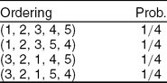
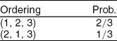
Comments

No Comments have been published for this article.

Article contents

Parties, Coalitions, and the Internal Organization of Legislatures

Abstract

Information

PREFERENCES: PARTIES AS GROUPS OF LIKE-MINDED LEGISLATORS

Issue Preferences

Preference Polarization

LEGISLATIVE DECISION MAKING

Majoritarian Legislature

A “Busy” Legislature

LEGISLATIVE BEHAVIOR

Policy-making Equilibrium

Organizational Equilibrium

Weaker Forms of Intraparty Preference Affinities

DISCUSSION

Theories of Congress Reconsidered: Conditional Party Government

Theories of Congress Reconsidered: Procedural Cartel Theory

Theories of Congress Reconsidered: Pivotal Politics Model

Empirical Implications

CONCLUSION

APPENDIX

Footnotes

References

REFERENCES

Comments

Save article to Kindle

Save article to Dropbox

Save article to Google Drive

Reply to: Submit a response

Your details

You have entered the maximum number of contributors

Conflicting interests