1 Introduction
As wind-driven water waves approach coastal structures, a handful of physical phenomena may arise owing to irregular sea bed topographies. For instance, these wind-generated waves may induce erosion or deposition at the sea bed. To increase the lifespan of coastal infrastructure, including bays, harbours and ports, researchers are turning their attention to investigating the interaction between surface waves and barriers, considering diverse sea bed profiles, to establish tranquility zones by reflecting or dissipating the maximum incident wave energy. To achieve these objectives, many kinds of breakwaters are implemented globally. In deep marine depths, conventional breakwaters such as rubble-mounded and concrete caissons are very practical, yet they are expensive to construct. Research suggests that water wave energy is predominantly localized near the free-sea surface; consequently, rigid floating and vertical breakwaters (optimal immersion) are recommended for effectively reflecting wave energy from the open sea. In real-life marine scenarios, the sea bed typically has an undulated profile, over which structures such as floating or vertically placed barriers are constructed to reflect incident wave energy from the open sea. In this context, numerous researchers have employed various experimental, theoretical, and numerical methods to study the scattering of surface water waves by single or multiple vertical barriers, under different assumptions regarding the sea bed profile. These efforts highlight the ongoing need for a comprehensive understanding of the effectiveness of breakwaters under realistic sea bed conditions. In this context, Ursell [Reference Ursell42] introduced the effect of a thin vertical plate on surface wave train in deep sea and derived expressions for the reflection and transmission characteristics with the aid of modified Bessel functions, whereas Evans [Reference Evans8] utilized the reduced velocity potential to obtain these characteristics and the expressions for first- and second-order forces and moments on the barrier. Losada et al. [Reference Losada, Losada and Roldan19] studied the effect of a thin vertical barrier for three different configurations on surface gravity waves using a matched eigenfunction expansion technique in conjunction with analytical an least-squares approach and further calculated the reflection and transmission characteristics. Instead of a flat bed, Mandal and Gayen [Reference Mandal and Gayen22] considered a partially immersed thin vertical barrier over small undulations at the sea bottom and utilized a simplified perturbation analysis to examine the scattering problem. Using the one-term Galerkin approximation technique, Mandal and Das [Reference Mandal and Das21] and Ray et al. [Reference Ray, De and Mandal30] observed the diffraction of monochromatic surface gravity waves by a vertical plate in deep water and over an infinite step bottom, respectively, to reveal the reflection and transmission characteristics. Further, Choudhary et al. [Reference Choudhary, Koley and Martha5] considered the thick vertical barrier over an arbitrary bottom topography and solved the problem using a coupled eigenfunction expansion and boundary element method. Manisha et al. [Reference Manisha, Kaligatla and Sahoo23] considered the barrier in the form of a floating bridge over an undulated bottom and solved the problem with the aid of modified mild-slope and eigenfunction expansion methods, and calculated the wave forces for reducing wave loads on a floating bridge. Additionally, porosity and flexibility of the vertical barrier were taken into account by Koley et al. [Reference Koley, Kaligatla and Sahoo16] and Kaligatla et al. [Reference Kaligatla, Koley and Sahoo13]. Both employed an integral equation approach to find various wave characteristics in both the cases of water of finite and infinite depths. Further, Koley and Sahoo [Reference Koley and Sahoo17] utilized a coupled boundary element and finite difference technique to analyse the interaction of obliquely incident surface gravity waves with a vertical flexible permeable submerged membrane wave barrier. In their latest endeavour, Goyal and Martha [Reference Goyal and Martha9] investigated a thick barrier interaction with surface waves over a nonuniform monotonically decreasing oscillatory bathymetry using the boundary element method in conjunction with the eigenfunction expansion technique and highlight that the bottom topography plays a vital role in altering the wave characteristics. Meylan and Stepanyants [Reference Meylan and Stepanyants25] studied a specific case of gravity-capillary wave transformation on bottom obstacles in the forms of a step, hump and trench, using the heuristic method.
To enhance the wave-reflecting performance of a single barrier, several researchers have investigated the scattering of water waves by dual vertical barriers, considering the presence or absence of various bottom topographies. In this context, Newman [Reference Newman28] studied the impact of thin dual vertical plates on surface waves with the aid of modified Bessel functions for deep water and obtained expressions for reflection and transmission characteristics, whereas the same problem was examined by McIver [Reference McIver24] for finite water depth using the eigenfunction expansion method. Further, using numerical approximation methods, Das et al. [Reference Das, Dolai and Mandal6] considered the one-term Galerkin approximation technique to investigate the diffraction of ocean currents in uniform depths of water by dual thin vertical barriers. A similar problem with nonidentical dual rigid thin vertical plates was considered by Roy et al. [Reference Roy, Basu and Mandal32] in infinitely deep water. Further, Gupta and Gayen [Reference Gupta and Gayen10] extended the problem of Roy et al. [Reference Roy, Basu and Mandal32] to porous dual vertical barriers and studied the influence of permeability using the multi-term Galerkin approximation technique. Utilizing the same Galerkin technique, Sarkar et al. [Reference Sarkar, Roy and De39] investigated the wave propagation over an asymmetric rectangular trench in the presence of dual partially immersed thin vertical barriers. Various researchers, among them Rezanejad et al. [Reference Rezanejad, Bhattacharjee and Soares31], Wang et al. [Reference Wang, Deng, Wang and Wang43] and Chanda and Bora [Reference Chanda and Bora3], also analysed the effect of dual vertical barriers under the influence of ocean currents by an eigenfunction expansion methodology in conjunction with some numerical techniques. Rezanejad et al. [Reference Rezanejad, Bhattacharjee and Soares31] analysed the efficiency of a double-chamber oscillating water column over a stepped bottom by utilizing both the eigenfunction expansion method and the boundary integral equation method. Wang et al. [Reference Wang, Deng, Wang and Wang43] solved the scattering problem by two thin surface piercing vertical plates over a stepped-type bottom profile using the eigenfunction expansion method in conjunction with the least-squares approach to derive the reflection coefficient, horizontal forces acting on the two barriers, and the free surface elevation. Chanda and Bora [Reference Chanda and Bora3] incorporated the permeability of sea bed over flat bed and analysed the ocean wave mitigating effect of dual thin vertically submerged barriers using eigenfunction expansion and the least-squares method. Further, Sarkar and De [Reference Sarkar and De37] studied the hydrodynamic performance of a pair of partially immersed barriers just above a thick, rigid bottom-standing barrier using Galerkin’s approximation technique. Later on, Sarkar et al. [Reference Sarkar, De and Gayen38] took into account the porosity of this pair of barriers, which are placed at different positions over a thick rectangular obstacle, utilizing the same approximation technique. Isaacson et al. [Reference Isaacson, Baldwin, Premasiri and Yang12] developed a physical model in support of their theoretical results which was carried out with the help of the eigenfunction method for the diffraction problem with dual thin vertical permeable barriers. Also, for the problem of dual vertical barriers, Neelamani and Vedagiri [Reference Neelamani and Vedagiri27] carried out an experimental investigation to obtain wave characteristics such as reflection, transmission, fluctuation and energy dissipation. Koley [Reference Koley15] deals with the interaction of obliquely incident gravity waves and a floating flexible porous plate over a variable bottom bed using a coupled eigenfunction expansion and boundary element method. Panduranga et al. [Reference Panduranga, Koley and Meylan29] studied surface wave interaction with submerged viscoelastic plates over an arbitrary bottom using a hybrid boundary element method in the frequency and time domain.
In addition to the aforementioned examination of the scattering of water waves caused by one or two thin vertical barriers, various researchers, such as Roy et al. [Reference Roy, De and Mandal33], Tran et al. [Reference Tran, Chang and Tsai40] and Nandi et al. [Reference Nandi, Sarkar, Hossain and De26], have recently considered multiple thin vertical barriers. Roy et al. [Reference Roy, De and Mandal33] and Nandi et al. [Reference Nandi, Sarkar, Hossain and De26] studied multiple thin vertical barrier problems using the multi-term Galerkin method for a uniform depth of water, whereas Tran et al. [Reference Tran, Chang and Tsai40] considered the bottom profile as undulating and discretized it into shelves, as a result of which they were able to utilize the matched eigenfunction method. Nandi et al. [Reference Nandi, Sarkar, Hossain and De26] investigated the interaction of surface waves after taking into account the flexibility and porosity of the multi-barriers. Also, a few researchers, such as Samanta et al. [Reference Samanta, Mondal and Banerjea34], Kaligatla et al. [Reference Kaligatla, Singh and Mandal14] and Tsai et al. [Reference Tsai, Behera and Hsu41], assumed more generalized forms of the breakwater such as an inclined or curved barrier. Samanta et al. [Reference Samanta, Mondal and Banerjea34] considered a circular arc-shaped barrier in a finite depth of water by employing the hyper-singular integral equation approach, while Kaligatla et al. [Reference Kaligatla, Singh and Mandal14] studied the interaction of a pi-type breakwater in deep ocean by using Galerkin’s approximation technique. Tsai et al. [Reference Tsai, Behera and Hsu41] investigated the interaction of multiple submerged semi-circular porous structures with surface waves using eigenfunction expansion and the multi-domain boundary element method.
In addition to the above literature, various researchers, such as Bai [Reference Bai1], Sannasiraj et al. [Reference Sannasiraj, Sundar and Sundaravadivelu35, Reference Sannasiraj, Sundaravadivelu and Sundar36] and Cho et al. [Reference Cho, Jeong and Woo4], handled the problems using a numerical technique, namely the finite element method (FEM). The scattering of obliquely incident ocean currents upon an infinite cylinder floating on the free surface was studied by Bai [Reference Bai1] using the FEM and calculated characteristics such as reflection and transmission, and also the horizontal force and moment on the floating cylinder. Sannasiraj et al. [Reference Sannasiraj, Sundar and Sundaravadivelu35, Reference Sannasiraj, Sundaravadivelu and Sundar36] performed a diffraction analysis due to floating structures on the flat sea bed and examined hydrodynamic roll, heave and sway responses using the FEM. In [Reference Sannasiraj, Sundaravadivelu and Sundar36] they studied pontoon-type floating breakwaters in beam waves, whereas in [Reference Sarkar and De37] they discussed the dynamics of multiple floating structures. Cho et al. [Reference Sarkar, De and Gayen38] developed a finite element model for abrupt depth changes and calculated reflection and transmission coefficients for the scattering of surface waves.
The above existing literature covers a variety of problems related to water wave scattering by single or dual barriers, utilizing a range of solution techniques for uniform and deep water depths, as well as for different bottom topographies. To the best of the authors’ knowledge, studies on the interaction of water waves with dual barriers over arbitrary bottom topographies are limited. It is evident that researchers encounter significant challenges when the sea bed profile is assumed to have arbitrary undulations, often necessitating the use of numerical or semi-analytical methods. It is worth noting that enhanced wave attenuation in harbours can be achieved by installing dual barriers, which dissipate wave energy more effectively than a single barrier, thereby enabling safer docking and cargo operations even over uneven sea bed profiles. Hence, in this paper, an effort is made to investigate the interaction of water waves with two vertical barriers over an arbitrary bottom topography. Two types of sea bed profiles are considered: a parabolic type and a rectangular type. The parabolic bottom profile is often used to model naturally occurring smooth sea bed slopes such as those found in coral reef systems (for example, the Great Barrier Reef, Australia, as mentioned in Beamam et al. [Reference Beaman, Webster and Wust2]) or offshore sandbars, where sediment deposition creates a gradual, curved bathymetry. This profile is particularly useful in studying wave shoaling and scattering over gently varying topographies, as demonstrated by Lin and Liu [Reference Lin and Liu18]. In contrast, the rectangular bottom profile approximates abrupt depth changes, such as those near submerged breakwaters (see Losada et al. [Reference Losada, Silva and Losada20] who model the interaction of regular waves with submerged structures) or artificial reefs (Xu et al. [Reference Xu, Tao, Wang, Qin, Fan, Xing, Wang, Wang and Zheng44] and Huang et al. [Reference Huang, Lowe, Ghisalberti and Hansen11]). Additionally, a sinusoidal bottom profile has been used for comparison purposes.
The general mathematical formulation of the present boundary value problem, concerning the interaction of surface waves with dual vertical barriers over arbitrary bottom profiles, is presented in Section 2. The numerical method of solution, namely the FEM, is detailed in Section 3. The energy identity is derived in Section 4. Section 5 provides the numerical results and discussion on the reflection coefficient, transmission coefficient, and nondimensional horizontal forces on both the front and rear barriers, as well as the influence of system parameters on these physical quantities. Section 6 presents the key conclusions.
2 Mathematical formulation
The mathematical modelling of the physical problem is analysed in a three- dimensional Cartesian coordinate system
 $(x,y,z)$
such that the positive direction of the y-axis is taken vertically downward and the
 $(x,z)$
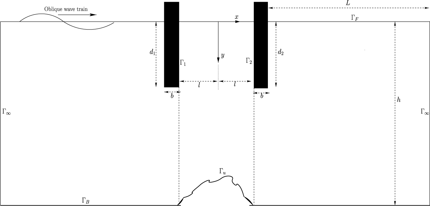
plane coincides with the undisturbed free surface of seawater. We consider the oblique incidence of the progressive wave train that makes an angle
 $\alpha $
with the positive x-axis to a pair of surface-piercing thick rigid vertical barriers in the presence of the bottom topography, which is arbitrary. Let
 $d_1$
and
 $d_2$
be drafts of the front barrier (FB) and rear barrier (RB) with positions
 $x=-l$
and l, respectively, and b be the thickness of both FB and RB. The widths of the barriers and the bottom topography are assumed to be infinitely long in the z-axis direction, so the edge effects are negligible. As the geometry of the breakwater does not vary in the z-direction, the characteristic behaviour remains uniform in the z-axis direction. Here, we look for a velocity potential that is periodic in the z-direction such that the z-part can be separated from the solution to make the study two-dimensional. Under linearized wave theory, we suppose the fluid under our consideration is inviscid, incompressible, and the motion is irrotational and harmonic in time with angular frequency
 $\omega $
. Therefore, the velocity potential can be written in the form
 ${\Phi (x,y,z,t)=\Re [\phi (x,y)e^{i(\mu z-\omega t)}]}$
, where
 $\Re $
denotes the real part and
 $\mu $
is the component of the wave number
 $k_0$
in the z-direction,
 $\mu =k_0 \sin \alpha $
. Here, the spatial velocity potential
 $\phi (x,y)$
is taken as the sum of the incident wave potential denoted by
 $\phi _{\mathrm {inc}}(x,y)$
and the scattered wave potential denoted by
 $\phi _{\mathrm {sc}}(x,y)$
such that
 $$ \begin{align*} \phi(x,y)=\phi_{\mathrm{inc}}(x,y) + \phi_{\mathrm{sc}}(x,y), \end{align*} $$
where
 $$ \begin{align*} \phi_{\mathrm{inc}}(x,y)=-\frac{Ag}{\omega}\frac{\cosh(k_0(y-h))}{\cosh(k_0h)}e^{i(k_0\cos\alpha) x}, \end{align*} $$
A is the incident wave amplitude, g is the acceleration due to gravity, h is the finite depth of water away from the arbitrary undulated profile and
 $k_0$
is the wave number of the incident wave, which is the positive real root of the dispersion equation
 ${\omega ^2 h/g =kh\tanh (kh)}$
.
The scattered velocity potential
 $\phi _{\mathrm {sc}}(x,y)$
satisfies the Helmholtz equation given by
 $$ \begin{align*} \frac{\partial^2 \phi_{\mathrm{sc}}}{\partial x^2}+\frac{\partial^2 \phi_{\mathrm{sc}}}{\partial y^2}-\mu^2\phi_{\mathrm{sc}}=0 \end{align*} $$
within the fluid domain
 $\Omega $
. Apart from the governing differential equation, the scattered potential must satisfy the following boundary conditions:
 $$ \begin{align*} &\frac{\partial\phi_{\mathrm{sc}}}{\partial y}+\frac{\omega^2}{g}\phi_{\mathrm{sc}}=0\quad \mathrm{on\,the\,free\,surface,}\\ &\frac{\partial\phi_{\mathrm{sc}}}{\partial y}=0\quad \mathrm{~on\ the\ flat\ bottom,}\\ &\frac{\partial\phi_{\mathrm{sc}}}{\partial n}=-\frac{\partial\phi_{\mathrm{inc}}}{\partial n} \quad \mathrm{on\, the \,barriers \,and\, arbitrary\, bottom,} \end{align*} $$
where n represents the unit outward normal on the barriers and the arbitrary bottom. Finally, we impose the following radiation boundary conditions on the scattered potential at infinity to make the solution unique:
 $$ \begin{align} \frac{\partial\phi_{\mathrm{sc}}}{\partial x} \pm (i k_0\cos\alpha)\, \phi_{\mathrm{sc}}=0\quad \mathrm{on\ infinite\ boundaries,\ that\ is}, x\to \mp \infty. \end{align} $$
But, we impose the radiation boundary conditions (2.1) at a finite distance from the barriers as the local disturbances decay sufficiently in a finite distance, say L, which is proven in Section 5. Thus, we have a well-posed boundary value problem, which is defined in a finite domain after truncating the infinite domain as shown in Figure 1, where
 $\Gamma _F$
,
 $(\Gamma _1,\Gamma _2)$
,
 $\Gamma _B$
,
 $\Gamma _u$
,
 $\Gamma _\infty $
are, respectively, the free surface, FB and RB boundary, flat bottom boundary, arbitrary undulation boundary, and radiation boundaries. Let us rewrite the final formulation after dropping the sc subscript from “
 $\phi _{\mathrm {sc}}$
”, before implementing the finite element method as follows:
 $$ \begin{align} &\frac{\partial^2 \phi}{\partial x^2}+\frac{\partial^2 \phi}{\partial y^2}-\mu^2\phi=0 \quad\mathrm{in}\; \Omega , \end{align} $$
 $$ \begin{align} &\frac{\partial\phi}{\partial n}+\frac{\omega^2}{g}\phi=0 \quad\mathrm{ on}\; \Gamma_F, \end{align} $$
 $$ \begin{align} &\frac{\partial\phi}{\partial n}=0 \quad \mathrm{on}\; \Gamma_B, \end{align} $$
 $$ \begin{align} &\frac{\partial\phi}{\partial n}=-\frac{\partial\phi_{\mathrm{inc}}}{\partial n} \quad \mathrm{on}\; \Gamma_S(=\Gamma_u\cup\Gamma_1\cup\Gamma_2), \end{align} $$
 $$ \begin{align} &\frac{\partial\phi}{\partial n} - (i k_0\cos\alpha)\, \phi=0 \quad \mathrm{on} \; \Gamma_\infty. \end{align} $$
We now aim to solve the boundary value problem (2.2)–(2.6) to determine the scattered potential
 $\phi $
.
Schematic of the problem.

3 Method of solution
We employ the finite element method to solve this problem of having arbitrary bottom topography between the surface-piercing barriers.
3.1 Finite element formulation
For the present study, we employ a two-dimensional FEM to solve the boundary value problem for the scattered velocity potential. There are commonly two ways, namely the variational method and the weighted residual method, to construct the integral formulation for the governing partial differential equation. As the approximated potential is substituted into the governing equation with the boundary conditions, a residual occurs at each node, which is forced to be equal to zero by employing the weighted residual method. The scattered velocity potential
 $\phi $
is approximated as a linear combination of the shape functions
 $N^{e}_{i}(x,y)$
and the nodal values
 $\phi ^{e}_{i}$
over each typical element e as
 $$ \begin{align} \hat{\phi^{e}}= \sum_{i=1}^{n_e}\phi^{e}_{i} N^{e}_{i}(x,y), \end{align} $$
where
 $\hat {\phi ^{e}}$
denotes the approximated scattered velocity potential and
 $n_e$
the number of nodes over an element.
On calculating the weighted residual of the governing differential equation (2.2) using the weight function,
 $w\equiv w(x,y)$
, over each element and forcing it to be equal to zero, we obtain
 $$ \begin{align} 0&=\int_{\Omega^{e}}-w \,\bigg(\frac{\partial^2 \hat{\phi^{e}}}{\partial x^2}+\frac{\partial^2 \hat{\phi^{e}}}{\partial y^2}-\mu^2\hat{\phi^{e}}\bigg)\,d\Omega^{e}, \nonumber \\ & \quad\Rightarrow 0=\int_{\Omega^e}\bigg(\frac{\partial w}{\partial x}\frac{\partial \hat{\phi^e}}{\partial x}+\frac{\partial w}{\partial y}\frac{\partial \hat{\phi^e}}{\partial y}+\mu^2 w \hat{\phi^e}\bigg)\,d\Omega^e-\int_{\Gamma^e}w\frac{\partial\hat{\phi^e}}{\partial n}\,d\Gamma^e , \end{align} $$
where
 $\Omega ^e$
and
 $\Gamma ^e$
respectively represent the domain and boundary of a typical element in which the corresponding integrations are taken. The second integral term (corresponding to the boundaries) may be written as
 $$ \begin{align} \int_{\Gamma^e}w\frac{\partial\hat{\phi^e}}{\partial n}\,d\Gamma^e=-\frac{w^2}{g}\int_{\Gamma_{F}^{e}}w\hat{\phi^e}\,d\Gamma_{F}^e+0+\int_{\Gamma_{\infty}^{e}} w (ik_0\cos\alpha)\hat{\phi^e}\,d\Gamma_{{\infty}^{e}}+Q^e , \end{align} $$
where
 $$ \begin{align*} Q^e=\int_{\Gamma_{S}^e}w\,\bigg(-\frac{\partial\phi_{\mathrm{inc}}}{\partial n}\bigg)\,d\Gamma_{S}^e. \end{align*} $$
The weight functions
 $w(x,y)$
are to be chosen as a set of linearly independent functions. In the Galerkin approach,
 $w=N_j \,(j=1,2,3,\ldots ,n_e)$
are taken as the choice of weight functions. Now, substituting expressions (3.1) and (3.3) into equation (3.2) and simplifying, we obtain
 $$ \begin{align*} \sum_{i=1}^{n_e}\phi_i^e & \bigg[\int_{\Omega^e}\bigg(\frac{\partial N_i^e}{\partial x}\frac{\partial N_j^e}{\partial x}+\frac{\partial N_i^e}{\partial y}\frac{\partial N_j^e}{\partial y}+\mu^2 N_i^e N_j^e\bigg)\, d\Omega^e+\frac{w^2}{g}\int_{\Gamma_{F}^{e}}N_i^e N_j^e \,d\Gamma_{F}^{e} \nonumber\\ & \quad -ik_0\cos\alpha\int_{\Gamma_{\infty}^{e}}N_i^e N_j^e\, d\Gamma_{\infty}^{e} \bigg]=\int_{\Gamma_{S}^e}N_j^e\bigg(-\frac{\partial\phi_{\mathrm{inc}}}{\partial n}\bigg)\, d\Gamma_{S}^e , \end{align*} $$
where
 $j=1,2,3,\ldots ,n_e,$
 $$ \begin{align} \Rightarrow \sum_{i=1}^{n_e}\phi_i^e & \bigg[\int_{\Omega^e}\bigg(\frac{\partial N_i^e}{\partial x}\frac{\partial N_j^e}{\partial x}+\frac{\partial N_i^e}{\partial y}\frac{\partial N_j^e}{\partial y}+\mu^2 N_i^e N_j^e\bigg)\, d\Omega^e+\frac{w^2}{g}\int_{\Gamma_{F}^{e}}N_i^e N_j^e \, d\Gamma_{F}^{e} \nonumber\\ & \quad -ik_0\cos\alpha\int_{\Gamma_{\infty}^{e}}N_i^e N_j^e \, d\Gamma_{\infty}^{e} \bigg]=-Q_j^e. \end{align} $$
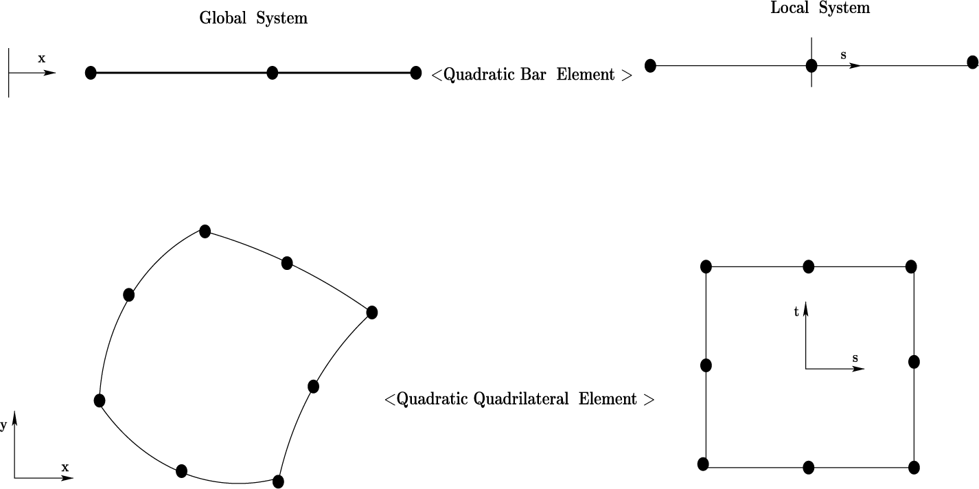
The computational domain of the problem is divided into finite elements by using two types of isoparametricFootnote 1 elements. The quadratic bar and quadratic quadrilateral elements correspond to the boundaries and the inner domain, respectively. The local and global coordinate systems for isoparametrization are given in Figure 2, and the shape functions for each node in any element in the local system are given below.
Quadratic bar and quadrilateral element.

The shape functions for the quadratic bar element are
 $$ \begin{align*} N_1^e=\frac{-s(1-s)}{2}, \quad N_2^e=(1-s)(1+s), \quad N_3^e=\frac{s(1+s)}{2}, \end{align*} $$
whereas the shape functions for quadratic quadrilateral elements are
 $$ \begin{align*} N_1^e & = -\tfrac{1}{4}(1-s)(1-t)(1+s+t),\\ N_2^e & =\tfrac{1}{2}(1-s^2)(1-t),\\ N_3^e & = -\tfrac{1}{4}(1+s)(1-t)(1-s+t), \\ N_4^e & =\tfrac{1}{2}(1+s)(1-t^2),\\ N_5^e & = -\tfrac{1}{4}(1+s)(1+t)(1-s-t), \\ N_6^e & =\tfrac{1}{2}(1-s^2)(1+t),\\ N_7^e & = -\tfrac{1}{4}(1-s)(1+t)(1+s-t), \\ N_8^e & =\tfrac{1}{2}(1-s^2)(1-t). \end{align*} $$
From equation (3.4), we can derive the element stiffness matrix
 $[k_{ij}^e]$
and the load vector
 ${Q_j^e}$
for the unknown nodal values
 ${\phi _i^e}$
for each element in the form as
 $$ \begin{align*} [k_{ij}^e]_{n_e\times n_e}\{\phi_i^e\}_{n_e\times 1}=\{Q_{j}^e\}_{n_e\times 1}, \end{align*} $$
where
 $$ \begin{align*} k_{ij}^e&=\int_{\Omega^e}\bigg(\frac{\partial N_i^e}{\partial x}\frac{\partial N_j^e}{\partial x}+\frac{\partial N_i^e}{\partial y}\frac{\partial N_j^e}{\partial y}+\mu^2 N_i^e N_j^e\bigg)d\Omega^e+\frac{w^2}{g}\int_{\Gamma_{F}^{e}}N_i^e N_j^e d\Gamma_{F}^{e}\\ & \quad -ik_0\cos\alpha\int_{\Gamma_{\infty}^{e}}N_i^e N_j^e d\Gamma_{\infty}^{e} , \end{align*} $$
and
 $$ \begin{align*} Q_j^e=\int_{\Gamma_{S}^e}N_j^e\bigg(-\frac{\partial\phi_{\mathrm{inc}}}{\partial n}\bigg)d\Gamma_{S}^e , \end{align*} $$
which is further assembled to get a global stiffness matrix
 $[K_{ij}]$
and global load vector
 $\{Q_j\}$
over the elements and has to solve for unknown global nodal values. Once the scattered potential is determined, the behaviour of the reflected waves (RWs) and transmitted waves (TWs) can be investigated. The reflection and transmission coefficients of monochromatic surface waves are calculated by using the following relations:
 $$ \begin{align*} \vert R \vert &= \frac{\omega}{A g}\frac{\cosh k_0h}{\cosh k_0(y_0-h)}\vert \phi(-L,y_0)\vert , \\ \vert T \vert &= \frac{\omega}{A g}\frac{\cosh k_0h}{\cosh k_0(y_0-h)}\bigg\vert \frac{A g}{\omega}\frac{\cosh k_0(y_0-h)}{\cosh k_0h}-e^{-i(k_0\cos{\alpha})x} \phi(L,y_0)\bigg\vert , \end{align*} $$
where
 $ y_0\in [0,h]$
is any point. The horizontal force on the FB and RB is derived from Bernoulli’s equation for the unit amplitude of the incident wave (IW). In nondimensional form, the horizontal force per unit width on the FB is
 ${\vert F_f\vert }/{\rho g h A}$
and on the RB is
 ${\vert F_r\vert }/{\rho g h A}$
, given by the integrals
 $$ \begin{align*} \frac{\vert F_f\vert}{\rho g h A}&=\frac{\omega}{gh}\bigg\vert\!\int_{0}^{d_1}(\phi(-b-l,y)-\phi(-l,y))dy\bigg\vert ,\\ \frac{\vert F_r\vert}{\rho g h A}&=\frac{\omega}{gh}\bigg\vert\!\int_{0}^{d_2}(\phi(b+l,y)-\phi(l,y))dy\bigg\vert , \end{align*} $$
respectively, which are further solved numerically using Simpson’s 1/3 rule.
4 Energy identity relation
We use Green’s identity as given by
 $$ \begin{align} \int_{\Gamma}\bigg(\phi\frac{\partial \phi^{*}}{\partial n}-\phi^{*}\frac{\partial \phi}{\partial n}\bigg)d\Gamma=0 , \end{align} $$
where
 $\phi ^{*}(x,y)$
is conjugate of the complex potential
 $\phi (x,y)$
and
 ${\partial }/{\partial n}$
is the normal partial derivative in an outward direction to the boundary
 $\Gamma $
which is the boundary of the fluid region
 $\Omega $
.
The contribution due to free surface
 $\Gamma _F$
to the integral (4.1) is zero, as
 $$ \begin{align*} \int_{\Gamma_{F}}\bigg[\phi \bigg\{-\frac{\omega^2}{g}\phi^{*}\bigg\}-\phi^{*} \bigg\{-\frac{\omega^2}{g}\phi \bigg\}\bigg]\,dx=0. \end{align*} $$
The contribution due to the bottom (undulated and flat type),
 $\Gamma _{u}\cup \Gamma _{B}$
and both the barriers (FB and RB),
 $\Gamma _{1}\cup \Gamma _{2}$
to the integral (4.1) is also zero, since
 ${{\partial {\phi }}/{\partial {n}}={\partial {\phi ^{*}}}/{\partial {n}}=0}$
on the bottom and as well as on both the barriers.
The contribution from the left radiation boundary is
 $$ \begin{align*} \int_{0}^{h}\bigg(\phi\frac{\partial \phi^{*}}{\partial x}-\phi^{*}\frac{\partial \phi}{\partial x}\bigg)\,dy=\frac{A^2 g^2}{\omega^2}\frac{ik_0{\cos{\alpha}}(|R|^2-1)}{2k_0\cosh^2k_{0}h}[2k_0 h+\sinh2k_0 h]. \end{align*} $$
The contribution from the right radiation boundary is
 $$ \begin{align*} \int_{h}^{0}\bigg(\phi\frac{\partial \phi^{*}}{\partial x}-\phi^{*}\frac{\partial \phi}{\partial x}\bigg)\,dy=\frac{A^2 g^2}{\omega^2}\frac{ik_0{\cos{\alpha}}|T|^2}{2k_0\cosh^2k_{0}h}[2k_0 h+\sinh2k_0 h]. \end{align*} $$
On adding all the above contributions to the integral (4.1), we get the energy identity as given by
 $$ \begin{align*} \vert R \vert^{2} + \vert T \vert^{2}=1. \end{align*} $$
5 Numerical results and discussion
Due to the applicability and relevance of arbitrary bottom topographies, specifically parabolic and rectangular forms, as described in the last paragraph of the introduction section, we consider two profiles in this study: parabolic hump (type I) and rectangular hump (type II). The type I profile is given by
 $$ \begin{align*} x(s)=s,\quad y(s)=\frac{c_0}{l^2}s^2+(-c_0+h)\quad \mathrm{for } -l\leq s\leq l. \end{align*} $$
The type II profile is given by
 $$ \begin{align*} x(s)=-l,\quad y(s)=s\quad \mathrm{for }\ h-c_0\leq s\leq h, \end{align*} $$
 $$ \begin{align*} x(s)=s,\quad y(s)=h-c_0 \quad \mathrm{for } -l < s < l, \end{align*} $$
 $$ \begin{align*} x(s)=l,\quad y(s)=s \quad \mathrm{for }\ h-c_0\leq s\leq h. \end{align*} $$
For comparison purposes, we also consider a third profile, the sinusoidal (type III) profile, given by
 $$ \begin{align} x(s)=s,\quad y(s)=h+c_0\sin{\lambda s} \quad \mathrm{for } -l\leq s\leq l;~~ l=M\pi/\lambda, \end{align} $$
where
 $\lambda $
is the wave number of the sinusoidal profile, M is a positive integer and
 $c_0$
is the height of the undulation.
In all configurations, the depth of the fluid domain on either side of the hump is assumed to be equal. The nondimensionalization of the physical parameters is carried out using the finite flat depth h of the fluid domain, as follows:
 $d_1/h$
,
 $d_2/h$
,
 $d/h(=d_1/h=d_2/h)$
,
 $b/h$
,
 $l/h$
,
 $L/h$
,
 $c_0/h$
,
 $k_0h$
,
 $\omega ^2h/g$
. Also, the nondimensional value of
 $c_0/h$
is taken to be zero to represent a flat bottom profile.
5.1 Convergence criteria
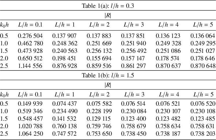
As previously emphasized, while solving the problem using the FEM, the radiation boundaries are placed at a finite distance, since the local disturbances caused by the barriers and the undulated bottom topography decay sufficiently within that range. The analysis of the data in Table 1 shows that a distance of four times the depth of the water is sufficient to keep the radiation boundaries for sufficient accuracy in the results
 $|R|$
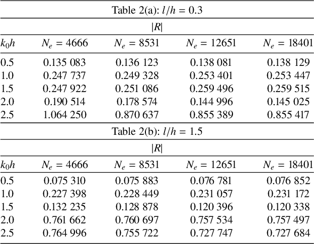
, and the same was stated by Bai [Reference Bai1]. The discretization of the computational domain is made using two types of elements, namely, quadratic quadrilateral elements within the domain and quadratic bar elements at the boundaries. The mesh element size is progressively refined to the next higher level, and its effect on the convergence of the finite element solution has been analysed in Table 2. The total number of elements in the computational domain, which is represented by
 $N_e$
, is increased as
 $4666, 8531, 12\,651$
and
 $18\,401$
, corresponding to
 $314, 474, 604$
and
 $750$
elements on the boundaries, respectively. The element’s shape is parsimoniously kept square by keeping the aspect ratio near to unity. This table demonstrates that for particular parameters, four-decimal-place accuracy in
 $|R|$
may be achieved in the present numerical results with
 $N_e=12\,651$
for all nondimensionalized wave number
 $k_0h$
values.
Effect of the distance
 $L/h$
of the radiation boundary conditions from the barriers on the finite element solutions through
 $|R|$
(
 $c_0/h=0.2, d_1/h=d_2/h=0.2, b/h=0.1, \alpha =0$
) for type I profile.

Convergence of number of elements
 $N_e$
through
 $|R|$
(
 $c_0/h=0.2, d_1/h=d_2/h=0.2, b/h=0.1, L/h=4, \alpha =0$
) for type I profile.

5.2 Validation
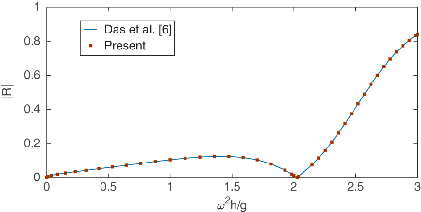
The numerical model developed here is initially used to calculate the reflection coefficient of scattering of normal incidence surface waves for a particular case where there is no undulation at the bottom (
 $c_0/h=0$
) and identical lengths of FB and RB (
 $d_1/h=d_2/h=0.2$
) and the positions at
 $l/h=0.3$
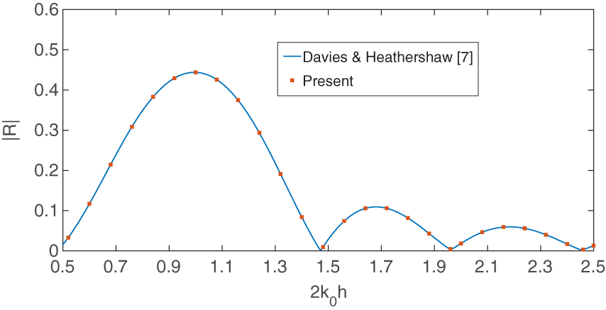
in order to validate the current numerical results. The reflection coefficient calculated from the present numerical model is compared with those predicted by Das et al. [Reference Das, Dolai and Mandal6] as shown in Figure 3, where good agreement is observed, and this validates the present results. In the absence of both barriers, with only the bottom profile in the form of a sinusoidal hump as assumed by Davies and Heathershaw [Reference Davies and Heathershaw7], a validation case is obtained by selecting the parameters
 $d_1/h=d_2/h=0, c_0/h=0.32, \lambda h=1$
and
 $M=2$
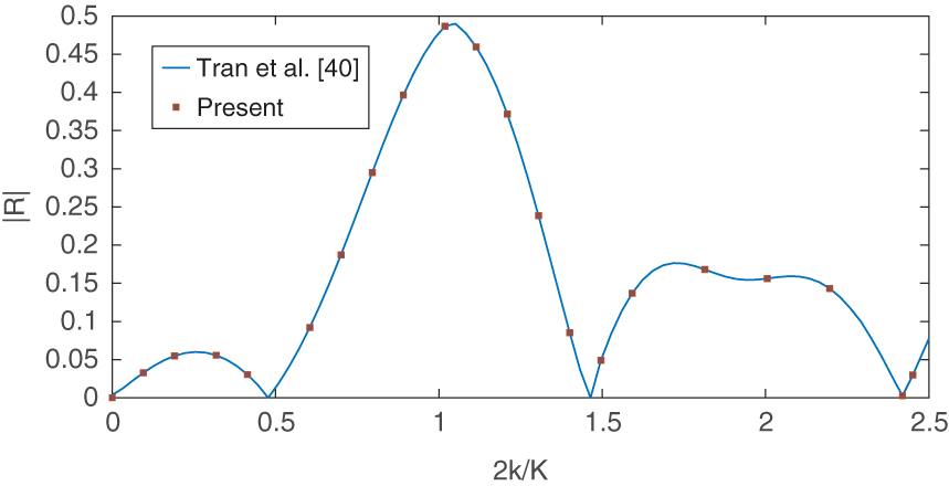
. The comparison, presented in Figure 4, shows good agreement. Another comparison is made with the results of Tran et al. [Reference Tran, Chang and Tsai40], who considered both vertical barriers and a sinusoidal bottom topography. This particular case can be reproduced in the present study by setting the barrier drafts to
 $ d_1/h = d_2/h = 0.2 $
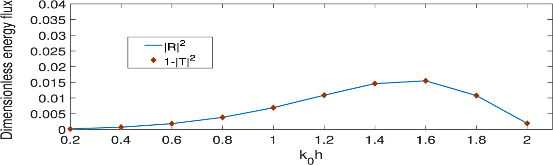
and selecting the sinusoidal profile as the arbitrary bottom topography. The comparison is shown in Figure 5, where excellent agreement is observed in the reflection coefficients. Furthermore, the energy identity relation
 $ |R|^2 + |T|^2 = 1 $
holds, serving as a numerical check for the computed results, as demonstrated in Figure 6. For Figures 3 and 6, the distance between the thin vertical identical barriers is
 $0.6h$
.
Comparison between the present and Das et al. [Reference Das, Dolai and Mandal6] results for dual barriers in the absence of undulation.

Comparison between the present and Davies and Heathershaw [Reference Davies and Heathershaw7] results for the sinusoidal undulated profile in the absence of barriers.

Comparison between the present results and Tran et al. [Reference Tran, Chang and Tsai40] for dual identical barriers over a sinusoidal profile.

Verification of energy identity for scattering by two thin identical barriers
 $d/h=0.2$
,
 $c_0/h=0.1$
over type I profile.

5.3 Variation of the reflection and transmission coefficients with various parameters
To examine the effect of the gap between barriers over the type I profile for normally incident waves,
 $\vert R \vert $
and
 $\vert T \vert $
are plotted against
 $k_0h$
in Figures 7 and 8, respectively, for identical barriers for different gap lengths
 $l/h$
, while
 $\vert R \vert $
and
 $\vert T \vert $
are plotted against
 $k_0h$
in Figures 9 and 10, respectively, for nonidentical barriers for different gap lengths
 $l/h$
. In Figures 7–10, the barriers are assumed to be thin. For the case of two identical barriers when
 $d/h=0.2$
, the zeros on the curve of
 $\vert R \vert $
against
 $k_0h$
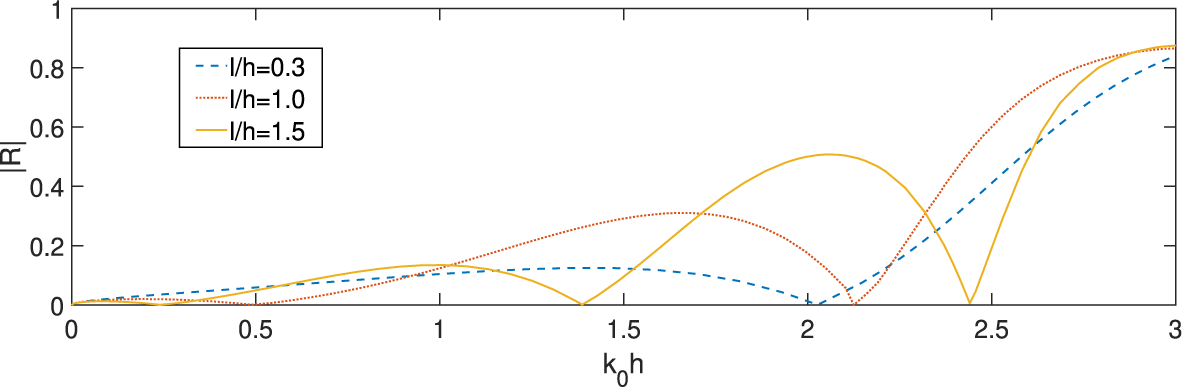
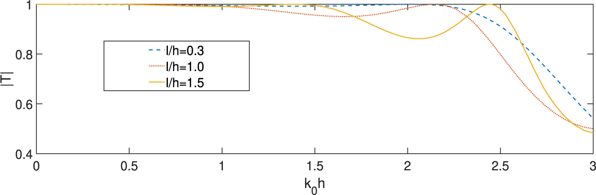
exist, and the number of zeros increases as the gap between the barriers increases as shown in Figure 7. This may happen due to the destructive and/or constructive interference between RW, IW and TW between the barriers. Corresponding to the zeros of the reflection coefficient, the transmission coefficient
 $\vert T \vert $
is unity, as shown in Figure 8. These zeros in the reflection curve should be avoided for the protection of coastal structures. It is also observed that as the gap
 $l/h$
between the barriers increases,
 $|T|$
converges to unity for lower to higher wave numbers, and then decreases, as shown in Figure 8. When the depths of submergence of the barriers are different (taking
 $d_1/h=0.18$
,
 $d_2/h=0.2$
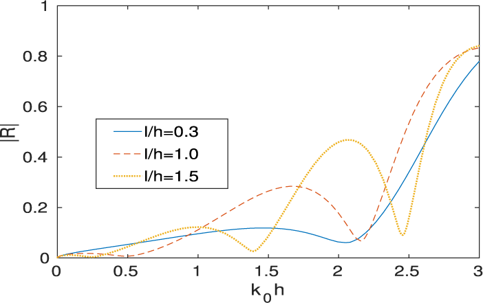
), Figure 9 shows the nonexistence of the zeros on the reflection curves. However, the minima and maxima still appear on the reflection curves, and the number of maxima and minima increases as the gap between the barriers increases. This may happen due to the mutual interaction between RW, IW, and TW. The behaviour of
 $\vert T \vert $
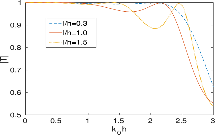
in Figure 10 is the same as in Figure 8.
 $|R|$
against
 $k_0h$
for
 $d_1/h=d_2/h=0.2$
,
 $c_0/h=0.1,\alpha =0$
for different positions
 $l/h$
of identical barriers.

 $|T|$
against
 $k_0h$
for
 $d_1/h=d_2/h=0.2$
,
 $ c_0/h=0.1, \alpha =0$
for different positions
 $l/h$
of identical barriers.

 $|R|$
against
 $k_0h$
for
 $d_1/h=0.18,_2/h=0.2$
,
 $ c_0/h=0.1, \alpha =0$
for different positions
 $l/h$
of nonidentical barriers.

 $|T|$
against
 $k_0h$
for
 $d_1/h=0.18,d_2/h=0.2$
,
 $ c_0/h=0.1, \alpha =0$
for different positions
 $l/h$
of nonidentical barriers.

As the reflection and transmission coefficients satisfy the energy conservation identity, the behaviour of the transmission coefficient can be inferred from the reflection coefficient curves. Therefore, the transmission coefficient curves are omitted from the subsequent results. For the rectangular hump profile in the range
 $[-l/h, l/h]=[-1.5,1.5]$
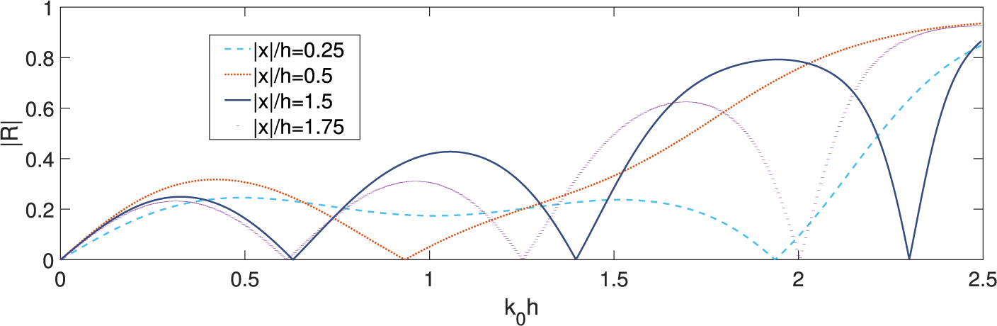
, Figure 11 shows
 $\vert R \vert $
against
 $k_0h$
for different
 $x/h$
-positions (
 $x/h=0.25,0.5,1.5,1.75$
) where the barrier can be placed. Here,
 $x/h=\pm 1.5$
represents, respectively, the exact right and left edge of the hump. From the figure, it is clear that barriers are more effective at the edges of the hump in reflecting incident waves, as the overall behaviour of
 $\vert R \vert $
appears consistent and the reflection coefficient increases when the barrier is positioned closer to the edges of the hump. It is also possible that, for different bottom undulation profiles, various positions may prove more effective in reflecting incident wave energy. Therefore, in the subsequent analysis, the barriers are positioned at the edges of the bottom topography.
 $|R|$
against
 $k_0h$
for
 $d_1/h=d_2/h=0.2,b/h=0.1,l/h=1.5,c_0/h=0.3,\alpha =0$
for different positions of the barriers over type II hump.

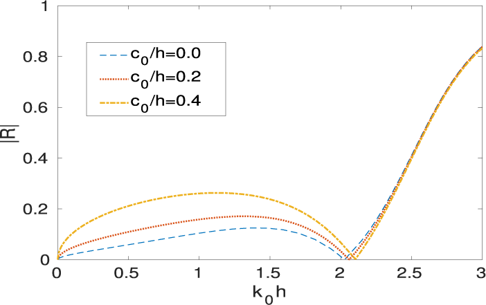
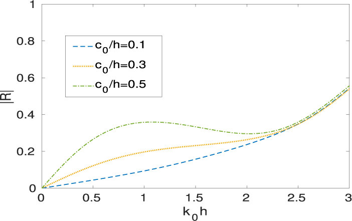
Now Figures 12 and 13 respectively show the effect of the height
 $c_0/h$
of the parabolic and rectangular hump on
 $\vert R\vert $
. In Figure 12, for identical barriers, the value of
 $\vert R\vert $
increases as
 $c_0/h$
increases for the wave numbers
 $0<k_0h<2$
. Meanwhile, the effect on the reflection coefficient is negligible for IWs with larger wave numbers
 $k_0h>2.2$
. The possible reason may be that the IWs with larger wave numbers are confined near the free surface. In Figure 13, for nonidentical barriers, it is again observed that
 $\vert R\vert $
increases as
 $c_0/h$
increases for smaller wave numbers while
 $\vert R\vert $
is negligibly affected due to larger wave number waves.
 $|R|$
against
 $k_0h$
for identical barriers
 $d_1/h = d_2/h=0.2, l/h=0.3, b/h=0.001, \alpha =0$
for different heights of type I hump.

 $|R|$
against
 $k_0h$
for nonidentical barriers
 $d_1/h$
=
 $0.1, d_2/h=0.2, b/h=0.001,l/h=0.5$
,
 $ \alpha =0$
for different heights of type II hump.

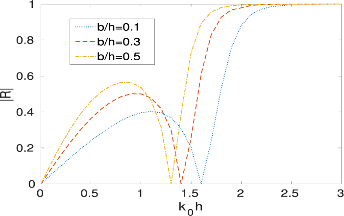
For three different barrier thicknesses
 $b/h$
,
 $\vert R\vert $
is presented against
 $k_0h$
in Figure 14. It is apparent that as
 $b/h$
increases,
 $\vert R\vert $
increases as well. This may be caused by the fact that IW and RW interact with each other between FB and RB. Additionally, a phase shift in
 $\vert R\vert $
has been observed, which may also be caused by the mutual interaction of waves with different wave numbers produced over the parabolic hump profile.
 $|R|$
against
 $k_0h$
for
 $d_1/h=d_2/h=0.3$
,
 $c_0/h=0.3, l/h=0.3, \alpha =0$
for different thickness of the barriers over type I hump.

In Figure 15,
 $\vert R\vert $
is shown against
 $k_0h$
for three different identical drafts
 $d/h$
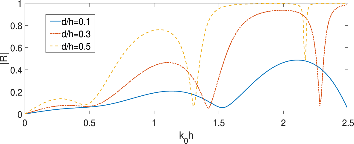
of the barriers over the parabolic hump profile. Here, the heights of local maxima on the
 $|R|$
curve increase by increasing the drafts
 $d/h$
of the barriers. This may be caused by the mutual interaction between RW, IW and TW between the barriers. Also, significant phase shifts in the oscillatory pattern of
 $\vert R\vert $
are observed as the length of barriers increases. This phase shift may happen due to the mutual interaction of waves with different wave numbers produced over the parabolic hump profile, as mentioned in Figure 14.
 $|R|$
against
 $k_0h$
for
 $b/h=0.1, c_0/h=0.2, l/h=1.5$
,
 $\alpha =0$
for different drafts of the barriers over type I hump.

In a similar pattern, the heights of the local maxima on the
 $\vert R\vert $
curve go high by increasing the drafts
 $d/h$
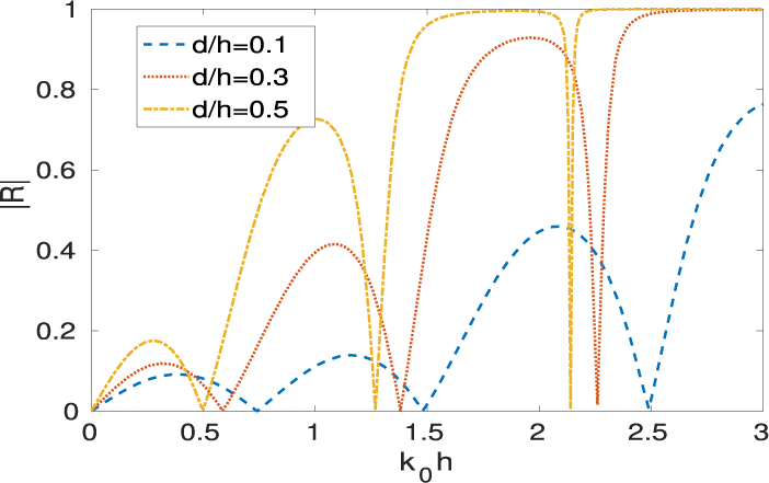
of the barriers placed over the sinusoidal hump bottom as shown in Figure 16. It is observed that
 $\vert R\vert $
increases as the length of the barrier increases for
 $d/h=0.1,0.3,0.5.$
But the zeros that exist on the curve of
 $\vert R\vert $
against
 $k_0h$
in Figure 15 for the parabolic hump topography are absent from the scenario for the sinusoidal hump topography in Figure 16 because the barrier spacing may be tuned to the incident wavelength, causing successive reflections between them to undergo destructive interference.
 $|R|$
against
 $k_0h$
for
 $b/h=0.1, c_0/h=0.2$
,
 $l/h=1.5, \alpha =0$
for different draft of the barriers over type III hump.

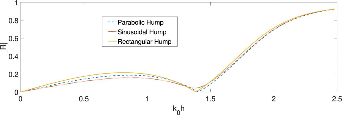
Finally, we compare the three bottom profiles in Figure 17 for
 $\vert R\vert $
against
 $k_0h$
for their reliability with dual vertical barriers. The rectangular hump profile is better than the other two profiles for given values of the parameters.
 $|R|$
against
 $k_0h$
for
 $d/h=0.2,b/h=0.1, c_0/h=0.2, l/h=1.5$
over different bottom topographies.

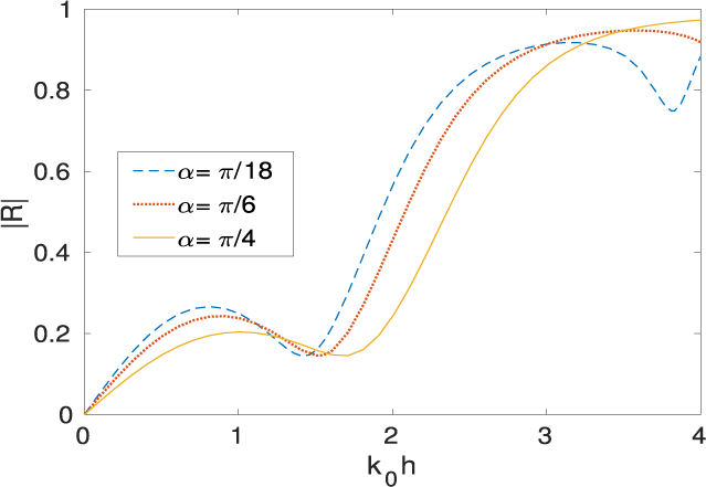
The effect of the angle of incidence
 $\alpha $
on
 $\vert R\vert $
against
 $k_0h$
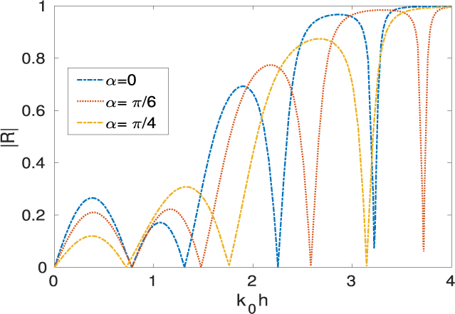
is shown for barriers over the parabolic and rectangular hump bottom profile in Figures 18 and 19, respectively. As the angle of incident
 $\alpha $
increases from 0 to
 $\pi /6$
and
 $\pi /4$
, the first local maxima on the
 $\vert R\vert $
curve decreases. After that, the local maxima on the
 $\vert R\vert $
curve increase as the value of
 $\alpha $
increases, as shown in Figure 18. This may happen due to the destructive and/or constructive interference between RW, IW, and TW between the barriers. The local maxima in
 $\vert R\vert $
shift toward the right as
 $\alpha $
increases. This phase shift in
 $\vert R\vert $
may occur for the same reason as mentioned in Figure 14. In Figure 19, the local maxima on the
 $\vert R\vert $
curve decrease as
 $\alpha $
increases from
 $\pi /18$
to
 $\pi /6$
and
 $\pi /4$
. Here, it is to be noticed that the use of nonidentical barriers prevents the occurrence of the phenomenon of zero reflection.
 $|R|$
against
 $k_0h$
for
 $d_1/h=d_2/h=0.2, b/h=0.1, c_0/h=0.5$
,
 $l/h=1.5$
for different angle of incidence over type I hump.

 $|R|$
against
 $k_0h$
for
 $d_1/h=0.1,d_2/h=0.2, b/h=0.1, c_0/h=0.3, l/h=0.5$
for different angle of incidence over type II hump.

5.4 Force on the barriers
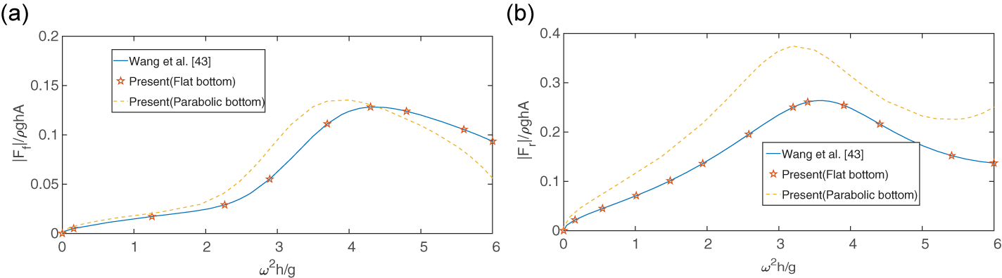
Figures 20(a) and 20(b) respectively show the nondimensionalized horizontal force on FB and RB variation with respect to
 $\omega ^2h/g$
for
 $d_1/h=0.1$
,
 $d_2/h=0.2$
,
 $b/h=0$
,
 $\alpha =\pi /6$
,
 $l/h=0.25$
for the flat bottom
 $c_0/h=0$
and parabolic bottom
 $c_0/h=0.3$
. The peak in both of these plots refers to the resonant motion due to the mutual interaction of the RW, IW and TW, between the vertical barriers. Here, the good agreement of these force profiles with those of Wang et al. [Reference Wang, Deng, Wang and Wang43], for the same parameter values, further confirms the correctness of the present method.
Nondimensional horizontal force against
 $\omega ^2h/g$
(a) on FB, and (b) on RB.

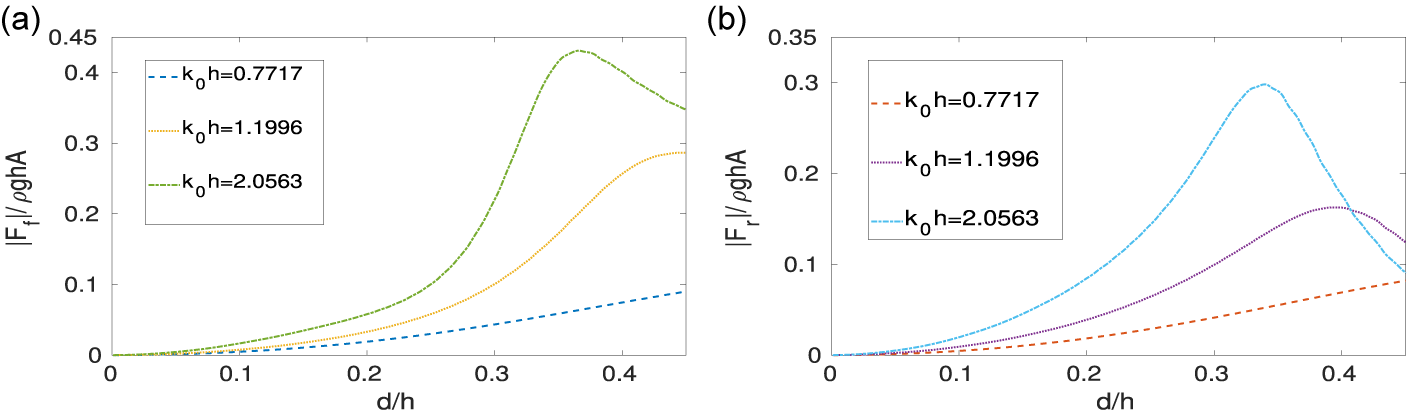
Figures 21(a) and 21(b) respectively show the variation of the nondimensional horizontal force on FB and RB with respect to drafts of the barriers
 $d/h$
over the rectangular hump bottom topography for three different wave numbers
 ${k_0h=0.7717,1.1996,2.0563}$
. It is observed that, as the wave number increases, the peaks of the horizontal force curves for both FB and RB increase. This is possible because IW energy with higher values of wave numbers is mainly confined near the free sea surface. Furthermore, it is apparent that the force acting on FB is greater than the force acting on RB.
Nondimensional horizontal force against
 $d/h$
for
 $c_0/h=0.5, b/h=0,l/h=0.75$
for three different wave numbers over type II hump (a) on FB, and (b) on RB.

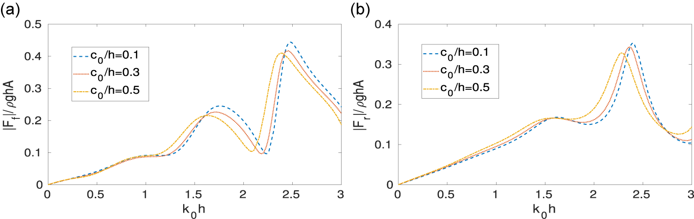
Figures 22(a) and 22(b) respectively show the variation of the nondimensional horizontal force against
 $k_0h$
for three different values of the heights of the parabolic hump on FB and RB. The value of the horizontal force does not change significantly for the wave numbers
 $0<k_0h<1.2$
and
 $0<k_0h<1.7$
on FB and RB respectively, but as the value of the wave numbers gets relatively larger, both the force profiles fluctuate. The diffraction force on FB is greater than that on RB. Both the figures show that local maxima in the force on FB and RB decrease as the height of the parabolic hump increases.
Nondimensional horizontal force against
 $k_0h$
for
 $d_1/h=d_2/h=0.2, b/h=0.1,\alpha =0, l/h=1.5$
for different heights of type I hump (a) on FB, and (b) on RB.

6 Conclusion
The current study examines the scattering of obliquely incident surface waves by two vertical barriers over an arbitrary bottom topography. The finite domain for this propagation problem is obtained by truncating the infinite domain at a finite distance. The resulting physical problem for two vertical barriers over an arbitrary bottom topography is then solved using the finite element technique. The computational domain of the problem is meshed by using two types of elements, namely, quadratic quadrilateral elements within the domain and quadratic bar elements at the boundaries. The physical quantities, specifically the reflection and transmission coefficients and the nondimensional horizontal force on the barriers, are numerically calculated. A convergence study for the total number of elements
 $N_e$
in the computational domain is conducted. Furthermore, the energy identity relation, derived from Green’s identity, is established and verified using the obtained numerical results. Numerical results are obtained for two specific cases of arbitrary bottom topography: the parabolic hump and the rectangular hump. Additionally, a comparison is made between these two bottom profiles and a sinusoidal hump. In the following, we have highlighted a few noteworthy observations.
-
• Numerical verification shows that placing the radiation boundary conditions at a distance equal to four times the water depth from the vertical barriers is sufficient, as local disturbances decay adequately within this range.
-
• Simplified formulas are derived to calculate the reflection and transmission coefficients with the aid of the velocity potential at the truncated boundaries.
-
• The zeros on the reflection curves exist for identical lengths of the barriers, and the number of zeros increases as the gap between them increases. Therefore, identical barrier lengths can be avoided in coastal protection.
-
• The local maxima on the transmission curve coalesce and approach unity as the gap between the barriers increases.
-
• For the dual vertical barriers over the sinusoidal hump profile, zeros on the reflection curves do not occur, as the barrier spacing may be tuned to the incident wavelength, causing successive reflections between the barriers to undergo destructive interference.
-
• It is observed that barriers placed at the edges of the rectangular hump profile are more effective at reflecting incident wave energy.
-
• It is observed that the reflection coefficient increases with the height of the bottom topography for smaller wave numbers, whereas the effect becomes negligible for larger wave numbers. This indicates that, for larger wave numbers, the water depth across the region can be considered sufficiently deep.
-
• The peak value of the reflection coefficient is proportional to the relative drafts and thickness of the barriers.
-
• In the case of dual barriers over a parabolic hump, as the angle of incidence increases, the first local maximum on the
 $|R|$
curve decreases, after which the local maxima begin to increase. In contrast, for the rectangular hump, the local maxima on the
$|R|$
curve continue to decrease with increasing angle of incidence.
-
• Under a specific set of parameter values, the rectangular bottom profile is found to reflect the maximum incident wave energy more effectively than the other two profiles.
-
• The impact of the hump’s height and the barriers’ drafts on the nondimensional horizontal force acting on both FB and RB is examined numerically. It is observed that the FB experiences a greater force than the RB. Therefore, the FB should be more structurally reinforced than the RB.


The present finite-element-based solution technique effectively models wave interaction with idealized sea bed profiles, including rectangular, parabolic and sinusoidal bottom geometries. However, the approach has certain limitations: it is based on linear wave theory and two-dimensional assumptions, thereby neglecting strong nonlinear effects and viscous dissipation. Additionally, the chosen sea bed profiles are simplified representations of natural bathymetry, and structural flexibility or porosity effects are not considered. Future work can extend the model to nonlinear and three-dimensional frameworks, incorporate dynamic sea bed evolution, and apply it to realistic field-measured bathymetries.
These concluding observations may assist engineers in designing effective breakwaters for coastal protection. Furthermore, this analysis could prove valuable in addressing similar problems encountered in applied mathematics and engineering.
Acknowledgement
S.C. Martha acknowledges the Anusandhan National Research Foundation (ANRF), Department of Science and Technology (DST), Government of India for the CRG grant (no. CRG/2023/008080).