1 Introduction
An important part of the study of the nonlinear regime of transition in wall flows is dedicated to the interaction of two or three Tollmien–Schlichting (TS) waves. Such studies established three routes for transition, namely,
 $K$
-type and
 $N$
-type (sometimes called
 $H$
-type or
 $C$
-type) transition and the oblique transition. In
 $K$
-type, a two-dimensional TS wave promotes the resonant growth of oblique waves with the frequency of the two-dimensional, fundamental wave (Klebanoff, Tidstrom & Sargent Reference Klebanoff, Tidstrom and Sargent1962). In
 $N$
-type, the nonlinear resonance promotes the growth of subharmonic oblique waves (Nishioka, Iida & Ichikawa Reference Nishioka, Iida and Ichikawa1975; Herbert Reference Herbert1983; Kachanov & Levchenko Reference Kachanov and Levchenko1984; Herbert Reference Herbert1988; Kachanov Reference Kachanov1994). These scenarios lead respectively to aligned and staggered patterns of
 $\unicode[STIX]{x1D6EC}$
-vortices. Oblique transition involves the development of a pair of oblique and opposite TS waves (Schmid & Henningson Reference Schmid and Henningson1992; Fasel, Thumm & Bestek Reference Fasel, Thumm, Bestek, Kral and Zang1993), and transition is preceded by the formation of streamwise vortices and longitudinal streaks.
In a natural environment, transition involves not only two or three interacting waves, but rather, a large number of two- and three-dimensional waves. Natural transition has the ingredients for all the classical nonlinear routes and perhaps much more. Wavepackets generated by pulse excitations contain a large number of interacting waves and have been shown to mimic natural transition to a large extent (Arnal & Juillen Reference Arnal and Juillen1977; Shaikh Reference Shaikh1997; Matsubara, Takaichi & Kenchi Reference Matsubara, Takaichi, Kenchi, Schlatter and Henningson2010). In view of this, the evolution of wavepackets has been studied in some detail. Gaster (Reference Gaster1975), Gaster & Grant (Reference Gaster and Grant1975) investigated the linear regime. Cohen, Breuer & Haritonidis (Reference Cohen, Breuer and Haritonidis1991) attributed the nonlinear regime of the packets to subharmonic instability, which was confirmed by Medeiros & Gaster (Reference Medeiros and Gaster1999a
,Reference Medeiros and Gaster
b
), Yeo et al. (Reference Yeo, Zhao, Wang and Ng2010). Wavepackets have also been studied in high-speed regimes (Sivasubramanian & Fasel Reference Sivasubramanian and Fasel2014), where
 $N$
-type,
 $K$
-type and oblique transition have been suggested. Simpler modulated models have also been investigated, an example being a wavetrain emanating from a point source, where only spanwise modulation is considered. This was studied by Mack (Reference Mack and Kozlov1985), Seifert (Reference Seifert1990), Seifert & Wygnanski (Reference Seifert and Wygnanski1991, Reference Seifert and Wygnanski1993), Wiegand et al. (Reference Wiegand, Bestek, Wagner and Fasel1995) in the linear regime. Stemmer, Kloker & Wagner (Reference Stemmer, Kloker and Wagner1998), Stemmer (Reference Stemmer2001) attributed to oblique transition the nonlinear regime of such a wave system in an adverse pressure gradient boundary layer. For a similar wave system in a flat plate boundary layer, Medeiros (Reference Medeiros2004b
) observed
 $K$
-type transition. Medeiros (Reference Medeiros, Govindarajan and Narasimha2004a
), Kang & Yeo (Reference Kang and Yeo2015) have investigated wavepackets with different degrees of streamwise modulation identifying both subharmonic and fundamental instability.
The interaction of localized disturbances in plane Poiseuille flows did not attract the interest of many scientists in the field. In boundary layers, Seifert (Reference Seifert1990), Seifert & Wygnanski (Reference Seifert and Wygnanski1991, Reference Seifert and Wygnanski1993) studied the interaction of spanwise modulated wavetrains which were produced from harmonic point sources, as well as interaction of wavepackets produced by pulses. In the harmonic point source case, the interaction was found to advance transition. The process involved a broadening of the fundamental frequency band, but they claimed that no evidence was found that indicated some nonlinear process different from what was observed in the isolated wavetrain case. The conclusion was somewhat limited, in particular owing to the fact that spanwise spectral bands were not analysed. Gennaro, Bergamo & Medeiros (Reference Gennaro, Bergamo and Medeiros2012) also studied interacting pulse-generated wavepackets in a Mach 0.5 adverse pressure gradient boundary layer and found some indication of oblique transition.
In these studies the conclusions regarding the dominant nonlinear mechanisms were based on the observation that the dominant frequency
 $\times$
wavenumber pair of the nonlinear spectral band in the packet is close to that predicted for the corresponding unmodulated scenario. In view of the spanwise modulation, these nonlinear bands are very wide and shallow and as such do not constitute very strong evidence. A more convincing evidence would be provided by, for example, comparison of growth rates, but this has not been carried out in these studies. In some works there is a substantial frequency mismatch which is not entirely understood and there are generally other nonlinear spectral bands that remain unexplained. That is the case of the highly oblique fundamental bands measured in Cohen et al. (Reference Cohen, Breuer and Haritonidis1991) and discussed in Cohen (Reference Cohen1994). It is also the case in Sivasubramanian & Fasel (Reference Sivasubramanian and Fasel2014) who convincingly associated some nonlinear fundamental bands with fundamental instability in the Mach-6 wavepacket while they could not explain other stronger nonlinear fundamental modes that also appear between the linearly unstable band and the fundamental instability band. If the wave system is composed of a continuous spectrum the variation of the Reynolds number along the packet evolution leads to a gradual variation of the dominant mode composing the packet. This blurs the picture and makes it difficult to establish firm conclusions about the dominant modes and their interactions. It may also be that the nonlinear regime is affected by the local Reynolds number and hence vary along the packet evolution, but this possibility has not been investigated.
It appears that the wavepackets discussed above were too complex and conclusions had to be based on somewhat qualitative observations which did not explain many aspects of the nonlinear regime. A different approach is taken in the experimental work presented in de Paula et al. (Reference de Paula, Würz, Krämer, Borodulin and Kachanov2013) for an incompressible boundary layer. The problem was simplified, the primary packet being two-dimensional and the streamwise modulation being produced by a combination of two or three waves. Despite these simplifications the nonlinear regime was still quite complex with two nonlinear stages being observed. Their analysis of such regimes compared growth rates of modulated and corresponding unmodulated scenarios and definite conclusions could be drawn about the nonlinear regime. All weakly nonlinear activity observed was properly explained and the dominant nonlinear mechanism was demonstrated to be subharmonic instability.
The current work investigates a simplified scenario of modulated waves and attempts to draw definite conclusions about all spectral bands observed in the early nonlinear regime. Only spanwise modulation is included, but produced by a continuous spectrum. The disturbance is hence similar to that studied by Stemmer et al. (Reference Stemmer, Kloker and Wagner1998), Stemmer (Reference Stemmer2001), Medeiros (Reference Medeiros2004b ). A numerical approach was chosen as it permits total control of perturbations.
A plane Poiseuille flow was chosen as the base flow. Its constant Reynolds number character prevents any possible difficulties associated with Reynolds number variation along the packet evolution, as discussed above. It also permitted investigating the phenomenon at several different fixed points in the instability diagram. Besides having its own importance, the plane Poiseuille flow is a good model for the more studied boundary layer flow and several conclusion can be directly extended to this flow.
Three-dimensional excitations in wall shear flows can transition via another route. This involves the algebraic growth of disturbances, which, albeit transient, can lead to large amplitudes and promote the flow breakdown (Henningson, Lundbladh & Johansson Reference Henningson, Lundbladh and Johansson1993). There is a vast literature on this route to transition, including works on plane Poiseuille flows. A comprehensive review is offered by Schmid & Henningson (Reference Schmid and Henningson2001). However, it is shown (Breuer & Haritonidis Reference Breuer and Haritonidis1990; Breuer & Landahl Reference Breuer and Landahl1990) that, for small amplitude wavepackets, transient growth plays a secondary role and transition is actually promoted by the growth of TS waves. The current work involves minute excitations and, as expected, transient growth did not affect the results significantly.
The paper is organized as follows. After this introduction, the formulation, numerical schemes, initial disturbance and code verification are briefly presented in § 2. The different regimes found are discussed in §§3 and 4. The last section provides some final remarks.
2 Methodology
2.1 Formulation
The numerical simulations used a vorticity–velocity formulation. The incompressible Navier–Stokes equations were converted into transport of vorticity
 $\unicode[STIX]{x1D74E}$
-equations
 $$\begin{eqnarray}\frac{\unicode[STIX]{x2202}\unicode[STIX]{x1D74E}}{\unicode[STIX]{x2202}t}=(\unicode[STIX]{x1D74E}\boldsymbol{\cdot }\unicode[STIX]{x1D735})\boldsymbol{u}-\boldsymbol{u}\boldsymbol{\cdot }\unicode[STIX]{x1D735}\unicode[STIX]{x1D74E}+\frac{1}{\mathit{Re}}\unicode[STIX]{x1D6FB}^{2}\unicode[STIX]{x1D74E},\end{eqnarray}$$
where the components of
 $\unicode[STIX]{x1D74E}$
are
 $$\begin{eqnarray}\unicode[STIX]{x1D714}_{x}=\frac{\unicode[STIX]{x2202}v}{\unicode[STIX]{x2202}z}-\frac{\unicode[STIX]{x2202}w}{\unicode[STIX]{x2202}y},\quad \unicode[STIX]{x1D714}_{y}=\frac{\unicode[STIX]{x2202}w}{\unicode[STIX]{x2202}x}-\frac{\unicode[STIX]{x2202}u}{\unicode[STIX]{x2202}z},\quad \unicode[STIX]{x1D714}_{z}=\frac{\unicode[STIX]{x2202}u}{\unicode[STIX]{x2202}y}-\frac{\unicode[STIX]{x2202}v}{\unicode[STIX]{x2202}x}.\end{eqnarray}$$
Here
 $\boldsymbol{u}$
is the velocity vector with components
 $(u,v,w)$
and
 $\unicode[STIX]{x1D74E}$
is the vorticity vector with components
 $(\unicode[STIX]{x1D714}_{x},\unicode[STIX]{x1D714}_{y},\unicode[STIX]{x1D714}_{z})$
. From (2.2) and using the fact that both the velocity and the vorticity vector fields are solenoidal,
 $$\begin{eqnarray}\unicode[STIX]{x1D735}\boldsymbol{\cdot }\boldsymbol{u}=0,\quad \unicode[STIX]{x1D735}\boldsymbol{\cdot }\unicode[STIX]{x1D74E}=0,\end{eqnarray}$$
one obtains a Poisson equation for the velocity field
 $$\begin{eqnarray}\unicode[STIX]{x1D6FB}^{2}\boldsymbol{u}=-\unicode[STIX]{x1D735}\times \unicode[STIX]{x1D74E}.\end{eqnarray}$$
The above equations were made dimensionless using
 $\bar{u}_{max}$
, which is the maximum velocity in the channel, and
 $h$
, which is half of the channel height. Hence the Reynolds number (
 $\mathit{Re}$
) was
 $((\bar{u}_{max}h)/\unicode[STIX]{x1D708}),$
where
 $\unicode[STIX]{x1D708}$
denotes the kinematic viscosity.
The so-called disturbance formulation was employed as it provides better accuracy (Silva, Souza & Medeiros Reference Silva, Souza and Medeiros2010). This formulation stems from the fact that the total flow is composed by the plane Poiseuille flow plus a small three-dimensional disturbance. Therefore, the variables can be written as:
 $$\begin{eqnarray}u=\bar{u}+u^{\prime };\quad v=v^{\prime };\quad w=w^{\prime }\end{eqnarray}$$
 $$\begin{eqnarray}\unicode[STIX]{x1D714}_{x}=\unicode[STIX]{x1D714}_{x}^{\prime };\quad \unicode[STIX]{x1D714}_{y}=\unicode[STIX]{x1D714}_{y}^{\prime };\quad \unicode[STIX]{x1D714}_{z}=\bar{\unicode[STIX]{x1D714}}_{z}+\unicode[STIX]{x1D714}_{z}^{\prime },\end{eqnarray}$$
where
 $\bar{u}(y)=2y-y^{2}$
and
 $\bar{\unicode[STIX]{x1D714}}_{z}(y)=2-2y$
. The variables
 $u^{\prime },v^{\prime }$
and
 $w^{\prime }$
are the velocity disturbance components and
 $\unicode[STIX]{x1D714}_{x}^{\prime }$
,
 $\unicode[STIX]{x1D714}_{y}^{\prime }$
and
 $\unicode[STIX]{x1D714}_{z}^{\prime }$
, the vorticity disturbance components.
Using (2.5), (2.6) and with some algebraic manipulation of (2.2) to (2.4), the following equations for the velocity disturbance can be obtained
 $$\begin{eqnarray}\displaystyle & \displaystyle \frac{\unicode[STIX]{x2202}^{2}u^{\prime }}{\unicode[STIX]{x2202}x^{2}}+\frac{\unicode[STIX]{x2202}^{2}u^{\prime }}{\unicode[STIX]{x2202}z^{2}}=-\frac{\unicode[STIX]{x2202}\unicode[STIX]{x1D714}_{y}^{\prime }}{\unicode[STIX]{x2202}z}-\frac{\unicode[STIX]{x2202}^{2}v^{\prime }}{\unicode[STIX]{x2202}x\unicode[STIX]{x2202}y}; & \displaystyle\end{eqnarray}$$
 $$\begin{eqnarray}\displaystyle & \displaystyle \unicode[STIX]{x1D6FB}^{2}v^{\prime }=\frac{\unicode[STIX]{x2202}\unicode[STIX]{x1D714}_{x}^{\prime }}{\unicode[STIX]{x2202}z}-\frac{\unicode[STIX]{x2202}\unicode[STIX]{x1D714}_{z}^{\prime }}{\unicode[STIX]{x2202}x}; & \displaystyle\end{eqnarray}$$
 $$\begin{eqnarray}\displaystyle & \displaystyle \frac{\unicode[STIX]{x2202}^{2}w^{\prime }}{\unicode[STIX]{x2202}x^{2}}+\frac{\unicode[STIX]{x2202}^{2}w^{\prime }}{\unicode[STIX]{x2202}z^{2}}=\frac{\unicode[STIX]{x2202}\unicode[STIX]{x1D714}_{y}^{\prime }}{\unicode[STIX]{x2202}x}-\frac{\unicode[STIX]{x2202}^{2}v^{\prime }}{\unicode[STIX]{x2202}y\unicode[STIX]{x2202}z}. & \displaystyle\end{eqnarray}$$
Temporal instability was considered, since for the linear and weakly nonlinear stages in Poiseuille flow, which is what concerns this paper, this approach retains the essential physics and reduces computational cost. Hence periodic boundary conditions could be adopted in both streamwise and spanwise directions (
 $x$
and
 $z$
). For the wall-normal direction (
 $y$
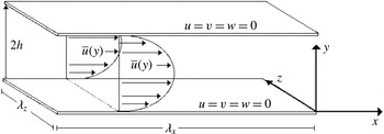
-direction) no-slip and no-penetration conditions were imposed. The flow geometry is presented in figure 1. There are no explicit boundary conditions for vorticity at the wall. This has to be calculated ensuring consistency with the velocity boundary conditions and conservation of mass. This formulation has been successfully applied in several investigations on spatial instability in boundary layers and plane Poiseuille flows. More in depth discussion of the current formulation as compared with that of primitive variables can be found in Meitz & Fazel (Reference Meitz and Fazel2000).
Schematic of flow geometry.

For temporal instability, where a periodic boundary condition is used in the streamwise direction, a Fourier decomposition can be used for the
 $x$
and
 $z$
directions. Each Fourier mode was calculated independently, considering a pseudo-spectral approach to the nonlinear terms (Rist & Fasel Reference Rist and Fasel1995). Because of the streamwise periodicity, an iterative procedure had to be employed to apply the vorticity boundary condition at the wall. The procedure was inspired by Marxen (Reference Marxen1998), but was slightly modified so that only the (0,0) Fourier component required iteration.
For the
 $y$
direction, a high-order compact finite difference scheme was used. Points in the interior of the domain were discretized by centred compact finite differences of sixth-order accuracy. Points at the walls and next to the wall were discretized, respectively, by asymmetric schemes of fifth- and sixth-order accuracy, except for the wall vorticity calculation, which used an asymmetric scheme of sixth-order accuracy. Full details of the finite difference method used can be found in Souza, Mendonça & Medeiros (Reference Souza, Mendonça and Medeiros2005). For all Fourier modes, except for the zeroth mode
 $(0,0)$
, the temporal integration was carried out with an explicit fourth-order Runge–Kutta method of four stages (Ferziger & Peric Reference Ferziger and Peric1997).
2.2 Code testing
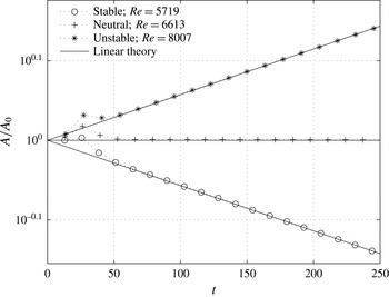
Prior to the study of the nonlinear modulated waves the code was tested by comparison with linear stability theory as well as with the classical nonlinear regimes of TS waves. Figure 2 presents a comparison of the amplitude evolution of the waves as computed by the code with the predictions from the theory. Three test cases using streamwise wavenumber
 $\unicode[STIX]{x1D6FC}=1$
are presented, namely, an unstable, a neutral and a stable wave. After a short initial transient, the wave amplitude evolves as a perfect straight line in the logarithmic plot, the slopes of the lines agreeing remarkably well with theory for all three cases. The initial transient is related to the excitation procedure which used suction and blowing at the wall. It is recognized that it takes some time for the TS wave to form.
Comparison of DNS results (symbols) and theory (line) for three different wave amplitude evolutions.

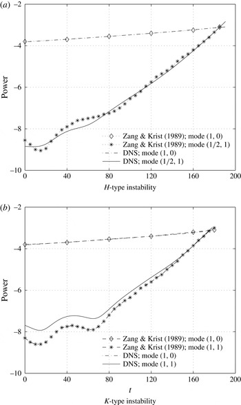
Comparison between DNS results (line) and results from Zang & Krist (Reference Zang and Krist1989) (symbols) for secondary instability.

Tests in the nonlinear regime were done by comparison with direct numerical simulation (DNS) computations reported by Zang & Krist (Reference Zang and Krist1989). Results for the
 $H$
-type instability are given in figure 3(a) while
 $K$
-type instability is shown in figure 3(b). In each picture, only the two-dimensional driving mode and a three-dimensional unstable mode are displayed. The results agree very well. These tests, in combination with tests reported in Silva et al. (Reference Silva, Souza and Medeiros2010), indicated that the code was sufficiently accurate for the studies that followed.
3 The fundamental instability regime
3.1 Evolution of the wave system
As stated previously, the current investigation considers temporal instability. The harmonic point source in a spatial problem (Mack Reference Mack and Kozlov1985) is represented, in the corresponding temporal problem, by a streamwise periodic line source that is excited at time
 $t_{0}$
only. The problem is then specified by a Reynolds number and a streamwise wavenumber
 $\unicode[STIX]{x1D6FC}$
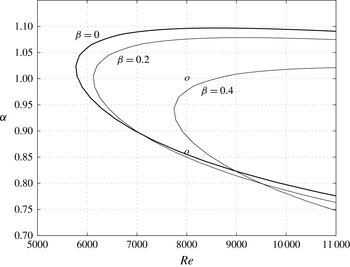
and it is represented by a point in a temporal stability diagram of the flow, figure 4.
Linear stability diagram. The circle at
 $\unicode[STIX]{x1D6FC}=1.0$
indicates the case discussed in this section, the other circle corresponds to the case of § 4.

In the current investigation, a large range of parameters was studied, but, except for the region close to the first branch, the general behaviour was similar (Silva Reference Silva2008). This section deals with the regime observed far from the first branch. In this region the wavetrain is dominated by two-dimensional waves. The results for Reynolds number 8000 and streamwise wavenumber
 $\unicode[STIX]{x1D6FC}=1$
were chosen for discussion as this parameter set was also the object of several investigations of unmodulated waves, such as Zang & Krist (Reference Zang and Krist1989). Figure 4 indicates that this point is well within the unstable region, close to maximum amplification rate for the chosen Reynolds number.
The idea was to study an isolated wave system and, on account of the periodic boundary conditions in the spanwise direction, a study was required. It was found that a spanwise domain of approximately
 $[-100,100]$
non-dimensional units was needed to prevent interaction of the wavepacket with its neighbours, which led to a lowest spanwise wavenumber of
 $\unicode[STIX]{x1D6FD}=0.03$
. Tests were then also performed to verify the number of spanwise modes that would be required to capture the linear and weakly nonlinear activity of the wave system. For code efficiency the number of modes considered were powers of 2. The tests led to 256 modes, which, after using the 2/3 rule to avoid aliasing, provided resolution up to
 $\unicode[STIX]{x1D6FD}=2.55$
. This was enough to capture, besides the linear spectral band, the first and second most important distinct nonlinear bands in the spanwise spectral domain.
All the modes excited had the same streamwise wavenumber, and in the linear and nonlinear regimes the whole signal was contained in that wavenumber, its harmonics and in streamwise independent modes. In view of that, the spectral discretization in the streamwise direction could correspond to
 $\unicode[STIX]{x1D6FC}=1$
and it was found that 16 Fourier modes were sufficient to represent the main features of the flow. In the wall-normal direction a total of 201 points was needed to ensure grid independent results, no grid stretching being employed.
In Fourier space, the line source is represented by a large number of Fourier modes in the spanwise direction, which is what renders the disturbance modulated. For the initial tests a suction and blowing initial condition was constructed from a combination of all resolved spanwise wavenumbers with identical amplitudes. However, in view of the large number of modes, this excitation was too large in physical space and the disturbance became exceedingly nonlinear right at the source. Since high spanwise wavenumber modes are severely linearly damped, it was considered that the excitation could be limited to a band of spanwise modes. The band chosen was
 $[-0.66,0.66]$
which covers modes well beyond the linearly unstable band, the modes being excited at a magnitude of approximately
 $10^{-5}$
. Owing to the nonlinearity of the Navier–Stokes equation, modes in the range
 $\pm [0.7,1.4]$
were excited right at the beginning at the level
 $10^{-10}$
and yet higher spanwise wavenumber modes at the level
 $10^{-15}$
. Despite the very low amplitudes, under some circumstances these jumps in excitation level appeared to have an impact on the nonlinear regime of the disturbances. It was then decided to excite these modes also at a low excitation level, here we used
 $10^{-8}$
, to overcome this nonlinear contribution at the source. This was meant to represent, in some way, a background noise level that is always present in an experiment. However, it was neither uncorrelated nor continuously fed as in a physical experiment, but was actually phase synchronized with the main excitation. The influence of these highly oblique modes is addressed in § 3.2.
The idea was to produce an excitation spectrum as flat as possible and hence prevent any bias towards a particular part of the resolved spectrum. Nevertheless, the blowing and suction excitation favoured the lower spanwise wavenumbers. It was then decided to use the actual TS eigenfunctions to excite the flow as an initial condition applied throughout the computational domain. This worked very well and brought the extra advantage of preventing any initial transient that would have appeared if the excitation had a generic shape in the
 $y$
direction.
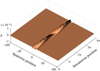
Figure 5 displays the initial condition for the disturbance velocity streamwise component on a plane parallel to the wall at
 $y=0.15h$
, which is close to the maximum amplitude of the eigenfunction of the two-dimensional wave composing the system. The maximum amplitude in physical space is below
 $10^{-3}$
. Modulated waves in boundary layers can become nonlinear at amplitudes
 $0.2\times 10^{-2}$
(Medeiros & Gaster Reference Medeiros and Gaster1999a
; Medeiros Reference Medeiros2004b
), hence, in the current study, it was considered important to work with wave amplitudes that started below that level.
Initial condition for disturbance velocity streamwise component along spatial coordinates
 $x$
and
 $z$
at
 $y=0.15h$
.
 $A$
indicates amplitude.

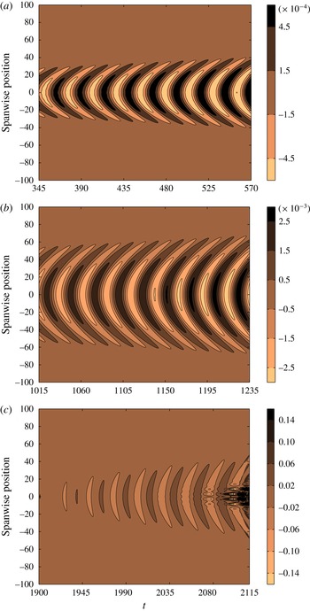
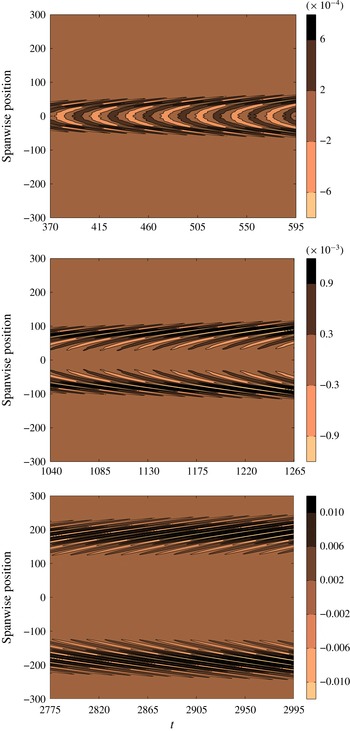
Figure 6 displays the time evolution of the wave system at a fixed
 $x$
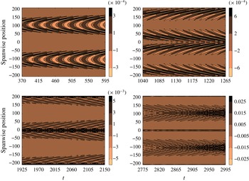
station. The top and middle frames display essentially a linear behaviour. The waves exhibit the characteristic crescent shape, continuously growing in time and progressively spreading over a wider portion of the spanwise domain. In the bottom frame, some nonlinear activity is already present at time
 $t=1950$
. It is characterized by an offset in the plot, that is, a distortion in the base flow, and as a consequence, the positive and negative contour levels become asymmetric. This nonlinearity is however very mild. At approximately
 $t=2035$
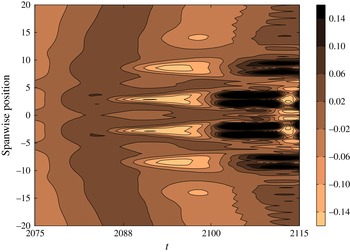
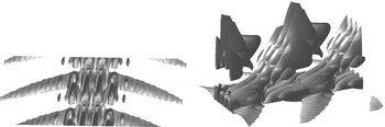
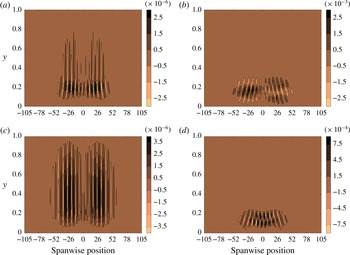
, it is possible to identify another nonlinear activity around the centreline. This was very localized in space and explosive in time. It is characterized by the formation of aligned regions of large and small amplitude across the span and progressively spreads in this direction. Figure 7 displays a close-up view of this nonlinear activity. Figure 8 shows iso-surface plots of the spanwise vorticity of the same structure. These plots show that the structure resembles the
 $\unicode[STIX]{x1D6EC}$
-structures that characterize nonlinear stages of transition of unmodulated waves, but here they are very localized in span.
Temporal evolution of streamwise velocity component of the wave system at an arbitrary streamwise position, at
 $y=0.15h$
and across the span. Each frame covers a selected range of non-dimensional time.

Close-up view of late nonlinear stages of figure 6.

Surface plots of spanwise vorticity at later stages of nonlinear regime.

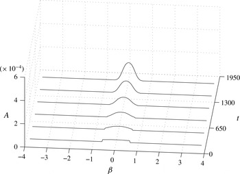
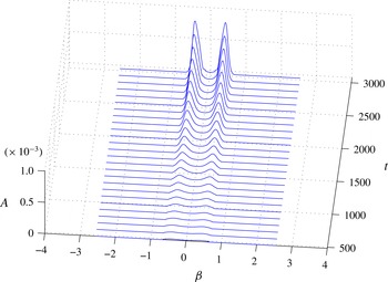
Figure 9 displays the wave system linear evolution in spanwise wavenumber space for the fundamental modes, that is, modes of the fundamental streamwise wavenumber, namely,
 $\unicode[STIX]{x1D6FC}=1$
. The first time station shows that a portion of the spectrum was excited at a higher constant amplitude. It is important to note that, at the end of the linear regime, all modes that significantly contribute to the spectra were excited at the same level at the origin. The evolution reduces the spectral width of the band and favours the low spanwise wavenumbers.
Spanwise spectral evolution of fundamental modes for streamwise disturbance velocity in the linear regime.

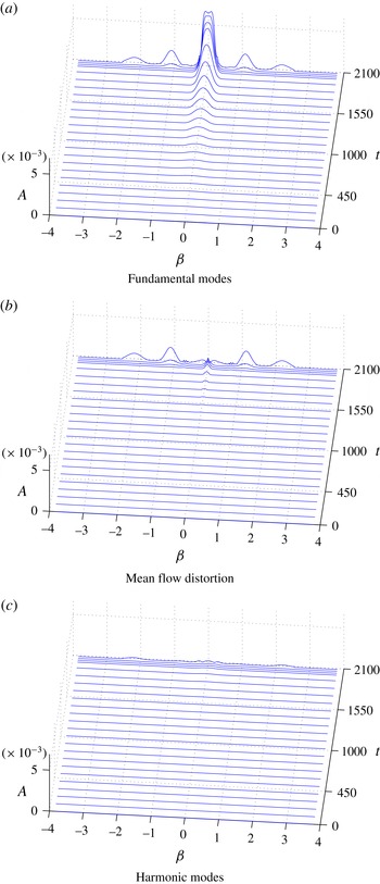
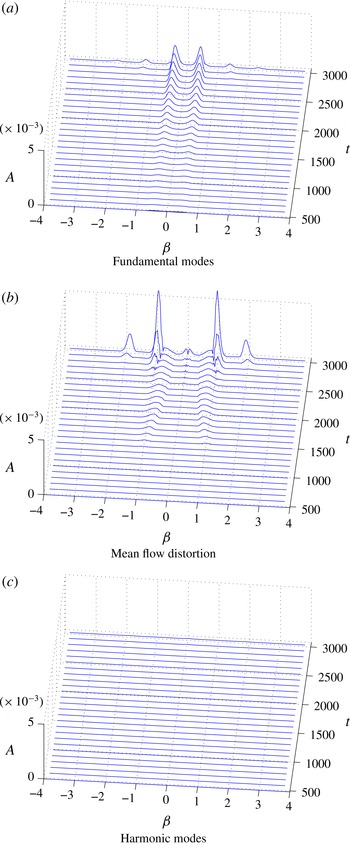
Figure 10 shows the temporal evolution in spectral domain beyond the linear regime. Figure 10(a) is for the fundamental modes, namely,
 $(\unicode[STIX]{x1D6FC}_{0},\unicode[STIX]{x1D6FD})$
, figure 10(b) for the
 $(0,\unicode[STIX]{x1D6FD})$
modes and figure 10(c) for the
 $(2\unicode[STIX]{x1D6FC}_{0},\unicode[STIX]{x1D6FD})$
modes. Figure 10(b,c) is associated exclusively with nonlinear interactions in the process. The earliest nonlinear activity observable in the plot was for modes
 $(0,\unicode[STIX]{x1D6FD})$
around time
 $=$
1600, figure 10(b). This is characterized by a small band around
 $\unicode[STIX]{x1D6FD}=0$
and is the Fourier space manifestation of the mean flow distortion observed in figure 6. The
 $(0,\unicode[STIX]{x1D6FD})$
mode nonlinear activity was relatively weak and no significant effect was yet observed in the fundamental band
 $(\unicode[STIX]{x1D6FC}_{0},\unicode[STIX]{x1D6FD})$
which essentially maintained a linear behaviour up to time
 $=$
2000. After that, the
 $(\unicode[STIX]{x1D6FC}_{0},\unicode[STIX]{x1D6FD})$
modes show spectral bands different from the linear one. Initially these spectral bands were centred approximately around
 $\unicode[STIX]{x1D6FD}=\pm 1.1$
and, soon after, another band appeared at approximately
 $\unicode[STIX]{x1D6FD}=\pm 2.2$
. The growth of these modes was explosive, much larger than that of the linear regime. Both spanwise spectral bands are present for the
 $(0,\unicode[STIX]{x1D6FD})$
modes and, albeit small, the band around
 $\unicode[STIX]{x1D6FD}=2.2$
is also observed for modes
 $(2\unicode[STIX]{x1D6FC}_{0},\unicode[STIX]{x1D6FD})$
. In the study, spanwise grid independence tests were carried out by comparing these results with those from a less refined simulation with twice the grid spacing in the
 $z$
direction. All results were virtually independent of the grid for the entire spanwise spectral domain of the less refined case, in particular for the later nonlinear stages. The less refined simulation domains falls within
 $\unicode[STIX]{x1D6FD}=\pm 2.55$
, and the following analysis will be restricted to this spectral domain. We, nevertheless decided to use the most refined results in figures 10 and 11 because we expect them to be more complete, but studies in § 3.2 used the less refined grid.
Spanwise spectral evolution for streamwise disturbance velocity.

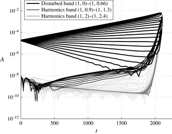
Evolution of fundamental modes for different bands of spanwise wavenumber.

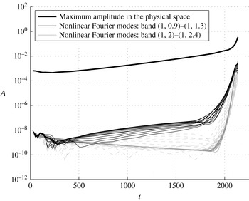
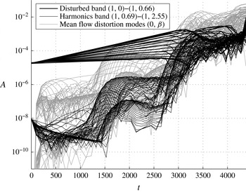
Figure 11 shows the evolution of the fundamental modes grouped in selected bands. The thick black line indicates modes that where excited at the level
 $2\times 10^{-5}$
,
 $\unicode[STIX]{x1D6FD}=[0,0.66]$
. Clearly the modes covered the linearly unstable modes as well as modes that were highly damped. The unstable and least stable modes exhibit exponential growth or decay practically over the entire simulated time period. The range
 $\unicode[STIX]{x1D6FD}=[0.9,1.3]$
is indicated by the thin black line. This modes compose the first nonlinear band observed in the spanwise spectra of the fundamental modes. The second nonlinear band is composed of the modes
 $\unicode[STIX]{x1D6FD}=[2.0,2.4]$
and it is represented by grey lines. Other fundamental modes not shown do not belong in the linear and nonlinear dominant bands. The highly oblique modes were excited at
 $10^{-8}$
. From the beginning they display very mild growth or decay, but at time approximately 1700 a strong growth is observed for the two selected bands. It is interesting to note that, by time 1700, the most oblique waves excited at the higher level reached amplitudes similar to those of waves that were not initially excited at the highest level. This was considered an indication that exciting a wider spanwise wavenumber range at the highest level would not significantly affect the results.
The large growth rates, the association between nonlinear fundamental and streak modes and the
 $\unicode[STIX]{x1D6EC}$
-vortex structures suggested that the observed nonlinear behaviour was governed by secondary instability of the fundamental type, also called the
 $K$
-type instability. This hypothesis was then further investigated. In order to verify the existence of secondary instability, the nonlinear modulated wavetrain was compared with the fundamental secondary instability of the dominant two-dimensional wave composing the spanwise modulated wave system. There are various ways of producing secondary instability results. Nowadays, simulations of this type are relatively fast and DNS can be used efficiently to produce them. Accordingly, several simulations were carried out for
 $Re=8000$
. For each simulation, a two-dimensional wave with
 $\unicode[STIX]{x1D6FC}=1$
and initial amplitude
 $10^{-4}$
and a pair of oblique symmetrical waves with initial amplitude
 $1\times 10^{-5}$
were excited. For each simulation a different spanwise wavenumber of the oblique mode was used, changing at
 $\unicode[STIX]{x1D6FD}$
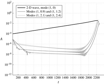
-intervals of 0.3. The set of simulations covered the spectral bands displayed in figure 10. The results of some of these simulations are collected together in figure 12. Initially the oblique waves experience a strong decay and by the time the secondary instability sets in their amplitudes are approximately
 $10^{-8}$
which is similar to that of the modulated wave case studied, figure 11. A qualitative comparison of growth rates in figures 11 and 12 suggests similar growth rates. Nevertheless figure 12 shows that the instability is triggered when the two-dimensional wave reaches an amplitude of approximately
 $10^{-2}$
, while for the modulated wave system the strong nonlinear behaviour starts when the dominant, two-dimensional wave is at an amplitude of approximately
 $10^{-3}$
.
Evolution of
 $K$
-type secondary instability modes driven by a two-dimensional wave at larger amplitude for
 $\unicode[STIX]{x1D6FC}=1$
. Each simulation involved only the two-dimensional wave and a pair of oblique waves. The results of simulations for the different spanwise wavenumbers were combined in a single figure. The two-dimensional wave is indicated by the thick black line and oblique modes by the thin lines.

Evolution of modes
 $0.9\leqslant \unicode[STIX]{x1D6FD}\leqslant 2.4$
composing the modulated wave system and of wave amplitude along the centreline of the wave system.

An important feature observed in figure 6 is that the nonlinear activity associated with these oblique modes was very localized around the wave system centreline. It is possible that the highly oblique waves with large spanwise wavenumbers interact with the wave system as if the latter were an effectively two-dimensional wave. Around the centreline, the modulated wave system reaches a shallow amplitude maximum and this amplitude may provide an estimate of the amplitude of an effective two-dimensional wave driving the system. Figure 13 presents the evolution of the discussed nonlinear modes as well as the centreline amplitude evolution. The growth rate of the maximum amplitude of the wave system (which in this parameter set is at the centreline) is substantially lower than that of the two-dimensional wave in the wave system, compare figures 12 and 13. This is associated with the fact that the two-dimensional wave has the maximum growth rate of all waves composing the system. The wave system growth rate comes from a composition of the growth rates of all waves in the system, and it is lower than the maximum. It is remarkable that the beginning of the strong oblique wave amplification corresponds to a centreline amplitude of
 $10^{-2}$
, in agreement with
 $K$
-type instability of unmodulated waves, figure 12. The result lends very strong support to the notion of an effective wave amplitude. This concept has already been proposed by de Paula et al. (Reference de Paula, Würz, Krämer, Borodulin and Kachanov2013) in the context of streamwise modulation, where the effective amplitude was also found to be the maximum.
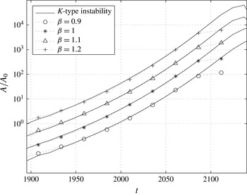
Yet a more conclusive demonstration of existence of secondary instability is the agreement of the growth rates. Figure 14 displays the evolution of oblique modes driven by the
 $K$
-type instability of a two-dimensional wave (from figure 12) and the evolution of the corresponding oblique modes in the spanwise modulated wave. Secondary instability cannot establish the initial amplitude of the unstable wave, but only the growth rate. In order to facilitate comparison, the curves were arbitrarily shifted in the vertical direction.
The agreement is remarkable for all modes and up to very late stages of the simulation. It is important to note, in passing, that the growth rate of the centreline amplitude is different from that of a corresponding two-dimensional wave (compare figures 12 and 13). Therefore, the driving wave of each of the two systems would not display identical amplitude levels throughout the secondary instability regime. Since the secondary instability growth rates are dependent on the driving wave amplitude, it may sound surprising that the agreement is so good. This might, however, be associated with the fact that the phenomenon is so fast that such differences become irrelevant.
Comparison of evolution of modes subject to classical
 $K$
-type secondary instability (lines) with corresponding modes in the modulated wave system (symbols), for spanwise wavenumbers in the first (lower spanwise wavenumber) nonlinear fundamental spectral band.

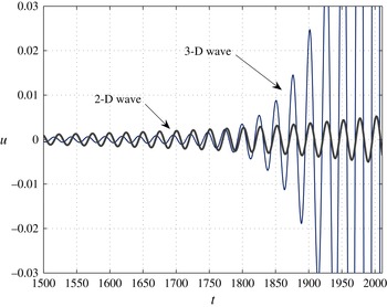
Time evolution, at position
 $z=2$
, of a two- and a three-dimensional wave in the modulated wavetrain. For clarity, the three-dimensional wave amplitude is multiplied by
 $2.5\times 10^{4}$
.

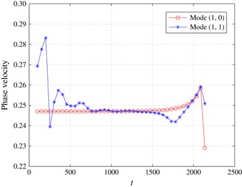
Time evolution of the phase speed of a two- and a three-dimensional wave with
 $\unicode[STIX]{x1D6FD}=1$
in the modulated wavetrain.

The secondary instability is associated with a phase synchronization of resonant waves. Figure 15 displays, at position
 $z=2$
which corresponds to the centre of a
 $\unicode[STIX]{x1D6EC}$
-structure in figure 7, the evolution of the streamwise velocity components of the two-dimensional wave in the wave system as well as that of an oblique wave. The oblique wave chosen had
 $\unicode[STIX]{x1D6FD}=1$
, which is among the most growing nonlinear modes. For clarity, the amplitude of the oblique wave is multiplied by
 $2.5\times 10^{4}$
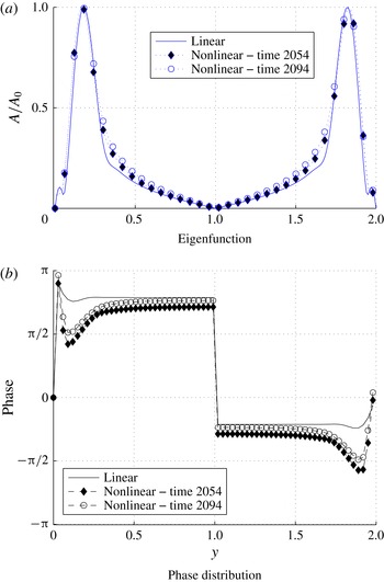
. Clearly a phase synchronization starts to take place at approximately time 1700, whereas perfect synchronization occurs shortly after time 1900. Over this period the oblique wave experiences a substantial increase in growth rate. Phase synchronization can also be assessed by the phase speed, figure 16. Already at time 700 the phase speeds of the waves are very similar. At approximately time 1500, the phase speed of the three-dimensional mode changes substantially, but eventually it adjusts back to the two-dimensional wave speed. The phase speed variation corresponds to the period in which phase synchronization in observed in figure 15. The speed modification is that required for the phase of the three-dimensional wave to adjust to that required by the instability. Prior to the phase synchronization, the waves already have similar speeds. This is inconsistent with a linear behaviour for the three-dimensional wave and will be addressed later in the paper. Theory predicts that the shape of the secondary instability modes resemble very closely the corresponding eigenfunction of the linear instability regime (Herbert Reference Herbert1988). Comparisons of such mode shapes and phase distribution are displayed in figure 17. The agreement is very good, even at very late stages of the simulation.
Comparison of amplitude and phase distribution of a linear instability eigenfunction (solid line) with that of a nonlinear mode in
 $K$
-type regime in the modulated wave system. Comparison is made for streamwise velocity components with
 $\unicode[STIX]{x1D6FD}=1$
, and the nonlinear wave is captured at times 2054 (diamonds) and 2094 (circles).

There remains to be investigated the second nonlinear fundamental band, that around
 $\unicode[STIX]{x1D6FD}=2.2$
in figure 10. Figure 18 displays the evolution of oblique modes driven by the
 $K$
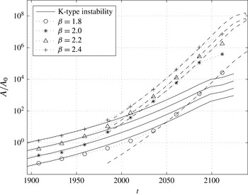
-type instability of a two-dimensional wave (from figure 12) and the evolution of corresponding oblique modes composing the second nonlinear fundamental band in figure 10. As in figure 14, the curves are shifted arbitrarily in the vertical direction. Initially the wave evolution conforms very well with the
 $K$
-type instability. At a later stage the growth rates become much larger. At this stage however, the wave growth rates agree very well with twice the growth rates of
 $K$
-type instability waves with half their spanwise wavenumber. In view of the fact that the growth at this stage is substantially larger than the previous one, the result provides a strong evidence that these waves are driven directly by nonlinear interaction between the waves of the first nonlinear fundamental band.
 $K$
-type instability modes are composed of fundamental oblique modes and streak modes of the same spanwise wavenumbers. The fundamental modes of this second nonlinear band could result from a nonlinear interaction between the fundamental and the streak modes of the
 $K$
-type instability.
Comparison of evolution of modes subject to classical
 $K$
-type secondary instability (solid lines) and of corresponding modes in the modulated wave system (symbols), for spanwise wavenumbers in the second (higher spanwise wavenumber) nonlinear fundamental spectral band. Dashed lines represent evolution at twice the growth rate of modes with half the spanwise wavenumber.

3.2 Origin of secondary instability modes
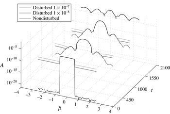
Secondary instability can enhance the growth of modes already existing in the flow, but it cannot produce them. In the current study the wavenumbers that eventually took part in the secondary instability regime were excited at the origin at a lower level. This excitation was meant to represent, in a restricted way, a noise floor. In view of this limitation, this issue was further addressed. Figure 19 presents the spectral evolution of the fundamental modes in the wave system subject to three different excitation cases. The low spanwise wavenumber modes were excited at
 $10^{-5}$
for all cases. For one simulation, the more oblique modes were excited at
 $10^{-7}$
, for another,
 $10^{-8}$
and in a third simulation these were not excited other than by the discretization error. The figure shows that, progressively, all three cases lead to identical spectra. Clearly, the seeds for the secondary instability were not the disturbances excited at the source, but were produced nonlinearly prior to the secondary instability. The fact that the resonant three-dimensional waves are already nonlinear prior to the secondary instability is consistent with figure 16 of the previous section, where even at early stages the three-dimensional waves do not display the phase speed predicted by the linear theory. Production of modes in modulated wave systems has been reported for subharmonic waves (Medeiros & Gaster Reference Medeiros and Gaster1999b
; Craik Reference Craik2001; de Paula et al.
Reference de Paula, Würz, Krämer, Borodulin and Kachanov2013) in the context of modulated waves.
Spectral evolution of the modulated wave system subjected to the different excitation levels for the very oblique fundamental modes.

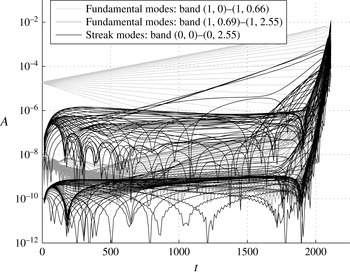
Quadratic nonlinear interaction of fundamental modes cannot produce waves of the fundamental streamwise wavenumber. They can, however, produce streak modes, which would have a projection on the
 $K$
-type instability modes (note that
 $K$
-type modes contain a streak mode component). Figure 20 shows that indeed nonlinear streak modes are much larger than nonlinear fundamental modes throughout the evolution. These streak modes are produced from the interaction of fundamental modes in the modulated wave system. These modes do not have identical phase speeds, which leads to the observed mode beating, in particular for the more oblique modes that are produced from the interaction of more spectrally distant linear modes. The figure also shows three streak modes with substantially larger growth rates. These are the lowest wavenumber modes, including the
 $(0,0)$
mode, and will be addressed later in the paper.
Evolution of the modulated wave system. Fundamental modes
 $0\leqslant \unicode[STIX]{x1D6FD}\leqslant 0.66$
, light grey lines; fundamental modes
 $0.69\leqslant \unicode[STIX]{x1D6FD}\leqslant 2.55$
, dark grey lines; streak modes
 $0\leqslant \unicode[STIX]{x1D6FD}\leqslant 2.55$
, black lines.

Medeiros (Reference Medeiros2004b
) indicates the existence of
 $K$
-type instability in the nonlinear evolution of a spanwise modulated wavetrain in a flat plate boundary layer. Indirect evidence suggested that the seeds for the
 $K$
-type instability arise from previous nonlinear interaction producing streak modes. As explained by Schmid & Henningson (Reference Schmid and Henningson1992), streaks are often associated with streamwise vorticity. Medeiros (Reference Medeiros2004b
) recasts an equation proposed by Elofsson & Alfredsson (Reference Elofsson and Alfredsson1998) in a restricted version applied to the spanwise modulated wavetrain in the flat plate boundary layer, for the streamwise vorticity produced by the nonlinear interaction of the linear modes in the wave system. Adapting to the current parallel flow and under temporal evolution, that equation becomes
 $$\begin{eqnarray}\displaystyle \frac{\unicode[STIX]{x2202}\unicode[STIX]{x1D709}_{2}}{\unicode[STIX]{x2202}t}-\frac{1}{Re}\unicode[STIX]{x1D6FB}^{2}\unicode[STIX]{x1D709}_{2} & = & \displaystyle \frac{\unicode[STIX]{x2202}^{2}}{\unicode[STIX]{x2202}z^{2}}\left(v^{\prime }w^{^{\prime }\ast }+v^{^{\prime }\ast }w^{\prime }\right)-\frac{\unicode[STIX]{x2202}^{2}}{\unicode[STIX]{x2202}y^{2}}(v^{\prime }w^{^{\prime }\ast }+v^{^{\prime }\ast }w^{\prime })\nonumber\\ \displaystyle & & \displaystyle +\,2\frac{\unicode[STIX]{x2202}^{2}}{\unicode[STIX]{x2202}z\unicode[STIX]{x2202}y}(v^{\prime }v^{^{\prime }\ast })-2\frac{\unicode[STIX]{x2202}^{2}}{\unicode[STIX]{x2202}z\unicode[STIX]{x2202}y}(w^{\prime }w^{^{\prime }\ast }),\end{eqnarray}$$
where
 $\unicode[STIX]{x1D709}_{2}$
is the streamwise vorticity first nonlinear correction.
 $v^{\prime }$
and
 $w^{\prime }$
are, respectively, the wall-normal and spanwise velocity components of the linear TS wave,
 $Re$
is the Reynolds number and
 $^{\ast }$
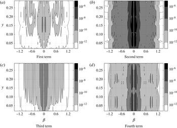
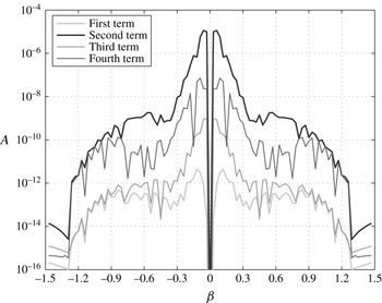
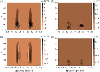
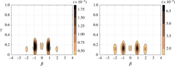
denotes complex conjugate. The equation shows that the spanwise wavenumber of the streamwise vorticity, and hence of the streaks, should be given by the forcing terms. Figure 21 shows the four nonlinear forcing terms for the spanwise modulated wave in plane Poiseuille flow at time
 $t=1000$
. Figure 22 shows a cut of the frames of figure 21 at
 $y=0.07h$
. As in the boundary layer case (Medeiros Reference Medeiros2004b
), for the plane Poiseuille flow the second term is dominant.
Nonlinear forcing terms of (3.1), in spanwise wavenumber
 $\times$
wall-normal direction planes, at time 1000.

Nonlinear forcing terms of (3.1), in spanwise wavenumber
 $\times$
wall-normal direction planes, at time 1000 and
 $y=0.07h$
.

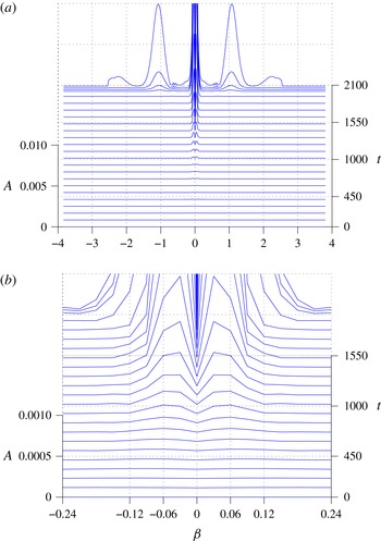
Figure 23 shows the spectral evolution of the
 $\unicode[STIX]{x1D6FC}=0$
modes composing the streamwise vorticity in the modulated wave. Any content in these modes is the outcome of some nonlinear action. Already at time 1000 there are distinct spectral bands. The zoomed view indicates their dominant spanwise wavenumber. They correspond to the steak modes that, in addition to mode
 $(0,0)$
, present the higher growth rates in figure 20. They closely match the spanwise wavenumbers of the second forcing term in (3.1). Clearly, this direct forcing is the governing nonlinear activity prior to the secondary instability. It is apparent that these wavenumbers are quite different from those that can resonate in the secondary instability regime. Nevertheless, the signal is modulated and, as shown in figure 22, spreads over a wide portion of the spanwise wavenumber domain. At
 $\unicode[STIX]{x1D6FD}$
around 1.0, the first nonlinear band, both the second and the third term contribute significantly.
Spectral evolution of the
 $\unicode[STIX]{x1D6FC}=0$
modes composing streamwise vorticity in the modulated wave. Bottom panel is a zoomed version.

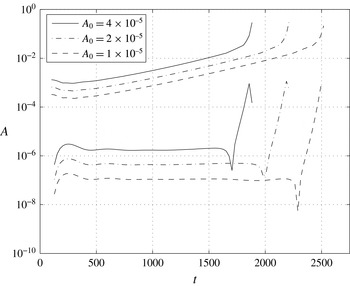
Tests were also carried out for three different excitation levels (
 $1\times 10^{-5}$
,
 $2\times 10^{-5}$
and
 $4\times 10^{-5}$
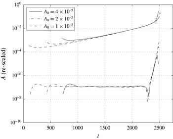
) of the modes composing the fundamental wave system. Figure 24 shows the amplitude evolution along the centreline and the amplitude of the dominant nonlinear oblique mode (1, 1.02) for the three cases in the same plot. As the amplitude increases the secondary instability starts earlier. Figure 25 shows the same data, but with the evolution for each amplitude shifted in time to display a collapse. The evolution of the oblique modes were rescaled based on the square of the initial amplitude. In other words, the curve for amplitude
 $2\times 10^{-5}$
was divided by 4 and that for amplitude
 $4\times 10^{-5}$
, divided by 16. The results show a remarkably good collapse for all curves. They demonstrate that the oblique seeds scaled with the square of the amplitude of excitation, consistent with the arguments raised above. The collapse also shows that the threshold for strong growth is the same for all cases and so is the growth rate, also consistent with the
 $K$
-type instability. It is interesting that for the boundary layer the amplitude of the
 $K$
-type modes scaled with the cubic power of the excitation amplitude (Medeiros Reference Medeiros2004b
). This is different from the current result but it is not known a priori what could be the reason for this.
Evolution of amplitude along the centreline and amplitude of mode (1, 1.02) at different excitation levels.

As in figure 24, but time shifted and amplitude rescaled to show collapse.

4 The oblique transition regime
As anticipated, for a spanwise modulated wavetrain in plane Poiseuille flow, the nonlinear evolution in general can be assigned to the secondary instability of the fundamental type, except close to the first branch of the instability loop. This section investigates this region of the parameter space. The same Reynolds number (based on the maximum speed in the channel and half the channel height) was used, namely,
 $Re=8000$
. The initial amplitudes used and the range of spanwise wavenumbers excited were also identical to those of the previous study. The only parameter changed was the streamwise wavenumber, which here was 0.86, bringing the test case close to the first branch of the instability loop (see figure 4). In that region, for a given streamwise wavenumber, the three-dimensional waves are more unstable than the two-dimensional one. This is a direct consequence of Squire’s theorem (Squire Reference Squire1933). In fact, in the current test case, the two-dimensional wave was essentially neutral, but the general conclusion held as long as the three-dimensional wave was sufficiently dominant.
The resolution used was also in general identical to that of the previous study, namely, 201 points in the wall-normal direction, 16 modes in the streamwise wavenumber dimension. Once more tests indicated that no subharmonics were active in the process, therefore the lowest non-zero streamwise wavenumber simulated was that excited. Owing to the spanwise periodic boundary condition, the spectral resolution requirements in that direction were related to the spanwise separation between wavetrains. The number of modes was chosen to capture all the relevant flow features. This spanwise spectral resolution is further discussed below.
The excitation procedure was again identical to that shown by figure 5, namely, a patch of TS waves were placed in the flow at some initial time. The unstable and least stable modes were excited at a higher amplitude,
 $2\times 10^{-5}$
while the other modes had an amplitude of
 $1\times 10^{-8}$
.
Figure 26 displays the evolution of the streamwise velocity of the wave system in Fourier space at
 $y=0.15h$
. The results confirm the expectation that, in the linear regime, at say time equals 1500, indeed a three-dimensional wave was the most unstable mode in the case
 $\unicode[STIX]{x1D6FD}=0.48$
.
Time evolution of fundamental Fourier modes for
 $u$
-velocity.

Time evolution of the
 $u$
-perturbation velocity of a spanwise modulated wavetrain in the plane Poiseuille flow at
 $y=0.15h$
and arbitrary
 $x$
.

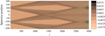
Figure 27 exhibits the evolution in physical space. The figure shows the streamwise perturbation velocity at
 $y=0.15h$
in a spanwise
 $\times$
time plane for a given streamwise position. Since the signal is periodic in the
 $x$
direction, the figure provides enough information about the evolution of the wave system. The disturbance splits into two patches that propagate in opposite oblique directions. The dominant mode in the packet is the most unstable mode and gives the dominant vector phase velocity, which is related to the wave crests. The propagation of the centre of the packet, its maximum amplitude, is related to the vector group velocity of the dominant mode. These velocity vectors in general are not parallel to each other. Since the picture is a time
 $\times$
span plane, the direction of the wave crests relative to these velocity vectors are not directly seen in the picture as they would in a streamwise
 $\times$
span plane. However, because the dominant wave is oblique, the wave patches also travel obliquely.
Figure 27 indicates also that the signal is consistent with linear theory up to relatively high amplitudes. In this context, nonlinear activity could also be related to mean flow distortion or harmonics. However, the spectral evolution of these modes (not shown) revealed very little activity. Since the amplitude was well above 1 %, it was concluded that the nonlinear activity of this type of wave system was very weak or restricted to very large wave amplitude.
In view of the fact that the isolated patches did not display relevant nonlinear behaviour and that, in a practical situation, the oblique propagation could facilitate spanwise interaction, it was considered that, under these circumstances, the interaction of spanwise modulated wavetrains could be a possible scenario leading to transition.
Figure 28 displays the time evolution of interacting wavetrains in a time
 $\times$
span plane for
 $y=0.15h$
and an arbitrary
 $x$
. Selected periods of the evolution are shown in more detail in figure 29, with contour levels chosen to show the more relevant features of the different stages of the evolution. If the patches merge an interaction can take place. If the amplitudes of the patches are too small, (say, at time equals 2000) they do not seem to interact nonlinearly. The resulting pattern is essentially given by the sum of the waves which return to isolated patch pattern once they separate. If, on the other hand, the wave amplitude is sufficiently large, a nonlinear interaction is observed with the production of longitudinal streaks. It is important to note that this amplitude is yet significantly smaller than that required for the isolated patch to behave nonlinearly.
Time evolution of
 $u$
-perturbation velocity of interacting spanwise modulated wavetrains in plane Poiseuille flow at
 $y=0.15h$
and at a fixed
 $x$
, in physical space. Note that the simulation is periodic in the spanwise direction and two spanwise periods are shown.

Selected periods of the evolution shown in figure 28.

Figure 30 shows the time evolution of the signals in Fourier space. Results are given for the fundamental streamwise wavenumber, the mean flow distortion and its first harmonic. As already mentioned, the subharmonic frequency did not play a role here. Likewise, the higher harmonics were also not relevant. Nonlinear activity was first and mostly observed in the mean flow distortion. For the mean flow distortion, the spanwise wavenumber of the first nonlinear band was approximately twice the dominant spanwise wavenumber of the linear regime and, for the fundamental wavenumber, it was approximately three times. Later, other bands arise in a consistent fashion. The whole picture is very different from that observed in the previous section. The scenario is very characteristic of oblique transition and, together with the pattern in physical space, was considered enough evidence that this was the mechanism driving the nonlinear behaviour.
Time evolution of Fourier modes for
 $u$
-velocity.

Interesting information can also be obtained from the time evolution of the signals in Fourier space, figure 31. The nonlinear activity was characterized by a stepwise increase in amplitude for various modes. Each step corresponds to a period over which the patches merged and interacted. As seen, even for very small amplitude there was an interaction of the same nature as that for larger amplitudes. Nevertheless, for small amplitudes this interaction was not enough to lead to transition or even leave any significant scar in the signal. It was only for large amplitudes that the interaction was important. Oblique transition was not reported to have a threshold amplitude as for secondary instability. Likewise, tests with other amplitudes (not reported here) did not show any threshold too.
Temporal evolution of Fourier modes.

In order to further substantiate the action of the oblique transition in the scenario, some calculations were carried out. Oblique transition is characterized by the forcing of longitudinal vorticity via Reynolds stress interactions and is governed by (3.1). The four non-homogeneous terms are presented in figure 32 for an early time, when the patches are isolated and in figure 33, for time 3000, when they are interacting. The figures show that the dominant terms are the second and fourth ones. There are interesting differences between the terms for the isolated and interacting stage. The terms are inclined differently and the sign is changed.
Magnitude distribution of inhomogeneous (a–d) terms of (3.1) in physical space for an early time.

Magnitude distribution of inhomogeneous (a–d) terms of (3.1) in physical space for a late time.

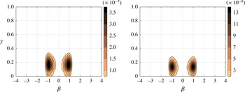
Figures 34 and 35 show the dominant terms in Fourier space. The dominant spanwise wavenumber for both terms at both times is approximately
 $\unicode[STIX]{x1D6FD}=0.9$
, which is twice the dominant spanwise wavenumber in the linear regime. As the spanwise modulation is very weak, the spectral bands are relatively sharp, resembling an unmodulated case.
Magnitude distribution of the dominant non-homogeneous (2 and 4) terms of (3.1) for an early time in Fourier space.

Magnitude distribution of the dominant non-homogeneous (2 and 4) terms of (3.1) for a late time in Fourier space.

5 Final remarks
The paper reports on a numerical investigation of spanwise modulated TS waves. As extensively discussed in the paper, the variation of the local Reynolds number in an evolving wall shear flow causes a gradual variation of the most unstable modes which hinders the interpretation of results of broadband, modulated disturbances. In order to circumvent this difficulty, the constant Reynolds number, plane Poiseuille flow was chosen as the base flow. In doing so, perfect agreement was obtained for the several analyses performed, a feature that would not have been possible if Reynolds number were not constant. Moreover, it was possible to study the phenomenon at fixed points in the linear stability diagram and investigate aspects such as proximity to the first or second branches of the instability loop. Accordingly, two nonlinear regimes were observed. One takes place when the wave system is dominated by a two-dimensional wave, occurring for almost the entire
 $Re\times \unicode[STIX]{x1D6FC}$
parameter space. The other occurs if three-dimensional waves dominate in the packet, which characterize the region close to the first branch of the instability loop, where, in an incompressible framework, three-dimensional waves can be the most unstable ones.
In the first regime, the most salient nonlinear activity is
 $K$
-type instability. In physical space, the phenomenon is very localized at the centre of the wave system. The primary wave driving the instability was not the two-dimensional wave composing the wave system but, rather, an effective two-dimensional wave with an amplitude equal to the maximum amplitude of the wave system. This was demonstrated by perfect agreement between modulated and corresponding unmodulated results for threshold amplitudes and nonlinear growth rates. The seeds for the
 $K$
-type modes originated from previous nonlinear quadratic interaction of the primary modes which produced longitudinal streaks. Results were presented for other excitation amplitudes and showed perfect collapse if scaled appropriately. Almost simultaneously with the fundamental instability, another nonlinear fundamental band arises accompanied by a streak mode band. These are spanwise wavenumber harmonics of the fundamental instability modes. Initially they grow at their fundamental instability growth rates, but later, they consistently exhibit twice the growth rate of their spanwise wavenumber subharmonics. Again, perfect agreement with the predicted growth rates were observed.
In the regime close to the first branch of the instability loop, during the linear stage the wave system splits into two patches that travel obliquely at opposite angles. These patches are very resilient to nonlinear activity if they remain isolated. If there is spanwise interaction of such patches, oblique transition sets in. This was clear from the flow structure observed in physical space, including the formation of longitudinal streaks, and the hierarchy of modes observed in Fourier space. Calculations of the forcing terms driving this nonlinear activity also supported the conclusions and gave further insight into the phenomenon.
The results of the first regime are in qualitative agreement with many features observed in a similar experiment in a boundary layer (Medeiros Reference Medeiros2004b
), except for the amplitude scaling of the
 $K$
-type modes, which for the plane Poiseuille flow was quadratic and for the boundary layer was cubic. It is remarked that Medeiros (Reference Medeiros2004b
) did not compare growth rates and threshold amplitudes. Moreover, since the boundary layer does not have a constant Reynolds number, perfect collapse of rescaled results from excitations of different amplitudes would not be expected. Furthermore, since a typical
 $\unicode[STIX]{x1D6FC}$
in the plane Poiseuille flow is approximately 10 times that of the boundary layer while the corresponding unstable
 $\unicode[STIX]{x1D6FD}$
ranges are similar, the plane Poiseuille flow has a much weaker three-dimensional character. This is reflected in the fact that the fundamental linear and nonlinear bands are very distinct in the plane Poiseuille flow case while for the boundary layer they may overlap (Medeiros Reference Medeiros2004b
). These aspects might have an impact on the packet evolution. Regarding the second regime, it is possible for the boundary layer to produce wave systems dominated by three-dimensional waves, in particular for compressible flows, but packet splitting has not been reported in such flows. Nevertheless, spanwise interaction of packets has been considered relevant in boundary layers close to transonic speeds (Martinez, Gennaro & Medeiros Reference Martinez, Gennaro and Medeiros2015).
Wave modulation is an unavoidable ingredient of natural conditions. Overall, the results indicated that the nonlinear regime of these modulated waves are, essentially, governed by the same nonlinear regimes observed for unmodulated waves. This is interesting because modern transition prediction tools rely on established unmodulated wave nonlinear regimes. Moreover, the results point to directions in which such tools may be further improved. One aspect is that the seeds for secondary instabilities in the modulated case arise from the quadratic interaction of the primary modes composing the packet. This behaviour differs from the unmodulated scenario where the secondary instability seeds either are artificially excited or arise from the background noise. In other words, the evolution of the modulated wave system depends only on the initial content in and around the linearly unstable band, which in turn produces the nonlinear bands. Also, the threshold for secondary instability of modulated waves agrees with that of unmodulated ones. Nevertheless, the important amplitude is not that of an isolated two-dimensional mode, but that observed along the wavepacket centreline. Owing to the dispersive effects, the growth of the centreline amplitude of the wave system is much lower than that of a corresponding two-dimensional wave. Another interesting aspect is that, in both regimes, the nonlinear activity was very localized in the spanwise direction and explosive in time, two features observed in turbulent spots of transitional boundary layers.
Acknowledgements
The author H.G.S. acknowledges support from FAPESP (grant 2008/55142-6) and FAPEMIG (grant APQ00313-10), while M.A.F.M. received support from CNPq (grant 304243/2013-2) and AFOSR (grants FA9550-07-1-0055 and FA9550-11-0354) monitored by Dr J. D. Schmisseur.