

A Monte Carlo Evaluation of Growth Mixture Modeling
Human beings tend to think categorically, even when there is little or no basis for doing so (Tversky & Kahneman, Reference Tversky and Kahneman1983). The scientific community is no different. Across disciplines, scientists categorize, be it in geology, mineralogy, zoology, medicine, psychology, or most any field. Although there are many occasions where discrete characterizations are apt (e.g., species in biology, disease entities in medicine), we often categorize when observed phenomena are distributed dimensionally in nature (e.g., Meehl, Reference Meehl1992).
Historically, psychopathology research has been guided by the categorical approach instantiated in the Diagnostic and Statistical Manual of Mental Disorders (American Psychiatric Association, 2013). When diagnosing using Diagnostic and Statistical Manual criteria, one either has or does not have a disorder. Nevertheless, most psychopathologists now recognize that diagnostic cut points are set arbitrarily along symptom dimensions (e.g., Krueger & Piasecki, Reference Krueger and Piasecki2002). This is one of several considerations that led to the creation of the Research Domain Criteria (National Institute of Mental Health, 2019), which explicitly recognizes the dimensional nature of psychopathology (Insel et al., Reference Insel, Cuthbert, Garvey, Heinssen, Pine, Quinn and Wang2010). The Research Domain Criteria and other emerging models of psychopathology emphasize dimensionally distributed trait vulnerabilities and disorder spectra (see Beauchaine, Zisner, & Sauder, Reference Beauchaine, Zisner and Sauder2017; Kotov et al., Reference Kotov, Krueger, Watson, Achenbach, Althoff, Bagby and Wright2017). Nevertheless, categorically defined disorders are still used as starting points in most psychopathology research. This can obscure and sometimes distort our understanding of etiology (see e.g., Beauchaine & Constantino, Reference Beauchaine and Constantino2017; Beauchaine & Hinshaw, Reference Beauchaine and Hinshaw2020; Beauchaine & Tackett, Reference Beauchaine and Tackett2020; Krueger et al., Reference Krueger, Kotov, Watson, Forbes, Eaton, Ruggero and Zimmerman2018).
From an empirical perspective, lingering problems of taxonomy in psychopathology research exist in part because determining whether natural phenomena are best characterized as categories or continua is more difficult than often appreciated (e.g., Meehl, Reference Meehl1995). Psychiatric disorders are latent entities that cannot be observed directly. Instead, we rely on imperfect indicators to evaluate characteristics of and make determinations about mental illness (see Beauchaine, Reference Beauchaine2007, Reference Beauchaine and Little2013; Meehl, Reference Meehl1995). Because symptoms are measured with substantial error, both systematic and random (Hoyt & Kerns, Reference Hoyt and Kerns1999; Macmillan & Creelman, Reference Macmillan and Creelman1990; Garg, Reference Garg1996), the task of identifying nonarbitrary latent psychopathological entities is challenging (Beauchaine & Marsh, Reference Beauchaine, Marsh, Cicchetti and Cohen2006). Measurement error can both obscure distinct, admixed groups within a sample (Beauchaine, Reference Beauchaine2007), and impart apparent subgroups when none exist (Beauchaine & Waters, Reference Beauchaine and Waters2003). Detecting latent subgroups is therefore a difficult enterprise (Ruscio & Ruscio, Reference Ruscio and Ruscio2004).
A Brief History of Distinguishing Types from Continua
Efforts to effectively distinguish natural categories from dimensions have a long history in psychology and psychopathology research. In this section, we briefly describe methods that have been used to categorize individuals into subgroups based on symptoms and other presenting characteristics. This discussion illustrates historical perils of categorizing, which are relevant when evaluating the validity of growth mixture modeling (GMM)-derived latent classes.
Early efforts to categorize relied heavily on cluster analysis (CA; see Blashfield & Aldenderfer, Reference Blashfield and Aldenderfer1978), a set of over 50 methods that became popular in the mid- to late twentieth century (e.g., Sokal & Sneath, Reference Sokal and Sneath1963). CA parses samples of individuals or observations into subgroups using algorithms that either maximize intercluster distance or minimize intracluster variance (see e.g., Everitt & Howell, Reference Everitt, Howell, Everitt and Howell2005). Although approaches to clustering vary (e.g., average linkage, complete linkage, Ward's method), several limitations transcend specific methods used. Perhaps most importantly, CA imposes latent (unobserved) structure, generating subgroups when data are distributed continuously and even randomly. In other words, CA identifies latent subgroups when there are none to be found. Furthermore, different algorithms often yield different solutions using the same data (Blashfield & Aldenderfer, Reference Blashfield, Aldenderfer, Nesselroade and Cattell1988; Everitt & Howell, Reference Everitt, Howell, Everitt and Howell2005). Although k-means clustering was designed to overcome such limitations, it does not perform well without start seeds, or when random error is high (Milligan, Reference Milligan1980). As a result, CA has fallen out of favor, except in circumscribed contexts (Everitt & Howell, Reference Everitt, Howell, Everitt and Howell2005).
Given limitations of CA, newer methods of classifying were developed with the objective of seeking rather than imposing latent structure (Beauchaine & Beauchaine, Reference Beauchaine and Beauchaine2002; Meehl, Reference Meehl1992). Among these, taxometrics comprise a set of methods developed by Meehl and colleagues that search for local disjunctions in data (e.g., slopes, conditional means, covariances) that might indicate distinct latent subgroups in larger distributions. As envisioned by Meehl (Reference Meehl1995), if one applies several taxometric methods (e.g., MAMBAC, MAXCOV, MAXEIG) to a sample comprising admixed discrete classes, subgroup estimates of means, variances, base rates, effect sizes, and so on, derived from each method should converge on single values. If data are dimensional, these estimates vary widely (Beauchaine, Reference Beauchaine2007, Reference Beauchaine and Little2013; Haslam & Kim, Reference Haslam and Kim2002). Although taxometrics were designed to identify discrete latent subgroups only if they exist, the method is limited insofar as it can only be used to identify two latent subgroups (Haslam & Kim, Reference Haslam and Kim2002; Meehl, Reference Meehl1995). Like CA, taxometrics have fallen out of favor. Very few latent taxa have been identified or replicated (see Beauchaine, Lenzenweger, & Waller, Reference Beauchaine, Lenzenweger and Waller2008), and positive findings are sometimes spurious. The methods have also been criticized for their ad hoc nature (see Beauchaine, Reference Beauchaine2007; Haslam, Reference Haslam2019).
A third approach to subtyping is latent class analysis (LCA; Lazarsfeld, Reference Lazarsfeld, Stouffer, Guttman, Suchman, Lazarsfeld, Star and Clausen1950; Papalia, Luebbers, Ogloff, Cutajar, & Mullen, Reference Papalia, Luebbers, Ogloff, Cutajar and Mullen2017). Latent structure models are a type of finite mixture model that express a distribution as a composite of a finite number of smaller, component distributions (Masyn, Reference Masyn and Little2013). The local independence assumption is central to LCA (and taxometrics). According to this assumption, sample-wide covariation between observed variables is imparted by mixing latent classes (Lanza & Collins, Reference Lanza and Collins2006; Masyn, Reference Masyn and Little2013). Within classes, covariation is small because scores are determined by a single latent variable. Between classes, covariation rises as a function of mixing independent subgroups.
Latent structure models describe component distributions probabilistically to identify the smallest number of classes that account for associations among variables (Lazarsfeld, Reference Lazarsfeld1955). Classes are added until fit is maximized. LCA also has limitations. When local independence is violated, over-extraction of latent classes may occur (Lanza & Collins, Reference Lanza and Collins2006). Furthermore, when models identify incorrect numbers of classes, parameter estimates (e.g., means, probabilities of class membership) have no meaning, so solutions can be misleading (Pepe & Janes, Reference Pepe and Janes2006). Although LCA is often used identify latent psychopathological subgroups (e.g., Munson et al., Reference Munson, Dawson, Sterling, Beauchaine, Zhou, Koehler and Abbott2008), in many cases these subgroups are not discrete, yet they are often treated as such. Thus, as with CA and LCA, it is difficult to determine whether subgroups are different in kind versus different in degree (McLachlan & Peel, Reference McLachlan and Peel2000).
Extension of LCA to Longitudinal Data
LCA and related methods have been extended to accommodate longitudinal data. Longitudinal LCA (LLCA; see Collins & Lanza, Reference Collins and Lanza2010), a type of mixture model, identifies trajectories of latent class membership across repeated observations (Feldman, Masyn, & Conger, Reference Feldman, Masyn and Conger2009). Each latent class represents one possible pattern of development. Latent class membership is based on groupings of similar patterns of responses over time, and covariates can be used to predict class membership (Feldman et al., Reference Feldman, Masyn and Conger2009). Like LCA, LLCA often identifies latent subgroups when data are distributed dimensionally. “Overfitting” latent trajectory classes from random variation may occur (Nagin, Reference Nagin1999). An additional limitation of LLCA is the number of parameters estimated. LLCA assumes that each subgroup has unique parameter values, or unique patterns of behavior over time (Feldman et al., Reference Feldman, Masyn and Conger2009; Papalia et al., Reference Papalia, Luebbers, Ogloff, Cutajar and Mullen2017). It therefore estimates both within-person variation and between-persons differences, which expands the number of parameters estimated. Estimating large numbers of parameters can make fitting models difficult (Feldman et al., Reference Feldman, Masyn and Conger2009). Oftentimes, these extra parameters add little unique information compared to methods that estimate fewer parameters, such as latent class growth analysis (LCGA), described next.
LCGA, also known as semi-parametric group-based trajectory modeling (Nagin, Reference Nagin1999), identifies growth trajectories for unobserved (latent) subgroups in longitudinal data (Hoeksma & Kelderman, Reference Hoeksma and Kelderman2006). Unlike LLCA, LCGA assumes that individuals within classes are homogeneous (Bauer & Reyes, Reference Bauer and Reyes2010; Hoeksma & Kelderman, Reference Hoeksma and Kelderman2006; Nagin, Reference Nagin1999, Reference Nagin2005; Ram & Grimm, Reference Ram and Grimm2009; Muthén, Reference Muthén2006). LCGA is a fixed-effects model because random slopes and intercepts are not estimated (Peugh & Fan, Reference Peugh and Fan2012). Homogeneity of effects is therefore assumed, and covariances are set to zero (Ram & Grimm, Reference Ram and Grimm2009). As a result, class-specific deviations from mean growth trajectories are modeled as random error (Peugh & Fan, Reference Peugh and Fan2012). If this homogeneity assumption is met, LCGA provides straightforward interpretation of subgroups (Ram & Grimm, Reference Ram and Grimm2009). However, the homogeneity assumption is restrictive, and is often not met in practice.
Growth Mixture Modeling
An especially popular approach for longitudinal data, which we focus on in the remainder of this paper, is GMM (Muthén & Khoo, Reference Muthén and Khoo1998; Muthén & Muthén, Reference Muthén and Muthén2000), developed originally by Muthén and Shedden (Reference Muthén and Shedden1999). GMM combines LCA and multiple group growth modeling, and does not assume subgroup homogeneity (Ram & Grimm, Reference Ram and Grimm2009). GMM relaxes the LGCA assumption that all individuals are drawn from a single population with common parameters (e.g., means, variances, covariances). Users are often interested in subpopulations, such as male and female differences, when modeling data. GMM can identify latent trajectory classes of sub-populations, resulting in separate intercepts, slopes, and variance parameters for each (Bauer & Reyes, Reference Bauer and Reyes2010). GMM also allows for within-class variation (Muthén, Reference Muthén2006).
GMM identifies latent subgroups by “clustering” individuals with similar responses on longitudinally varying observations (Muthén, Reference Muthén and Kaplan2004). Unlike conventional growth modeling, which provides a single estimate of growth for all subgroups, GMM allows for differences in growth parameters (Jung & Wickrama, Reference Jung and Wickrama2008; Bauer & Curran, Reference Bauer and Curran2003a). This is accomplished by using latent trajectory classes that vary around different means (Jung & Wickrama, Reference Jung and Wickrama2008). GMM assigns a probability of class membership to subgroups by inferring individuals’ memberships to latent classes from growth model data (Bauer & Curran, Reference Bauer and Curran2003a; Hoeksma & Kelderman, Reference Hoeksma and Kelderman2006). This allows for separate growth models across latent classes.
GMM assigns probabilities of class membership across multiple-group growth trajectories (Ram & Grimm, Reference Ram and Grimm2009; Bauer & Curran, Reference Bauer and Curran2003a). Equation parameters estimate mean change, extent of interindividual differences in change, patterns of change for identified subgroups, and probabilities that individuals belong to each subgroup. The GMM equation can be written as:

given

where each individual's score on variable Y is measured repeatedly from time t = 0 to time t = T. The equation in the inner parentheses is the same as that used in a multiple-group growth model (Ram & Grimm, Reference Ram and Grimm2009). The inner parentheses include two latent variables, g 0n and g 1n, two corresponding basis vectors (factor loadings), A 0 and A 1, and a time specific residual (error), e[t]n. Latent variables represent intercepts, g 0n, and slopes, g 1n, whereas factor loadings (A 0, A 1) represent patterns/shape of change.Footnote 1 The subscript c indicates possible differences among groups. Multiple-group growth models are expanded to become GMMs by including πnc – the probability that individual n belongs to group c. These probabilities can range from .0 to 1.0, and must sum to 1.0 across subgroups. The purpose is to determine whether identified subgroups differ on means, variances, and covariances of latent variables and basis vectors. Aspects of change are described in GMM by means, variances, and covariances of intercept and slope terms. Uncentered means describe average start points. Estimated variances describe magnitudes of difference between individuals in the sample with respect to their start values (variance of g 0n) and amounts of change (variance of g 1n). Estimated covariances evaluate relations of variance terms, and how interindividual differences in start levels are related to interindividual differences in change (Ram & Grimm, Reference Ram and Grimm2009).
Growth Mixture Models in Psychological Science
Growth mixture modeling (GMM) is used in many fields (Peugh & Fan, Reference Peugh and Fan2012), but is especially popular in psychology (e.g., Hallquist & Lenzenweger, Reference Hallquist and Lenzenweger2013; Lee, Wickrama, O'Neal, & Lorenz, Reference Lee, Wickrama, O'Neal and Lorenz2017) and education (e.g., Boscardin, Muthén, Francis, & Baker, Reference Boscardin, Muthén, Francis and Baker2008; Harring & Hodis, Reference Harring and Hodis2016). In the psychopathology literature, GMM has been used to subgroup samples based on growth in antisocial behavior (e.g., Connell & Frye, Reference Connell and Frye2006; Odgers et al., Reference Odgers, Moffitt, Broadbent, Dickson, Hancox, Harrington and Caspi2008), anxiety (e.g., Spinhoven et al., Reference Spinhoven, Batelaan, Rhebergen, van Balkom, Schoevers and Penninx2016), attention problems (e.g., Arnold et al., Reference Arnold, Ganocy, Mount, Youngstrom, Frazier, Fristad and Marsh2014), callous–unemotional traits (e.g., Fontaine, McCrory, Boivin, Moffitt, & Viding, Reference Fontaine, McCrory, Boivin, Moffitt and Viding2011), depression (e.g., Jinnin et al., Reference Jinnin, Okamoto, Takagaki, Nishiyama, Yamamura, Okamoto and Yamawaki2016), peer victimization (e.g., Brendgen, Girard, Vitaro, Dionne, & Boivin, Reference Brendgen, Girard, Vitaro, Dionne and Boivin2016), personality disturbance (Hallquist & Lenzenweger, Reference Hallquist and Lenzenweger2013), posttraumatic stress disorder (e.g., Allan, Gros, Myers, Korte, & Acierno, Reference Allan, Gros, Myers, Korte and Acierno2017), relationship violence (e.g., Brooks-Russell, Foshee, & Ennett, Reference Brooks-Russell, Foshee and Ennett2013), intervention response (e.g., Allan et al., Reference Allan, Gros, Myers, Korte and Acierno2017), substance use (e.g., Passarotti, Crane, Hedeker, & Mermelstein, Reference Passarotti, Crane, Hedeker and Mermelstein2015), suicide attempts (e.g., Nkansah-Amankra, Reference Nkansah-Amankra2013), and more.
Results often yield either three groups (stable high, stable low, increasing/decreasing) or four groups (stable high, stable low, stable medium, increasing/decreasing) based on established fit criteria (see below). Once groups are identified, they are often “validated” by comparing members on external correlates of group membership. For example, Passarotti et al. (Reference Passarotti, Crane, Hedeker and Mermelstein2015) used GMM to identify four groups of adolescent marijuana users (low, medium, high, escalating) who differed on a variety of externalizing correlates, including cigarette smoking, novelty seeking, aggression, and problematic peer behaviors.
Limitations of Growth Mixture Models
A number of limitations of GMM have been described. Nonnormally distributed data can drive grouping solutions. This is troubling because nonnormality emerges from many sources that are unrelated to mixing discrete latent classes (Hoeksma & Kelderman, Reference Hoeksma and Kelderman2006). Even with modest variable skew, GMM often over-extracts latent classes from continuously distributed repeated measures (Bauer & Curran, Reference Bauer and Curran2003a, Reference Bauer and Curran2003b, Reference Bauer and Curran2004; Hoeksma & Kelderman, Reference Hoeksma and Kelderman2006). It is therefore important to compare solutions to what is expected based on the literature, and to confirm grouping solutions with replication in other samples (Ram & Grimm, Reference Ram and Grimm2009). Even then, however, a similar distribution drawn from the same population may yield similar findings (Hoeksma & Kelderman, Reference Hoeksma and Kelderman2006). Although newer approaches to GMM that use the skew t family of distributions show promise toward addressing over-extraction from nonnormal data (Guerra-Peña, García-Batista, Depaoli, & Garrido, Reference Guerra-Peña, García-Batista, Depaoli and Garrido2020; Muthén & Asparouhov, Reference Muthén and Asparouhov2015), their use is limited to date. Here, we focus on GMM as typically applied in the literature (see above).
In other cases, subgroups are missed when their mixed distributions are near-normal. For example, when Grimm, Ram, Shiyko, and Lo (Reference Grimm, Ram, Shiyko, Lo, McArdle and Ritschard2014) simulated two groups at differing levels of sample size, mixing proportions, and effect sizes, many GMMs favored a one-group solution, especially when kurtosis – which is related inversely to normality – was low. Similar results were reported recently by Depaoli, Winter, Lai, and Guerra-Peña (Reference Depaoli, Winter, Lai and Guerra-Peña2019). Findings such as these led Grimm et al. to describe two-group recovery performance of GMM as “disheartening.”
Importantly, most applied research, as cited above, extracts more than two groups. Additional complications therefore emerge regarding researchers’ selections and interpretations of solutions. In atheoretical, “bottom-up” research, multiple models are fit with different numbers of classes (Bauer & Curran, Reference Bauer and Curran2003a). In such contexts, different fit statistics (see immediately below) often disagree. Sample size can also affect the number of latent classes discovered (Nagin & Tremblay, Reference Nagin and Tremblay2001). Large sample sizes are recommended, but are difficult to recruit and follow for long periods of time (Connell & Frye, Reference Connell and Frye2006). Larger sample sizes are especially important when separation between classes is small, when numbers of latent classes are large, and when few indicator variables are available (Kim, Reference Kim2012). Of note, fit statistics often suggest more groups with larger sample sizes (Nagin & Tremblay, Reference Nagin and Tremblay2001).
GMM also performs poorly when the magnitude (effect size) of separation between classes is limited. In their Monte Carlo simulations of k = 2 groups, Grimm et al. (Reference Grimm, Ram, Shiyko, Lo, McArdle and Ritschard2014) found that GMM performed well only when group separation approached d = 3.0, an unlikely state of affairs in applied contexts.Footnote 2 Such problems may become more acute with more classes given higher likelihood of distribution overlap. One means of dealing with this issue is to use Bayesian models in which theoretically informed prior distributions are incorporated into the estimation process. In contrast to most applications of GMM, which are entirely “bottom-up” (see immediately above), informed priors prespecify distributional characteristics (e.g., intercepts, variances). Given accurate priors, Bayesian applications of GMM readily outperform bottom-up approaches (e.g., Depaoli, Reference Depaoli2013). However, their use is also limited to date in the developmental and developmental psychopathology literatures. We therefore focus on GMM as more typically applied, and refer readers to other sources that describe Bayesian applications (Depaoli, Reference Depaoli2013; Depaoli, Yang, & Felt, Reference Depaoli, Yang and Felt2017; Serang, Zhang, Helm, Steele, & Grimm, Reference Serang, Zhang, Helm, Steele and Grimm2015).Footnote 3
Model fit is typically assessed by comparing fit indices across different grouping solutions (Muthén & Muthén, Reference Muthén and Muthén2000). Common fit indices include Akaike information criterion (AIC; Akaike, Reference Akaike1987), Consistent AIC (CAIC; Bozdogan, Reference Bozdogan1987), Bayesian information criterion (BIC, Schwartz, Reference Schwartz1978), the Lo–Mendell–Rubin likelihood ratio test (LMR; Lo, Mendell, & Rubin, Reference Lo, Mendell and Rubin2001), the bootstrap parametric likelihood ratio test (BLRT; Muthén, Reference Muthén2006), and approximation of integrated classification Likelihood using BIC (ICL-BIC; Biernacki, Celeux, & Govaert, Reference Biernacki, Celeux and Govaert2000). When choosing among models with different numbers of classes, the lowest AIC and BIC values are considered optimal. In contrast, BLRT and LRM compare the current model to a model with one fewer classes (i.e., improvement in model fit of the k class over the k − 1 class model). Each fit index has strengths and limitations (Bauer & Curran, Reference Bauer and Curran2003a; Bozdogan, Reference Bozdogan1987; Jung & Wickrama, Reference Jung and Wickrama2008; Nagin, Reference Nagin1999). For example, whereas AIC often overestimates true numbers of classes, BIC and CAIC often underestimate (Bauer & Curran, Reference Bauer and Curran2003a; McLachlan & Peel, Reference McLachlan and Peel2000). In addition, BIC is largely insensitive to sample size (D'Unger, Land, McCall, & Nagin, Reference D'Unger, Land, McCall and Nagin1998), a noted strength. BLRT, a newer index, often outperforms alternatives including BIC, and is recommended in conjunction with BIC in assessing GMM fit (Nylund, Asparouhov, & Muthén, Reference Nylund, Asparouhov and Muthén2007).
“Quality” of classification across models is measured using the entropy statistic (Connell & Frye, Reference Connell and Frye2006). Entropy ranges from .0 to 1.0, with values closer to 1.0 suggesting better classification. It provides a summary measure of the probability of membership for each individual for the class to which the individual most likely belongs (Connell & Frye, Reference Connell and Frye2006).
Given limitations of GMM and inconsistencies in the literature described above, and given relatively few simulation studies to date (Bauer & Curran, Reference Bauer and Curran2003a; Chen, Kwok, Luo, & Willson, Reference Chen, Kwok, Luo and Willson2010; Grimm, Ram, Shiyko, & Lo, Reference Grimm, Ram, Shiyko, Lo, McArdle and Ritschard2014; Guerra-Peña et al., Reference Guerra-Peña, García-Batista, Depaoli and Garrido2020; Hoeksma & Kelderman, Reference Hoeksma and Kelderman2006; Kim, Reference Kim2012; Nylund et al., Peugh & Fan, Reference Peugh and Fan2012), we performed a Monte Carlo evaluation to determine when GMM captures latent structure effectively, and when it might not. We evaluate GMM as it is typically applied in psychopathology research, using more simulations than reported to date. Aims were to determine (a) under what conditions latent subgroup trajectories are identified from dimensional data, and (b) distributional characteristics that lead to under- and over-extraction. Both aims were addressed by simulating combinations of normal and nonnormal data with varying levels of skew, kurtosis, intercept effect size, and group proportions.
Method
Data generation and analysis
It is impossible to evaluate all possible combinations of skew, kurtosis, effect size, sample size, group numbers, and proportions in a single study. We simulate data to mimic conditions that commonly characterize psychopathology research, as well as more ideal conditions. Sample sizes were set to N = 300, 500, 800, 1,000, and 2,000. These values were selected because samples sizes in the psychopathology literature using GMM range from a few hundred (e.g., 200–400) to over 8,000 (e.g., Fredriksen, von Soest, Smith, & Moe, Reference Fredriksen, von Soest, Smith and Moe2017; Oshri, Carlson, Kwon, Zeichner, & Wickrama, Reference Oshri, Carlson, Kwon, Zeichner and Wickrama2017). To date, very large samples are rare. Nevertheless, modeling a lower bound of N = 300 as well as larger N values was important for at least two reasons. First, although it is difficult to ascertain the minimum sample size for any particular application of structural equation modeling, many studies include insufficient observations to support inferences claimed (Westland, Reference Westland2010). Second, efforts to recruit larger samples have been underway in developmental research for many years given improved replicability, increased statistical power, and in this context, associated opportunities to evaluate important correlates of class membership, including diverse psychological traits (see e.g., Bergmann et al., Reference Bergmann, Tsuji, Piccinini, Lewis, Braginsky, Frank and Cristia2018).
For each simulation, five time points were included. Although observed and simulated longitudinal data often include fewer than five time points (Chen et al., Reference Chen, Kwok, Luo and Willson2010; Hoeksma & Kelderman, Reference Hoeksma and Kelderman2006; Peugh & Fan, Reference Peugh and Fan2012), five is feasible given modern computing power. Five groups also extends previous work with fewer time points and simulations (e.g., Depaoli et al., Reference Depaoli, Yang and Felt2017; Grimm et al., Reference Grimm, Ram, Shiyko, Lo, McArdle and Ritschard2014). More time points allows researchers to more effectively evaluate nonlinear trajectories across important developmental transitions, such as puberty, adolescence, and emerging adulthood. Furthermore, increasingly more authors are applying GMM to longitudinally rich data sets with five or more time points (e.g., Fanti & Henrich, Reference Fanti and Henrich2010; Kwon, Janz, Letuchy, Burns, & Levy, Reference Kwon, Janz, Letuchy, Burns and Levy2015). We therefore used five so our simulations would be most relevant to cutting-edge developmental applications of GMM.
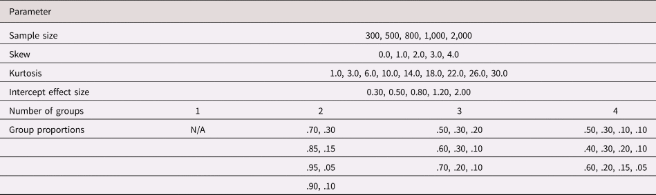
Numbers of groups were predetermined, ranging from k = 1–4 (see Table 1). Group means were varied based on intercept effect sizes. Group separation was evaluated by manipulating noncentered intercept effect sizes (Cohen's d) from small to large (0.30–2.00).Footnote 4 Proportions of observations in each group were varied to mimic developmental and psychopathology data. In developmental research, trajectory classes are often of relatively equal proportions, such as those seen in self-regulation (e.g., Montroy, Bowles, Skibbe, McClelland, & Morrison, Reference Montroy, Bowles, Skibbe, McClelland and Morrison2016). In psychopathology research, relative rarity of a trait in the population is typically a defining feature (e.g., Kotov et al., Reference Kotov, Krueger, Watson, Achenbach, Althoff, Bagby and Wright2017). We therefore modeled both.
Summary of parameters varied across 1,955,000 simulations

Note: All combinations of parameters were evaluated across 1,000 replications.
Ten combinations of subgroup proportions were modeled (see Table 1). For the one-group analyses, skew and kurtosis were manipulated to evaluate effects of nonnormality. Skew ranged from none to extreme (0.0–4.0). Kurtosis ranged from leptokurtic to extremely platykurtic (1.0–26.0). Given that skew and kurtosis are dependent, kurtosis was necessarily large when skew was large (see Table 1). This approach is similar to that reported by Bauer and Curran (Reference Bauer and Curran2003a). For two- to four-group data, skew and kurtosis were not manipulated directly because mixing subgroups imparts skew and kurtosis. Normally distributed residual error was added to each data point (cf. Serang et al., Reference Serang, Zhang, Helm, Steele and Grimm2015). We simulated 1,955 unique parameter combinations, each of which was replicated 1,000 times, consistent with previous research (Peugh & Fan, 2015).
Four quadratic growth and exponential growth patterns were simulated. Quadratic growth included both U-shaped and inverted U-shaped patterns. Large inverted quadratic growth was defined as f(x) = −2x 2 + 12x + c. Small inverted U-shaped quadratic growth was defined as f(x) = −0.5x 2 + 3x + c, where c depended on the effect size between the groups and the location of the curve. For example, for large inverted quadratic growth at Time 1 (T1) where T = 50, f(x) = −2x 2 + 12x + 40, but when T1 had a value of 55 the equation was f(x) = −2x 2 + 12x + 45 (see supplementary materials A, Figures S1–S6, for examples). Similarly, U-shaped growth was defined as f(x) = 0.5x 2 − 3x + c. Exponential patterns differed given little growth from T1 to T2, but increasingly rapid growth thereafter. For large exponential patterns, growth was defined as f(x) = T1 value + 2.0x where x = 1, 3, 6. For small exponential patterns, growth was defined as f(x) = T1 value + 0.25(x) where x = 1, 3, 6. For decreasing patterns, exponential growth terms were negative.Footnote 5 Trajectories are plotted in the online supplementary materials, Figures S1–S6.
We used R (R Core Team, 2013) to simulate data, which were then analyzed using MplusAutomation in R (Hallquist & Wiley, Reference Hallquist and Wiley2018; Muthén & Muthén, Reference Muthén and Muthén2015). Descriptives for each analysis were exported to Microsoft® Excel. Means, SDs, ranges, and GMM results, including multiple fit statistics, were saved. Given their common use in the literature (Bauer & Curran, Reference Bauer and Curran2003a; Bozdogan, Reference Bozdogan1987; Jung & Wickrama, Reference Jung and Wickrama2008; Nagin, Reference Nagin1999), we compare AIC, BIC, LMR, and BLRT in evaluating model fit. We also report the normalized entropy criterion (Celeux & Soromenho, Reference Celeux and Soromenho1996; Biernacki & Govaert, Reference Biernacki and Govaert1999). For purposes of this study, we evaluate “success” in two ways. First, we report accuracy of each individual fit statistic, as well as entropy, in identifying the correct number of groups. For entropy, which is typically not considered as a fit index but is nevertheless used to evaluate classification quality (see above), values closest to 1.0 were assumed to indicate best fit. In addition, because decisions about fit are usually reached based on multiple fit indices, we also evaluate success based on whether a simple majority of “fit” statistics (three out of five including AIC, BIC, LMR, BLRT, and entropy) identified the true number of groups. No index was weighted more heavily than others. Of note, our use of the term “success” applies only to solutions that converged and indicated the correct number of groups based on these decision rules. We consider failure to converge to be a separate, less critical issue, because such failures are not likely to be interpreted as supporting any grouping solution. We refer readers elsewhere for further discussion (e.g., Grimm et al., Reference Grimm, Ram, Shiyko, Lo, McArdle and Ritschard2014).
One-group simulations
Nonnormal distributions were created using SimMultiCorrData in R (see online supplementary material B for R code; Fialkowski, Reference Fialkowski2018) for samples sizes of N = 300, 500, 800, 1,000, and 2,000. The Fleishman power method was selected for simulations, which allows kurtosis to be greater than or equal to skew squared, minus 2.0 (Fleishman, Reference Fleishman1978). Skew and kurtosis were combined as follows: skew 0.0 or 1.0 with kurtosis 1.0, 3.0, or 6.0; skew 2.0 with kurtosis 6.0, or 14.0; skew 3.0 with kurtosis 14.0; and skew 4.0 with kurtosis 26.0. This provides a range of distributions from normal (skew = 0.0, kurtosis = 3.0) to extremely skewed and platykurtic (skew = 4.0, kurtosis = 26.0). Linear growth was varied from none (slope = 0.0), small increase (slope = 0.5), large positive increase (slope = 2.0), and medium decrease (slope = −1.0). Larger slopes may provide more favorable conditions for groups to be identified. For nonlinear growth, one curve was simulated as quadratic and inverted U-shaped, and two were simulated with exponential (see online supplementary material A, Figure S1).
Two-group simulations
For all k > 1 simulations, effect sizes (d) separating distributions were specified in terms of uncentered intercepts. Four simulations had linear growth, one had quadratic growth, and one had exponential growth (online supplementary material A, Figure S2). The same linear growth patterns were used for two groups as for one group (see above). For quadratic growth and exponential growth, several patterns were combined across different simulations (e.g., no growth/large bell shape; small exponential decrease/large exponential increase).
Three-group simulations
For the three-group simulations, uncentered intercept effect sizes (d) were set between Group 1 and Group 2 and Group 1 and Group 3. Seven combinations of effect size were used (0.3/0.5, 0.3/0.8, 0.3/1.2, 0.3/2.0, 0.5/0.8, 0.5/1.2, 0.5/2.0). Four linear growth patterns, one quadratic growth pattern, and one exponential growth pattern were simulated (online supplementary material A, Figures S3–S4). Linear models included (a) no growth for all groups; (b) no growth for Groups 1 and 3, small increase for Group 2 (slope = 0.5); (c) no growth for Group 1, large increase for Group 2 (slope = 2.0) and small decrease of Group 3 (slope = −0.5); and (d) small decrease for Group 1 (slope = −0.5), no growth for Group 2, and large growth for Group 3 (slope = 2.0). The quadratic growth pattern included no growth for Group 1, small U-shaped growth forGroup 2, and small inverted U-shaped growth for Group 3. The exponential growth pattern included a small decrease for Group 1, small increase for Group 2, and a large increase for Group 3 (see previous definitions of growth; supplementary material A, Figure S4).
Four-group simulations
For the four-group simulations, uncentered intercept effect sizes (d) were set between Group 1 and Group 2, Group 1 and Group 3, and Group 1 and Group 4. Five combinations of effect size were used (0.3/0.5/0.8, 0.3/0.5/1.2, 0.3/0.5/2.0, 0.3/0.8/1.20, 0.3/0.8/2.0). Four linear growth patterns (online supplementary material A, Figure S5), one quadratic growth pattern, and one that included an exponential growth pattern and a quadratic growth pattern were simulated (online supplementary material A, Figure S6). For both types of simulations data “crossed-over,” creating an “X” pattern. Similar patterns have been reported repeatedly in the externalizing literature (e.g., Arnold et al., Reference Arnold, Ganocy, Mount, Youngstrom, Frazier, Fristad and Marsh2014; Odgers et al., Reference Odgers, Moffitt, Broadbent, Dickson, Hancox, Harrington and Caspi2008). Linear models included: (a) no growth for all groups; (b) no growth for Groups 1 and 4, small increase for Group 2 (slope = 0.5), and small decrease for Group 3 (slope = −0.5); (c) no growth for Groups 1 and 4, large increase for Group 2 (slope = 2.0), and large decrease for Group 3 (slope = −2.0); and (d) no growth for Group 1, small decrease for Group 2 (slope = −0.5), increase for Group 3 (slope = 1.0), and large growth for Group 4 (slope = 2.0). The quadratic growth pattern included no growth for Groups 1 and 4, small U-shaped growth for Group 2, small inverted U-shaped growth for Group 3, and large inverted U-shaped growth for Group 4. The exponential/quadratic growth pattern included small U-shaped growth for Group 1, small decrease for Group 2 (T1 − .25x where x = 1,3,6), large increase for Group 3 (T1 + 2.0x where x = 1, 3, 6), and small inverted U-shaped growth for Group 4.
Mplus
Mplus 8.0 (Muthén & Muthén, Reference Muthén and Muthén2015) was used for all analyses. We used basic syntax with minor alterations. GMMs were estimated using maximum likelihood with robust standard errors, with expectation-maximization implemented (Muthén & Muthén, Reference Muthén and Muthén2015). Expectation-maximization allows the unobserved group classification variable to be treated as a latent variable (Ram & Grimm, Reference Ram and Grimm2009). In order to maximize the likelihood of the data given model parameters, an iterative procedure is used to obtain parameter estimates and posterior estimates of each observation's class membership probability. Example Mplus code appears in online supplementary material B.
Results
All simulations were run in a large computer laboratory over the course of 4.5 months on 35 identical personal computer workstations with Intel® Core™ i3-3220 processors (3.30 GHz).
One-group simulations
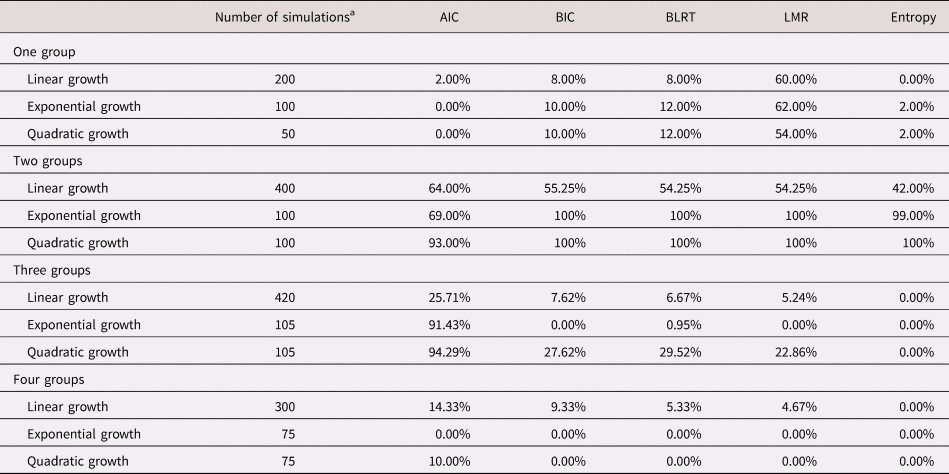
Results are summarized in online supplementary material A, Tables 3–5. Online supplementary material Figure S7 depicts a graphical example of output. Four linear models were simulated, including: (a) linear no growth (slope = 0.0); (b) linear growth with a decrease (slope = −1.0); (c) linear growth with a large increase (slope = 2.0); and (d) linear growth with a small increase (slope = 0.5). Fit indices often disagreed, with one to five groups being identified. For most models (88%), only two to three fit indices agreed and for some models (3.5%), all fit indices suggested different solutions. LMR was most successful, identifying one group as the best fit more than all other fit indices (60%), whereas AIC (2.0%), BIC (8.0%), BLRT (8.0%), and entropy (0.0%) were largely unsuccessful (see Table 2).
Percentage of correctly identified groups for each fit statistic and entropy

a All values represent simulation aggregates with 1,000 replications each.
AIC = Akaike information criterion; BIC = Bayesian information criteria; BLRT = bootstrap parametric likelihood ratio test; LMR = Lo–Mendell–Rubin likelihood ratio test.
No growth
In the no growth simulations GMM was largely unsuccessful (online supplementary material A, Tables 3 and 5). Across all 50 parameter combinations, only four (8.0%) of aggregates (averages across all 1,000 replications) correctly identified one group. Most models identified two to five groups. GMM was successful primarily when skew was 0.0 and kurtosis was 1.0, as in previous research (see above). In such cases, multiple fit indices (at least three) supported one group when sample sizes were 300, 500, 800, and 1,000. Of note, the larger the sample size the less successful entropy, AIC, BLRT, and LMR were in identifying the correct number of groups. However, BIC was fairly consistent across sample sizes. Online supplementary material A, Table 5 provides percentages of the 1,000 replications for which each fit index correctly identified one group. For other skew and kurtosis combinations, one group was rarely identified because fit indices disagreed. However, LMR often identified one group for sample sizes 300–1,000. However, LMR was less successful for sample size 2,000.
Linear decreasing growth
Given decreasing linear growth, GMM was largely unsuccessful (online supplementary material A, Tables 3 and 5). Across all 50 parameter combinations, only three (6.0%) aggregates correctly identified one group. For skew of 0.0 and kurtosis of 1.0, GMM was partly successful for sample sizes of 300, 500, and 1,000; at least three fit indices identified one group. For other skew and kurtosis combinations, LMR was most successful at identifying one group. Entropy often suggested two groups, whereas fit indices (AIC, BIC, BLRT) identified a range of groups, often four or five.
Gradual linear increasing growth
For gradual linear growth, GMM was largely unsuccessful (online supplementary material A, Tables 3 and 5). Across all 50 parameter combinations, only three (6.0%) aggregates correctly identified one group. One group was identified when skew was 0.0 and kurtosis 1.0 for sample sizes 300, 500, and 1,000. For the remaining skew and kurtosis combinations, fit indices often disagreed, with two to five groups identified.
Steep linear increasing growth
Given steep linear growth, GMM was largely unsuccessful in identifying one group (online supplementary material A, Tables 3 and 5). Across all 50 parameter combinations, only four (8.0%) aggregates correctly identified one group. For sample sizes 300, 500, 800, and 1,000, when skew was 0.0 and kurtosis was 1.0, three fit indices identified one group (BIC, BLRT, LMR). Again, fit indices were often less successful with larger samples. For remaining skew and kurtosis combinations, fit indices largely disagreed, suggesting two to five groups. Consistent with the other linear simulations, LMR identified one group fairly consistently, but identified more groups when the sample size was 2,000.
Exponential growth
Two exponential growth patterns were simulated, one with gradual growth and one with steep growth. For both patterns, GMM was largely unsuccessful (online supplementary material A, Tables 4 and 5). Across all 50 parameter combinations, only 10 (10%) aggregates were successful. For skew of 0.0 and kurtosis of 1.0, with sample sizes 300, 500, 800, and 1,000; and for sample size 300, skew of 0.0 and kurtosis of 3.0, three fit indices (BIC, BLRT, LMR) identified one group. For successful analyses, BIC performed best, with 74% to 100% of successful identifications of one group across individual replications. However, LMR performed best for aggregates, successfully identifying one group in 62 of 100 simulations (see Table 2 for summary). Entropy and AIC identified at least two groups and as many as five. For the remaining skew and kurtosis combinations, more than one group was identified, and fit indices often disagreed.
Quadratic inverted U-shaped growth
For U-shaped growth, GMM was largely unsuccessful in identifying one group (online supplementary material A, Tables 4 and 5). Across all 50 parameter combinations, only five (10%) aggregates were successful. LMR was the most successful (54.0%), whereas AIC (0.0%), BIC (10.0%), BLRT (12.0%), and entropy (2.0%) were largely unsuccessful (see Table 2). For skew of 0.0 and kurtosis 1.0, samples sizes 300, 500, 800, and 1,000, three fit indices identified one group. For skew of 0.0, kurtosis of 3.0, and sample size 300, three fit indices identified one group. For the remaining skew and kurtosis combinations, two to five groups were identified.
Two-group simulations
Results are summarized in online supplementary A, material Tables 6–10. Online supplementary material, Figure S8 provides graphical examples. Four linear growth patterns were simulated. Overall, patterns with one to three groups were identified for best fit, with most models identifying one or two groups. GMM was most successful with large sample sizes and large intercept effect sizes. However, with one low base-rate group (.95/.05) – a common state of affairs in psychopathology research – GMM often identified one group instead of two. Fit indices varied considerably in performance. Across all 400 parameter combinations (100 per growth pattern), measures of fit performed as follows: AIC 64.0%, BIC 55.25%, BLRT and LMR 54.25%, and entropy 42.0% (see Table 2). Thus, entropy was less sensitive than fit indices in identifying one group versus two groups.
No growth
When both groups had no growth, GMM was unsuccessful when effect sizes were anything but very large, consistent with previous research (see above). When effect size was <2.0, GMM correctly identified two groups in only nine of 100 aggregates (online supplementary material A, Tables 6 and 7). For effect sizes of 0.3, 0.5, 0.8, and 1.2, one group was identified consistently for all sample sizes and group proportions by most fit indices. The best performing fit statistic was AIC, which correctly identified two groups for 27% of aggregates. When proportions were .95 and .05, one group was identified by all fit indices for effects sizes smaller than 2.0. GMM was more effective when the intercept effect size was 2.0, especially with large sample sizes. For sample sizes 800 and 1,000, AIC, BIC, BLRT, and LMR correctly identified two groups for proportions .70/.30, .85/.15, and .90/.10, whereas entropy consistently identified one group. For proportion .95/.05, AIC identified two groups when effect size was 2.0, whereas other measures of fit identified two groups only for large sample sizes. For sample size 2,000, two groups were identified by AIC, BIC, BLRT, and LMR for all proportions.
Gradual linear growth
GMM was largely unsuccessful with one low and stable group and one gradually increasing group (slope = 0.5). Correct results were obtained in only 16 of 100 aggregated simulations (online supplementary material A, Tables 6 and 7). For effect sizes 0.3 and 0.5, GMM identified one group for all sample size and proportion combinations. When effect size was 0.8, one group was identified for sample sizes 300, 500, and 800 for all proportions. For sample size 800 there was one exception: AIC identified two groups for proportion .85/.15. For sample sizes 1,000 and 2,000 and proportions .70/.30, .85/.15, and .90/.10, AIC also identified two groups. GMM was more successful identifying two groups when effect size was 2.0. When sample size was 500, two groups were identified for proportions .70/.30, .85/.15, and .90/.10, but not for .95/.05. For samples sizes 800, 1,000, and 2,000, two groups were identified for all proportions. For sample size 2,000 and effect size 1.2, two groups were identified for proportions .85/.15.
Steep linear growth
GMM was quite successful with one low and stable group and one steeply increasing group (slope = 2.0), Under such conditions, two groups were identified for all combinations of sample size, proportions, and effect size (online supplementary material A, Table 8). Fit indices and entropy were equally successful across aggregates of the 1,000 parameter combinations, with AIC, BIC, BLRT, and LMR identifying two groups and entropy agreeing. For each replication, however, measures of fit performed differently: AIC 50.10–66.90%, BIC 86.5–100%, BLRT 87.9–98.3%, LMR 80.50–89.80%, and entropy 57.6–96%.
Gradual and steep linear growth
GMM was largely successful with one gradually increasing and one steeply increasing group. In this situation, GMM correctly identified two groups across 91 of 100 simulation aggregates (online supplementary material A, Table 9). Failures to identify two groups occurred with smaller sample sizes (≤ 500), small to medium effect sizes (≤ 0.8), and low base rates (.95/.05). Success across the 1,000 replications ranged considerably by fit index: AIC 36.5–66.10%, BIC 22.0–100%, BLRT 32.6–97.9%, and LMR 40.0–89.9%. Entropy was more variable, 0.0–83.6%. As in other simulations described above, BIC, BLRT, and LMR performed poorly when the base rate was low (95/.05), whereas AIC performed equally well across proportions (online supplementary material A, Table 10).
Exponential growth
Exponential growth results are summarized in online supplementary material A, Table 11. Example graphs appear in supplementary material, Figure S9. Given steep exponential growth, most fit indices successfully identified two groups across simulation aggregates, with the exception of AIC, which sometimes identified three. Across the 1,000 replications, fit indices performed as follows: AIC 32.30–45.50%, BIC 98.90–100.00%, BLRT 90.50–98.40%, LMR 74.80–86.80%. Entropy performed between 0.90 and 70.90%.
Quadratic inverted U-shaped growth
Results are summarized in online supplementary material A, Table 12, with example graphs appearing in Figure S9. For inverted U-shaped growth, GMM successfully identified two groups 100% of the time. Aggregated across parameter combinations, fit indices performed comparably, ranging from 93.0% (AIC) to 100% (BIC, BLRT). Across the 1,000 replications, fit indices performed as follows: AIC 37.20–55.00%, BIC 99.5–100%, BLRT 91.80–97.80%, LMR 74.70–84.70%. Entropy performed between 77.40 and 91.20%.
Three-group simulations
Results for the three-group simulations are summarized in online supplementary material A, Tables 13–15 and Figure S10. In general, GMM was ineffective in the linear, three-group simulations. For most of these simulations, GMM identified one to two groups. Across 420 aggregated simulations, GMM identified three groups only 6.67% of the time. The only exception occurred when there was one increasing, one stable, and one decreasing group. Even then, GMM was successful in only 26.67% of 105 aggregated simulations. In comparing fit indices, three groups were identified as follows: AIC 25.71%, BIC 7.62%, BLRT 6.67%, LMR 5.24%, and entropy 0.00% (see Table 2).
No growth
When all three groups had stable growth, GMM was largely unsuccessful (online supplementary material A, Table 13). For the 105 simulation aggregates, one group was incorrectly identified in most cases: AIC 67.62%, BIC 92.38%, BLRT 88.57%, and LMR 90.48%. Entropy never suggested three groups. In most other cases, two groups were identified incorrectly: AIC 32.38%, BIC 7.62%, BLRT 11.43%, and LMR 9.52%. Entropy never suggested two groups.
Linear growth with gradual increase for one group
When two groups were stable and one had gradually increasing growth (slope = 0.5), GMM was largely unsuccessful in identifying three groups (online supplementary material A, Table 13). For the 105 simulation aggregates, one group was incorrectly favored by all fit indices: AIC 65.71%, BIC 94.29%, BLRT 90.48%, and LMR 91.43%. Entropy suggested one group 100% of the time. Two groups were also identified incorrectly, but less often: AIC 27.62%, BIC 5.71%, BLRT 9.52%, and LMR 8.57%. Entropy never suggested two groups. Only AIC identified three groups, and only in 6.67% of simulation aggregates.
Linear growth with no increase for one group, steep increase for one group, and gradual decrease for one group
In this situation, GMM was marginally successful at best (online supplementary material A, Tables 14 and 15). For results across 105 simulation aggregates, performance in identifying three groups was as follows: AIC 87.62%, BIC 30.48%, BLRT 26.67%, and LMR 20.95%. Entropy never suggested three groups. As noted above, even though AIC performed fairly well, failure of multiple fit indices to agree can be considered as nonsuccess. Using fit index agreement as a criterion, three groups were identified in very circumscribed situations, including (a) effect size combinations of 0.3/2.0 (with the first group as reference; see above) and 0.5/2.0 (for other effect size combinations, two groups were identified); (b) a sample size of 300, with effect size combinations of 0.3/2.0 and 0.5/2.0 and subgroup proportions of .50/.30/.20; and (c) a sample size of 2,000, an effect size of 0.3/1.2 and subgroup proportions of .50/.30/.20. Within replications, fit indices performed as follows: AIC 60.20–69.90%, BIC 60.30–100.0%, BLRT 82.40–97.10%, and LMR 59.40–87.50%. Entropy suggested three groups between 0 and 5.30% of the time.
Linear growth with gradual decrease for Group 1 and steep increase for Group 3
For this pattern, groups differed in growth but did not overlap (like the two patterns described above), potentially making these groups easier to identify. In this scenario, GMM was largely unsuccessful (see online supplementary material A, Table 14). Fit indices consistently identified two groups. BIC, BLRT, and LMR identified two groups for 105 (100%) of the simulation aggregates. Entropy suggested two groups 100% of the time as well. AIC was only slightly successful, identifying three groups for nine (8.57%) of the 105 simulation aggregates, and two groups for the remaining 96 (91.43%).
Exponential growth simulation
Results for exponential growth appear in online supplementary material A, Table 16. A graphical example is depicted in supplementary material, Figure S11. With gradual decrease for Group 1, gradual increase for Group 2, and steep growth for Group 3, BIC and LMR incorrectly identified two groups in 100% of simulation aggregates, with BLRT following close behind at 99.05%. Entropy suggested two groups 100% of the time. In contrast, AIC was mostly successful, identifying three groups for 96 of the 105 simulation aggregates. In 8.57% of simulations, AIC identified four groups, but was the only fit index to do so.
Quadratic inverted U-shaped growth
Results for inverted U-shaped growth are summarized in online supplementary material A, Tables 16 and 17, with a graphical example in supplementary material, Figure S11. Findings were again marginal at best. Across the 105 simulation aggregates, performance in identifying three groups was as follows: AIC 94.29%, BIC 27.62%, BLRT 29.52%, and LMR 22.86%. Entropy never suggested three groups. Using fit index agreement as a criterion, three groups were identified in the following circumscribed situations: (a) when sample size was 300, effect sizes were 0.3/2.0, and subgroups proportions were .50/.30/.20; (b) when sample sizes were 500, 800, 1,000, and 2,000 and effect sizes were 0.3/2.0 and 0.5/2.0; and (c) when sample size was 2,000, subgroup proportions were .50/.30/.20, and effect sizes were 0.3/1.2 and 0.5/1.2. Across all 105 simulation aggregates 25.71% were successful according to index agreement. When considering the 1,000 replications, fit indices performed as follows: AIC 47.90–57.60%, BIC 50.40–100.00%, BLRT 77.10–92.90%, and LMR 57.70–82.10%. Entropy suggested three groups 0.0–5.20% of the time.
Four-group simulations
Results for four-group simulations are summarized in online supplementary material A, Tables 18–20. Graphical examples appear in supplementary material, Figure S12. Four separate linear growth models were simulated, as described below. Across 300 aggregated simulations, GMM identified four groups only 5.0% of the time. Four groups were identified as follows: AIC 14.33%, BIC 9.33%, BLRT 5.33%, LMR 4.67%, and entropy 0.00% (see Table 2).
No growth
GMM was unsuccessful when all subgroups showed no growth (online supplementary material A, Table 18). Out of 75 simulation aggregates, 71 identified one group and four identified two groups. Thus, regardless of intercept effect combination (0.3/0.5/0.8, 0.3/0.5/1.2, 0.3/0.5/2.0, 0.3/0.8/1.20, 0.3/0.8/2.0 with the first group as reference; see above), one-group solutions predominated as follows: AIC 60.0%, BIC 96.0%, BLRT 94.67%, and LMR 94.67%. Entropy always suggested one group. None index suggested more than two groups.
Gradual linear growth with crossover
This growth pattern included flat growth for two groups, gradually increasing growth for one group (slope = 0.5), and gradually decreasing growth for one group (slope = −0.5). Results are summarized in online supplementary material A, Table 19. As in the no growth simulations described immediately above, 71 of the 75 aggregates identified one group as follows: AIC 54.67%, BIC 96.0%, BLRT 93.33%, and LMR (96.0%). Entropy suggested one group 100% of the time. AIC occasionally identified three groups, but no fit index ever identified four.
Steep linear growth with crossover
This pattern included flat growth for two groups, steep positive growth for one group (slope = 2.0), and steep negative growth for one group (slope = −2.0). In this situation GMM was more effective, yet still performed poorly. Of 75 simulation aggregates, 20.0% identified four groups. For sample size 300, between one and three groups were identified. Four groups were correctly identified by at least three measures of fit and/or entropy for the following: (a) sample size 500, effect sizes 0.3/0.8/2.0, and group proportions .40/.30/.20/.10; (b) samples sizes 800, 1,000, and 2,000, when one effect size was 2.0 and the largest proportion was .40 or .50; and (c) sample size 2,000, when the largest proportion was .60 (online supplementary material A, Table 18).
Overall, entropy suggested one (60.0%) or three (40.0%) groups. In contrast, fit indices were somewhat successful. AIC identified four groups for 36 (48.0%), BIC for 28 (37.33%), BLRT for 16 (21.33%), and LMR for 14 (18.67%) of the 75 aggregates. When considering replications for the successful aggregates, entropy suggested four groups for 0 (0%), AIC for 654 to 721 (65.40%–72.10%), BIC for 612 to 1,000 (61.20%–100.0%), BLRT for 812 to 965 (81.20%–96.50%), and LMR 676 to 838 (67.60%–83.80%) of the 1,000 replicates (see online supplementary material A, Table 20).
Fan-shaped linear growth
This growth pattern included no growth for Group 1, small decrease for Group 2 (slope = −0.5), increase for Group 3 (slope = 1.0), and large growth for Group 4 (slope = 2.0). Here, 74 (98.68%) of the aggregated models identified two groups, one model identified three groups, and occasionally (9.33%) AIC identified four groups. Entropy consistently suggested one (26.67%) or two (73.33%) groups. Two groups were favored by BIC (98.67%), BLRT (97.33%), and LMR (97.33%). AIC was mostly split between two (44.0%) and three (46.67%) groups. Generally, fit indices agreed on group numbers. However, there were simulations where the fit statistics differed. For sample sizes of 2,000, there was more disagreement than for smaller sample sizes (see online supplementary material A, Table 19 for results).
Exponential/quadratic growth
Results are summarized in online supplementary material A, Table 21. The exponential/quadratic growth pattern included small U-shaped growth for Group 1, small exponential decrease for Group 2, large exponential increase for Group 3, and small inverted U-shaped growth for Group 4. GMM was unsuccessful, one group was identified as best fit for 72 of the 75 simulation aggregates. Occasionally, AIC identified two (18.67%) or three (30.67%) groups. Entropy (100%), BIC (98.67%), BLRT (96.0%), and LMR (96.0%) favored one group. No fit indices or entropy identified four groups.
Quadratic inverted U-shaped growth
Results are summarized in online supplementary material A, Table 21. The quadratic growth pattern included no growth for Groups 1 and 4, small U-shaped growth for Group 2, small inverted U-shaped growth for Group 3, and large inverted U-shaped growth for Group 4. GMM was unsuccessful in identifying four groups. Fit indices and entropy were inconsistent. AIC was the only fit index to correctly identify four groups (10%, see Table 2). AIC identified three groups for the remaining 45 aggregates. Entropy (two groups = 73, three groups = 2), BIC (two groups = 55, three groups = 20), BLRT (two groups = 57, three groups = 14), and LMR (two groups = 67, three groups = 8) all suggested two to three groups.
Discussion
Psychologists have long attempted to identify homogeneous subgroups of individuals within larger samples using statistical methods. Such methods often become popular and are used heavily until limitations are discovered and new methods are created. GMM is a contemporary method designed to identify latent trajectory classes based on longitudinal growth data. In the last decade, GMM has been used to identify groups in a variety of fields (Peugh & Fan, Reference Peugh and Fan2012). As reviewed in the introduction of this article, GMM is especially popular in psychopathology research. This includes research on depression (Jinnin et al., Reference Jinnin, Okamoto, Takagaki, Nishiyama, Yamamura, Okamoto and Yamawaki2016), anxiety (e.g., Spinhoven et al., Reference Spinhoven, Batelaan, Rhebergen, van Balkom, Schoevers and Penninx2016), posttraumatic stress disorder (e.g., Allan et al., Reference Allan, Gros, Myers, Korte and Acierno2017), substance use (Passarotti et al., Reference Passarotti, Crane, Hedeker and Mermelstein2015), attention problems (e.g., Arnold et al., Reference Arnold, Ganocy, Mount, Youngstrom, Frazier, Fristad and Marsh2014), callous–unemotional traits (e.g., Fontaine et al., Reference Fontaine, McCrory, Boivin, Moffitt and Viding2011), antisocial behavior (e.g., Connell & Frye, Reference Connell and Frye2006; Odgers et al., Reference Odgers, Moffitt, Broadbent, Dickson, Hancox, Harrington and Caspi2008), suicide attempts (e.g., Nkansah-Amankra, Reference Nkansah-Amankra2013), relationship violence (Brooks-Russell et al., Reference Brooks-Russell, Foshee and Ennett2013), personality disorders (Hallquist & Lenzenweger, Reference Hallquist and Lenzenweger2013), and more.
Much of this research treats identified latent trajectory classes as different in kind (discrete), even though previous research shows that GMM sometimes over-extracts latent classes from dimensionally distributed data (Bauer & Curran, Reference Bauer and Curran2003a; Depaoli et al., Reference Depaoli, Winter, Lai and Guerra-Peña2019; Grimm et al., Reference Grimm, Ram, Shiyko, Lo, McArdle and Ritschard2014; Hoeksma & Kelderman, Reference Hoeksma and Kelderman2006). This can be problematic because (a) latent classes tend to get reified in the literature, and (b) polychotomizing continua often results in lower statistical power and can even yield misleading inferential statistics (MacCallum, Zhang, Preacher, & Rucker, Reference MacCallum, Zhang, Preacher and Rucker2002). For these reasons and others, some have argued that GMM should be used primarily for exploratory purposes (Ram & Grimm, Reference Ram and Grimm2009).
Although a number of Monte Carlo studies have assessed GMM performance across a range of distribution parameters (e.g., Bauer & Curran, Reference Bauer and Curran2003a; Chen et al., Reference Chen, Kwok, Luo and Willson2010; Depaoli, Reference Depaoli2013; Depaoli et al., Reference Depaoli, Yang and Felt2017, Reference Depaoli, Winter, Lai and Guerra-Peña2019; Grimm et al., Reference Grimm, Ram, Shiyko, Lo, McArdle and Ritschard2014; Guerra-Peña et al., Reference Guerra-Peña, García-Batista, Depaoli and Garrido2020; Hoeksma & Kelderman, Reference Hoeksma and Kelderman2006; Muthén & Asparouhov, Reference Muthén and Asparouhov2015; Peugh & Fan, Reference Peugh and Fan2012), our work extends these findings to include more simulations, more time points, and larger samples, which are increasingly common in latent trajectory modeling. Findings are consistent with previous work indicating over-extraction of latent classes with nonnormal data, disagreement among fit statistics regarding the correct number of classes, and very large effect sizes required to resolve latent group structure. Importantly, our findings also demonstrate that incorrect numbers of classes are often identified across fit statistics, which has clear implications for misrepresenting data structure, and for characterizing individual's trajectories of important behaviors. This calls into question the use of GMM in strictly bottom-up, atheoretical contexts. As noted above, Bayesian approaches to GMM hold promise in this regard given theoretically informed priors (e.g., Depaoli et al., Reference Depaoli, Yang and Felt2017; Serang et al., Reference Serang, Zhang, Helm, Steele and Grimm2015). Further research on Bayesian approaches is therefore warranted. Collectively, our results suggest more caution when using and interpreting standard GMM. Below we summarize our findings in more detail.
Nonnormal distributions
One-group simulations included manipulation of skew and kurtosis. GMM performed best when skew and kurtosis were minimal. In contrast, when skew and/or kurtosis increased, GMM over-extracted latent classes, consistent with previous research (Bauer & Curran, Reference Bauer and Curran2003a; Grimm et al., Reference Grimm, Ram, Shiyko, Lo, McArdle and Ritschard2014). In addition, for most one-group simulations, fit indices disagreed, making it difficult to select a best model. Entropy consistently identified two groups, whereas fit indices identified one to five groups. For the one-group simulations, fit indices identified five groups more often than they did for any other simulation condition (i.e., two, three, and four groups). The only exception was LMR. This suggests that under conditions that are common in psychopathology research, GMM may impose structure rather than identifying existing latent subgroups. These findings suggest that recent efforts to develop GMM in ways that reduce effects of nonnormality, such as those using skew t family distributions (Guerra-Peña et al., Reference Guerra-Peña, García-Batista, Depaoli and Garrido2020; Muthén & Asparouhov, Reference Muthén and Asparouhov2015), should continue.
Intercept effect size
For the k = 2–4 group simulations, GMM unsurprisingly performed better with less group overlap. For the two-group simulations, intercept effect size was less influential than growth over time. This was especially so for steep growth, where GMM performed well. For gradual growth, intercept effect size was more important. When there were three or four groups, simulations that included an effect size of 2.0 performed somewhat better. However, as online supplementary material A, Tables 13–21 show, this was not fully consistent. Although unsurprising, such findings are problematic given that effect sizes in psychology are usually small to modest (e.g., Cohen, Reference Cohen1988). Here again, our findings suggest caution in interpreting outcomes from GMM, and suggest that recently articulated Bayesian methods may be helpful (Depaoli et al., Reference Depaoli, Yang and Felt2017; Serang et al., Reference Serang, Zhang, Helm, Steele and Grimm2015).
Proportions
For the two-group simulations, GMM was most effective when relative proportions for each group were close to even. GMM was ineffective with especially low group proportions (.95/.05), and was only slightly more effective for .70/.30 and .85/.15 proportions. When there were three to four groups, GMM also performed poorly when one group was small compared to others (.60/.30/.10, .60/.20/.15/.05, etc.). Poor performance with low base-rate classes is likely to be a function of those classes having limited effect on altering normality. As others have noted, GMM is most effective at recovering groups when they impart appreciable skew and kurtosis into mixed distributions. This is likely to require more “tail weight” than, for example, the .05 contribution to a .95/.05 mixing proportion provides (see also Bauer & Curran, Reference Bauer and Curran2003a; Grimm et al., Reference Grimm, Ram, Shiyko, Lo, McArdle and Ritschard2014). Of note, however, sample size also affected results. For large samples, GMM performed better when proportions were unequal. Although more research is needed to clarify the role of group proportions in the accuracy of GMM, it seems safe to say that when one group is particularly small, results are compromised unless sample size is especially large.
Sample size
Following from what is discussed immediately above, and consistent with past research, GMM performed best with large samples (Connell & Frye, Reference Connell and Frye2006). Of note, however, empirical instantiations of GMM often use sample sizes that yielded mixed results in our simulations. Psychopathology research is often conducted with samples of a few hundred participants. When sample size was 300 – the smallest we simulated – GMM was ineffective across a wide range of parameter combinations. Thus, use of GMM may be better reserved for very large data sets. This is especially important when more than two groups are hypothesized, as GMM had particular difficulty in identifying three or four groups with anything but large samples.
Fit indices
Although comparing fit indices was a secondary aim, several findings emerged. When one group was simulated, AIC, BIC, and BLRT consistently identified three to five groups, and entropy often identified two groups. LMR was much more effective in identifying one group. When two groups were simulated, entropy often identified one group even when other fit indices correctly identified two groups. When three groups were simulated, all fit indices identified one to two groups for the majority of aggregated results. However, when linear growth was steep for Group 2 and gradually decreased for Group 3, AIC performed better than all other fit indices, identifying three groups in almost 90% of the aggregated results. Interestingly, however, when individual replications were considered, BIC and BLRT performed better than AIC. Furthermore, entropy identified fewer than three groups for every aggregated result and for most replications. When four groups were simulated and GMM was successful, entropy suggested one to two groups even when other fit indices identified four. In reviewing replications, BIC and BLRT performed best, with AIC often identifying five groups and LMR often identifying three or fewer.
Overall, BIC and BLRT performed better with more groups. AIC often identified too many groups and entropy too few. When there were two groups, all indices but entropy performed better. It is important to note that (a) fit indices usually disagreed, and in many cases only one (and in some cases none) identified the correct number of groups; and (b) because the true number of groups is unknown and unobservable in practice and no fit index performs uniformly better than others, it is not possible to make recommendations for which fit index to “trust.” For example, although LMR was most successful with one group and AIC was most successful with four, most simulations with only one group suggested between two and five groups based on model fit. Given these findings, it might be tempting to rely on AIC if four groups are suggested, but doing so is logically dubious because, despite performing best, AIC was correct only 14.3% of the time. Choosing four-group solutions based on AIC would therefore yield incorrect conclusions far more often than not, even though it performs better than all other fit indices. Many other examples could be provided. The bottom line is that one cannot accurately determine the correct number of groups in practice, and no identifiable combination of indicators improves performance appreciably.
Implications
Results discussed herein may have implications for a broad range of research using GMM. In the psychopathology literature, many if not most studies identify three to four groups (e.g., Arnold et al., Reference Arnold, Ganocy, Mount, Youngstrom, Frazier, Fristad and Marsh2014; Odgers et al., Reference Odgers, Moffitt, Broadbent, Dickson, Hancox, Harrington and Caspi2008). Of note, however, three and four groups were rarely identified correctly in our simulations. When we simulated nonnormal distributions with one group, fit indices often indicated more groups. Consistent with past research on GMM and other grouping methods, this suggests that over-extraction of latent classes with nonnormal, dimensionally distributed growth data is likely (Beauchaine, Reference Beauchaine2007; Bauer & Curran, Reference Bauer and Curran2003a, Reference Bauer and Curran2003b, Reference Bauer and Curran2004; Hoeksma & Kelderman, Reference Hoeksma and Kelderman2006).
Limitations
Several limitations should be noted. We used basic Mplus syntax, with few alterations (i.e., a small increase in LRTSTARTS). Muthén & Muthén, (Reference Muthén and Muthén2015) recommend increasing STARTS and LRTSTARTS to larger values (e.g., 1,000, 250). Given the large number of analyses we completed (9,775,000 runs; each of the 1,955,000 simulations is run separately for Groups 1–5), it was not feasible to use such large increases. Doing so would also increase run time, which was already 4.5 months on 35 personal computers. An additional limitation is generalizability. We evaluated specific growth patterns that are commonly observed in the literature. Conclusions and summaries are specific to the growth patterns we tested; GMM may perform differently under different conditions. For example, including predictors may affect model fit. Effect size was also set at the intercept (time 0); we did not center effect sizes at other time points or evaluate effect sizes for slopes. There are also potential limitations due to model selection. For example, slopes and intercepts often correlate, which we did not model directly. In addition, we did not model a third growth term. Thus, growth was either linear, quadratic, or nonlinear, with no combination of linear and quadratic growth.
Conclusions and Future Directions
Consistent with past research on latent grouping techniques, traditional GMM often over-extracts latent classes. Even when distributions are close to normal, GMM is often ineffective in identifying known latent classes. Major exceptions are when effect sizes and sample sizes are very large. Even then, one very small group, which is expected in many psychopathology applications, often renders GMM ineffective. Collectively, our findings suggest that over-extraction of latent classes from dimensional data is likely to be common, yet grouping solutions are usually discussed as discrete. In many cases, theories of independent etiologies are offered. Given limitations identified here and elsewhere (e.g., Bauer & Curran, Reference Bauer and Curran2003a; Ram & Grimm, Reference Ram and Grimm2009), GMM might best be used as just one step in a multifaceted program of validation of discrete groups, new pathologies, and unique etiologies. Of note, further development of GMM is underway, including methods that more effectively handle skew and distribution overlap. Until and perhaps even after these newer methods are refined, it is important for researchers to compare their solutions to what is expected based on the literature, and to confirm their grouping solutions with replication in other samples. As the field progresses and new methods emerge, it is important to research thoroughly their strengths and limitations.
Supplementary Material
The supplementary material for this article can be found at https://doi.org/10.1017/S0954579420002230
Financial Support
Preparation of this article was supported by grants UH2DE025980 and UL1TR002733 from the National Institutes of Health.
Conflicts of Interest
None.