1 Introduction
Confined rapidly rotating flows subjected to small-amplitude periodic forcing are of both fundamental and practical interest in that viscous and nonlinear effects are nominally small, and yet they manifest dramatic transitions to large-scale complicated states (Le Bars, Cebron & Le Gal Reference Le Bars, Cebron and Le Gal2015). McEwan (Reference McEwan1970) conducted experiments using a slightly inclined endwall to periodically force a rapidly rotating cylinder flow, from which he suggested that triadic resonance between the forced flow and two free modes of the cylinder were at the heart of the complicated phenomena he observed. He reported that after a long transient, the forced laminar mode became rapidly unstable and then, depending on the parameter regime, the unstable state with intense small scales either persisted or collapsed back toward the laminar state, followed by intermittent transitions between the laminar and complex states. He referred to this behaviour as ‘resonant collapse’. An extensive series of experimental studies by Manasseh (Reference Manasseh1992, Reference Manasseh1994, Reference Manasseh1996) investigated the precessionally forced cylinder flow, and documented numerous transition scenarios, some of which were associated with triadic resonances and showed similar behaviour to that observed by McEwan (Reference McEwan1970). The precession experiment consisted of a rapidly rotating cylinder placed on a rotating table with the cylinder axis inclined by an angle
 $\unicode[STIX]{x1D6FC}$
with respect to the table’s rotation axis. Both the tilted endwall forcing of McEwan (Reference McEwan1970) and the precessional forcing drive a forced response with azimuthal wavenumber
 $m=1$
.
Triadic resonance is a generic mechanism that efficiently extracts energy from the background rotation via very-low-amplitude forcing. Triadic resonances are also prevalent among internal waves in density stratified flows (Dauxois et al.
Reference Dauxois, Joubaud, Odier and Venaille2018). Kerswell (Reference Kerswell2002), in reviewing the elliptic instability (which involves an
 $m=2$
azimuthal wavenumber forcing), noted the similarity between the resonant collapse scenarios found by McEwan (Reference McEwan1970) and the precessing cylinder flows, and elliptically forced rotating cylinder flow, but suggested that following the first instability leading to the triadic resonance, there could be further triadic resonances with one of the free modes, perhaps leading to a Ruelle–Takens (Ruelle & Takens Reference Ruelle and Takens1971) transition to chaos. Numerical models of the elliptically forced cylinder flow (Kerswell Reference Kerswell1999) and a precessionally forced horizontally unbounded layer (Mason & Kerswell Reference Mason and Kerswell2002) suggested such a scenario, but those simulations were compromised by low resolution in the numerics and some non-physical boundary conditions.
In studying the elliptic (
 $m=2$
) and triangular (
 $m=3$
) instabilities of a rapidly rotating cylinder deformed by two or three rollers, Eloy, Le Gal & Le Dizès (Reference Eloy, Le Gal and Le Dizès2003) found experimentally that for small deformations the instabilities were due to triadic resonances between the forced deformation flow and two free Kelvin modes. For increasing cylinder rotation rates, secondary instabilities were observed, which they ascribed to a complex weakly nonlinear interaction of fundamental modes with secondary modes and the ‘geostrophic’ mode (the axisymmetric, axially invariant, steady component of the flow), drawing many analogies with the resonant collapse scenarios of McEwan (Reference McEwan1970) and Kerswell (Reference Kerswell1999).
Lagrange et al. (Reference Lagrange, Eloy, Nadal and Meunier2008) conducted similar precessing cylinder experiments to those of Manasseh (Reference Manasseh1992, Reference Manasseh1994, Reference Manasseh1996), but in a cylinder tuned to resonate with the lowest-order Kelvin eigenmode of the cylinder, and supplemented flow visualization with quantitative particle image velocimetry (PIV) measurements. Their observations of a forced Kelvin mode resonating triadically with two free Kelvin modes motivated a more detailed theoretical and experimental investigation of triadic resonance in a precessing cylinder (Lagrange et al.
Reference Lagrange, Meunier, Nadal and Eloy2011). In Lagrange et al. (Reference Lagrange, Meunier, Nadal and Eloy2011), the system was tuned to a particular triadic resonance based on their weakly nonlinear model, and the model predictions of the growth rates and saturation levels of the instabilities were verified experimentally. Numerical simulations of the Navier–Stokes equations with no-slip boundary conditions in the same parameter regimes (Albrecht et al.
Reference Albrecht, Blackburn, Lopez, Manasseh and Meunier2015; Marques & Lopez Reference Marques and Lopez2015) reproduced the experimental results of Lagrange et al. (Reference Lagrange, Meunier, Nadal and Eloy2011). The weakly nonlinear model of Lagrange et al. (Reference Lagrange, Meunier, Nadal and Eloy2011) included a steady axisymmetric component that resulted from the triadic interactions between the modes, but did not include the
 $m=0$
component of the flow that is present even when triadic interactions are viscously damped, as numerical studies have shown (Albrecht et al.
Reference Albrecht, Blackburn, Lopez, Manasseh and Meunier2015; Marques & Lopez Reference Marques and Lopez2015). The lack of this
 $m=0$
component, called steady streaming, contributes to the small discrepancies between the theoretical model results and the simulations. Also, in the theory of Lagrange et al. (Reference Lagrange, Meunier, Nadal and Eloy2011), the forced basic state was modelled as a sum of inviscid Kelvin modes with
 $m=1$
plus a particular solution. This flow differed from the experimental forced flow primarily in the boundary layers. The experimental measurements only consisted of PIV velocity data in a plane orthogonal to the cylinder axis; no velocity data in meridional planes were measured. The forced physical flow, however, also has a significant deviation from the tuned forced Kelvin mode in the bulk due to wave beams emerging from the corner regions where the endwalls meet the sidewall. These beams are absent in the model forced flow of Lagrange et al. (Reference Lagrange, Meunier, Nadal and Eloy2011). Wood (Reference Wood1965) first suggested the occurrence of such wave beams analytically when considering weakly forced precessing cylinder flows. Since the forced flow is not axisymmetric, the beams are seen as non-conical distortions of the Kelvin-like forced flow (see figure 3(a,b) of Marques & Lopez Reference Marques and Lopez2015, and further examples in this paper). These beams contribute to a mean
 $m=0$
deviation away from solid-body rotation.
Kobine (Reference Kobine1995, Reference Kobine1996) suggested that an
 $m=0$
component in precessing cylinder flows can grow and become centrifugally unstable. Lopez & Marques (Reference Lopez and Marques2016b
) shows this type of behaviour as the tilt angle
 $\unicode[STIX]{x1D6FC}$
is increased, but the instability consists of boundary layer separations and subsequent energetic small scales resulting from instabilities of the resultant shear layers. This is a large forcing amplitude phenomenon, occurring when the table precession rate and/or the tilt angle is sufficiently large. In studies which are either cast in terms of the inviscid limit, or compare directly with inviscid results, the forcing amplitude is taken to be
 $Po\sin \unicode[STIX]{x1D6FC}$
(where
 $Po$
is the Poincaré number, giving the ratio of the table to cylinder rotation frequencies). For the present study, we are interested in what happens for small forcing amplitudes, and so we keep
 $Po\sin \unicode[STIX]{x1D6FC}$
small.
In the small
 $Po\sin \unicode[STIX]{x1D6FC}$
regime, with the system tuned to the triadic resonance studied in Lagrange et al. (Reference Lagrange, Meunier, Nadal and Eloy2011), Marques & Lopez (Reference Marques and Lopez2015) considered variations in
 $\unicode[STIX]{x1D714}_{0}$
(the ratio of the viscous time scale to the cylinder rotation time scale), systematically reducing viscous effects whilst keeping the system tuned to the triadic resonance, as well as variations in the forcing frequency at fixed
 $\unicode[STIX]{x1D714}_{0}$
(consisting of a traverse across the resonance). When
 $\unicode[STIX]{x1D714}_{0}$
exceeds a critical value, the forced
 $m=1$
flow, that is steady in the table frame, undergoes a Hopf bifurcation associated with the triadic resonance resulting in a limit cycle. At this Hopf bifurcation, the modal energies in the
 $m=5$
and
 $m=6$
azimuthal components of the flow saturate to large levels, and these components of the limit cycle have the same spatio-temporal structure in the bulk as the free Kelvin modes that the system was tuned to. Using a completely different numerical method, Albrecht et al. (Reference Albrecht, Blackburn, Lopez, Manasseh and Meunier2015) also captured this dynamics. Marques & Lopez (Reference Marques and Lopez2015) showed that further increasing
 $\unicode[STIX]{x1D714}_{0}$
, the limit cycle suffers further instabilities, breaking the system’s inversion symmetry and found a variety of very-low-frequency states, one of which was explored in detail in the experiments of Lagrange et al. (Reference Lagrange, Meunier, Nadal and Eloy2011).
Lin, Noir & Jackson (Reference Lin, Noir and Jackson2014) conducted an experimental study of a precessing annulus, observing triadic resonances between a forced Kelvin mode and two free Kelvin modes. They discussed the implications of their observations on the possible mechanisms of resonant collapse, but were unable to draw hard conclusion due to the limitations of the experimental data.
So far, we have reviewed triadic resonances in precessing cylinder flows that were tuned to directly resonate with the primary Kelvin mode and two other Kelvin modes. These resonances are located in very narrow, precisely defined regions of parameter space, and they can be difficult to localize (Zhang & Liao Reference Zhang and Liao2017, chap. 11). A fundamental issue is how robust or generic is the occurrence of triadic resonance in precessing flow, i.e. does it only occur in highly tuned circumstances? Lagrange, Meunier & Eloy (Reference Lagrange, Meunier and Eloy2016) address precisely this issue, from a theoretical perspective where they considered a model base flow that is far from the primary
 $m=1$
resonance of their cylinder and showed within the context of the Euler equations (with no-penetration boundary conditions), that this non-Kelvin forced mode could be resonant with two free Kelvin modes. Here, we address what happens when the Navier–Stokes equations are used with physical no-slip boundary conditions and the forced response is the base flow determined from the Navier–Stokes system. We solve the full three-dimensional Navier–Stokes equations with no-slip boundary conditions for Ekman and Poincaré numbers that are within experimental ranges (Manasseh Reference Manasseh1992; Lagrange et al.
Reference Lagrange, Eloy, Nadal and Meunier2008, Reference Lagrange, Meunier, Nadal and Eloy2011; Meunier et al.
Reference Meunier, Eloy, Lagrange and Nadal2008), and systematically investigate the sequence of bifurcations involved, and in particular the role of symmetry breaking. This is done in regimes where there is no tuning to a primary Kelvin mode, and we consider two classes of cases corresponding to either retracing or non-retracing beams. The results of this general investigation of precessional forcing show that as viscous effects are reduced the forced response loses stability via Hopf bifurcations where the Hopf modes essentially consists of two Kelvin modes that are nearly resonant with the forced response, and this happens in all cases. We then re-analyse other results in the literature (Giesecke et al.
Reference Giesecke, Albrecht, Gundrum, Herault and Stefani2015; Albrecht et al.
Reference Albrecht, Blackburn, Meunier, Manasseh and Lopez2016), and find that triadic resonance between the forced response and two free Kelvin modes is also the mechanism involved in those experimental observations.
2 Governing equations and numerical scheme
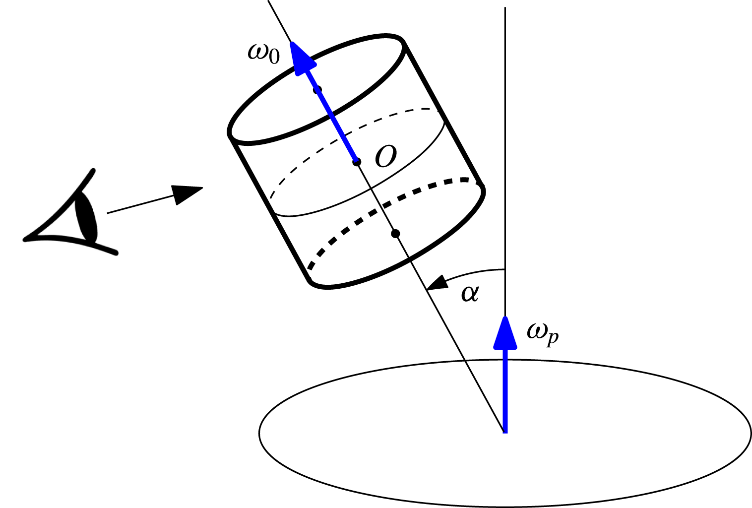
Schematic of the precessing cylinder.

A cylinder of height
 $H$
and radius
 $R$
is filled with an incompressible fluid of kinematic viscosity
 $\unicode[STIX]{x1D708}$
. All variables are non-dimensionalized using the cylinder radius
 $R$
as the length scale and the viscous time
 $R^{2}/\unicode[STIX]{x1D708}$
as the time scale. The cylinder is mounted at the centre of a horizontal table that rotates with angular velocity
 $\unicode[STIX]{x1D6FA}_{p}$
around the vertical axis, and the cylinder rotates with angular velocity
 $\unicode[STIX]{x1D6FA}_{0}$
about its axis, as shown in figure 1. The cylinder axis is tilted an angle
 $\unicode[STIX]{x1D6FC}$
relative to the vertical, and is at rest relative to the table.
There are four independent non-dimensional parameters governing the flow:
 $$\begin{eqnarray}\displaystyle & \text{Cylinder rotation}\quad \unicode[STIX]{x1D714}_{0}=\unicode[STIX]{x1D6FA}_{0}R^{2}/\unicode[STIX]{x1D708}, & \displaystyle\end{eqnarray}$$
 $$\begin{eqnarray}\displaystyle & \text{Precession rate}\quad \unicode[STIX]{x1D714}_{p}=\unicode[STIX]{x1D6FA}_{p}R^{2}/\unicode[STIX]{x1D708}, & \displaystyle\end{eqnarray}$$
 $$\begin{eqnarray}\displaystyle & \text{Aspect ratio}\quad \unicode[STIX]{x1D6E4}=H/R, & \displaystyle\end{eqnarray}$$
 $$\begin{eqnarray}\displaystyle & \text{Tilt angle}\quad \unicode[STIX]{x1D6FC}. & \displaystyle\end{eqnarray}$$
It is also convenient to introduce the Poincaré number
 $Po=\unicode[STIX]{x1D714}_{p}/\unicode[STIX]{x1D714}_{0}$
.
The governing equations are written using cylindrical coordinates
 $(r,\unicode[STIX]{x1D703},z)$
, where
 $z$
is in the direction of the cylinder axis, which is at rest relative to the rotating table, and the origin is at the cylinder centre
 $O$
, as shown in figure 1. The fluid domain is given by
 ${\mathcal{D}}=\{(r,\unicode[STIX]{x1D703},z)\in [0,1]\times [0,2\unicode[STIX]{x03C0}]\times [-\unicode[STIX]{x1D6E4}/2,\unicode[STIX]{x1D6E4}/2]\}$
. All terms that can be written as gradients are incorporated into the pressure gradient term. Since the solid-body rotation is a large component of the velocity, it is convenient to decompose the velocity as
 $\boldsymbol{v}=\boldsymbol{v}_{SB}+\boldsymbol{u}$
, where in cylindrical coordinates
 $\boldsymbol{v}_{SB}=(0,r\unicode[STIX]{x1D714}_{0},0)$
and the velocity deviation away from solid-body rotation is
 $\boldsymbol{u}=(u,v,w)$
. The governing equations for
 $\boldsymbol{u}$
, in the table frame of reference, are
 $$\begin{eqnarray}\unicode[STIX]{x2202}_{t}\boldsymbol{u}+(\boldsymbol{u}\boldsymbol{\cdot }\unicode[STIX]{x1D735})\boldsymbol{u}=-\unicode[STIX]{x1D735}p-2\unicode[STIX]{x1D74E}_{p}\times \boldsymbol{v}+\unicode[STIX]{x0394}\boldsymbol{u},\quad \unicode[STIX]{x1D735}\boldsymbol{\cdot }\boldsymbol{u}=0,\end{eqnarray}$$
with homogeneous boundary conditions
 $\boldsymbol{u}|_{\unicode[STIX]{x2202}{\mathcal{D}}}=0$
. The total angular velocity vector of the cylinder is
 $$\begin{eqnarray}\unicode[STIX]{x1D74E}_{total}=\unicode[STIX]{x1D74E}_{0}+\unicode[STIX]{x1D74E}_{p}=\unicode[STIX]{x1D714}_{p}\sin \unicode[STIX]{x1D6FC}\hat{\boldsymbol{y}}+(\unicode[STIX]{x1D714}_{0}+\unicode[STIX]{x1D714}_{p}\cos \unicode[STIX]{x1D6FC})\hat{\boldsymbol{z}}=\unicode[STIX]{x1D714}_{\bot }\hat{\boldsymbol{y}}+\unicode[STIX]{x1D714}_{a}\hat{\boldsymbol{z}},\end{eqnarray}$$
where
 $\unicode[STIX]{x1D714}_{a}$
is the rotation rate of the cylinder around its axis. The unit vector
 $\hat{\boldsymbol{y}}$
is orthogonal to the cylinder axis and is contained in the plane spanned by the angular velocities
 $\unicode[STIX]{x1D74E}_{0}$
and
 $\unicode[STIX]{x1D74E}_{p}$
. The component of
 $\unicode[STIX]{x1D74E}_{total}$
orthogonal to the cylinder axis,
 $\unicode[STIX]{x1D714}_{\bot }=\unicode[STIX]{x1D714}_{p}\sin \unicode[STIX]{x1D6FC}$
, is the forcing term in the cylinder frame that drives inertial waves. Since
 $\unicode[STIX]{x1D714}_{\bot }\,\hat{\boldsymbol{y}}$
is steady in the table frame, this forcing is periodic in the cylinder frame, with frequency
 $\unicode[STIX]{x1D714}_{0}$
. The cylinder frame is typically used in theoretical studies of inertial waves, whereas data acquisition and visualization in many precessing cylinder experiments are done in the table frame. The amplitude of the forcing is
 $\unicode[STIX]{x1D714}_{p}\sin \unicode[STIX]{x1D6FC}$
, which is proportional to
 $Po\sin \unicode[STIX]{x1D6FC}$
.
Some precessing cylinder studies call
 $\unicode[STIX]{x1D714}_{a}$
the Reynolds number
 $Re=\unicode[STIX]{x1D714}_{a}$
(e.g. Lagrange et al.
Reference Lagrange, Eloy, Nadal and Meunier2008, Reference Lagrange, Meunier, Nadal and Eloy2011; Meunier et al.
Reference Meunier, Eloy, Lagrange and Nadal2008). In rotation dominated flows, often instead of the Reynolds number, an Ekman number
 $Ek=\unicode[STIX]{x1D708}/(\unicode[STIX]{x1D6FA}_{0}(2R)^{2})=1/(4\unicode[STIX]{x1D714}_{0})$
is used (e.g. Manasseh Reference Manasseh1992, whose precessing cylinder experiments were conducted with
 $Ek\sim 10^{-5}$
). The largest
 $\unicode[STIX]{x1D714}_{0}=2\times 10^{4}$
we consider corresponds to
 $Ek=1.25\times 10^{-5}$
.
The inertial body force is the Coriolis term in (2.5). It can be split into two terms:
 $$\begin{eqnarray}\displaystyle & & \displaystyle -2\unicode[STIX]{x1D74E}_{p}\times \boldsymbol{v}=-2r\unicode[STIX]{x1D714}_{0}\unicode[STIX]{x1D714}_{p}\sin \unicode[STIX]{x1D6FC}\sin \unicode[STIX]{x1D703}\hat{\boldsymbol{z}}\nonumber\\ \displaystyle & & \displaystyle \quad +\,2\unicode[STIX]{x1D714}_{p}\sin \unicode[STIX]{x1D6FC}[(v\cot \unicode[STIX]{x1D6FC}-w\cos \unicode[STIX]{x1D703})\hat{\boldsymbol{r}}+(w\sin \unicode[STIX]{x1D703}-u\cot \unicode[STIX]{x1D6FC})\hat{\unicode[STIX]{x1D73D}}+(u\cos \unicode[STIX]{x1D703}-v\sin \unicode[STIX]{x1D703})\hat{\boldsymbol{z}}].\qquad \quad\end{eqnarray}$$
The body force depends explicitly on the azimuthal coordinate
 $\unicode[STIX]{x1D703}$
, it has azimuthal wavenumber
 $m=1$
due to the tilt angle
 $\unicode[STIX]{x1D6FC}$
, but is steady in the table frame.
The governing equations have been solved using a second-order time-splitting method, with space discretized via a Galerkin–Fourier expansion in
 $\unicode[STIX]{x1D703}$
and Chebyshev collocation in
 $r$
and
 $z$
. The spectral solver is based on that described by Mercader, Batiste & Alonso (Reference Mercader, Batiste and Alonso2010), with the inertial body force added. The numerical technique used is particularly well suited for the precessing flow where an
 $m=1$
azimuthal wavenumber is being driven that results in a non-zero velocity across the axis of the cylinder; the Chebyshev–Fourier decomposition used respects the parity conditions at the axis (Marques & Lopez Reference Marques and Lopez2001). It is the same code we have used in other studies of precessing cylinder flows (Marques & Lopez Reference Marques and Lopez2015; Lopez & Marques Reference Lopez and Marques2016b
). For the solutions presented in this study, we have used
 $n_{r}=n_{z}=64$
Chebyshev modes in the radial and axial directions and
 $n_{\unicode[STIX]{x1D703}}=130$
azimuthal Fourier modes.
The modal energies of the azimuthal Fourier components of a given solution are
 $$\begin{eqnarray}E_{m}=\frac{1}{2}\int _{z=-\unicode[STIX]{x1D6E4}/2}^{z=\unicode[STIX]{x1D6E4}/2}\int _{r=0}^{r=1}\boldsymbol{u}_{m}\boldsymbol{\cdot }\boldsymbol{u}_{m}^{\ast }r\,\text{d}r\,\text{d}z,\end{eqnarray}$$
where
 $\boldsymbol{u}_{m}$
is the
 $m$
th Fourier component of the velocity and
 $\boldsymbol{u}_{m}^{\ast }$
is its complex conjugate. These provide a convenient way to characterize the different states obtained. Also, it is convenient to consider the modal kinetic energies relative to the kinetic energy of solid-body rotation,
 $e_{m}=E_{m}/E_{SB}$
, where
 $E_{SB}=(1/8)\unicode[STIX]{x1D6E4}\unicode[STIX]{x1D714}_{0}^{2}$
. Other useful variables are the vorticity
 $\unicode[STIX]{x1D735}\times \boldsymbol{u}=(\unicode[STIX]{x1D709},\unicode[STIX]{x1D702},\unicode[STIX]{x1D701})$
, and the helicity
 ${\mathcal{H}}=\boldsymbol{u}\boldsymbol{\cdot }(\unicode[STIX]{x1D735}\times \boldsymbol{u})$
, both defined in terms of
 $\boldsymbol{u}$
, the deviation of the velocity away from solid-body rotation.
The system is equivariant to an inversion symmetry
 ${\mathcal{I}}$
, which is the combined action of rotation by angle
 $\unicode[STIX]{x03C0}$
about the cylinder axis and a reflection about the cylinder mid-height. The action of
 ${\mathcal{I}}$
on the position vector is
 ${\mathcal{I}}\boldsymbol{r}=-\boldsymbol{r}$
, and on the cylindrical coordinates the action is
 $(r,\unicode[STIX]{x1D703},z)\mapsto (r,\unicode[STIX]{x1D703}+\unicode[STIX]{x03C0},-z)$
. This motivates the definition of a global symmetry parameter,
 $S=\Vert \boldsymbol{u}-{\mathcal{I}}\boldsymbol{u}\Vert _{2}$
(Marques & Lopez Reference Marques and Lopez2015). The action of
 ${\mathcal{I}}$
on the velocity, vorticity, and the helicity is
 $$\begin{eqnarray}{\mathcal{A}}({\mathcal{I}})(u,v,w,\unicode[STIX]{x1D709},\unicode[STIX]{x1D702},\unicode[STIX]{x1D701},{\mathcal{H}})(r,\unicode[STIX]{x1D703},z,t)=(u,v,-w,-\unicode[STIX]{x1D709},-\unicode[STIX]{x1D702},\unicode[STIX]{x1D701},-{\mathcal{H}})(r,\unicode[STIX]{x1D703}+\unicode[STIX]{x03C0},-z,t).\end{eqnarray}$$
The base state (BS) (also referred to as the forced response), is the unique solution of the governing equations for small enough rotation rates; it is steady and
 ${\mathcal{I}}$
-symmetric:
 ${\mathcal{I}}(\text{BS})=\text{BS}$
. The square of
 ${\mathcal{I}}$
is the identity, and so this symmetry generates the symmetry group
 $Z_{2}$
, consisting of two elements, the identity and
 ${\mathcal{I}}$
. Dynamical systems theory says that for a Hopf bifurcation from an
 ${\mathcal{I}}$
-symmetric steady solution, such as BS, resulting in a limit cycle (LC) with period
 $\unicode[STIX]{x1D70F}$
, there are only two possible scenarios (see Kuznetsov Reference Kuznetsov2004, chap. 7, Theorem 7.8):
 $$\begin{eqnarray}{\mathcal{I}}(\text{LC}(t))=\left\{\begin{array}{@{}ll@{}}{\mathcal{I}}(\text{LC}(t))=\text{LC}(t),\quad & \text{LC is an }F\text{-cycle},\\ {\mathcal{I}}(\text{LC}(t))=\text{LC}(t+\unicode[STIX]{x1D70F}/2),\quad & \text{LC is an }S\text{-cycle}.\end{array}\right.\end{eqnarray}$$
Either the bifurcated periodic solution LC is
 $Z_{2}$
-equivariant (an
 $F$
-cycle, which we shall call LCs), or the
 $Z_{2}$
symmetry is broken at the bifurcation and the periodic solution (an
 $S$
-cycle, which we shall call LCa) is not
 $Z_{2}$
symmetric, but instead has a spatio-temporal symmetry. This spatio-temporal symmetry is such that applying the
 $Z_{2}$
symmetry is the same as advancing the solution for half a period in time. Therefore an
 $S$
-cycle LCa has a spatio-temporal symmetry
 $$\begin{eqnarray}{\mathcal{I}}^{st}(\text{LCa}(t))={\mathcal{I}}(\text{LCa}(t+\unicode[STIX]{x1D70F}/2))=\text{LCa}(t),\end{eqnarray}$$
and LCa as a set, is
 ${\mathcal{I}}$
-symmetric: applying
 ${\mathcal{I}}$
to a point of LCa (i.e. to LCa
 $(t)$
at a particular time
 $t=t^{\star }$
) results in another point of LCa (i.e. LCa(
 $t\neq t^{\star }$
), such that
 ${\mathcal{I}}(\text{LC})=\text{LC}$
. The concept of setwise
 ${\mathcal{I}}$
invariance can also be applied to more complex solutions, like two- or three-torus states, or strange attractors, although for these states the setwise invariance does not necessarily correspond to the half-period-flip
 ${\mathcal{I}}^{st}$
symmetry (2.11). Some examples in other fluid flows can be found in Lopez & Marques (Reference Lopez and Marques2004), Abshagen et al. (Reference Abshagen, Lopez, Marques and Pfister2005a
,Reference Abshagen, Lopez, Marques and Pfister
b
), Lopez & Marques (Reference Lopez and Marques2005), Lopez (Reference Lopez2006), Marques & Lopez (Reference Marques and Lopez2006), Abshagen et al. (Reference Abshagen, Lopez, Marques and Pfister2008) and Altmeyer et al. (Reference Altmeyer, Do, Marques and Lopez2012).
3 Background
Rapidly rotating flows can sustain inertial waves, and these have been observed in a large variety of flows. Inertial waves are rapidly damped by viscous effects, and in order to observe them they need to be continuously excited by some driving force. When the driving acts over the whole domain, such as by the Coriolis force in precessing flows, the inertial waves tend to resemble some of the inviscid Kelvin eigenmodes of the domain. In contrast, when the driving force is localized, beams of inertial waves are observed to emerge from the localized forced region (McEwan Reference McEwan1970). In the precessing cylinder flow, the boundary layers near the corners where the cylinder endwalls meet the sidewall provide the localized driving resulting in the wave beams (Wood Reference Wood1965). The angle
 $\unicode[STIX]{x1D6FD}$
between the beams and the plane orthogonal to the cylinder axis is determined from the dispersion relation of the linear inviscid problem (Greenspan Reference Greenspan1968):
 $$\begin{eqnarray}2\cos \unicode[STIX]{x1D6FD}=\unicode[STIX]{x1D714}_{0}/\unicode[STIX]{x1D714}_{a}=\unicode[STIX]{x1D714}_{0}/(\unicode[STIX]{x1D714}_{0}+\unicode[STIX]{x1D714}_{p}\cos \unicode[STIX]{x1D6FC})=1/(1+Po\cos \unicode[STIX]{x1D6FC}),\end{eqnarray}$$
which is the ratio between the forcing frequency and the axial component of the angular velocity of the cylinder. In other studies (e.g. Lagrange et al.
Reference Lagrange, Eloy, Nadal and Meunier2008, Reference Lagrange, Meunier, Nadal and Eloy2011; Meunier et al.
Reference Meunier, Eloy, Lagrange and Nadal2008),
 $2\cos \unicode[STIX]{x1D6FD}$
is called
 $\unicode[STIX]{x1D714}$
, and they also use a Rossby number
 $Ro=Po\sin \unicode[STIX]{x1D6FC}/(1+Po\cos \unicode[STIX]{x1D6FC})$
, which is proportional to the amplitude of the forcing.
The Kelvin eigenmodes are the solution of the (inviscid) Euler equations linearized about the solid-body rotation state. The singular perturbation of vanishing viscosity means that the Kelvin modes do not satisfy the no-slip boundary conditions for the velocity. They only satisfy the no-penetration condition, i.e. that the normal velocity component is zero at the boundary of the domain. The Kelvin modes are characterized by three integers
 $(k,m,n)$
, related to the number of zeros of the eigenmode in the radial, azimuthal and axial directions, respectively. For example, the vertical velocity of the
 $(k,m,n)$
Kelvin mode (
 $K_{kmn}$
for short) in the cylinder reference frame is explicitly given by
 $$\begin{eqnarray}w_{kmn}(r,\unicode[STIX]{x1D703},z,t)=c\text{J}_{m}(a_{k}r)\sin n\unicode[STIX]{x03C0}z^{\ast }\sin (m\unicode[STIX]{x1D703}+\unicode[STIX]{x1D70E}t),\end{eqnarray}$$
where
 $\text{J}_{m}$
is an integer Bessel function,
 $c$
is a normalization constant,
 $\unicode[STIX]{x1D70E}>0$
is the temporal frequency in the cylinder frame (we take
 $\unicode[STIX]{x1D70E}$
positive, which fixes the sign of
 $c$
),
 $z^{\ast }=z/\unicode[STIX]{x1D6E4}+1/2\in [0,1]$
and
 $a_{k}$
is the
 $k$
-zero of a complicated Bessel equation that also depends on
 $n$
,
 $m$
and
 $\unicode[STIX]{x1D6E4}$
(Lord Kelvin 1880; Greenspan Reference Greenspan1968):
 $$\begin{eqnarray}a_{k}J_{m}^{\prime }(a_{k})+m\sqrt{1+\left(\frac{\unicode[STIX]{x1D6E4}a_{k}}{n\unicode[STIX]{x03C0}}\right)^{2}}\text{J}_{m}(a_{k})=0.\end{eqnarray}$$
The number of zeros in the bulk (excluding the boundaries and the cylinder axis) in the azimuthal and axial directions is given by
 $(2|m|,n-1)$
, except in the axisymmetric case
 $m=0$
where there is no dependence on
 $\unicode[STIX]{x1D703}$
. The number of zeros in the radial direction is
 $k-1$
for
 $m>0$
and
 $k$
for
 $m<0$
. The integers
 $k$
and
 $n$
are always positive, while the sign of
 $m$
is associated with the azimuthal drift frequency of the Kelvin mode in the cylinder reference frame; the Kelvin modes are rotating waves.
The relationship between the cylinder and table frames is easy to obtain. The cylindrical coordinates of a fluid parcel
 $P$
in the two reference frames are
 $\boldsymbol{r}=(r,\unicode[STIX]{x1D703}_{C},z)=(r,\unicode[STIX]{x1D703}_{T},z)$
, where the sub-indexes
 $_{C}$
and
 $_{T}$
refer to the cylinder and table frames, and
 $\unicode[STIX]{x1D703}_{T}=\unicode[STIX]{x1D703}_{C}+\unicode[STIX]{x1D714}_{0}t$
. The two reference frames have the same origin, therefore the difference in their velocities is due to the angular velocity
 $\unicode[STIX]{x1D74E}_{0}=\unicode[STIX]{x1D714}_{0}\hat{\boldsymbol{z}}$
:
 $$\begin{eqnarray}\boldsymbol{v}_{T}=\boldsymbol{v}_{C}+\unicode[STIX]{x1D74E}_{0}\times \boldsymbol{r}=\boldsymbol{v}_{C}+(0,\unicode[STIX]{x1D714}_{0}r,0).\end{eqnarray}$$
Since in the table frame we use the deviation of
 $\boldsymbol{v}_{T}$
with respect to the solid-body rotation of the cylinder,
 $\boldsymbol{u}=\boldsymbol{v}_{T}-\unicode[STIX]{x1D74E}_{0}\times \boldsymbol{r}=\boldsymbol{v}_{C}$
, the velocities
 $\boldsymbol{u}$
and
 $\boldsymbol{v}_{C}$
are the same, except that they refer to the different coordinates. For example,
 $K_{kmn}$
in the table frame is obtained by replacing
 $\unicode[STIX]{x1D703}_{C}$
by
 $\unicode[STIX]{x1D703}_{T}-\unicode[STIX]{x1D714}_{0}t$
in (3.2):
 $$\begin{eqnarray}w_{kmn}^{T}(r,\unicode[STIX]{x1D703},z,t)=c\text{J}_{m}(a_{k}r)\sin n\unicode[STIX]{x03C0}z^{\ast }\sin (m\unicode[STIX]{x1D703}+\unicode[STIX]{x1D714}t),\quad \unicode[STIX]{x1D714}=\unicode[STIX]{x1D70E}-m\unicode[STIX]{x1D714}_{0}.\end{eqnarray}$$
From the phase of the last factor in (3.2) and (3.5), we obtain the azimuthal drift frequency of the rotating wave pattern in each of the two frames:
 $$\begin{eqnarray}\unicode[STIX]{x1D70E}^{\mathit{drift}}=\frac{\text{d}\unicode[STIX]{x1D703}_{C}}{\text{d}t}=-\frac{\unicode[STIX]{x1D70E}}{m},\quad \unicode[STIX]{x1D714}^{\mathit{drift}}=\frac{\text{d}\unicode[STIX]{x1D703}_{T}}{\text{d}t}=-\frac{\unicode[STIX]{x1D714}}{m},\quad \unicode[STIX]{x1D70E}^{\mathit{drift}}=\unicode[STIX]{x1D714}^{\mathit{drift}}-\unicode[STIX]{x1D714}_{0},\end{eqnarray}$$
where we have used
 $\unicode[STIX]{x1D714}$
for frequencies in the table reference frame and
 $\unicode[STIX]{x1D70E}$
for frequencies in the cylinder reference frame. Positive (negative) azimuthal drift frequencies correspond to prograde (retrograde) rotating waves. In the cylinder frame, prograde (retrograde) rotating waves have
 $m<0$
(
 $m>0$
) because
 $\unicode[STIX]{x1D70E}>0$
. In the table frame, the prograde or retrograde character of the rotating wave depends on the signs of
 $\unicode[STIX]{x1D714}$
and
 $m$
. These rotating waves are time periodic, with period
 $\unicode[STIX]{x1D70F}^{C}=2\unicode[STIX]{x03C0}/\unicode[STIX]{x1D70E}$
in the cylinder frame, and
 $\unicode[STIX]{x1D70F}^{T}=2\unicode[STIX]{x03C0}/|\unicode[STIX]{x1D714}|$
in the table frame.
It is also interesting to compute the action of the inversion symmetry on the Kelvin eigenmodes
 $K_{kmn}$
:
 $$\begin{eqnarray}{\mathcal{A}}({\mathcal{I}})(u,v,w)_{kmn}(r,\unicode[STIX]{x1D703},z,t)=(-1)^{m+n}(u,v,w)_{kmn}(r,\unicode[STIX]{x1D703},z,t).\end{eqnarray}$$
Kelvin eigenmodes with
 $m+n$
even are
 ${\mathcal{I}}$
-symmetric, while those with
 $m+n$
odd are not. When exploring the possibility of spatio-temporal symmetries, it is important to consider the effect of advancing a Kelvin eigenmode by half a period in time:
 $$\begin{eqnarray}(u,v,w)_{kmn}(r,\unicode[STIX]{x1D703},z,t+\unicode[STIX]{x1D70F}/2)=-(u,v,w)_{kmn}(r,\unicode[STIX]{x1D703},z,t).\end{eqnarray}$$
The combined action of the inversion symmetry and advancing half a period is
 $$\begin{eqnarray}{\mathcal{A}}({\mathcal{I}})(u,v,w)_{kmn}(r,\unicode[STIX]{x1D703},z,t+\unicode[STIX]{x1D70F}/2)=(-1)^{m+n+1}(u,v,w)_{kmn}(r,\unicode[STIX]{x1D703},z,t).\end{eqnarray}$$
Therefore, when
 $m+n$
is odd, the Kelvin eigenmode has a spatio-temporal symmetry: applying inversion symmetry and advancing half a period. This type of spatio-temporal symmetry, whose square is the identity, generates a spatio-temporal
 $Z_{2}$
symmetry group. This type of spatio-temporal symmetry is common in many hydrodynamic flows, and is often called a half-period-flip symmetry (Marques & Lopez Reference Marques and Lopez1997; Marques, Lopez & Blackburn Reference Marques, Lopez and Blackburn2004; Blackburn, Marques & Lopez Reference Blackburn, Marques and Lopez2005; Leung et al.
Reference Leung, Hirsa, Blackburn, Marques and Lopez2005).
In the precessing flows considered here, the spatial structure of the base state BS, corresponding to the overturning flow induced by the tilt of the cylinder, tends to resemble
 $K_{111}$
, and both are
 ${\mathcal{I}}$
-symmetric. Each Kelvin mode has a well-defined frequency
 $\unicode[STIX]{x1D70E}_{kmn}^{K}$
that depends on the geometry
 $\unicode[STIX]{x1D6E4}$
, the axial angular velocity of the cylinder
 $\unicode[STIX]{x1D714}_{a}$
, and the integers
 $(k,m,n)$
. In the cylinder frame, BS is time periodic with a frequency equal to the forcing frequency, and in general this does not coincide with the frequency of
 $K_{111}$
. Therefore, what is observed is the forced solution BS, not the natural Kelvin mode of the system. The situation is very similar to what happens with a damped harmonically forced oscillator; the response is a combination of a damped natural oscillation (analogous to the Kelvin modes) with the frequency of the oscillator that is detuned by the damping, and a sustained oscillation with the forcing frequency (the forced response BS). The natural oscillation decays due to viscous damping, and only the forced oscillation remains. Kelvin modes can only be observed if the forcing frequency is tuned to the frequency of the Kelvin mode, i.e. if the system is subjected to resonant forcing. The condition for resonant forcing with
 $K_{kmn}$
is
 $\unicode[STIX]{x1D714}_{0}=\unicode[STIX]{x1D70E}_{kmn}^{K}$
. As the frequencies of the Kelvin modes are dense in the interval
 $(0,2\unicode[STIX]{x1D714}_{a})$
, there are Kelvin eigenmodes with frequencies arbitrarily close to a given forcing frequency
 $\unicode[STIX]{x1D714}_{0}$
in this interval. We can define a detuning parameter
 $$\begin{eqnarray}\unicode[STIX]{x1D6FF}_{1}=\left|\frac{\unicode[STIX]{x1D70E}_{kmn}^{K}}{\unicode[STIX]{x1D714}_{0}}-1\right|,\end{eqnarray}$$
measuring the proximity of a given Kelvin mode to resonance with forcing frequency
 $\unicode[STIX]{x1D714}_{0}$
. In general, the modes that are close to resonance tend to have large values of
 $k$
,
 $|m|$
and
 $n$
(except in specifically tuned cases), and are rapidly damped by viscosity, therefore they cannot be observed in real situations. Only the forced mode remains.
Several recent studies have focused on the analysis of triadic resonances (Lagrange et al.
Reference Lagrange, Meunier, Nadal and Eloy2011; Albrecht et al.
Reference Albrecht, Blackburn, Lopez, Manasseh and Meunier2015; Marques & Lopez Reference Marques and Lopez2015; Lopez & Marques Reference Lopez and Marques2016b
), where the forcing frequency was tuned to the frequency of the overturning Kelvin mode, i.e.
 $\unicode[STIX]{x1D714}_{0}=\unicode[STIX]{x1D70E}_{111}^{K}$
. Moreover, parameters of the system were tuned so that this mode is also in triadic resonance with two additional Kelvin modes,
 $K_{k_{1}m_{1}n_{1}}$
and
 $K_{k_{2}m_{2}n_{2}}$
, satisfying the resonance conditions
 $$\begin{eqnarray}|n_{1}-n_{2}|=1,\quad s_{1}m_{1}+s_{2}m_{2}=1,\quad \text{and}\quad s_{1}\frac{\unicode[STIX]{x1D70E}_{k_{1}m_{1}n_{1}}}{\unicode[STIX]{x1D714}_{0}}+s_{2}\frac{\unicode[STIX]{x1D70E}_{k_{2}m_{2}n_{2}}}{\unicode[STIX]{x1D714}_{0}}=\frac{\unicode[STIX]{x1D70E}_{111}}{\unicode[STIX]{x1D714}_{0}}=1,\end{eqnarray}$$
where
 $|s_{1}|=|s_{2}|=1$
. This is called the 1 :
 $m_{1}$
:
 $m_{2}$
resonance. In all cases we know of in the literature,
 $s_{1}=s_{2}=1$
and one of the
 $m$
is positive and the other negative, i.e. one of the modes is prograde and the other is retrograde in the cylinder frame. As there are two triadic resonance conditions to be satisfied, two of the system parameters must be carefully tuned in order to observe the triadic resonance, typically the aspect ratio and the Poincaré number. Therefore, there are only a few small regions of parameter space corresponding to tuned triadic resonances between Kelvin modes. In the present study, we explore the dynamics of the precessing cylinder flow away from such triadic resonances, which is the generic situation. One of the goals is to understand what aspects of the dynamics observed in the previous studies are specific to the Kelvin triadic resonances, and which are generic in precessing flows.
In rotating cylinder flows, the boundary layers provide the localized driving that generates inertial wave beams, particularly near the corners where the cylinder endwalls meet the sidewall (Lopez & Marques Reference Lopez and Marques2011, Reference Lopez and Marques2014; Lopez & Gutierrez-Castillo Reference Lopez and Gutierrez-Castillo2016; Lopez & Marques Reference Lopez and Marques2016a ). In precessing flows, these wave beams are not axisymmetric due to the presence of the overturning flow, which completely breaks the rotational symmetry. It has been observed in many rotating flows that when the wave beams retrace themselves, they are reinforced, and intense wave beams are formed that can influence the dynamics. This situation has not been studied in detail in precessing cylinder flows.
Here, we study two regimes away from Kelvin mode triadic resonance: one where according to the angle of propagation determined from the linear inviscid dispersion relation (3.1) the wave beams would retrace themselves, and another where they do not. In the literature, the retracing and non-retracing cases are sometimes referred to as periodic and quasi-periodic orbits of the characteristics (e.g. Rieutord, Georgeot & Valdettaro Reference Rieutord, Georgeot and Valdettaro2001). The two cases we consider have the same geometry: aspect ratio
 $\unicode[STIX]{x1D6E4}=1.33$
and tilt angle
 $\unicode[STIX]{x1D6FC}=3^{\circ }$
. Whether characteristics retrace themselves or not is then solely determined by the Poincaré number
 $Po$
. Retracing characteristics that go through the centre of the cylinder require
 $\tan \unicode[STIX]{x1D6FD}=\unicode[STIX]{x1D6E4}/2$
, i.e.
 $\unicode[STIX]{x1D6FD}=\pm 33.6^{\circ }$
, for which
 $Po=-0.4$
. The non-retracing case we consider is
 $Po=-0.3745$
with
 $\unicode[STIX]{x1D6FD}=\pm 37.0^{\circ }$
. The corresponding characteristics emerging from the corners where the endwalls meet the sidewall are shown in figure 2(c,f). The 6.3 % difference in
 $Po$
changes the nature of the characteristics. The frequencies of
 $K_{111}$
in the two cases are given by
 $\unicode[STIX]{x1D70E}_{111}^{K}/\unicode[STIX]{x1D714}_{0}=0.8106$
for
 $Po=-0.4$
and
 $\unicode[STIX]{x1D70E}_{111}^{K}/\unicode[STIX]{x1D714}_{0}=0.8449$
for
 $Po=-0.3745$
. Both cases are far from the resonance condition
 $\unicode[STIX]{x1D70E}_{111}^{K}/\unicode[STIX]{x1D714}_{0}=1$
.
There is also the possibility that two Kelvin modes are close to triadic resonance with the forced
 $(1,1,1)$
flow BS. These triadic resonances between a forced flow and natural Kelvin modes have been studied in a model precessing cylinder flow problem (Lagrange et al.
Reference Lagrange, Meunier and Eloy2016), and will also be explored in the present paper. In order to measure how close to resonance two natural Kelvin modes,
 $K_{k_{1}m_{1}n_{1}}$
and
 $K_{k_{2}m_{2}n_{2}}$
, are with the forced
 $(1,1,1)$
BS, we introduce the detuning parameter
 $$\begin{eqnarray}\unicode[STIX]{x1D6FF}_{3}=\left|s_{1}\frac{\unicode[STIX]{x1D70E}_{k_{1}m_{1}n_{1}}}{\unicode[STIX]{x1D714}_{0}}+s_{2}\frac{\unicode[STIX]{x1D70E}_{k_{2}m_{2}n_{2}}}{\unicode[STIX]{x1D714}_{0}}-1\right|,\end{eqnarray}$$
where
 $|n_{1}-n_{2}|=1$
,
 $s_{1}m_{1}+s_{2}m_{2}=1$
and
 $|s_{1}|=|s_{2}|=1$
, as in (3.11).
4 Base states
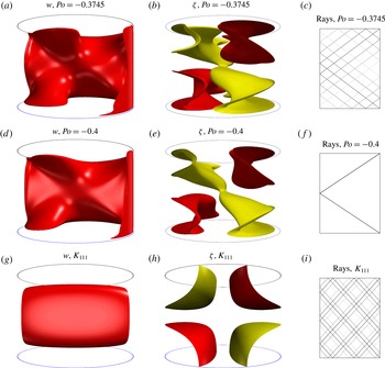
For the basic state (BS) at
 $\unicode[STIX]{x1D714}_{0}=4000$
,
 $\unicode[STIX]{x1D6E4}=1.33$
and
 $\unicode[STIX]{x1D6FC}=3^{\circ }$
, isosurfaces of axial velocity at
 $w=2$
are shown in (a) for
 $Po=-0.3745$
and (d) for
 $Po=-0.4$
. The corresponding axial vorticity isosurfaces at
 $\unicode[STIX]{x1D701}=-400$
and 300 are shown in (b) for
 $Po=-0.3745$
and (e) for
 $Po=-0.4$
; the
 $\unicode[STIX]{x1D701}$
isosurfaces are clipped at
 $r=0.915$
. The view has the two rotation vectors in the page. For the Kelvin mode
 $K_{111}$
at
 $\unicode[STIX]{x1D6E4}=1.33$
,
 $\unicode[STIX]{x1D6FC}=3^{\circ }$
, (g,h) show its isosurfaces of
 $w$
and
 $\unicode[STIX]{x1D701}$
. The corresponding characteristics of the linear inviscid system in a meridional plane
 $(r,z)\in [0,1]\times [-0.5\unicode[STIX]{x1D6E4},0.5\unicode[STIX]{x1D6E4}]$
, emerging from the corners, are shown in the third column (c,f,i).

The base states corresponding to the two cases considered are shown in figure 2. Figure 2(a,d) shows an isosurface of the vertical velocity at a positive level close to zero (
 $w=2$
), showing the upward moving part of the overturning flow. The isosurfaces are not planar but have substantial deformations due to the presence of inertial wave beams. As the inertial waves are shear waves, isosurfaces of the vertical vorticity
 $\unicode[STIX]{x1D701}$
based on the velocity deviation away from solid-body rotation (
 $\unicode[STIX]{x1D701}$
is very small for a pure overturning flow) are shown in figure 2(b,e) in order to distinguish the beams from the overturning flow. The wave beams are clearly seen in these figures. They emerge from the cylinder boundary layers, near the corners where the cylinder endwalls meet the sidewall, but they are not conical waves. This is because the overturning flow, and the Coriolis force that generates it, are not axisymmetric. The vorticity isosurfaces have been clipped at
 $r=0.915$
. This has been done because inside the boundary layers the vorticity changes substantially, and any isosurface of
 $\unicode[STIX]{x1D701}$
has a cylindrical sheet near the sidewall that hinders visualization of
 $\unicode[STIX]{x1D701}$
in the bulk. Figure 2(c,f) shows rays (characteristics of the linear inviscid equations) emerging from the corners at the angle
 $\unicode[STIX]{x1D6FD}$
corresponding to the given value of the Poincaré number
 $Po$
. For the non-retracing case
 $Po=-0.3745$
with
 $\unicode[STIX]{x1D6FD}=\pm 37.0^{\circ }$
, shown in figure 2(a–c), the vorticity isosurface in figure 2(b) fills a substantial part of the bulk, while in the retracing case, with
 $Po=-0.4$
and
 $\unicode[STIX]{x1D6FD}=\pm 33.6^{\circ }$
, figure 2(e) shows that the wave beams are narrower and occupy a smaller fraction of the bulk. It is worth noting that the width of the wave beams is large due to viscous effects for the
 $\unicode[STIX]{x1D714}_{0}$
considered;
 $\unicode[STIX]{x1D714}_{0}$
would need to be increased by several orders of magnitude in order to have very narrow beams that resemble the linear characteristics of the inviscid problem depicted in figure 2(c,f) (Lopez & Marques Reference Lopez and Marques2014). In figure 2(g,h,i), contours of axial velocity and axial vorticity, and characteristics emerging from the corners, are shown for the
 $K_{111}$
mode of the cylinder, corresponding to the inviscid linear theory with the same geometry
 $\unicode[STIX]{x1D6E4}=1.33$
. The isosurfaces are very smooth, and do not have boundary layers or beams. These two cases (
 $Po=-0.3745$
and
 $-0.4$
) are far from resonance with
 $K_{111}$
and the characteristics for all three cases are very different. For
 $K_{111}$
, the angle
 $\unicode[STIX]{x1D6FD}=\pm 47.6^{\circ }$
. This example clearly shows that the rays corresponding to Kelvin modes are generally not retracing, as was also discussed in detail in Lopez & Marques (Reference Lopez and Marques2014).
5 Instabilities of the base state
Variation of
 $e_{0}$
with
 $\unicode[STIX]{x1D714}_{0}$
for (a)
 $Po=-0.3745$
and (b)
 $Po=-0.4$
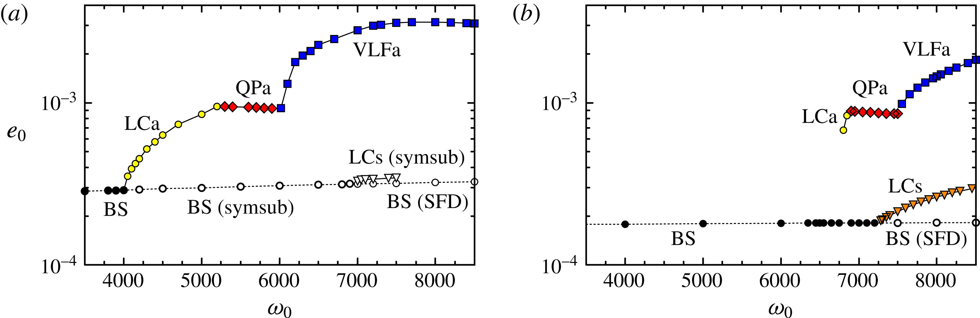
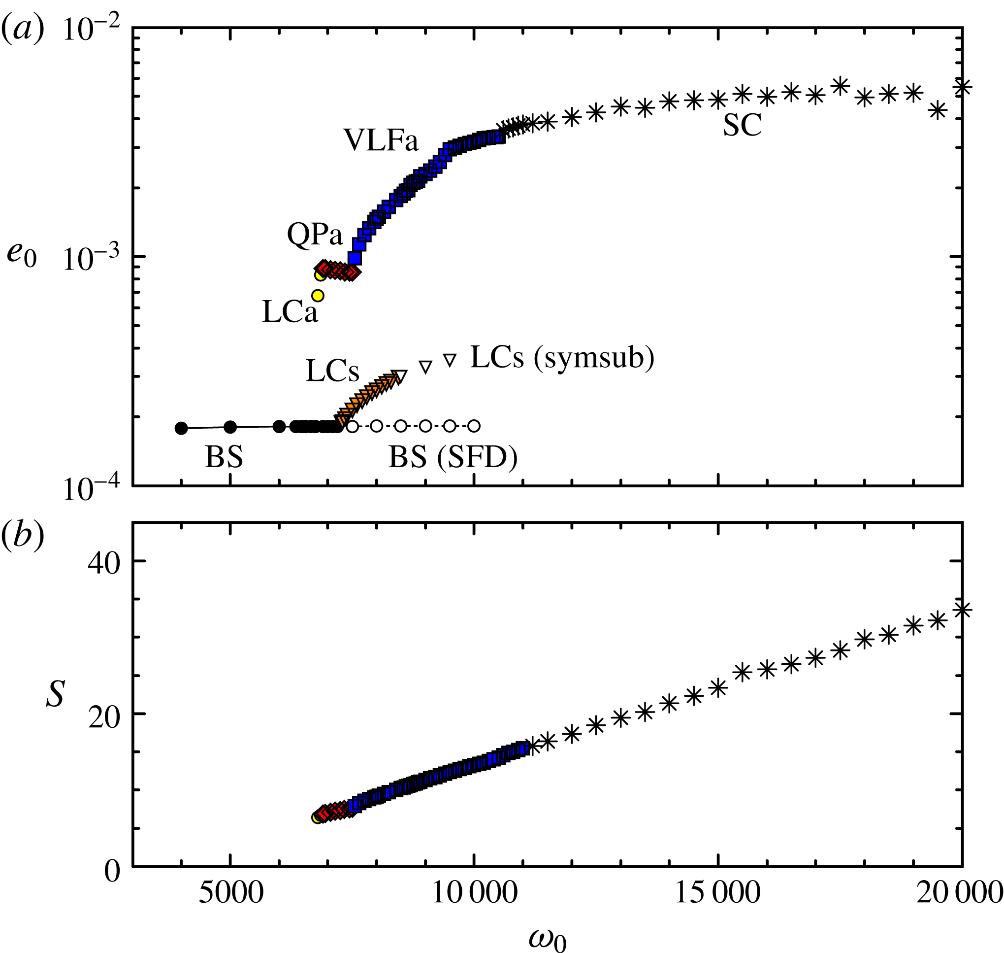
, for the states as indicated (see table 1 for details of these states). The states with filled symbols are stable and those with open symbols are unstable. The unstable states BS (symsub) and LCs (symsub) were computed in the
 ${\mathcal{I}}$
-symmetric subspace, and BS (SFD) was computed using the selective-frequency-damping (SFD) method.

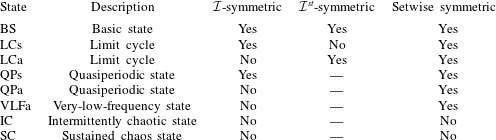
List of solution states, their acronyms and their invariances (see the discussion on symmetries at the end of § 2 for details).

We now explore how the flow responds as the effects of viscosity are reduced by increasing
 $\unicode[STIX]{x1D714}_{0}$
and
 $\unicode[STIX]{x1D714}_{p}$
whilst keeping their ratio,
 $Po$
, and the geometry
 $\unicode[STIX]{x1D6E4}=1.33$
and
 $\unicode[STIX]{x1D6FC}=3^{\circ }$
, fixed. Figure 3 summarizes the states that are found as
 $\unicode[STIX]{x1D714}_{0}$
is increased for the two cases,
 $Po=-0.3745$
(non-retracing rays) and
 $Po=-0.4$
(retracing rays), in terms of
 $e_{0}$
, the azimuthal average of the kinetic energy in the deviation away from solid-body rotation relative to the kinetic energy of the solid-body rotation corresponding to
 $\unicode[STIX]{x1D714}_{0}$
. This was found to be a convenient global measure for all the various states found, which have many differences in their spatio-temporal characteristics; table 1 lists these states and their invariances. In the following subsections, the details of the spatio-temporal characteristics of the various states will be described, as well as how the unstable states (shown with open symbols) have been computed. In spite of the fact that the two cases differ by only approximately 6 % in Poincaré number, there are significant differences in the sequences of instabilities and bifurcations. These are analysed in detail, and compared with the inviscid theory, in terms of Kelvin modes and resonances, in the following subsections.
5.1 The
 $Po=-0.3745$
case (non-retracing rays)

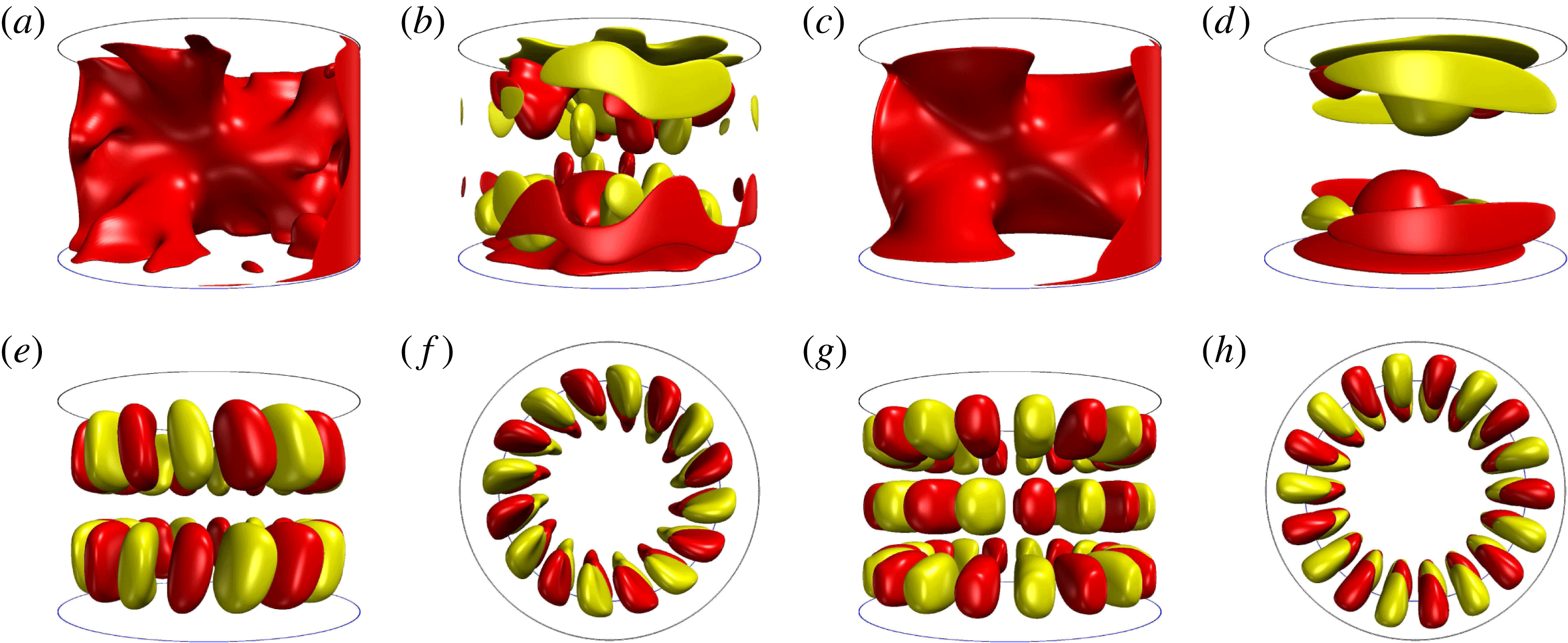
For LCa at
 $\unicode[STIX]{x1D714}_{0}=4500$
and
 $Po=-0.3745$
, shown are isosurfaces of (a)
 $w=2$
and (b)
 ${\mathcal{H}}=\pm 3\times 10^{5}$
, and of the (unstable) BS at the same parameters (computed in the
 ${\mathcal{I}}$
-symmetric subspace) with (c)
 $w=2$
and (d)
 ${\mathcal{H}}=\pm 3\times 10^{5}$
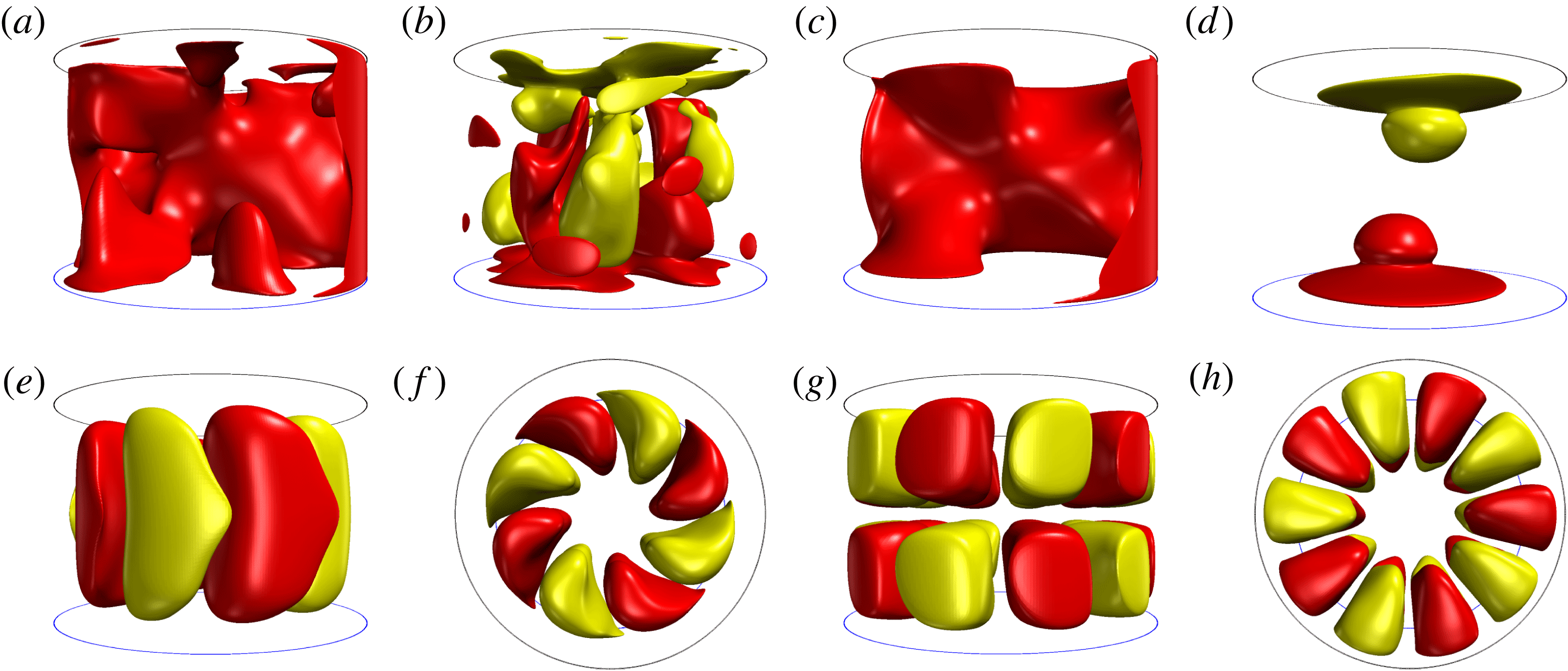
. The online supplementary movie available at https://doi.org/10.1017/jfm.2017.922 shows an animation of
 ${\mathcal{H}}$
for LCa over one period
 $\unicode[STIX]{x1D70F}_{\mathit{LCa}}=3.24\times 10^{-4}$
. Isosurfaces of the (e,f)
 $m=4$
and (g,h)
 $m=5$
azimuthal Fourier components of
 $w$
at levels
 $w=\pm 30$
are shown in two orthogonal views.

In this section, we consider the generic situation, away from triadic resonances of Kelvin modes and away from retracing inertial wave beams. Increasing
 $\unicode[STIX]{x1D714}_{0}$
with
 $Po=-0.3745$
fixed, the base state becomes unstable at
 $\unicode[STIX]{x1D714}_{0}\approx 3992$
in a Hopf bifurcation, resulting in a time periodic limit cycle solution LCa. The structure of LCa is shown in figure 4 for
 $\unicode[STIX]{x1D714}_{0}=4500$
. The isosurface of
 $w$
in figure 4(a) resembles that of the basic state, but additional structures are present in the interior emerging from the endwalls. The helicity contours in figure 4(b) show the presence of columnar helical structures in the bulk. These columns are absent in BS (figure 4
d). The unstable BS has been computed by restricting the simulations to the
 ${\mathcal{I}}$
-invariant subspace, and the
 $w$
isosurfaces of BS are shown in figure 4(c). The presence of the helical columns in LCa greatly distorts the inertial wave beams. The columnar structures, and their temporal evolution, can be appreciated in the supplementary online movie. The helical columns resemble a rotating wave, but there are significant distortions during the period of the solution.
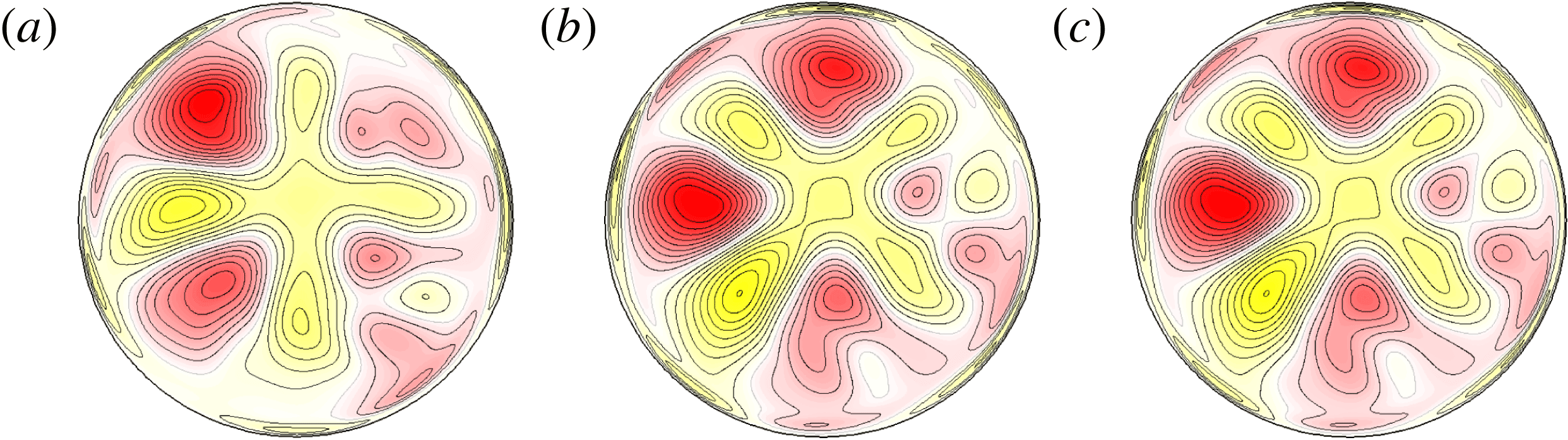
Contours of (a)
 ${\mathcal{H}}(t_{0})$
, (b)
 ${\mathcal{I}}({\mathcal{H}}(t_{0}))$
and (c)
 ${\mathcal{H}}(t_{0}+\unicode[STIX]{x1D70F}/2)$
at
 $z=\unicode[STIX]{x1D6E4}/4$
for LCa at
 $\unicode[STIX]{x1D714}_{0}=4500$
and
 $Po=-0.3745$
. Contour levels are
 ${\mathcal{H}}\in [-7.6\times 10^{5},7.6\times 10^{5}]$
.

Figure 5(a) shows contours of helicity in the plane
 $z=\unicode[STIX]{x1D6E4}/4$
for LCa at
 $\unicode[STIX]{x1D714}_{0}=4500$
. The helicity columns rotate, while the overturning flow remains fixed in the table frame, and the interaction between the columns and the overturning flow results in the observed distortions with time. The frequency of the bifurcated solution LCa is
 $\unicode[STIX]{x1D714}_{\mathit{LCa}}\approx 1.94\times 10^{4}$
, between four and five times
 $\unicode[STIX]{x1D714}_{0}=4500$
.
The base state is equivariant with respect to the inversion symmetry
 ${\mathcal{I}}$
. The ‘a’ in LCa signifies that it is not
 ${\mathcal{I}}$
-equivariant. This can be readily observed in figure 5(a,b) showing the helicity contours of LCa and of the transformed field by
 ${\mathcal{I}}$
. According to (2.9), the helicity should simply change sign if the solution were symmetric (i.e.
 ${\mathcal{I}}$
-equivariant). This is not the case, LCa is not
 ${\mathcal{I}}$
-symmetric. The non-symmetry of LCa can be quantified by the symmetry parameter, which for the case shown in figure 5 is
 $S=4.12$
. As described at the end of § 2, the limit cycle bifurcating from an
 ${\mathcal{I}}$
-equivariant steady state (BS) is either
 ${\mathcal{I}}$
-equivariant (an
 $F$
-cycle), or the
 ${\mathcal{I}}$
-symmetry is broken at the bifurcation and the periodic solution (an
 $S$
-cycle) has a spatio-temporal symmetry
 ${\mathcal{I}}^{st}$
. This spatio-temporal symmetry is such that applying
 ${\mathcal{I}}$
is the same as advancing the solution for half a period in time. This is precisely what happens with LCa: the action of
 ${\mathcal{I}}$
on LCa at a given time (figure 5
b) produces the same result as advancing the solution half a period in time (figure 5
c), i.e.
 ${\mathcal{I}}(\text{LCa}(t))=\text{LCa}(t+\unicode[STIX]{x1D70F}/2)$
. Therefore, LCa has a spatio-temporal symmetry
 ${\mathcal{I}}^{st}(\text{LCa}(t))=\text{LCa}(t)$
, and the orbit LCa as a set, is
 ${\mathcal{I}}$
-symmetric: applying
 ${\mathcal{I}}$
to a point of LCa results in another point of LCa,
 ${\mathcal{I}}(\text{LCa})=\text{LCa}$
.
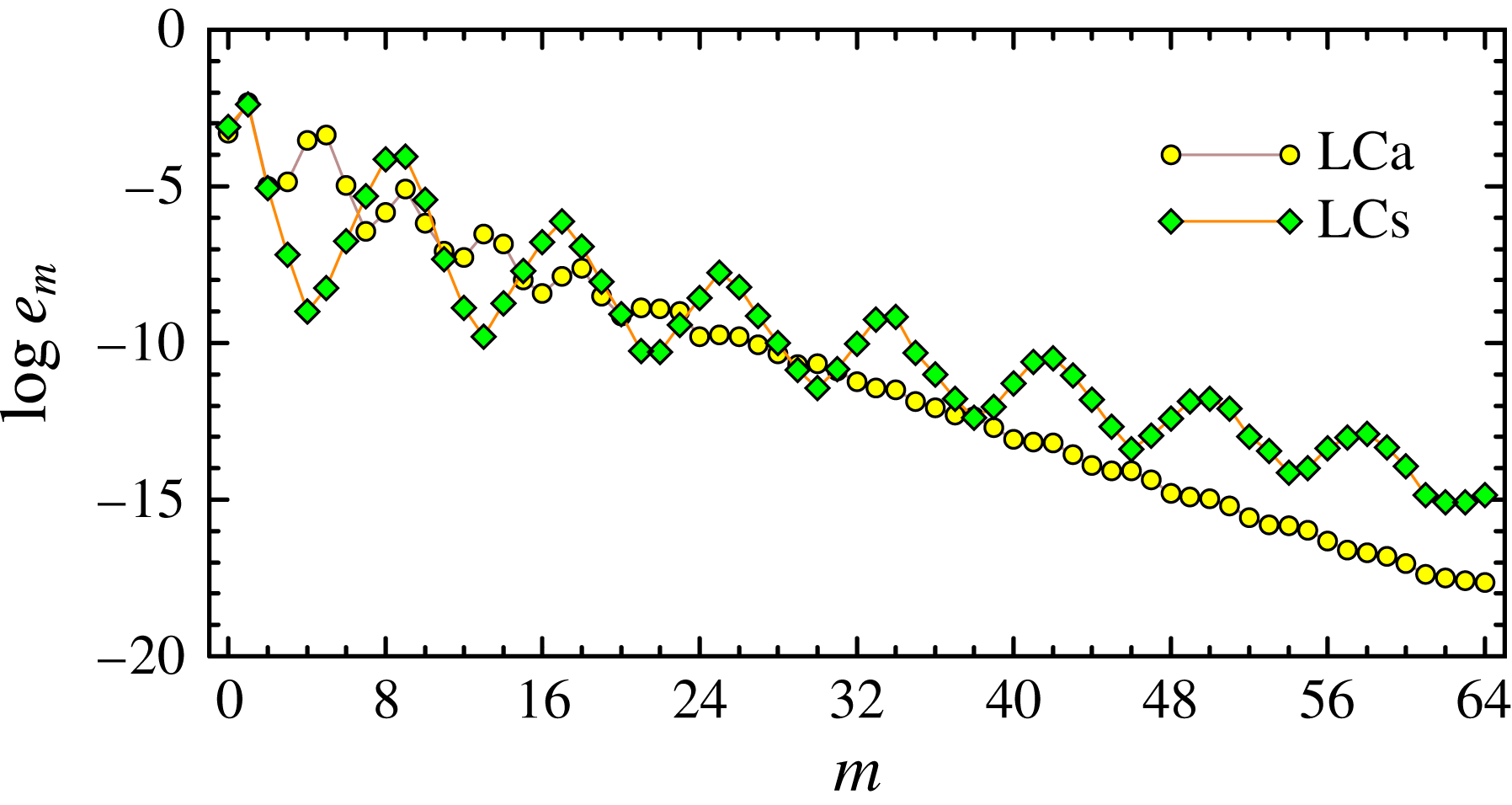
Relative modal kinetic energies,
 $e_{m}$
, of LCa at
 $\unicode[STIX]{x1D714}_{0}=4500$
and
 $Po=-0.3745$
(yellow circles) and LCs at
 $\unicode[STIX]{x1D714}_{0}=8000$
and
 $Po=-0.4$
(green diamonds).

Figure 5 shows that there are four helicity columns in LCa. Figure 6 shows the relative modal kinetic energies of LCa (filled yellow circles), and we indeed observe that, apart from
 $e_{0}$
and
 $e_{1}$
which are relative modal energies in the main azimuthal Fourier components of BS,
 $e_{4}$
and
 $e_{5}$
are larger than all the others by more than an order of magnitude. The figure also shows that the numerical solution LCa is well resolved. The presence of modal energies
 $e_{1}$
,
 $e_{4}$
and
 $e_{5}$
is suggestive of a triadic resonance. However, it cannot be a resonance between three Kelvin modes because the
 $(1,1,1)$
spatial structure associated with the overturning base flow BS is not a Kelvin mode, but a forced flow, as discussed earlier. However, it is still possible for two free Kelvin modes to resonate with the forced
 $(1,1,1)$
flow BS. In order to explore this possibility, we have plotted in figure 4(e–h) isosurfaces of the axial velocity of the azimuthal Fourier components
 $m=4$
and
 $m=5$
of LCa. As in the case of pure Kelvin modes (3.2), these Fourier components have a well-defined number of zeros in the radial, axial and azimuthal directions, and we can associate with them the integers
 $(k,m,n)$
, as is typically done with Kelvin modes. The sign of
 $m$
remains to be determined, and that depends on the sense of rotation of the Fourier components in the cylinder frame; positive
 $m$
corresponds to retrograde and negative
 $m$
corresponds to prograde rotation with respect to
 $\unicode[STIX]{x1D714}_{0}$
. In the table frame, both components have prograde rotation and their rotation frequencies are
 $\unicode[STIX]{x1D714}^{\mathit{drift}}=\unicode[STIX]{x1D714}_{\mathit{LCa}}/4=4854.13$
for
 $m=4$
and
 $\unicode[STIX]{x1D714}^{\mathit{drift}}=\unicode[STIX]{x1D714}_{\mathit{LCa}}/5=3883.30$
for
 $m=5$
. According to (3.6), the
 $m=4$
component rotates prograde (
 $\unicode[STIX]{x1D70E}^{\mathit{drift}}=354.13$
) and the
 $m=5$
component is retrograde (
 $\unicode[STIX]{x1D70E}^{\mathit{drift}}=-616.70$
) in the cylinder frame. The temporal frequencies in the cylinder frame (3.6) are given by
 $\unicode[STIX]{x1D70E}_{LCa,4}/\unicode[STIX]{x1D714}_{0}=0.3148$
for
 $m=4$
, and
 $\unicode[STIX]{x1D70E}_{LCa,5}/\unicode[STIX]{x1D714}_{0}=0.6852$
for
 $m=5$
. Therefore, their structure corresponds to modes
 $(1,-4,1)$
and
 $(1,5,2)$
. It is worth noting that
 $\unicode[STIX]{x1D70E}_{LCa,4}/\unicode[STIX]{x1D714}_{0}+\unicode[STIX]{x1D70E}_{LCa,5}/\unicode[STIX]{x1D714}_{0}=1$
, and hence the triadic resonance conditions between these two Fourier modes and the forced
 $(1,1,1)$
overturning flow BS are fulfilled exactly. This is because for a Hopf bifurcation there is only a single frequency in the table frame, so all the Fourier components have the same temporal frequency.
Now we compare the
 $m=4$
and
 $m=5$
azimuthal components of LCa with the Kelvin modes corresponding to the geometry (aspect ratio
 $\unicode[STIX]{x1D6E4}=1.33$
and tilt angle
 $\unicode[STIX]{x1D6FC}=3^{\circ }$
) and Poincaré number of LCa. The frequency of a Kelvin mode
 $K_{kmn}$
is given by (Marques & Lopez Reference Marques and Lopez2015):
 $$\begin{eqnarray}\frac{\unicode[STIX]{x1D70E}_{kmn}}{\unicode[STIX]{x1D714}_{0}}=\frac{2(1+Po\cos \unicode[STIX]{x1D6FC})}{\sqrt{1+(\unicode[STIX]{x1D6E4}a_{k}/n\unicode[STIX]{x03C0})^{2}}},\end{eqnarray}$$
where
 $a_{k}$
is given by (3.3). The spatial structure of
 $K_{kmn}$
and the angle
 $\unicode[STIX]{x1D6FD}$
of the characteristics depend only on the aspect ratio
 $\unicode[STIX]{x1D6E4}$
; the frequency
 $\unicode[STIX]{x1D70E}_{kmn}$
depends also on the tilt angle
 $\unicode[STIX]{x1D6FC}$
and Poincaré number
 $Po$
, because the axial angular velocity
 $\unicode[STIX]{x1D714}_{a}$
of the cylinder depends on them (2.6). We use the detuning parameter
 $\unicode[STIX]{x1D6FF}_{3}$
(3.12) to quantify how close a pair of free Kelvin modes are to a triadic resonance with the forced
 $(1,1,1)$
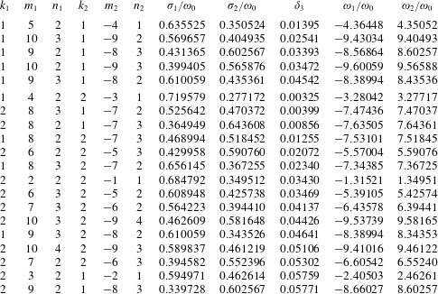
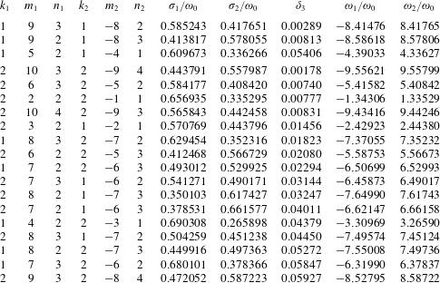
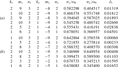
BS. Table 2 shows the pairs of Kelvin modes closest to resonance with BS, with detuning parameter
 $\unicode[STIX]{x1D6FF}_{3}<0.06$
, and with
 $k=1,2$
,
 $n\leqslant 4$
and
 $|m|\leqslant 10$
. The first section of the table corresponds to close resonances with
 $k=1$
. The closest resonance is precisely the
 $(1,-4,1)$
and
 $(1,5,2)$
case, consistent with the numerical solutions of the Navier–Stokes equations. Of course, the Kelvin modes
 $K_{1-41}$
and
 $K_{152}$
are not the same as the
 $m=4$
and
 $m=5$
azimuthal Fourier components of LCa. In particular, their structure near the walls, inside the boundary layers, is completely different because the Kelvin modes do not satisfy the physical no-slip boundary conditions. However, the inviscid Kelvin modes and the Fourier components of LCa are strikingly similar in the bulk, and moreover, the values of the frequencies
 $\unicode[STIX]{x1D70E}$
are also very close:
 $$\begin{eqnarray}\frac{\unicode[STIX]{x1D70E}_{LCa,4}}{\unicode[STIX]{x1D714}_{0}}=0.3148,\frac{\unicode[STIX]{x1D70E}_{1-41}^{K}}{\unicode[STIX]{x1D714}_{0}}=0.3505;\quad \text{and}\quad \frac{\unicode[STIX]{x1D70E}_{LCa,5}}{\unicode[STIX]{x1D714}_{0}}=0.6852,\frac{\unicode[STIX]{x1D70E}_{152}^{K}}{\unicode[STIX]{x1D714}_{0}}=0.6355.\end{eqnarray}$$
The last two columns in table 2 show the frequencies of the Kelvin modes in the table frame. Apart from the sign, they are very close to the temporal frequency of LCa,
 $\unicode[STIX]{x1D714}_{\mathit{LCa}}/\unicode[STIX]{x1D714}_{0}=4.315$
. The sign of
 $\unicode[STIX]{x1D714}$
in the last two columns, together with
 $m$
, determines the azimuthal drift of the Kelvin modes in the table frame (3.6), and both are prograde, as are the
 $m=4$
and
 $m=5$
Fourier modes of LCa. Furthermore,
 $K_{1-41}$
and
 $K_{152}$
are not
 ${\mathcal{I}}$
symmetric because
 $m+n$
is odd (3.7). This is consistent with the
 ${\mathcal{I}}$
symmetry being broken at the Hopf bifurcation. We know that when
 $m+n$
is odd, the Kelvin modes have a spatio-temporal symmetry (3.9), and this is precisely the symmetry of LCa (see the earlier discussion of figure 5). All of this strongly suggests that at the Hopf bifurcation spawning LCa, a triadic resonance between the forced
 $(1,1,1)$
flow BS and the free Kelvin modes
 $K_{1-41}$
and
 $K_{152}$
is excited, resulting in the instability of BS.
 $K_{1-41}$
and
 $K_{152}$
are not exactly tuned to a perfect triadic resonance, but are very close to resonance, with a detuning of only 1.4 %.
Kelvin mode pairs,
 $K_{k_{1}m_{1}n_{1}}$
and
 $K_{k_{2}m_{2}n_{2}}$
, closest to resonance with the forced
 $(1,1,1)$
mode for
 $\unicode[STIX]{x1D6E4}=1.33$
,
 $\unicode[STIX]{x1D6FC}=3^{\circ }$
and
 $Po=-0.3745$
, for
 $k\leqslant 2$
,
 $n\leqslant 4$
and
 $m\leqslant 10$
, and detuning
 $\unicode[STIX]{x1D6FF}_{3}<0.06$
.
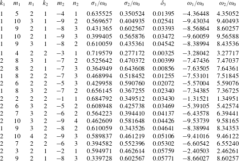
The presence of a triadic resonance is not surprising, because there are many pairs of Kelvin modes with small detuning
 $\unicode[STIX]{x1D6FF}_{3}$
. By fixing
 $k=1$
and
 $\unicode[STIX]{x1D6FF}_{3}<0.06$
there is not only the 1 :
 $-4$
: 5 resonance, but also four additional pairs with
 $|m|\in [8,10]$
. If the
 $k=1$
condition is relaxed to
 $k\leqslant 2$
, 15 additional pairs appear, some of them with smaller detuning parameter values than in the 1 :
 $-4$
: 5 case, as shown in table 2. Considering larger values of
 $k$
,
 $m$
and
 $n$
identifies more pairs, many of them with arbitrarily small detuning
 $\unicode[STIX]{x1D6FF}_{3}$
. This is because the Kelvin mode frequencies are dense (Greenspan Reference Greenspan1968). However, these Kelvin modes with large values of
 $k$
,
 $m$
and
 $n$
are quickly damped by viscosity (Greenspan Reference Greenspan1968), and so they are not expected to play any significant dynamical role. It is worth noting that the instability mechanism at the Hopf bifurcation is not given by the closest-to-resonance pair of Kelvin modes (the pair with the minimum value of the detuning parameter). The detuning must be small in order to have resonance, but other factors may play a critical role in the selection, for example the presence or absence of retracing rays, the boundary layer structure, the nonlinearities in the forced
 $(1,1,1)$
BS, the damping and detuning effects of viscosity, imperfections and noise. The list of possibilities is long, and the only way to decide which resonances will destabilize the base state is to (numerically) solve the Navier–Stokes equations with no-slip boundary conditions. Considering the detuning parameter alone is very limited and does not allow one to discriminate which of the possible resonances will play a role, except perhaps when the geometry and Poincaré number are fine-tuned to a specific low-order (with moderate values of
 $k$
,
 $|m|$
and
 $n$
) triadic resonance (e.g. as was done in Lagrange et al.
Reference Lagrange, Meunier, Nadal and Eloy2011; Albrecht et al.
Reference Albrecht, Blackburn, Lopez, Manasseh and Meunier2015; Marques & Lopez Reference Marques and Lopez2015; Lopez & Marques Reference Lopez and Marques2016b
).
In order to determine if the second group of potential resonances centred around
 $|m|=9$
play any role in the present problem, we have computed the unstable BS for
 $\unicode[STIX]{x1D714}_{0}>3992$
(the critical
 $\unicode[STIX]{x1D714}_{0}$
at which BS become unstable to LCa). We have computed these unstable basic states by restricting the computation to the
 ${\mathcal{I}}$
-symmetric subspace. This strategy works until BS become unstable in the symmetric subspace at
 $\unicode[STIX]{x1D714}_{0}\approx 7000$
, where it loses stability at a secondary Hopf bifurcation. The unstable BS is then computed beyond this bifurcation point by using the selective-frequency-damping method (Äkervik et al.
Reference Äkervik, Brandt, Henningson, Hœpffner, Marxen and Schlatter2006), which suppresses the oscillations of the bifurcated solution and drives the simulation toward the unstable BS.
For unstable LCs (computed in the
 ${\mathcal{I}}$
-subspace), at
 $\unicode[STIX]{x1D714}_{0}=7000$
and
 $Po=-0.3745$
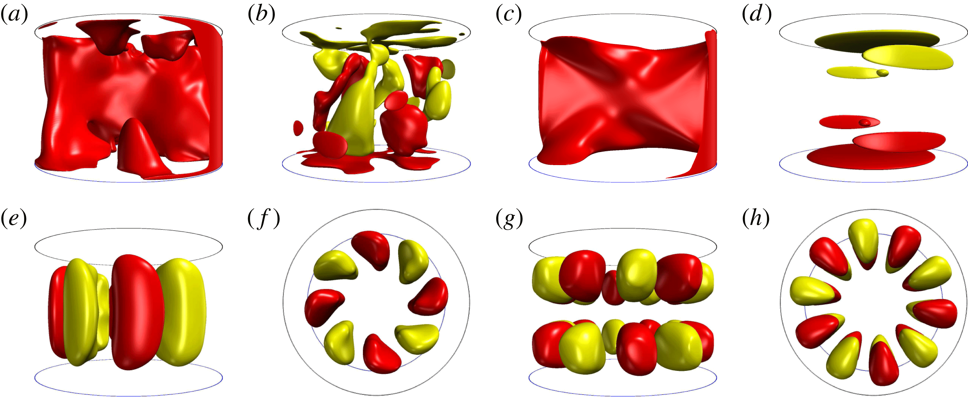
, shown are isosurfaces of (a)
 $w=2$
and (b)
 ${\mathcal{H}}=\pm 5\times 10^{5}$
, and of the (unstable) BS at the same parameters (computed in the
 ${\mathcal{I}}$
-symmetric subspace; the bifurcation of LCs from BS in the subspace is slightly subcritical, such that both BS and LCs are stable at
 $\unicode[STIX]{x1D714}_{0}=7000$
in the subspace), with (c)
 $w=2$
and (d)
 ${\mathcal{H}}=\pm 5\times 10^{5}$
. The supplementary movie shows an animation of
 ${\mathcal{H}}$
for LCs over one period
 $\unicode[STIX]{x1D70F}_{\mathit{LCs}}=9.50\times 10^{-5}$
. Isosurfaces of the (e,f)
 $m=8$
and (g,h)
 $m=9$
azimuthal Fourier components of
 $w$
at levels
 $w=\pm 30$
are shown in two orthogonal views.

The structure of the solution that bifurcates at the second Hopf bifurcation of BS is a symmetric limit cycle LCs (an
 $F$
-cyle), shown in figure 7(a,b) for
 $\unicode[STIX]{x1D714}_{0}=7000$
(close to the bifurcation point). Also plotted in figure 7(c,d) is the structure of the unstable BS at the same point in parameter space, computed using the selective-frequency-damping method (Äkervik et al.
Reference Äkervik, Brandt, Henningson, Hœpffner, Marxen and Schlatter2006). The
 $w$
isosurface of LCs resembles that of BS, but it is distorted by small structures approximately one third the cylinder height in size. The corresponding helicity isosurfaces for LCs show the presence of helical structures in the bulk, but instead of columns these are also structures whose size is also approximately one third of the cylinder height. These structures are absent in BS. The helical structures, and their temporal evolution, can be appreciated in the supplementary online movie: they rotate prograde and undergo significant distortions during the period of the solution, with frequency
 $\unicode[STIX]{x1D714}_{s}=66\,139$
. Figure 6 shows the relative modal kinetic energies of LCs (filled green diamonds). Apart from
 $e_{0}$
and
 $e_{1}$
which are the modal energies of the main components of BS,
 $e_{8}$
and
 $e_{9}$
are larger than all the other modal energies by more than an order of magnitude. The figure also shows that LCs is numerically well resolved. The presence of dominant
 $e_{1}$
,
 $e_{8}$
and
 $e_{9}$
is again suggestive of a triadic resonance. In order to explore this possibility, we have plotted isosurfaces of the axial velocity for the
 $m=8$
and
 $m=9$
azimuthal Fourier components of LCs in figure 7(e–h). Their spatial structures in the bulk are the same as for Kelvin eigenmodes
 $K_{1,\pm 8,2}$
and
 $K_{1,\pm 9,3}$
; the sign of the azimuthal number
 $m$
remains to be determined. The only pair of Kelvin modes in the first part of table 2 with this spatial structure indicates that the system is close to a triadic resonance between the forced
 $(1,1,1)$
BS,
 $K_{1-82}$
and
 $K_{193}$
. The signs of
 $\unicode[STIX]{x1D714}$
in the last two columns of the table and of
 $m$
, indicate that these two Kelvin modes are prograde in the table frame, and that they are both
 ${\mathcal{I}}$
symmetric (
 $m+n$
is even), as is the computed LCs. The only discrepancy is in the temporal frequencies in the table frame; for the Kelvin modes the frequency would be approximately 8.4, while the computed frequency of LCs is
 $\unicode[STIX]{x1D714}_{\mathit{LCs}}/\unicode[STIX]{x1D714}_{0}=9.45$
. This discrepancy of approximately 10 % is of the order of magnitude of the detuning, approximately 4.5 %. Of course,
 $K_{1-82}$
and
 $K_{193}$
are not the same as the
 $m=8$
and
 $m=9$
azimuthal Fourier components of LCs; boundary layers, viscosity and nonlinearities account for the differences between them. It is worth noting that, as in the 1 :
 $-4$
: 5 resonance of LCa, the instability mechanism at the Hopf bifurcation of LCs is not determined by the closest-to-resonance pair of free Kelvin modes.
5.2 The
$Po=-0.4$
case (retracing rays)

The change in
 $Po$
from
 $Po=-0.3745$
(non-retracing rays) to
 $Po=-0.4$
(retracing rays), results in a dramatic change in the states and instabilities encountered as
 $\unicode[STIX]{x1D714}_{0}$
is increased, as illustrated in figure 3. There are three main differences between the two
 $Po$
scenarios. The first is that in the retracing rays scenario, BS is stable to much larger
 $\unicode[STIX]{x1D714}_{0}$
values: BS becomes unstable at
 $\unicode[STIX]{x1D714}_{0}\approx 7240$
, approximately 80 % larger than the critical value at
 $Po=-0.3745$
,
 $\unicode[STIX]{x1D714}_{0}\approx 3992$
. The second difference is that the stable bifurcated state is LCs, an
 ${\mathcal{I}}$
-symmetric limit cycle, instead of being LCa. Moreover, in the non-retracing rays scenario, LCs was never stable, and it had to be computed by restricting the simulations to the
 ${\mathcal{I}}$
-symmetric subspace. Finally, the third main difference is that the asymmetric branch with LCa, and more complex states, QPa and VLFa (to be described later), still exists but is not connected (via stable states) to BS, and it has shifted to much larger values of
 $\unicode[STIX]{x1D714}_{0}$
. For
 $Po=-0.4$
, the LCa branch starts at
 $\unicode[STIX]{x1D714}_{0}\approx 6800$
, while for
 $Po=-0.3745$
it starts at
 $\unicode[STIX]{x1D714}_{0}\approx 3992$
.
For LCs at
 $\unicode[STIX]{x1D714}_{0}=8000$
and
 $Po=-0.4$
, shown are isosurfaces of (a)
 $w=2$
and (b)
 ${\mathcal{H}}=\pm 5\times 10^{5}$
, and of (unstable) BS at the same parameters (computed using selective-frequency damping) with (c)
 $w=2$
and (d)
 ${\mathcal{H}}=\pm 5\times 10^{5}$
. The supplementary movie shows an animation of
 ${\mathcal{H}}$
for LCs over one period
 $\unicode[STIX]{x1D70F}_{\mathit{LCs}}=9.36\times 10^{-5}$
. Isosurfaces of the (e,f)
 $m=8$
and (g,h)
 $m=9$
azimuthal Fourier components of
 $w$
at levels
 $w=\pm 30$
are shown in two orthogonal views.

Kelvin mode pairs,
 $K_{k_{1}m_{1}n_{1}}$
and
 $K_{k_{2}m_{2}n_{2}}$
, closest to resonance with the forced
 $(1,1,1)$
mode for
 $\unicode[STIX]{x1D6E4}=1.33$
,
 $\unicode[STIX]{x1D6FC}=3^{\circ }$
and
 $Po=-0.4$
, for
 $k\leqslant 2$
,
 $n\leqslant 4$
and
 $m\leqslant 10$
, and detuning
 $\unicode[STIX]{x1D6FF}<0.06$
.
The structure of LCs at
 $Po=-0.4$
is shown in figure 8 for
 $\unicode[STIX]{x1D714}_{0}=8000$
. Figure 8(a–d) shows isosurfaces of axial velocity
 $w$
and helicity
 ${\mathcal{H}}$
of LCs, and the corresponding isosurfaces for BS at the same parameter values (computed using selective-frequency damping as BS is unstable even in the
 ${\mathcal{I}}$
-symmetric subspace). Comparing with LCs at
 $Po=-0.3745$
and
 $\unicode[STIX]{x1D714}_{0}=7000$
in figure 7, we observe that the inertial beams emerging from the corner in the basic state BS are much more clearly defined than in the
 $Po=-0.3745$
case. The structure of the
 $m=8$
and
 $m=9$
azimuthal Fourier modes is very similar to the structure of the same Fourier modes in the
 $Po=-0.3745$
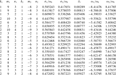
branch. In order to see if the triadic resonance 1:-8:9 is the instability mechanism for the Hopf bifurcation where the stable LCs is spawned, we have computed the pairs of Kelvin modes closest to resonance with the forced BS, with detuning parameter
 $\unicode[STIX]{x1D6FF}_{3}<0.06$
, and with
 $k=1,2$
,
 $n\leqslant 4$
and
 $|m|\leqslant 10$
for
 $Po=-0.4$
(the results are presented in table 3). By comparing with table 2, and focusing on the
 $k=1$
cases in the first section of each table, we find that the pair of Kelvin modes closest to resonance with the forced BS is now
 $K_{1-82}$
and
 $K_{193}$
(
 $\unicode[STIX]{x1D6FF}_{3}\approx 0.003$
), while the pair
 $K_{1-41}$
and
 $K_{152}$
associated with the triadic resonance leading to LCa in the
 $Po=-0.3745$
case, has moved now to third position, with a detuning that is 18 times larger (
 $\unicode[STIX]{x1D6FF}_{3}\approx 0.054$
). This example shows how a small variation in the Poincaré number (6 % from
 $Po=-0.3745$
to
 $-0.4$
) results in dramatic changes in the detuning parameter of close-to-resonance pairs of Kelvin modes. In this case, the changes in detuning result in different triadic resonances at the first Hopf bifurcation of BS: 1 :
 $-4$
: 5, which breaks the
 ${\mathcal{I}}$
symmetry, for
 $Po=-0.3745$
, and 1 :
 $-8$
: 9, which preserves the
 ${\mathcal{I}}$
symmetry, for
 $Po=-0.4$
. The second section of table 3 shows the additional close-to-resonance pairs with
 $\unicode[STIX]{x1D6FF}_{3}<0.6$
when we relax the
 $k$
values to
 $k\leqslant 2$
. Again, 15 additional Kelvin eigenmode pairs appear with some of them having a smaller detuning parameter value than the 1 :
 $-8$
: 9 case.
For LCa at
 $\unicode[STIX]{x1D714}_{0}=6800$
and
 $Po=-0.4$
, shown are isosurfaces of (a)
 $w=2$
and (b)
 ${\mathcal{H}}=\pm 8\times 10^{5}$
, and of the (stable) BS at the same parameters with (c)
 $w=2$
and (d)
 ${\mathcal{H}}=\pm 4\times 10^{5}$
. The supplementary movie shows an animation of
 ${\mathcal{H}}$
for LCa over one period
 $\unicode[STIX]{x1D70F}_{\mathit{LCs}}=2.15\times 10^{-4}$
. Isosurfaces of the (e,f)
 $m=4$
and (g,h)
 $m=5$
azimuthal Fourier components of
 $w$
at levels
 $w=\pm 90$
are shown in two orthogonal views.

As shown in figure 3, the asymmetric branch with LCa, QPa and VLFa also exists for
 $Po=-0.4$
. The structure of LCa is shown in figure 9 for
 $\unicode[STIX]{x1D714}_{0}=6800$
. Comparing with LCa at
 $Po=-0.3745$
and
 $\unicode[STIX]{x1D714}_{0}=4500$
in figure 4, we observe that the inertial beams emerging from the corner in BS are much more clearly defined than in the
 $Po=-0.3745$
case. The spatial structure of the
 $m=4$
and
 $m=5$
azimuthal Fourier modes is the same in the two cases
 $Po=-0.3745$
and
 $Po=-0.4$
, with quantitative differences due to the large difference in
 $\unicode[STIX]{x1D714}_{0}$
for the two examples. The first section of table 3 shows that the resonance 1 :
 $-4$
: 5 also has a small detuning in the
 $Po=-0.4$
, and therefore it is very likely to be the triadic resonance that explains the features of LCa on the disconnected asymmetric branch for
 $Po=-0.4$
.
6 Subsequent instabilities
The amplitude of the precessional forcing is given by
 $\unicode[STIX]{x1D714}_{p}\sin \unicode[STIX]{x1D6FC}=\unicode[STIX]{x1D714}_{0}Po\sin \unicode[STIX]{x1D6FC}$
. Increasing
 $\unicode[STIX]{x1D714}_{0}$
, while keeping
 $Po$
and the geometry fixed, increases the forcing. This results in a relative reduction of the viscous effects and at the same time increases the importance of the nonlinear terms. In this section, we investigate what happens when
 $\unicode[STIX]{x1D714}_{0}$
is increased above the level discussed in the previous section, exploring the transitions from the limit cycle behaviours to more complex flows.
6.1 Asymmetric branch at
$Po=-0.3745$

Variation of (a)
 $e_{0}$
and (b)
 $S$
with
 $\unicode[STIX]{x1D714}_{0}$
, for the states as indicated (see table 1 for details of these states), for
 $Po=-0.3745$
.

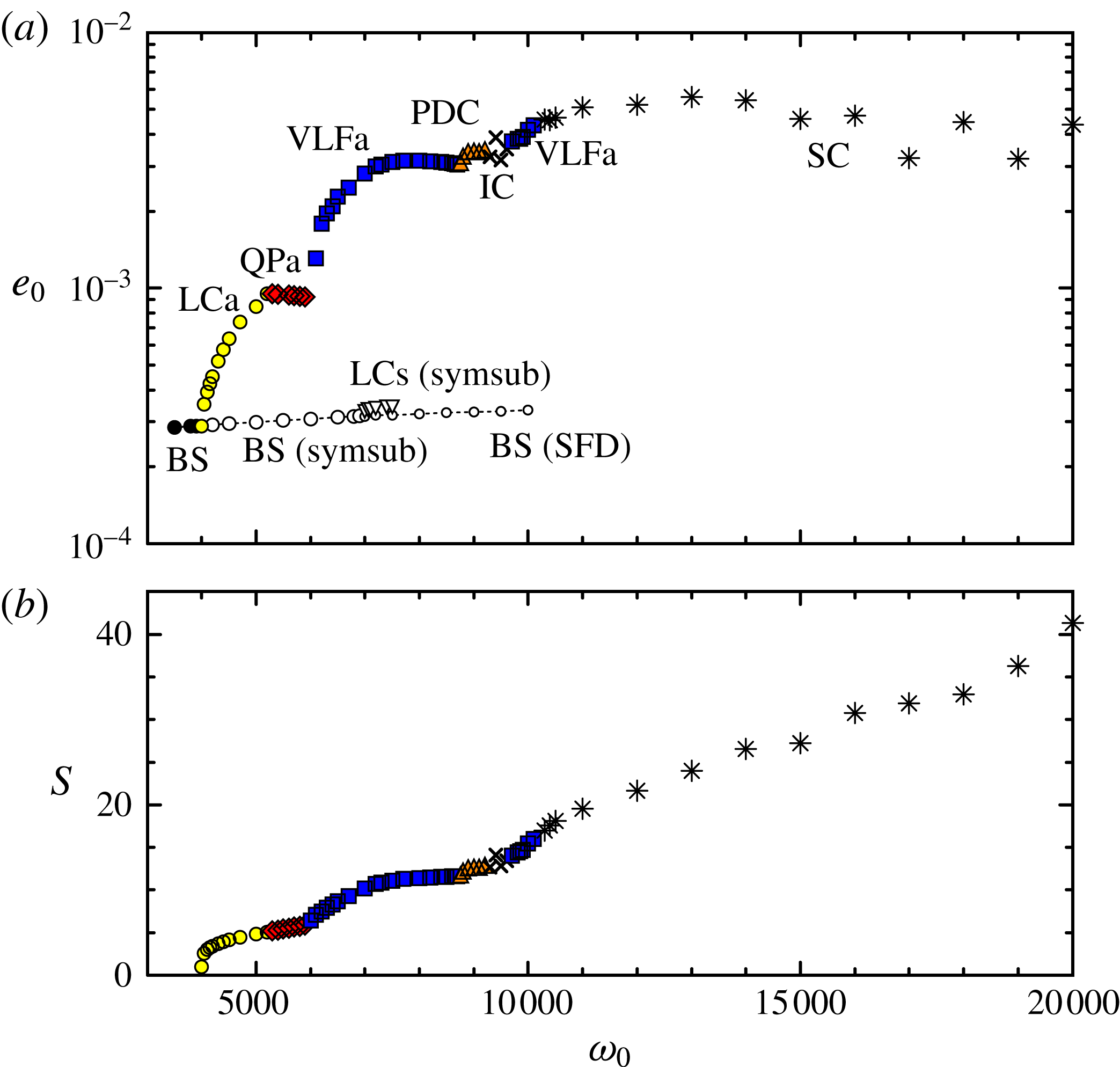
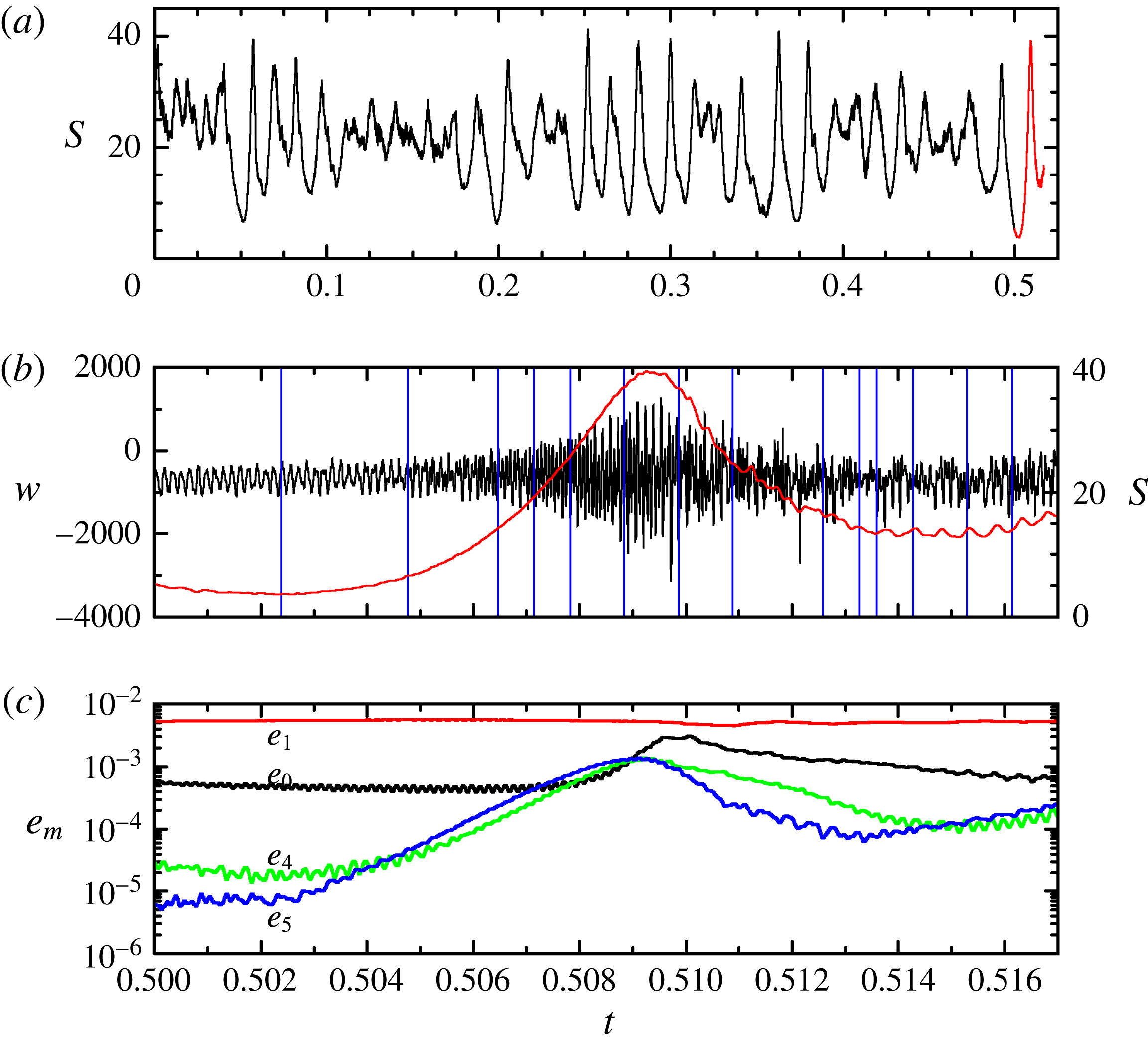
Figure 10 shows the variety of states, characterized by the relative azimuthally averaged kinetic energy
 $e_{0}$
and symmetry parameter
 $S$
, for
 $Po=-0.3745$
as
 $\unicode[STIX]{x1D714}_{0}$
is increased up to 20 000. The succession of states and their instabilities share many of the characteristics observed in previous simulations of the transition from the base state (BS) to sustained chaos (SC) (Marques & Lopez Reference Marques and Lopez2015; Lopez & Marques Reference Lopez and Marques2016b
). As detailed in § 5.1, BS first loses stability via a supercritical Hopf bifurcation that breaks the
 ${\mathcal{I}}$
symmetry, resulting in a (spatio-temporal)
 ${\mathcal{I}}^{st}$
-symmetric limit cycle LCa, whose spatio-temporal characteristics are consistent with a triadic resonance between BS and two free Kelvin modes,
 $K_{1-41}$
and
 $K_{152}$
. Further increasing
 $\unicode[STIX]{x1D714}_{0}$
, LCa becomes unstable at a Neimark–Sacker bifurcation that is not associated with any new triadic resonances, but corresponds to radial oscillations of the axisymmetric azimuthal mean flow induced by nonlinearities at the higher
 $\unicode[STIX]{x1D714}_{0}$
(Marques & Lopez Reference Marques and Lopez2015). This
 $m=0$
streaming flow is not a geostrophic component of the flow; the presence of wave beams generated by the boundary layers introduces an explicit axial variation in the streaming flow, irrespective of whether the beams are retracing or not. The quasiperiodic state spawned at the Neimark–Sacker bifurcation, QPa, loses stability at higher
 $\unicode[STIX]{x1D714}_{0}$
to a very-low-frequency three-torus state, VLFa. This bifurcation introduces an additional very low frequency. This third frequency is associated with the exchange of energy between the resonant
 $m=4$
and
 $m=5$
azimuthal Fourier components and the
 $m=0$
streaming flow component, and corresponds to recurrent excursions between some of the states obtained in the first bifurcations (BS, LCa and QPa), which are now all unstable. These unstable states only have a small number of unstable directions, and the VLFa flows are trajectories in phase space that are close to heteroclinic orbits between some of these saddle states. In the range
 $\unicode[STIX]{x1D714}_{0}\in [8400,8800]$
, a sequence of period doubling bifurcations (PDC) of VLFa states is then followed by a short interval in
 $\unicode[STIX]{x1D714}_{0}$
with intermittent chaotic (IC) states, and then the flow returns to VLFa solutions for
 $\unicode[STIX]{x1D714}_{0}\sim 10^{4}$
.
For the sustained chaos (SC) state
 $\unicode[STIX]{x1D714}_{0}=2\times 10^{4}$
and
 $Po=-0.3745$
, (a) shows the time series of
 $S$
over more than half a viscous time; (b,c) show details over
 $t\in [0.500,0.517]$
of axial velocity at
 $(r,\unicode[STIX]{x1D703},z)=(0.5,0,-\unicode[STIX]{x1D6E4}/4)$
,
 $S$
, and the leading relative modal energies
 $e_{m}$
. The blue vertical lines in (b) indicate the times corresponding to the snapshots of
 ${\mathcal{H}}$
shown in figure 12.

Snapshots of the helicity at isolevel
 ${\mathcal{H}}=\pm 9\times 10^{6}$
, at times as indicated, of SC at
 $\unicode[STIX]{x1D714}_{0}=2\times 10^{4}$
and
 $Po=-0.3745$
. See the supplementary movie for an animation of 101 snapshots at times uniformly spaced in the interval
 $t\in [0.500,0.517]$
.

For
 $\unicode[STIX]{x1D714}_{0}>10\,400$
, the flow transitions from VLFa to sustained chaos (SC). These states are chaotic trajectories with slow drifts in phase space between the different unstable saddle states, in the same way as in VLFa, but now at the higher
 $\unicode[STIX]{x1D714}_{0}$
, the transverse intersections between the stable and unstable manifolds of the saddle states are much more prominent, leading to heteroclinic chaos (Guckenheimer & Holmes Reference Guckenheimer and Holmes1997; Guckenheimer et al.
Reference Guckenheimer, Krauskopf, Osinga and Sandstede2015). This type of dynamics is consistent with the experimental observation by McEwan (Reference McEwan1970) and Manasseh (Reference Manasseh1992) of resonant collapse. Figure 11(a) shows the time series over more than half a viscous time of the symmetry parameter
 $S$
, which is chaotic but with well-defined spikes, for a solution at
 $\unicode[STIX]{x1D714}_{0}=2\times 10^{4}$
. One of the spikes is described in detail in figure 11(b), which shows time series of
 $S$
(again) together with the axial velocity at a point
 $w(r=0.5,\unicode[STIX]{x1D703}=0,z=-\unicode[STIX]{x1D6E4}/4,t)$
for
 $t\in [0.500,0.517]$
, corresponding to the last spike shown in red in figure 11(a). Figure 11(c) shows time series of the dominant modal energies involved around the spike. The now unstable LCa, which was spawned at the 1 :
 $-4$
: 5 triadic resonance-induced Hopf bifurcation, is visited for a short time and then the flow collapses to a chaotic state. This process is illustrated in figure 12, showing 15 snapshots of helicity isosurfaces at various times indicated by the blue vertical lines in figure 11(b); the supplementary movie further illustrates this resonant collapse behaviour which consists of 101 snapshots of the helicity
 ${\mathcal{H}}$
at uniformly spaced times in the interval
 $t\in [0.500,0.517]$
. Note that there is much going on at very disparate time scales, and the movie is far from being smooth; it would need one or two orders of magnitude more frames and this is prohibitively large to include online. The LCa state with the well-defined helical columns of the 1 :
 $-4$
: 5 resonance is clearly visible in figure 12(f). Then, in figure 12(i,j) the flow becomes chaotic, developing small-scale structures throughout, leading to the detuning characterized by the spike in
 $e_{0}$
(figure 11
c), and then it collapses in figure 12(n) as the large
 $e_{0}$
drives the system away (detunes) from the support for the 1 :
 $-4$
: 5 resonance.
6.2 Symmetric and asymmetric branches at
$Po=-0.4$

Variation of (a)
 $e_{0}$
and (b)
 $S$
, for the states as indicated, with
 $\unicode[STIX]{x1D714}_{0}$
, for
 $Po=-0.4$
.

Figure 13 shows what happens at
 $Po=-0.4$
as
 $\unicode[STIX]{x1D714}_{0}$
is increased. As detailed in § 5.2, LCs is the first state to bifurcate from BS in a supercritical Hopf bifurcation that preserves the
 ${\mathcal{I}}$
symmetry, and the limit cycle that is spawned, LCs, has spatio-temporal structure consistent with a triadic resonance between BS and two free Kelvin modes
 $K_{1-82}$
and
 $K_{193}$
. At
 $\unicode[STIX]{x1D714}_{0}\approx 8460$
, LCs becomes unstable, and the flow jumps to a remote solution VLFa on the asymmetric branch. The most likely scenario from dynamical systems theory is that LCs undergoes a subcritical Neimark–Sacker bifurcation that breaks
 ${\mathcal{I}}$
symmetry, and as the bifurcated solutions are unstable, the flow evolves to another stable state that is remote in phase space. The unstable LCs branch, that continues to exist past the Neimark–Sacker bifurcation, can be continued to higher
 $\unicode[STIX]{x1D714}_{0}$
in the
 ${\mathcal{I}}$
-invariant subspace, as shown in figure 13. The
 ${\mathcal{I}}$
-symmetric LCs exhibiting the 1 :
 $-8$
: 9 resonance exists and is stable in the range
 $\unicode[STIX]{x1D714}_{0}\in [7240,8460]$
. For
 $\unicode[STIX]{x1D714}_{0}>8460$
we have not found any stable
 ${\mathcal{I}}$
-symmetric solution, and the only stable branch of solutions is the asymmetric branch, associated with the triadic resonance 1 :
 $-4$
: 5.
Temporal evolution of axial velocity
 $w(0.5,0,-\unicode[STIX]{x1D6E4}/2,t)$
(blue) and
 $S$
(red), for a simulation at
 $\unicode[STIX]{x1D714}_{0}=8650$
starting with the LCs state at
 $\unicode[STIX]{x1D714}_{0}=8450$
as the initial condition.

Figure 14 shows the time series of the axial velocity at a point,
 $w(0.5,0,-\unicode[STIX]{x1D6E4}/2,t)$
(shown in black) along with the symmetry parameter
 $S$
(shown in red), for a simulation at
 $\unicode[STIX]{x1D714}_{0}=8650$
starting with the LCs state at
 $\unicode[STIX]{x1D714}_{0}=8450$
as the initial condition. The flow appears to have settled early on (within approximately 0.14 viscous times) to an LCs state that seems stable for about the first viscous time. One viscous time corresponds to
 $\unicode[STIX]{x1D714}_{0}/2\unicode[STIX]{x03C0}$
cylinder rotations; for
 $\unicode[STIX]{x1D714}_{0}=8650$
this is approximately 1377 cylinder rotations. The 0.14 viscous time corresponds to
 $0.14\unicode[STIX]{x1D714}_{0}/2\unicode[STIX]{x03C0}\approx 190$
cylinder rotations, and this is approximately the Ekman spin-up time
 $1/\sqrt{Ek}=\sqrt{4\unicode[STIX]{x1D714}_{0}}$
. However, by monitoring its symmetry, we see that
 $S$
is growing exponentially during this time. By
 $t\approx 1$
,
 $S\approx 10^{-2}$
, and the flow is seen to transition to another state which is quasi-periodic of QPa type with
 $S\approx 3$
. This state itself is unstable, and at
 $t\approx 2.3$
, there is another transition to a very-low-frequency VLFa state, which is also unstable, and at
 $t\approx 2.7$
there is another transition to another VLFa which appears to be stable; we have tracked it for over 2 viscous times (about 3000 cylinder rotations) without any further transitions. This type of evolution in a hysteretic regime is quite common, with the transitory evolution being attracted to unstable saddle states along their stable manifolds only to be diverted away along their unstable manifolds. Very similar behaviour is found in the hysteresis regime of the cubic lid-driven cavity flow (Lopez et al.
Reference Lopez, Welfert, Wu and Yalim2017). The stable VLFa solution that was obtained can be continued to lower
 $\unicode[STIX]{x1D714}_{0}$
, and undergoes a very similar sequence of bifurcations as in the asymmetric branch for
 $Po=-0.3745$
. At about
 $\unicode[STIX]{x1D714}_{0}\approx 6800$
, the LCa limit cycle becomes unstable in a cyclic-fold bifurcation (a saddle-node bifurcation of limit cycles), and the flow jumps back to BS for lower
 $\unicode[STIX]{x1D714}_{0}$
. This is a large hysteretic loop between the symmetric and asymmetric solution branches, covering
 $\unicode[STIX]{x1D714}_{0}\in [6800,8460]$
. Similar hysteretic behaviour in a precessing cylinder experiment has been reported by Herault et al. (Reference Herault, Gundrum, Giesecke and Stefani2015) who fixed
 $\unicode[STIX]{x1D714}_{0}\sim 5\times 10^{5}$
and varied
 $Po\in [0,0.15]$
in a cylinder of aspect ratio
 $\unicode[STIX]{x1D6E4}=2$
at tilt angle
 $\unicode[STIX]{x1D6FC}=90^{\circ }$
.
Power spectral density (PSD) of
 $w$
at the point
 $(r,\unicode[STIX]{x1D703},z)=(0.5,0,-\unicode[STIX]{x1D6E4}/4)$
with
 $Po=-0.4$
for the states (a) LCa at
 $\unicode[STIX]{x1D714}_{0}=6800$
, (b) QPa at
 $\unicode[STIX]{x1D714}_{0}=7250$
, (c) VLFa at
 $\unicode[STIX]{x1D714}_{0}=8650$
, and (d) SC at
 $\unicode[STIX]{x1D714}_{0}=20\,000$
.

Phase portraits and Poincaré sections of QPa.

For the various types of solutions obtained with
 $Po=-0.4$
, figure 15 shows the power spectral density (PSD) of the axial velocity
 $w$
at the point
 $(r,\unicode[STIX]{x1D703},z)=(0.5,0,-\unicode[STIX]{x1D6E4}/4)$
. The PSD are plotted in logarithmic scale because the relevant frequencies cover more than three orders of magnitude. Figure 15(a) shows the PSD of the
 ${\mathcal{I}}^{st}$
-symmetric limit cycle LCa, with a fundamental frequency
 $f_{1}=\unicode[STIX]{x1D714}_{\mathit{LCa}}/\unicode[STIX]{x1D714}_{0}=4.2977$
plus higher harmonics. The PSD of the quasi-periodic QPa is shown in figure 15(b). There are three large-amplitude peaks at frequencies
 $f_{1}=4.3144$
,
 $f_{2}=2.3060$
and
 $f_{3}=2.0084$
and another one at frequency
 $f_{4}=0.2976$
, which is approximately an order of magnitude smaller than
 $f_{1}=\unicode[STIX]{x1D714}_{\mathit{LCa}}/\unicode[STIX]{x1D714}_{0}$
. These frequencies are linearly related,
 $f_{3}=f_{1}-f_{2}$
and
 $f_{4}=2f_{2}-f_{1}$
. The frequencies of all the peaks in figure 15(b) are linear combinations of the two frequencies with largest amplitudes,
 $f_{1}$
and
 $f_{2}$
, and so QPa is a two-torus. Figure 16(a,b) shows phase portraits of LCa and QPa, where the two-torus structure of QPa is clearly seen. The variables used to illustrate these two views of the phase portraits are the axial velocities at three different points:
 $w_{1}=w(0.5,0,-\unicode[STIX]{x1D6E4}/4,t)$
,
 $w_{2}=w(0.5,\unicode[STIX]{x03C0},\unicode[STIX]{x1D6E4}/4,t)$
, and
 $w_{3}=w(0.5,\unicode[STIX]{x03C0},-\unicode[STIX]{x1D6E4}/4,t)$
. The points in the cylinder corresponding to
 $w_{1}$
and
 $w_{2}$
are
 ${\mathcal{I}}$
-related. Figure 16(a), the phase portrait using the
 ${\mathcal{I}}$
-related
 $w_{1}$
and
 $w_{2}$
shows that LCa and QPa are setwise symmetric; in the variables used,
 ${\mathcal{I}}$
-symmetry means reflection symmetry with respect to the line
 $w_{1}+w_{2}=0$
(the grey line in figure 16
a). If LCa and QPa were pointwise
 ${\mathcal{I}}$
-symmetric, they would be contained onto the line
 $w_{1}+w_{2}=0$
. In figure 16(a), the phase portrait of LCa has been translated along the symmetry line
 $w_{1}+w_{2}=0$
for clarity. The phase portrait of the limit cycle LCa is in the interior of the phase portrait of the two-torus QPa, as shown in figure 16(b), using
 $w_{2}$
and
 $w_{3}$
. Figure 16(b) also shows a Poincaré section of both LCa and QPa. The Poincaré section of QPa is shown in further detail in figure 16(c), where the successive iterates of the quasiperiodic orbit (corresponding to a time evolution in temporal increments of
 $2\unicode[STIX]{x03C0}/f_{1}$
) are numbered sequentially. There are two significant features to be observed. First, that each iterate jumps almost to the opposite point of the Poincaré section. This is a remnant of the half-period-flip
 ${\mathcal{I}}^{st}$
invariance of LCa which is broken in QPa, and it is this broken half-period flip that is responsible for the two large-amplitude peaks on the PSD of QPa (figure 15
b) that are close to half the frequency
 $f_{1}$
:
 $f_{2}/f_{1}=0.5345$
and
 $f_{2}/f_{1}=0.4655$
. Their closeness to 0.5 is not associated with a period-doubling bifurcation, but rather to a symmetry-breaking bifurcation: the breaking of the spatio-temporal symmetry
 ${\mathcal{I}}^{st}$
of LCa. The other salient feature of the Poincaré section in figure 16(c) is that after 58 iterations the orbit almost closes in on itself. In fact,
 $f_{1}/f_{4}=14.497\approx 29/2$
is almost rational, so the quasiperiodic two-torus QPa is almost purely periodic and close to the resonance
 $29/2$
. The small peak close to zero frequency in figure 15(b) is the beat frequency due to the difference between
 $f_{1}/f_{4}$
and
 $29/2$
.
The frequencies
 $f_{1}$
to
 $f_{4}$
persist into VLFa, shown in figure 15(c), but they have a broad band about them. This is due to linear combinations with the very low frequency introduced by VLFa, which is an order of magnitude smaller than
 $f_{4}$
of QPa. Figure 15(d) shows the PSD of the sustained chaos solution SC at
 $\unicode[STIX]{x1D714}_{0}=2\times 10^{4}$
; the spectrum is broad band, but among the broad band there is a peak at
 $f_{1}\approx 4.3$
evident.
The spatio-temporal structure of the solutions in the asymmetric branch is essentially the same for the two
 $Po$
cases considered,
 $Po=-0.3745$
and
 $Po=-0.4$
. Moreover, for
 $\unicode[STIX]{x1D714}_{0}>8460$
it is the only stable branch of solutions in both cases. We can conclude that the approximate resonance of Kelvin modes
 $K_{1-41}$
and
 $K_{152}$
with the forced
 $(1,1,1)$
BS plays an important role in the dynamics in both cases, being visited from time to time even in the regime of sustained chaos.
7 Discussion and conclusions
A comprehensive exploration of the dynamics of precessing cylinder flows has been performed, for two specific values of the Poincaré number. Both cases are away from triadic resonances of Kelvin modes; one of the cases,
 $Po=-0.4$
, is such that the beams of inertial waves emerging from the corners retrace themselves, while in other case,
 $Po=-0.3745$
, they do not.
We have found that the base state BS is a
 $(1,1,1)$
forced flow, and that for any
 $Po$
value, it is always possible to find pairs of Kelvin modes close to a triadic resonance with the forced flow, i.e. the triadic resonance is slightly detuned. The BS becomes unstable at a Hopf bifurcation (in the table frame) because one of these triadic resonances with a small detuning, 1 :
 $-m$
:
 $m+1$
, is excited at a critical value of
 $\unicode[STIX]{x1D714}_{0}$
. This is reasonable, as for any Kelvin mode with azimuthal wavenumber
 $m$
that is excited and interacting with the
 $m=1$
forced flow, in turn excites modes with
 $m\pm 1$
. The triadic resonance mechanism with the forced flow, even if not perfectly tuned, emerges as the dominant instability mechanism as a natural way to extract energy from the overturning forced flow and from the axisymmetric streaming flow. Which one of the close-to-resonance pairs of Kelvin modes is selected can only be determined by direct numerical simulation of the Navier–Stokes equations. This is because the interplay between nonlinearities and viscous effects (via the formation of boundary layers and beams of inertial waves driven into the bulk) is not amenable to simple recipes. What is observed is that a pair of low-order Kelvin modes
 $K_{kmn}$
with small detuning with respect to the forced flow is always selected. Low order means that the values of
 $k$
,
 $m$
, and
 $n$
are small. In the four Hopf bifurcations analysed (for
 $Po=-0.3745$
and
 $-0.4$
, and for resonances 1 :
 $-4$
: 5 and 1 :
 $-8$
: 9) we have found
 $k=1$
,
 $n\leqslant 3$
, and
 $|m|<10$
. The resonant interaction dominates the dynamics for the bifurcated limit cycle solutions.
Kelvin mode pairs,
 $K_{k_{1}m_{1}n_{1}}$
and
 $K_{k_{2}m_{2}n_{2}}$
, closest to resonance with the forced
 $(1,1,1)$
mode, corresponding to the parameter regimes studied in (a) Giesecke et al. (Reference Giesecke, Albrecht, Gundrum, Herault and Stefani2015),
 $\unicode[STIX]{x1D6E4}=1.871$
,
 $\unicode[STIX]{x1D6FC}=45^{\circ }$
and
 $Po=0.014$
, corresponding to a non-resonant forced mode (
 $\unicode[STIX]{x1D6FF}_{1}=0.065$
) for
 $k=1,2$
,
 $n\leqslant 4$
and
 $m\leqslant 10$
, and detuning
 $\unicode[STIX]{x1D6FF}_{3}<0.05$
; (b) Albrecht et al. (Reference Albrecht, Blackburn, Meunier, Manasseh and Lopez2016),
 $\unicode[STIX]{x1D6E4}=1.835$
,
 $\unicode[STIX]{x1D6FC}=15^{\circ }$
and
 $Po=-0.0689$
, corresponding to a forced mode resonant with
 $K_{111}$
(
 $\unicode[STIX]{x1D6FF}_{1}=3.7\times 10^{-5}$
) for
 $k=1,2$
,
 $n\leqslant 4$
and
 $m\leqslant 10$
, and detuning
 $\unicode[STIX]{x1D6FF}_{3}<0.02$
.

There have been a variety of experiments tuned to specific resonances, and indeed, in these cases, close to the Hopf instability of the base state, the selected tuned triadic resonance appears (e.g. Le Bars et al.
Reference Le Bars, Cebron and Le Gal2015). There are other experiments not tuned to a specific resonance, and in these cases triadic resonances are also observed. This is due to there being many close-to-resonance pairs of Kelvin modes, as we have observed in this study. We can illustrate this point by looking at two such studies. In Giesecke et al. (Reference Giesecke, Albrecht, Gundrum, Herault and Stefani2015), the forced flow is away from the
 $K_{111}$
Kelvin mode, and a range of aspect ratios was considered, with
 $\unicode[STIX]{x1D6E4}\in [1.81,2.24]$
, whilst
 $\unicode[STIX]{x1D714}_{0}$
was kept at a moderate value of 6500, so the resonant collapse was not observed. The maximum response was found at
 $\unicode[STIX]{x1D6E4}=1.871$
, away from the theoretical resonances between Kelvin modes. Table 4(a) shows pairs of Kelvin modes with the smallest detuning
 $\unicode[STIX]{x1D6FF}_{3}$
with the forced
 $(1,1,1)$
mode for this specific case, and indeed we observe a variety of triadic resonances with small detuning. The resonance with the smallest value of
 $|m|$
in the table, 1 : 5 :
 $-4$
, is observed in their numerical simulations, including a VLFa regime associated with this triad (see figure 14 in Giesecke et al.
Reference Giesecke, Albrecht, Gundrum, Herault and Stefani2015). The triadic resonance observed strongly depended on the aspect ratio
 $\unicode[STIX]{x1D6E4}$
considered. Another example is Albrecht et al. (Reference Albrecht, Blackburn, Meunier, Manasseh and Lopez2016), combining experiments and numerical simulations. In this example the forced flow coincided (by tuning the problem parameters) with the Kelvin mode
 $K_{111}$
, but the triadic resonance was not exact. In the experiments (at
 $\unicode[STIX]{x1D714}_{0}=6430$
and large angle
 $\unicode[STIX]{x1D6FC}=15^{\circ }$
), a triadic resonance with Fourier modes
 $m=9$
and
 $m=10$
was observed as a transient, evolving rapidly (over approximately 2 % of a viscous time) to a sustained chaotic state. The accompanying numerical simulations showed an instability of the
 $(1,1,1)$
overturning base state to a 1 :
 $-4$
: 5 triadic resonance, and in order to obtain the 1 :
 $-9$
: 10 experimental response it was necessary to introduce noise in the numerical simulation which broke the
 ${\mathcal{I}}$
symmetry, in order to mimic the unavoidable experimental noise and imperfections. Table 4(b) shows pairs of Kelvin modes with the smallest detuning
 $\unicode[STIX]{x1D6FF}_{3}$
with the forced
 $(1,1,1)$
mode for this specific case, and we observe that the two resonances with the smallest detuning are indeed 1 :
 $-9$
: 10 and 1 :
 $-4$
: 5, as observed in the experiments and the simulations. The selection of the triadic resonance at the first instability in this case depends on the level of noise in the experiment and the numerical computations.
In the present study, we have found that in the selection of the triadic resonance with the forced overturning flow and the corresponding critical value of
 $\unicode[STIX]{x1D714}_{0}$
for the Hopf instability, the Poincaré number
 $Po$
plays a critical role. Changing
 $Po$
by 6.3 % results in an 80 % change in the critical value of
 $\unicode[STIX]{x1D714}_{0}$
and in a different triadic resonance being excited with different symmetries. These changes suggest that the retracing inertial beams may have a stabilizing effect on the base state and strongly influence the dynamics close to the first bifurcation of the base state. For the
 $Po$
case for which the beams retrace, the basic state loses stability at a much larger
 $\unicode[STIX]{x1D714}_{0}$
than in the non-retracing case, and the limit cycle that bifurcates is
 ${\mathcal{I}}$
-symmetric, whereas in the non-retracing case it is not. When the beams retrace themselves, there is constructive interference resulting in more intense beams, and the nonlinear and viscous interactions with the underlying forced flow appears to delay the symmetry breaking of the forced response to much larger rotation rates. This is an aspect of the problem that has not been previously considered.
With increasing
 $\unicode[STIX]{x1D714}_{0}$
, nonlinearities become more important and other instability mechanisms appear: oscillations of the streaming flow for the quasiperiodic states QPa, periodic excursions between the unstable states (BS, LCa and QPa) for the very-low-frequency states VLFa, and intermittent irregular excursions between unstable states for the sustained chaos states (SC). The VLFa state is close to a heteroclinic cycle, and as
 $\unicode[STIX]{x1D714}_{0}$
is increased, the associated stable and unstable manifolds intersect transversely, leading to chaotic dynamics (Guckenheimer & Holmes Reference Guckenheimer and Holmes1997; Guckenheimer et al.
Reference Guckenheimer, Krauskopf, Osinga and Sandstede2015). The role of the triadic resonances becomes less and less important with increasing
 $\unicode[STIX]{x1D714}_{0}$
. For large enough
 $\unicode[STIX]{x1D714}_{0}$
, the solutions for different
 $Po$
behave in a similar way, and the sustained chaotic states are characterized in both cases by intermittent visits to the 1 :
 $-4$
: 5 triadic resonance state LCa, as in the so-called resonant collapse observed in experiments (McEwan Reference McEwan1970; Manasseh Reference Manasseh1992, Reference Manasseh1994, Reference Manasseh1996; Eloy et al.
Reference Eloy, Le Gal and Le Dizès2003; Lagrange et al.
Reference Lagrange, Eloy, Nadal and Meunier2008).
There has been a variety of scenarios put forward as an explanation of the resonant collapse, starting with very simple models based on the Rayleigh criterion for centrifugal instability or a criterion on the circulation, that are not realistic for the resonant collapse (Eloy et al.
Reference Eloy, Le Gal and Le Dizès2003). Kerswell (Reference Kerswell2002) suggested another scenario, reminiscent of the Ruelle–Takens transition scenario, based on a small number of subsequent triadic instabilities. This scenario has not been observed in experiments or numerical simulations with physical boundary conditions. Eloy et al. (Reference Eloy, Le Gal and Le Dizès2003) proposed another scenario, based on the nonlinear interaction of several modes of the primary or secondary instability, and in particular indicated that the growth of a geostrophic mode driven by the nonlinear interaction could play an important role in the transition. There is no conclusive experimental evidence of these mechanisms. Most of the experiments are conducted in the regime we have called sustained chaos or above, and the small parameter variation needed for detecting the successive bifurcations resulting in the resonant collapse has not been explored in detail experimentally. Only recently have detailed numerical simulations been conducted of the successive bifurcations taking place in the transition process from the Hopf instability dominated by triadic resonances to chaos. In Marques & Lopez (Reference Marques and Lopez2015) the successive bifurcations from limit cycle LC, to quasiperiodic QP, to very-low-frequency VLF states were analysed in detail, but the value of
 $\unicode[STIX]{x1D714}_{0}$
was kept below the level required for resonant collapse. In Lopez & Marques (Reference Lopez and Marques2016b
), the increase in the forcing amplitude
 $\unicode[STIX]{x1D714}_{p}\sin \unicode[STIX]{x1D6FC}$
was achieved by increasing the tilt angle. The same sequence of bifurcations from LC to QP to VLF was obtained, followed by two chaotic regimes, one that could be identified with the resonant collapse, and another at higher forcing amplitude where the chaotic state was dominated by eruptions from the boundary layers. That paper did not focus on the details of the resonant collapse regime, but on the effects of large tilt angle and large forcing, where the triadic resonances do not play any role.
In the present study we have filled the gap between VLFa states and resonant collapse, which appears for
 $\unicode[STIX]{x1D714}_{0}\in (10^{4},2\times 10^{4})$
(essentially the parameter regime studied experimentally in Manasseh Reference Manasseh1992). The mechanism we have found is that the VLFa states become chaotic, with intermittent and short excursions in phase space visiting the unstable LC and QP states, where the triadic resonance is clearly visible in the form of strong helical columns, and then collapses when energetic small-scale dynamics appears. The most likely scenario from dynamical systems theory, is that the small frequency in VLFa becomes zero (i.e. the corresponding period becomes infinite) with the formation of a heteroclinic cycle, and then transverse intersections of the unstable manifolds results in chaotic dynamics (Guckenheimer & Holmes Reference Guckenheimer and Holmes1997; Guckenheimer et al.
Reference Guckenheimer, Krauskopf, Osinga and Sandstede2015). This scenario agrees with the suggestions of Eloy et al. (Reference Eloy, Le Gal and Le Dizès2003) based on the nonlinear interaction of several modes, and we have found the details of the successive transitions triggered by these nonlinear interactions. We have also found (Marques & Lopez Reference Marques and Lopez2015) that the
 $m=0$
azimuthal Fourier mode plays an important role in some of these transitions, also in agreement with the observation of Eloy et al. (Reference Eloy, Le Gal and Le Dizès2003) about the geostrophic mode. The only difference is that we prefer to use the term streaming flow, because the
 $m=0$
Fourier mode has strong variations in the axial direction (the geostrophic mode is assumed independent of
 $z$
) due to the presence of the boundary layers and the inertial wave beams emanating from the corners into the bulk. The full confirmation of the scenario proposed here will require additional detailed experimental and numerical analysis.
A critical point when studying transitions in precessing flows is that the time scales involved are huge. The transients are slow, and some of the dynamics, in particular that associated with VLF states and intermittent states, needs experiments and computations covering several viscous times. The time scales are not dominated by Ekman spin-up time, as has been assumed in some studies. The Ekman spin-up time is considerably shorter than the viscous time at the
 $\unicode[STIX]{x1D714}_{0}$
and
 $\unicode[STIX]{x1D714}_{p}$
values involved. It needs to be emphasized, however, that the long times are not just due to slow viscous damping, but more importantly they are due to the long times associated with the heteroclinic drifts between the various unstable (saddle) states.
Acknowledgements
This work was supported by the National Science Foundation grant CBET-1336410, and the Spanish Ministry of Education and Science/FEDER grant FIS2013-40880-P.
Supplementary movies
Supplementary movies are available at https://doi.org/10.1017/jfm.2017.922.