1. Introduction
One of the key assumptions of Kolmogorov (Reference Kolmogorov1941) is local isotropy (LI), which implies that at sufficiently high Reynolds numbers, small-scale turbulence is statistically independent of the large-scale motion and isotropic. This assumption, used extensively in turbulence theory, is at the core of large eddy simulations (LES). However, when the Reynolds number is not sufficiently large, the influence of the inhomogeneous and anisotropic large scales on the small scales may not be negligible, thus the assumption of LI is likely to be invalid. An understanding of how the small scales approach isotropy is of major importance in turbulence research. Indeed, such knowledge provides an incentive to construct a universal theory of turbulence at large Reynolds numbers. In turn, such a theory could help the development of small-grid-scale models for LES.
A statistically stationary turbulence with a simple large-scale anisotropy, such as a uniform mean velocity gradient, can be thought of as a bridge between homogeneous isotropic turbulence and realistic turbulent shear flows such as wall-bounded turbulent flows. Such an ‘ideal’ non-homogeneous turbulent flow has been investigated widely experimentally and numerically in the context of LI (e.g. Pumir Reference Pumir1996; Garg & Warhaft Reference Garg and Warhaft1998; Ferchichi & Tavoularis Reference Ferchichi and Tavoularis2000; Schumacher & Eckhardt Reference Schumacher and Eckhardt2000; Shen & Warhaft Reference Shen and Warhaft2000, Reference Shen and Warhaft2002; Schumacher Reference Schumacher2001; Warhaft & Shen Reference Warhaft and Shen2001; Gualtieri et al. Reference Gualtieri, Casciola, Benzi, Amati and Piva2002; Ishihara, Yoshida & Kaneda Reference Ishihara, Yoshida and Kaneda2002; Schumacher, Sreenivasan & Yeung Reference Schumacher, Sreenivasan and Yeung2003; Schumacher Reference Schumacher2004; Isaza & Collins Reference Isaza and Collins2009). Although LI is satisfied approximately in the context of the statistics of some components of the mean turbulent energy dissipation rate  $\bar {\varepsilon }$ (
 $\equiv \nu \,\overline {{(\partial {u_i}/\partial {x_k})(\partial {u_i}/\partial {x_k})}}$) (e.g. Ferchichi & Tavoularis Reference Ferchichi and Tavoularis2000; Shen & Warhaft Reference Shen and Warhaft2002; Isaza & Collins Reference Isaza and Collins2009), the behaviour of the normalized odd moments of transverse velocity derivatives, defined as
 \begin{equation} {M_{2n + 1}} = \frac{{\overline{{{\left( {\dfrac{{\partial {u_1}}}{{\partial {x_2}}}} \right)}^{2n + 1}}} }}{{{{\overline {{{\left( {\dfrac{{\partial {u_1}}}{{\partial {x_2}}}} \right)}^2}} }^{(2n + 1)/2}}}}, \end{equation}
suggests that the small-scale anisotropy persists to very high  $Re_\lambda$ (
 ${\sim }1000$). Here,
 $Re_\lambda$ is the Taylor microscale Reynolds number defined by
 $u_1'\lambda /\nu$, where
 $\lambda$ is the longitudinal Taylor microscale defined by
 $\lambda = u_1'/ (\partial u_1/\partial x_1)'$, and a prime denotes an r.m.s. value;
 $\bar {U}_i$ and
 $u _i$ are the mean and fluctuating velocity in the
 $x_i$ direction, respectively;
 $n$ is a positive integer. LI requires
 ${M_{2n + 1}}$ to be zero. However, the available data in statistically stationary turbulent shear flows show that although
 $M_{3}$ decreases as
 $Re_\lambda$ increases (e.g. Garg & Warhaft Reference Garg and Warhaft1998; Ferchichi & Tavoularis Reference Ferchichi and Tavoularis2000), it is still not zero (
 $\approx 0.2$) at
 $Re_\lambda \approx 1000$ (Shen & Warhaft Reference Shen and Warhaft2000; Schumacher et al. Reference Schumacher, Sreenivasan and Yeung2003). Further,
 $M_{5}$ remains approximately constant, and
 $M_{7}$ increases with
 $Re_\lambda$ (Shen & Warhaft Reference Shen and Warhaft2000; Warhaft & Shen Reference Warhaft and Shen2001; Schumacher et al. Reference Schumacher, Sreenivasan and Yeung2003). The data for
 ${M_{2n + 1}}$ do not support the relations
 $M_{2n+1} \sim Re_\lambda ^{-1}$ proposed by Lumley (Reference Lumley1967) on the basis of dimensional arguments. Evidently, it is very challenging to use experimental data to assess the approach to isotropy of small-scale quantities, especially for the higher orders and for
 $Re_\lambda \gtrsim 1000$.
The major objective of this paper is to derive from the Navier–Stokes equations an analytical framework that allows the effect of large-scale forcing (due to the mean shear) on specific small-scale quantities. It also allows an analytical assessment of the approach towards isotropy of the small scales.
2. Transport equations for the fourth-, eighth- and twelfth-order velocity derivative moments
The generalized transport equation for  $\overline {{({{\partial {u_i}}}/{{\partial {x_k}}})({{\partial {u_j}}}/{{\partial {x_k}}})}}$ is given by (e.g. Gerolymos & Vallet Reference Gerolymos and Vallet2016)
 \begin{align} &\frac{\partial }{{\partial t}}\overline {\left( {\frac{{\partial {u_i}}}{{\partial {x_k}}}\,\frac{{\partial {u_j}}}{{\partial {x_k}}}} \right)} \!+\! {\bar{U}_l}\,\frac{\partial }{{\partial {x_l}}}\overline {\left( {\frac{{\partial {u_i}}}{{\partial {x_k}}}\,\frac{{\partial {u_j}}}{{\partial {x_k}}}} \right)} \!+ \frac{\partial }{{\partial {x_l}}}\overline {{u_l}\left( {\frac{{\partial {u_i}}}{{\partial {x_k}}}\,\frac{{\partial {u_j}}}{{\partial {x_k}}}} \right)} \!-\! \nu\, \frac{{{\partial ^{\rm{2}}}}}{{\partial {x^2_l}}}\overline {\left( {\frac{{\partial {u_i}}}{{\partial {x_k}}}\,\frac{{\partial {u_j}}}{{\partial {x_k}}}} \right)}\,\, \overline{\frac{{\partial {u_i}}}{{\partial {x_k}}}\,\frac{{\partial {u_j}}}{{\partial {x_l}}}}\, \frac{{\partial {{\bar{U}}_l}}}{{\partial {x_k}}}\nonumber\\ &\qquad +\overline{\frac{{\partial {u_j}}}{{\partial {x_k}}}\,\frac{{\partial {u_i}}}{{\partial {x_l}}}}\, \frac{{\partial {{\bar{U}}_l}}}{{\partial {x_k}}} + \overline {\frac{{\partial {u_i}}}{{\partial {x_k}}}\, \frac{{\partial {u_l}}}{{\partial {x_k}}}}\,\frac{{\partial {{\bar{U}}_j}}}{{\partial {x_l}}} + \overline {\frac{{\partial {u_j}}}{{\partial {x_k}}}\,\frac{{\partial {u_l}}}{{\partial {x_k}}}}\, \frac{{\partial {{\bar{U}}_i}}}{{\partial {x_l}}} \nonumber\\ &\quad={-} \overline {{u_l}\,\frac{{\partial {u_i}}}{{\partial {x_k}}}}\, \frac{{{\partial ^2}{{\bar{U}}_j}}}{{\partial {x_k}\,\partial {x_l}}} - \overline{{u_l}\,\frac{{\partial {u_j}}}{{\partial {x_k}}}}\,\frac{{{\partial ^2}{{\bar{U}}_i}}}{{\partial {x_k}\,\partial {x_l}}}-\overline {\frac{{\partial {u_i}}}{{\partial {x_k}}}\,\frac{{\partial {u_l}}}{{\partial {x_k}}}\,\frac{{\partial {u_j}}}{{\partial {x_l}}}} - \overline {\frac{{\partial {u_j}}}{{\partial {x_k}}}\,\frac{{\partial {u_l}}}{{\partial {x_k}}}\,\frac{{\partial {u_i}}}{{\partial {x_l}}}} \nonumber\\ &\qquad - \overline {\frac{{\partial {u_i}}}{{\partial {x_k}}}\,\frac{{{\partial ^2}p}}{{\partial {x_k}\,\partial {x_j}}}} - \overline {\frac{{\partial {u_j}}}{{\partial {x_k}}}\,\frac{{{\partial ^2}p}}{{\partial {x_k}\,\partial {x_i}}}} - {{2}}\nu\,\overline {\frac{{{\partial ^2}{u_i}}}{{\partial {x_k}\,\partial {x_l}}}\,\frac{{{\partial ^2}{u_j}}}{{\partial {x_k}\,\partial {x_l}}}}. \end{align}
Note that unless otherwise stated, only the repeated index  $l$ indicates summation hereafter. Other indices such as
 $i$,
 $j$,
 $k$,
 $m$,
 $n$,
 ${t}$ and
 $q$ can be made equal to either 1, 2 or 3. In this paper, we focus only on the statistically stationary turbulence under a uniform mean velocity gradient in the
 $x_2$ direction (i.e.
 $\partial {\bar {U}_1}/\partial {x_2} \ne 0$). Therefore, all terms on the first and third lines of (2.1) are ignored. We thus have
 \begin{align} &\overline {\frac{{\partial {u_i}}}{{\partial {x_k}}}\,\frac{{\partial {u_j}}}{{\partial {x_l}}}}\,\frac{{\partial {{\bar{U}}_l}}}{{\partial {x_k}}}+ \overline {\frac{{\partial {u_j}}}{{\partial {x_k}}}\,\frac{{\partial {u_i}}}{{\partial {x_l}}}}\,\frac{{\partial {{\bar{U}}_l}}}{{\partial {x_k}}} + \overline {\frac{{\partial {u_i}}}{{\partial {x_k}}}\,\frac{{\partial {u_l}}}{{\partial {x_k}}}}\, \frac{{\partial {{\bar{U}}_j}}}{{\partial {x_l}}} + \overline {\frac{{\partial {u_j}}}{{\partial {x_k}}}\,\frac{{\partial {u_l}}}{{\partial {x_k}}}}\,\frac{{\partial {{\bar{U}}_i}}}{{\partial {x_l}}} \nonumber\\ &\quad ={-} \overline {\frac{{\partial {u_i}}}{{\partial {x_k}}}\,\frac{{\partial {u_l}}}{{\partial {x_k}}}\,\frac{{\partial {u_j}}}{{\partial {x_l}}}} - \overline {\frac{{\partial {u_j}}}{{\partial {x_k}}}\,\frac{{\partial {u_l}}}{{\partial {x_k}}}\,\frac{{\partial {u_i}}}{{\partial {x_l}}}} - \overline {\frac{{\partial {u_i}}}{{\partial {x_k}}}\,\frac{{{\partial ^2}p}}{{\partial {x_k}\,\partial {x_j}}}} - \overline {\frac{{\partial {u_j}}}{{\partial {x_k}}}\,\frac{{{\partial ^2}p}}{{\partial {x_k}\,\partial {x_i}}}}\nonumber\\ &\qquad - {\rm{2}}\nu\,\overline {\frac{{{\partial ^2}{u_i}}}{{\partial {x_k}\,\partial {x_l}}}\,\frac{{{\partial ^2}{u_j}}}{{\partial {x_k}\,\partial {x_l}}}}. \end{align}
The four terms on the first line are the (large-scale) production terms associated with the mean shear, which will be simplified after taking the values for  $i, j, k$ (see below). The five terms on the second line are small-scale terms. Since
 $i$,
 $j$ and
 $k$ can assume values of 1, 2 and 3, (2.2) represents in fact 27 independent equations. In order to quantify the effect of large-scale forcing caused by the mean shear on the degree of isotropy of the small scales, we should focus on the equations that satisfy the following conditions: (i) regardless of whether LI is satisfied, the large-scale production terms are non-zero; (ii) the corresponding small-scale terms are zero when LI is assumed. The degree of local anisotropy for small-scale quantities can thus be quantified by the magnitudes of the large-scale production terms. All large-scale production terms that satisfy condition (i) are discussed in Appendix A. Here, we focus on only the equation for
 $i = 1$,
 $j = 2$ and
 $k = 1$ since it will lead to a ratio of transverse-to-streamwise velocity derivative variances, i.e.
 \begin{equation} {R_2} = \frac{{\overline {{{\left( {\partial {u_2}/\partial {x_1}} \right)}^2}} }}{{\overline {{{\left( {\partial {u_1}/\partial {x_1}} \right)}^2}} }}\approx2 \end{equation}
in the production term; this will be discussed later in the context of (2.5). In this case, (2.2) becomes
 \begin{align} \overline {\frac{{\partial {u_2}}}{{\partial {x_1}}}\,\frac{{\partial {u_2}}}{{\partial {x_1}}}}\,\frac{{\partial {{\bar{U}}_1}}}{{\partial {x_2}}} &={-} \overline {\frac{{\partial {u_1}}}{{\partial {x_1}}}\,\frac{{\partial {u_l}}}{{\partial {x_1}}}\,\frac{{\partial {u_2}}}{{\partial {x_l}}}} - \overline {\frac{{\partial {u_2}}}{{\partial {x_1}}}\,\frac{{\partial {u_l}}}{{\partial {x_1}}}\,\frac{{\partial {u_1}}}{{\partial {x_l}}}} - \overline {\frac{{\partial {u_1}}}{{\partial {x_1}}}\,\frac{{{\partial ^2}p}}{{\partial {x_1}\,\partial {x_2}}}} - \overline {\frac{{\partial {u_2}}}{{\partial {x_1}}}\,\frac{{{\partial ^2}p}}{{\partial {x_1}\,\partial {x_1}}}} \nonumber\\ &\quad - {{2}}\nu\,\overline {\frac{{{\partial ^2}{u_1}}}{{\partial {x_1}\,\partial {x_l}}}\,\frac{{{\partial ^2}{u_2}}}{{\partial {x_1}\,\partial {x_l}}}}. \end{align}
Note that the production term, i.e. the term on the first line in (2.4), is non-zero and thus condition (i) is satisfied. Further, when LI is assumed, all combinations of the indices (i.e.  $i = 1$,
 $j = 2$ and
 $k = 1$) for the small-scale quantities in (2.4) (i.e. all terms on the second line) that involve the Kronecker delta
 $\delta _{12}$ will be zero. Namely, condition (ii) mentioned above is satisfied. We now normalize the large-scale production terms and the corresponding small-scale quantities in (2.4). Here, we normalize (2.4) using
 $\overline {{{( {\partial {u_1}/\partial {x_1}} )}^2}}$, which is equivalent to using
 $\overline {{{( {\partial {u_1}/\partial {x_2}} )}^2}}$ since, as shown below, the ratio
 $\overline {{{\left ( {\partial {u_1}/\partial {x_1}} \right )}^2}} /\overline {{{\left ( {\partial {u_1}/\partial {x_2}} \right )}^2}}$ is close to its isotropic value of 0.5 in this flow, i.e.
 \begin{align} \frac{{\overline {\dfrac{{\partial {u_2}}}{{\partial {x_1}}}\,\dfrac{{\partial {u_2}}}{{\partial {x_1}}}}\,\dfrac{{\partial {{\bar{U}}_1}}}{{\partial {x_2}}}}}{{{{\overline {{{\left( {\partial {u_1}/\partial {x_1}} \right)}^2}} }^{3/2}}}} &= \frac{{\overline {{{\left( {\partial {u_2}/\partial {x_1}} \right)}^2}} }}{{\overline {{{\left( {\partial {u_1}/\partial {x_1}} \right)}^2}} }}\,\frac{{\partial {{\bar{U}}_1}/\partial {x_2}}}{{{{\overline {{{\left( {\partial {u_1}/\partial {x_1}} \right)}^2}} }^{1/2}}}}\nonumber\\ &= {R_2}\,\frac{{15\nu\,\overline {{u_1^2}}\,\partial {{\bar{U}}_1}/\partial {x_2}\,{{\overline {{{\left( {\partial {u_1}/\partial {x_1}} \right)}^2}} }^{1/2}}}}{{15\nu\,\overline {{u_1^2}}\,\overline {{{\left( {\partial {u_1}/\partial {x_1}} \right)}^2}} }}\nonumber\\ &= {R_2}\,\frac{{15\nu\,\overline {{u_1^2}}\,\partial {{\bar{U}}_1}/\partial {x_2}\,{{\overline {{{\left( {\partial {u_1}/\partial {x_1}} \right)}^2}} }^{1/2}}}}{{\overline {{u_1^2}} {{\bar{\varepsilon}}_{iso}}}}\nonumber\\ &= {R_2}\,\frac{{{S^*}15\nu\,{{\overline {{{\left( {\partial {u_1}/\partial {x_1}} \right)}^2}} }^{1/2}}}}{{\overline {{u_1^2}} }} = \frac{{15{R_2}{S^*}}}{{{Re_\lambda }}}={A_{1}}, \end{align}
where  ${\bar {\varepsilon }}_{iso}={15\nu \,\overline {{{( {\partial {u_1}/\partial {x_1}} )}^2}} }$ is the isotropic mean turbulent energy dissipation rate,
 $S^*$ is the non-dimensional shear parameter
 \begin{equation} {S^*} = \frac{{\overline {u_1^2}\,\dfrac{{\partial {{\bar{U}}_1}}}{{\partial {x_2}}}}}{{\bar{\varepsilon}_{iso} }}, \end{equation}
and the parameter  ${A_{1}}$ is defined as
 \begin{align} {A_1} = \dfrac{{ - \overline {\dfrac{{\partial {u_1}}}{{\partial {x_1}}}\,\dfrac{{\partial {u_l}}}{{\partial {x_1}}}\,\dfrac{{\partial {u_2}}}{{\partial {x_l}}}} - \overline {\dfrac{{\partial {u_2}}}{{\partial {x_1}}}\,\dfrac{{\partial {u_l}}}{{\partial {x_1}}}\,\dfrac{{\partial {u_1}}}{{\partial {x_l}}}} - \overline {\dfrac{{\partial {u_1}}}{{\partial {x_1}}}\,\dfrac{{{\partial ^2}p}}{{\partial {x_1}\,\partial {x_2}}}} - \overline {\dfrac{{\partial {u_2}}}{{\partial {x_1}}}\,\dfrac{{{\partial ^2}p}}{{\partial {x_1}\,\partial {x_1}}}} - {{2}}\nu\,\overline {\dfrac{{{\partial ^2}{u_1}}}{{\partial {x_1}\,\partial {x_l}}}\,\dfrac{{{\partial ^2}{u_2}}}{{\partial {x_1}\,\partial {x_l}}}} }}{{{{\overline {{{\left( {\partial {u_1}/\partial {x_1}} \right)}^2}} }^{3/2}}}}. \end{align}
If LI is satisfied, then  $A_{1}=0$; all combinations of the indices in
 ${A_1}$ will lead to the Kronecker delta
 $\delta _{12}$ under the assumption of LI. As an example, the third term in the numerator of
 ${A_1}$ can be written as
 \begin{equation} \overline {\frac{{\partial {u_1}}}{{\partial {x_1}}}\,\frac{{{\partial ^2}p}}{{\partial {x_1}\,\partial {x_2}}}} = \frac{3}{4}\left( {{\delta _{11}}{\delta _{12}} + {\delta _{12}}{\delta _{11}} - \frac{2}{3}\,{\delta _{11}}{\delta _{12}}} \right)\overline {\frac{{\partial {u_1}}}{{\partial {x_1}}}\,\frac{{{\partial ^2}p}}{{\partial {x_1}\,\partial {x_1}}}} = 0 \end{equation}
after using the isotropic form of a single-point fourth-order velocity derivative tensor  $\overline {({{\partial {u_i}}}/{{\partial {x_j}}})({{{\partial ^2}p}}/{{\partial {x_k}\,\partial {x_m}}})}$ (e.g. Antonia & Browne Reference Antonia and Browne1983; Wyngaard Reference Wyngaard2010). Equation (2.5) relates the normalized mean shear parameter
 $S^*$ to a measure of local anisotropy quantified by
 $A_{1}$. We note that the experimental data of Shen & Warhaft (Reference Shen and Warhaft2002) indicate that
 $R_2=2.07$ and 1.87 at
 $Re_\lambda = 193$ and 974, respectively, in statistically stationary turbulent shear flows (the isotropic value of
 $R_2$ is 2); the corresponding values of
 $S^*$ are 5.27 and 6.11. For Ferchichi & Tavoularis (Reference Ferchichi and Tavoularis2000),
 $\overline {{{\left ( {\partial {u_1}/\partial {x_1}} \right )}^2}} /\overline {{{\left ( {\partial {u_1}/\partial {x_2}} \right )}^2}} \approx 0.5$ at
 $Re_\lambda = 140\unicode{x2013}660$, while for Shen & Warhaft (Reference Shen and Warhaft2002),
 $\overline {{{\left ( {\partial {u_1}/\partial {x_1}} \right )}^2}} /\overline {{{\left ( {\partial {u_1}/\partial {x_2}} \right )}^2}} =0.49$ and 0.52 at
 $Re_\lambda = 193$ and 974, respectively. Finally, the ratio of
 $\bar {\varepsilon }_{iso}$ to the mean turbulent energy dissipation rate
 $\bar {\varepsilon }$ can be written as
 \begin{equation} {{\bar \varepsilon }_{iso}}/\bar \varepsilon = \frac{{15\nu \displaystyle\int_0^\infty {k_1^2\,{\phi _{u_1}}({k_1})\,{\rm d}{k_1}} }}{{\nu \left[ \displaystyle{\int_0^\infty {{\phi _{{\omega _1}}}({k_1})} \,{\rm d}{k_1} + \int_0^\infty {{\phi _{{\omega _2}}}({k_1})} \,{\rm d}{k_1} + \int_0^\infty {{\phi _{{\omega _3}}}({k_1})}\, {\rm d}{k_1}} \right]}}, \end{equation}
where  ${\phi _{u_1}}({k_1})$ and
 ${{\phi _{{\omega _i}}}({k_1})}$ are the spectra of
 $u_1$ and
 $\omega _i$, respectively. Using the spectra of Sekimoto, Dong & Jiménez (Reference Sekimoto, Dong and Jiménez2016) (which can be downloaded from the website https://torroja.dmt.upm.es/turbdata/HST/stats/spectra), we can estimate that
 ${{\bar \varepsilon }_{iso}}/\bar \varepsilon \approx 0.93$ and 0.98 at
 $Re_\lambda \approx 100$ and 250, respectively. That is, the departure of
 ${{\bar \varepsilon }_{iso}}/\bar \varepsilon$ from the isotropic value is small. Since
 $R_2$ does not depart significantly from the isotropic value, (2.5) indicates that for a given
 $S^*$, the approach towards LI follows
 $Re_\lambda ^{-1}$. This is consistent with the conventional scaling of Lumley (Reference Lumley1967) using dimensional arguments. We should stress that (2.5) is an exact relation derived from the Navier–Stokes equations for a statistically stationary turbulence with a uniform mean velocity gradient, and is thus more rigorous than the derivations of Lumley (Reference Lumley1967).
We now extend the above analysis to higher-order moments. We first derive the transport equations for  $\overline {{ ({{\partial {u_i}}}/{{\partial {x_k}}})({{\partial {u_j}}}/{{\partial {x_k}}})({{\partial {u_m}}}/{{\partial {x_k}}})({{\partial {u_n}}}{{\partial {x_k}}} ) } }$; the detailed derivation can be found in Appendix B. Using the same assumptions associated with (2.5), we obtain
 \begin{equation} \frac{15R_4S^*}{Re_\lambda } = A_2, \end{equation}
where
 \begin{equation} R_4 = \frac{{\overline {{{\left( {\partial {u_2}/\partial {x_1}} \right)}^4}} }}{{{{\overline {{{\left( {\partial {u_1}/\partial {x_1}} \right)}^2}} }^2}}} \end{equation}
and
 \begin{align} {A_2} &= \left[ { - 3\overline {{{\left( {\frac{{\partial {u_2}}}{{\partial {x_1}}}} \right)}^2}\frac{{\partial {u_1}}}{{\partial {x_1}}}\,\frac{{\partial {u_l}}}{{\partial {x_1}}}\,\frac{{\partial {u_2}}}{{\partial {x_l}}}} - \overline {{{\left( {\frac{{\partial {u_2}}}{{\partial {x_1}}}} \right)}^3}\frac{{\partial {u_l}}}{{\partial {x_1}}}\,\frac{{\partial {u_1}}}{{\partial {x_l}}}} } \right.\nonumber\\ &\quad - 3\,\overline {{{\left( {\frac{{\partial {u_2}}}{{\partial {x_1}}}} \right)}^2}\frac{{\partial {u_1}}}{{\partial {x_1}}}\,\frac{\partial }{{\partial {x_1}}}\left( {\frac{{\partial p}}{{\partial {x_2}}}} \right)} - \overline {{{\left( {\frac{{\partial {u_2}}}{{\partial {x_1}}}} \right)}^3}\frac{\partial }{{\partial {x_1}}}\left( {\frac{{\partial p}}{{\partial {x_1}}}} \right)}\nonumber\\ &\quad \left. \left. {}- 3\nu\,\overline {\frac{{{\partial ^2}{u_2}}}{{\partial {x_1}\,\partial {x_l}}}\,\frac{\partial }{{\partial {x_l}}}\left( {{{\left( {\frac{{\partial {u_2}}}{{\partial {x_1}}}} \right)}^2}\frac{{\partial {u_1}}}{{\partial {x_1}}}} \right)} - \nu\,\overline {\frac{{{\partial ^2}{u_1}}}{{\partial {x_1}\,\partial {x_l}}}\,\frac{\partial }{{\partial {x_l}}}{{\left( {\frac{{\partial {u_2}}}{{\partial {x_1}}}} \right)}^3}} \right]\right/ {\overline {{{\left( {\frac{{\partial {u_1}}}{{\partial {x_1}}}} \right)}^2}} }^{5/2}. \end{align}
Similarly to (2.5), (2.10) relates  $S^*$, the fourth-order moment
 $R_4$ and the normalized fifth-order moment
 ${A_2}$. Note that LI requires
 ${A_2}$ to be zero since all combinations of the indices in
 ${A_2}$ will lead to the Kronecker delta
 $\delta _{12}$, which is zero. Using a procedure similar to that in Appendix B, we can derive the transport equations for
 $\overline {{ ({{\partial {u_i}}}/{{\partial {x_k}}})({{\partial {u_j}}}/{{\partial {x_k}}})({{\partial {u_m}}}/{{\partial {x_k}}})({{\partial {u_n}}}/{{\partial {x_k}}})({{\partial {u_{t}}}}/{{\partial {x_k}}})({{\partial {u_q}}}/{{\partial {x_k}}}) } }$; the detailed derivation can be found in Appendix C, which relates the mean shear
 $S^*$, the normalized sixth-order moment
 \begin{equation} R_6=\frac{{\overline {{{\left( {\partial {u_2}/\partial {x_1}} \right)}^6}} }}{{{{\overline {{{\left( {\partial {u_1}/\partial {x_1}} \right)}^2}} }^3}}}, \end{equation}
and the normalized seventh-order moment
 \begin{align} {A_3} &= \left[ { - 5\overline {{{\left( {\frac{{\partial {u_2}}}{{\partial {x_1}}}} \right)}^4}\frac{{\partial {u_1}}}{{\partial {x_1}}}\,\frac{{\partial {u_l}}}{{\partial {x_1}}}\,\frac{{\partial {u_2}}}{{\partial {x_l}}}} - \overline {{{\left( {\frac{{\partial {u_2}}}{{\partial {x_1}}}} \right)}^4}\frac{{\partial {u_2}}}{{\partial {x_1}}}\,\frac{{\partial {u_l}}}{{\partial {x_1}}}\,\frac{{\partial {u_1}}}{{\partial {x_l}}}} } \right.\nonumber\\ &\quad - 5\,\overline {{{\left( {\frac{{\partial {u_2}}}{{\partial {x_1}}}} \right)}^4}\frac{{\partial {u_1}}}{{\partial {x_1}}}\,\frac{\partial }{{\partial {x_1}}}\left( {\frac{{\partial p}}{{\partial {x_2}}}} \right)} - \overline {{{\left( {\frac{{\partial {u_2}}}{{\partial {x_1}}}} \right)}^5}\frac{\partial }{{\partial {x_1}}}\left( {\frac{{\partial p}}{{\partial {x_1}}}} \right)}\nonumber\\ &\quad \left. \left. {}- 5\nu\,\overline {\frac{{{\partial ^2}{u_2}}}{{\partial {x_1}\,\partial {x_l}}}\,\frac{\partial }{{\partial {x_l}}}\left( {{{\left( {\frac{{\partial {u_2}}}{{\partial {x_1}}}} \right)}^4}\frac{{\partial {u_1}}}{{\partial {x_1}}}} \right)} - \nu\, \overline {\frac{{{\partial ^2}{u_1}}}{{\partial {x_1}\,\partial {x_l}}}\frac{\partial }{{\partial {x_l}}}{{\left( {\frac{{\partial {u_2}}}{{\partial {x_1}}}} \right)}^5}} \right] \right/ {\overline {{{\left( {\frac{{\partial {u_1}}}{{\partial {x_1}}}} \right)}^2}}^{7/2}}, \end{align}
which is also zero when LI is satisfied since all combinations of the indices in  ${A_3}$ will lead to the Kronecker delta
 $\delta _{12}$. That is,
 \begin{equation} \frac{15R_6 S^*}{Re_\lambda} = A_3. \end{equation}
Equations (2.5), (2.10) and (2.15) are of the form
 \begin{equation} 15R_{2n}\,\frac{{{S^*}}}{{{Re_\lambda }}} = A_n \quad {\rm with} \ n=1, 2\ {\rm and}\ 3, \end{equation}
where  $A_n$ quantifies the degree of local anisotropy. It is clear that
 $A_n$ is controlled by
 $S^*$,
 $Re_\lambda$ and the normalized even moment (
 $R_{2n}$). For a given
 $S^*$, the available data in this flow indicate that
 $R_2\approx 2$ (Shen & Warhaft Reference Shen and Warhaft2002),
 $R_4\sim Re_\lambda ^{0.25}$ and
 $R_6\sim Re_\lambda ^{0.7}$ (Shen & Warhaft Reference Shen and Warhaft2000). Consequently, (2.16) indicates that the approach to LI will be slowest for
 ${A_3}$, followed by
 ${A_2}$, and then
 $A_{1}$. We recall that the odd-order moments of transverse velocity derivatives (
 $M_{2n+1}$) are frequently used to test LI in this flow. It is thus interesting to examine whether
 $M_{2n+1}$ will follow the prediction of (2.16). On one hand, the available data for
 $S^*$ show that there is very large scatter between different investigations over a large range of
 $Re_\lambda$ in the statistically stationary turbulence (see, for example, figure 6 of Schumacher et al. Reference Schumacher, Sreenivasan and Yeung2003). On the other hand, we note that
 $R_4$ and
 $R_6$ increase as
 $Re_\lambda$ increases up to
 $Re_\lambda \approx 1000$ (e.g. Ferchichi & Tavoularis Reference Ferchichi and Tavoularis2000; Shen & Warhaft Reference Shen and Warhaft2000; Warhaft & Shen Reference Warhaft and Shen2001; Schumacher et al. Reference Schumacher, Sreenivasan and Yeung2003). It is therefore more meaningful to examine the effects of the normalized moment
 $R_{2n}$ on
 $M_{2n+1}$ over a relatively large range of
 $Re_\lambda$. The available data collected by Schumacher et al. (Reference Schumacher, Sreenivasan and Yeung2003) that satisfy this condition are the experimental data of Shen & Warhaft (Reference Shen and Warhaft2000) and Ferchichi & Tavoularis (Reference Ferchichi and Tavoularis2000) over a significant range of
 $Re_\lambda$ (
 $100 \lesssim Re_\lambda \lesssim 1000$). We next reappraise these data in detail.
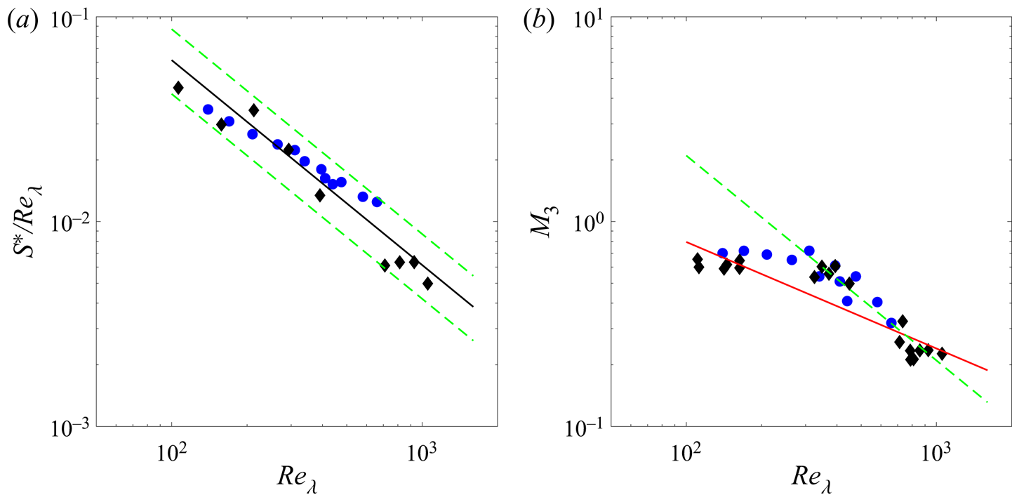
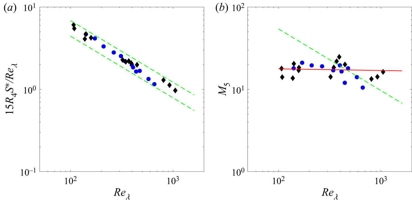
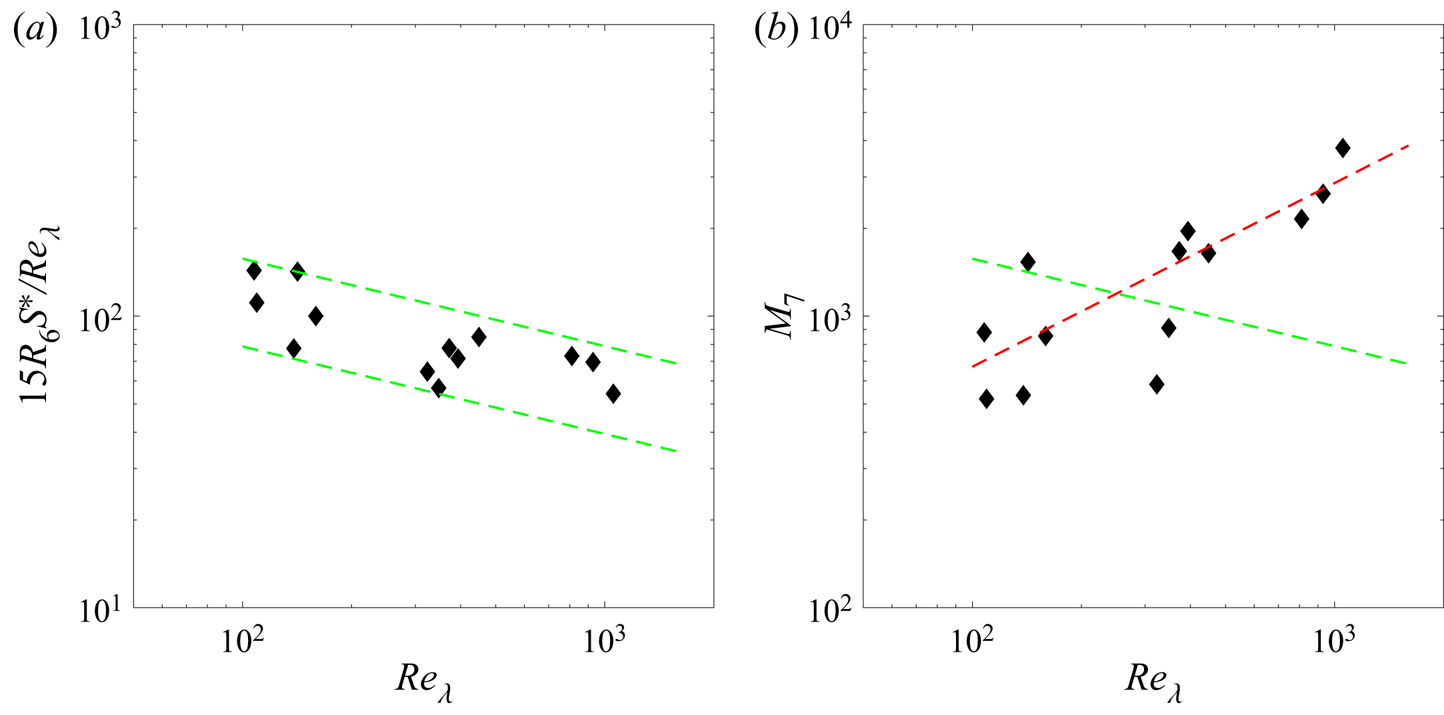
Figures 1(a), 2(a) and 3(a) show the dependence on  $Re_\lambda$ of
 $S^*/Re_\lambda$,
 $15R_4S^*/Re_\lambda$ and
 $15R_6S^*/Re_\lambda$. Due to the large scatter in these figures, we use parallel lines to encompass as much data as possible. Figures 1(b), 2(b) and 3(b) show the distributions of
 $M_3$,
 $M_5$ and
 $M_7$ versus
 $Re_\lambda$ for the same data sets. Also shown in figures 1(b), 2(b) and 3(b) are the distributions (green lines) with the same power-law exponents as in figures 1(a), 2(a) and 3(a), and the predictions of Shen & Warhaft (Reference Shen and Warhaft2000):
 $M_3= 8.72 Re_\lambda ^{-0.52}$,
 $M_5\sim Re_\lambda ^{-0.02}$ and
 $M_7\sim Re_\lambda ^{0.63}$ (red lines). The same scales for the horizontal axis and two decades for the vertical axis are used in figures 1–3. It can be seen from figure 1(a) that
 $S^*/Re_\lambda$ follows approximately the relation
 $\sim Re_\lambda ^{-1}$. Since experimental data of Shen & Warhaft (Reference Shen and Warhaft2002) show that
 $R_2=2.07$ and 1.87 at
 $Re_\lambda = 193$ and 974, respectively, we can obtain
 $S^*/Re_\lambda ={A_{1}}/15R_2\approx {A_{1}}/30$ when taking
 $R_2 \approx 2$. We can observe in figure 1(b) that
 $M_3$ follows the relation
 $\sim Re_\lambda ^{-1}$ for
 $Re_\lambda \gtrsim 200$. In contrast, the distribution for
 $8.72 Re_\lambda ^{-0.52}$ proposed by Shen & Warhaft (Reference Shen and Warhaft2000) does not follow the data well. For simplicity, the distribution for
 $S^*/Re_\lambda$ described by the black line (
 $6.14 Re_\lambda ^{-1}$) in figure 1(a) has been used to plot the distributions of
 $15R_4S^*/Re_\lambda$ and
 $15R_6S^*/Re_\lambda$ in figures 2(a) and 3(a). Figures 2(a) and 3(a) show that
 $15R_4S^*/Re_\lambda$ (
 $=A_2$) and
 $15R_6S^*/Re_\lambda$ (
 $=A_3$) decrease as
 ${\sim } Re_\lambda ^{-0.75}$ and
 ${\sim } Re_\lambda ^{-0.3}$, respectively. The results in figures 1(a), 2(a) and 3(a) indicate that both the mean shear
 $S^*$ and the even moments of transverse velocity derivatives (
 $R_2$,
 $R_4$ and
 $R_6$) affect significantly the rate at which LI is approached in the context of
 ${A_1}$,
 ${A_2}$ and
 $A_{3}$. In particular, since
 $R_2\approx 2$ (Shen & Warhaft Reference Shen and Warhaft2002),
 $R_4\sim Re_\lambda ^{0.25}$ and
 $R_6\sim Re_\lambda ^{0.7}$ (Shen & Warhaft Reference Shen and Warhaft2000), the larger the order, the slower the rate at which this approach is reached. However, despite the large scatter,
 $M_5$ is approximately constant, and
 $M_7$ increases as
 $Re_\lambda$; they do not follow the behaviour of
 ${A_2}$ and
 $A_{3}$. The reason for the difference in behaviour between
 $M_7$ and
 $A_3$,
 $M_5$ and
 $A_2$, deserves further investigation. Our analytical derivations indicate that the small-scale quantities
 ${A_1}$,
 ${A_2}$ and
 $A_{3}$ will tend towards isotropy with increasing
 $Re_\lambda$ provided that the product of the normalized even-order moments (i.e.
 $R_2$,
 $R_4$ and
 $R_6$) and
 $S^*$ does not increase as rapidly as
 $Re_\lambda$. However, other small-scale quantities, such as
 $M_7$, may not follow the same trend, or even exhibit an opposite trend. We recall that Shen & Warhaft (Reference Shen and Warhaft2000) used an active grid to achieve high
 $Re_\lambda$. The high turbulence levels generated by the active grid may potentially produce large-scale anisotropy that may induce an additional effect on the behaviour of
 $M_7$. Evidently, it would be desirable to examine the behaviour of
 $M_5$ and
 $M_7$ at higher
 $Re_\lambda$.
Dependence on  $Re_\lambda$ of (a)
 $S^*/Re_\lambda$ and (b)
 $M_3$, in the statistically stationary turbulence. Note that
 $S^*/Re_\lambda ={A_{1}}/15R_2$, see (2.16). Blue circles correspond to Ferchichi & Tavoularis (Reference Ferchichi and Tavoularis2000), and black diamonds correspond to Shen & Warhaft (Reference Shen and Warhaft2000). Green lines indicate
 ${\sim }Re_\lambda ^{-1}$, the black curve indicates
 $6.14 Re_\lambda ^{-1}$, and the red line indicates
 $8.72 Re_\lambda ^{-0.52}$ (Shen & Warhaft Reference Shen and Warhaft2000).

(a) Dependence of  $15R_4S^*/Re_\lambda$ in the statistically stationary turbulence. (b) Dependence of
 $M_5$ on
 $Re_\lambda$. Blue circles correspond to Ferchichi & Tavoularis (Reference Ferchichi and Tavoularis2000), and black diamonds correspond to Shen & Warhaft Reference Shen and Warhaft2000). Green lines indicate
 ${\sim }Re_\lambda ^{-0.75}$, and the red line indicates
 ${\sim } Re_\lambda ^{-0.02}$ (Shen & Warhaft Reference Shen and Warhaft2000).

(a) Dependence of  $15R_6S^*/Re_\lambda$ on
 $Re_\lambda$ in the statistically stationary turbulence (Shen & Warhaft Reference Shen and Warhaft2000). (b) Dependence of
 $M_7$ on
 $Re_\lambda$ (Shen & Warhaft Reference Shen and Warhaft2000). Green lines indicate
 ${\sim }Re_\lambda ^{-0.3}$, and the red line indicates
 ${\sim } Re_\lambda ^{0.63}$ (Shen & Warhaft Reference Shen and Warhaft2000).

3. Conclusions
Starting with the Navier–Stokes equations, we have derived an analytical framework to describe the relationship between the large-scale forcing caused by the mean shear and the small-scale anisotropy for statistically stationary turbulence. It is found that there is a simple relation between the mean shear and local anisotropy, i.e. (2.16). Since the available data in a stationary turbulent shear flow show that normalized second-order moments, such as  $R_2$, do not depart significantly from the isotropic value of 2, the small-scale quantity
 $A_1$ tends towards isotropy for a given non-dimensional velocity shear parameter
 ${S^*}$. This is consistent with the behaviour of
 $M_3$ for
 $Re_\lambda \gtrsim 200$ (Ferchichi & Tavoularis Reference Ferchichi and Tavoularis2000; Shen & Warhaft Reference Shen and Warhaft2000) and the conventional scaling of Lumley (Reference Lumley1967). The rate at which small scales tend towards isotropy depends on the magnitude of
 ${S^*}$ and is proportional to
 $Re_\lambda ^{-1}$. A similar analysis has been applied to the transport equations for the eighth- and twelfth-order velocity derivative moments. It is found that not only
 ${S^*}$ but also the normalized even-order moments (i.e.
 $R_4$ and
 $R_6$) will affect the rate at which small scales tend towards isotropy. The larger the product of the normalized even-order moments (
 $R_4$ and
 $R_6$) and
 ${S^*}$, the slower the rate at which small-scale quantities
 $A_2$ and
 $A_3$ tend towards isotropy as the Reynolds number increases. We should stress that the present analytical results for the behaviour of
 $A_1$,
 $A_2$ and
 $A_3$, whilst highlighting the importance of the mean shear
 $S^*$ and the normalized even-order moments (i.e.
 $R_2$,
 $R_4$ and
 $R_6$), are insufficient to allow definitive conclusions with regard to whether all the small-scale quantities in statistically stationary turbulent shear flows will tend towards isotropy.
Finally, it would be desirable to investigate further the effect of the large-scale forcing caused by the mean shear on the small-scale anisotropy by examining the corresponding transport equations for the fourth-, eighth- and twelfth-order velocity structure functions. This would allow the approach towards LI to be estimated as the scale decreases and  $Re_\lambda$ increases, and hence allow a more general assessment of the key assumption (i.e. LI) of Kolmogorov (Reference Kolmogorov1941).
Funding
S.L.T. wishes to acknowledge support given to him from NSFC through grants 11702074 and 91952109, and from the Research Grants Council of Shenzhen Government through grant RCYX20210706092046085. He also thanks his master student S.D. Chen for his very useful help to derive (B4).
Declaration of interests
The authors report no conflict of interest.
Appendix A. Large-scale production terms in (2.2)
We have examined (2.4) and (2.5) for  $i = 1$,
 $j = 2$ and
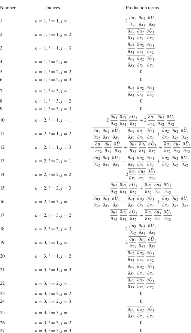
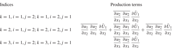
 $k = 1$. It is also desirable to examine these equations for other values of indices. Table 1 lists the large-scale production terms corresponding to all indices for the statistically stationary turbulence under a uniform mean velocity gradient in the
 $x_2$ direction. We can observe that there are only three different large-scale production terms that satisfy the condition: regardless of whether LI is satisfied, the large-scale terms are non-zero; the corresponding indices and the large-scale terms are shown in table 2. Since the term
 ${\overline { ({{\partial {u_2}}}/{{\partial {x_1}}})({{\partial {u_2}}}/{{\partial {x_1}}})}\,({{\partial {{\bar {U}}_1}}}/{{\partial {x_2}}})}$ has been discussed in detail in § 2, we now focus on only the other two production terms. As in (2.5), we normalize them and the corresponding small-scale quantities using
 $\overline {{{( {\partial {u_1}/\partial {x_1}} )}^2}}$, i.e.
 \begin{gather} \dfrac{{\overline {\dfrac{{\partial {u_2}}}{{\partial {x_3}}}\,\dfrac{{\partial {u_2}}}{{\partial {x_3}}}}\,\dfrac{{\partial {{\bar{U}}_1}}}{{\partial {x_2}}}}}{{{{\overline {{{\left( {\partial {u_1}/\partial {x_1}} \right)}^2}} }^{3/2}}}} = \dfrac{{15{R_{21}}{S^*}}}{{{Re_\lambda }}}={A_{123}}={A_{213}}, \end{gather}
 \begin{gather}\dfrac{{\overline {\dfrac{{\partial {u_1}}}{{\partial {x_2}}}\,\dfrac{{\partial {u_2}}}{{\partial {x_1}}}}\,\dfrac{{\partial {{\bar{U}}_1}}}{{\partial {x_2}}} + \overline {\dfrac{{\partial {u_2}}}{{\partial {x_2}}}\,\dfrac{{\partial {u_1}}}{{\partial {x_1}}}}\,\dfrac{{\partial {{\bar{U}}_1}}}{{\partial {x_2}}} + \overline {\dfrac{{\partial {u_2}}}{{\partial {x_2}}}\,\dfrac{{\partial {u_2}}}{{\partial {x_2}}}}\,\dfrac{{\partial {{\bar{U}}_1}}}{{\partial {x_2}}}}}{{{{\overline {{{\left( {\partial {u_1}/\partial {x_1}} \right)}^2}} }^{3/2}}}}\nonumber\\ \quad = \dfrac{{15({R_{22}} + {R_{23}} + {R_{24}}){S^*}}}{{{Re_\lambda }}}={A_{122}}={A_{212}}, \end{gather}
where  ${A_{122}}$,
 ${A_{212}}$,
 ${A_{123}}$ and
 ${A_{213}}$ are given by
 \begin{equation} {A_{ijk}} \!=\! \dfrac{{ - \overline {\dfrac{{\partial {u_i}}}{{\partial {x_k}}}\,\dfrac{{\partial {u_l}}}{{\partial {x_k}}}\,\dfrac{{\partial {u_j}}}{{\partial {x_l}}}} - \overline {\dfrac{{\partial {u_j}}}{{\partial {x_k}}}\,\dfrac{{\partial {u_l}}}{{\partial {x_k}}}\,\dfrac{{\partial {u_i}}}{{\partial {x_l}}}} - \overline {\dfrac{{\partial {u_i}}}{{\partial {x_k}}}\,\dfrac{{{\partial ^2}p}}{{\partial {x_k}\,\partial {x_j}}}} - \overline {\dfrac{{\partial {u_j}}}{{\partial {x_k}}}\,\dfrac{{{\partial ^2}p}}{{\partial {x_k}\,\partial {x_i}}}} - {\rm{2}}\nu\,\overline {\dfrac{{{\partial ^2}{u_i}}}{{\partial {x_k}\,\partial {x_l}}}\,\dfrac{{{\partial ^2}{u_j}}}{{\partial {x_k}\,\partial {x_l}}}} }}{{{{\overline {{{\left( {\partial {u_1}/\partial {x_1}} \right)}^2}} }^{3/2}}}}, \end{equation}
and the parameters  ${R_{2i}}$ (
 $i=1,2,3,4$) are defined as
 \begin{equation} \left.\begin{gathered} {R_{21}} = \frac{{\overline {{{\left( {\partial {u_2}/\partial {x_3}} \right)}^2}} }}{{\overline {{{\left( {\partial {u_1}/\partial {x_1}} \right)}^2}} }},\quad {R_{22}} = \frac{{\overline {\left( {\partial {u_1}/\partial {x_2}} \right)\left( {\partial {u_2}/\partial {x_1}} \right)} }}{{\overline {{{\left( {\partial {u_1}/\partial {x_1}} \right)}^2}} }},\\ {R_{23}} = \frac{{\overline {\left( {\partial {u_2}/\partial {x_2}} \right)\left( {\partial {u_1}/\partial {x_1}} \right)} }}{{\overline {{{\left( {\partial {u_1}/\partial {x_1}} \right)}^2}} }},\quad {R_{24}} = \frac{{\overline {{{\left( {\partial {u_2}/\partial {x_2}} \right)}^2}} }}{{\overline {{{\left( {\partial {u_1}/\partial {x_1}} \right)}^2}} }}. \end{gathered}\right\} \end{equation}
Note that  ${A_{122}}={A_{212}}={A_{123}}={A_{213}}=0$ if LI is satisfied. Like (2.5), (A1) and (A2) relate the mean shear (i.e.
 $S^*$) to a measure of local anisotropy (i.e.
 ${A_{122}}$,
 ${A_{212}}$,
 ${A_{123}}$ and
 ${A_{213}}$). Further, as discussed in the context of (2.5), LI is satisfied approximately in the context of
 $R_2$ (
 $\approx 2$) and
 $\overline {{{\left ( {\partial {u_1}/\partial {x_1}} \right )}^2}} /\overline {{{\left ( {\partial {u_1}/\partial {x_2}} \right )}^2}} \approx 0.5$ over a large range of
 $Re_\lambda$. Like these two quantities, if we assume that
 ${R_{2i}}$ (
 $i=1,2,3,4$) do not depart significantly from their isotropic values, i.e.
 $R_{21}\approx 2$,
 $R_{22}\approx -0.5$,
 $R_{23}\approx -0.5$ and
 $R_{24}\approx 1$, then (A2) indicates that
 ${A_{122}}$ and
 ${A_{212}}$ will be close to zero since
 $R_{22}+R_{23}+R_{24}\approx 0$. Further, (A1) indicates that for a given
 $S^*$, the flow will approach LI as
 $Re_\lambda ^{-1}$, similar as
 $A_1$ in (2.5).
Large-scale production terms corresponding to all indices in (2.2) for statistically stationary turbulence with a uniform mean velocity gradient in the  $x_2$ direction (i.e.
 $\partial {\bar {U}_1}/\partial {x_2} \ne 0$).

Large-scale production terms that satisfy the condition: regardless of whether LI is satisfied, the large-scale terms are non-zero. Note that since  $i\ne j$,
 ${A_{122}}$,
 ${A_{212}}$,
 ${A_{123}}$ and
 ${A_{213}}$, defined in (A3), are zero when LI is assumed.

Appendix B. Transport equations for the eighth-order velocity derivative moments
The dynamic equation for the velocity fluctuation  $u_j$ is given by (e.g. Pope Reference Pope2000)
 \begin{equation} \frac{{\partial {u_j}}}{{\partial t}} + {\bar{U} _l}\,\frac{{\partial {u_j}}}{{\partial {x_l}}} + {u_l}\,\frac{{\partial {u_j}}}{{\partial {x_l}}} + {u_l}\,\frac{{\partial {{\bar{U} }_j}}}{{\partial {x_l}}} - \frac{{\partial \overline {{u_j}{u_l}} }}{{\partial {x_l}}} + \frac{{\partial p}}{{\partial {x_j}}} - \nu\,\frac{\partial }{{\partial {x_l}}}\frac{{\partial {u_j}}}{{\partial {x_l}}} = 0. \end{equation}
We first differentiate (B1) with respect to  $x_k$ (
 $k=1,2,3$), and then multiply by
 ${{(\partial {u_i}}/{\partial {x_k})}}({{\partial {u_m}}/ {\partial {x_k}}})({{\partial {u_n}} / {\partial {x_k}}})$ to obtain
 \begin{align} &\frac{{\partial {u_i}}}{{\partial {x_k}}}\,\frac{{\partial {u_m}}}{{\partial {x_k}}}\,\frac{{\partial {u_n}}}{{\partial {x_k}}}\,\frac{\partial }{{\partial {x_k}}}\left( {\frac{{\partial {u_j}}}{{\partial t}}} \right) + \frac{{\partial {u_i}}}{{\partial {x_k}}}\,\frac{{\partial {u_m}}}{{\partial {x_k}}}\,\frac{{\partial {u_n}}}{{\partial {x_k}}}\,\frac{\partial }{{\partial {x_k}}}\left( {{{\bar{U} }_l}\,\frac{{\partial {u_j}}}{{\partial {x_l}}}} \right) \nonumber\\ &\quad +\frac{{\partial {u_i}}}{{\partial {x_k}}}\,\frac{{\partial {u_m}}}{{\partial {x_k}}}\,\frac{{\partial {u_n}}}{{\partial {x_k}}}\,\frac{\partial }{{\partial {x_k}}}\left( {{u_l}\,\frac{{\partial {u_j}}}{{\partial {x_l}}}} \right)+ \frac{{\partial {u_i}}}{{\partial {x_k}}}\,\frac{{\partial {u_m}}}{{\partial {x_k}}}\,\frac{{\partial {u_n}}}{{\partial {x_k}}}\,\frac{\partial }{{\partial {x_k}}}\left( {{u_l}\,\frac{{\partial {{\bar{U} }_j}}}{{\partial {x_l}}}} \right) \nonumber\\ &\quad-\frac{{\partial {u_i}}}{{\partial {x_k}}}\,\frac{{\partial {u_m}}}{{\partial {x_k}}}\,\frac{{\partial {u_n}}}{{\partial {x_k}}}\,\frac{\partial }{{\partial {x_k}}}\left( {\frac{{\partial \overline {{u_j}{u_l}} }}{{\partial {x_l}}}} \right) + \frac{{\partial {u_i}}}{{\partial {x_k}}}\,\frac{{\partial {u_m}}}{{\partial {x_k}}}\,\frac{{\partial {u_n}}}{{\partial {x_k}}}\,\frac{\partial }{{\partial {x_k}}}\left( {\frac{{\partial p}}{{\partial {x_j}}}} \right) \nonumber\\ &\quad -\nu\,\frac{{\partial {u_i}}}{{\partial {x_k}}}\,\frac{{\partial {u_m}}}{{\partial {x_k}}}\,\frac{{\partial {u_n}}}{{\partial {x_k}}}\,\frac{\partial }{{\partial {x_k}}}\left( {\frac{{{\partial ^2}{u_j}}}{{\partial x_l^2}}} \right) = 0. \end{align}
We now add (B2) to itself with  $i$ and
 $j$ transposed, with
 $m$ and
 $j$ transposed, also with
 $n$ and
 $j$ transposed, and then apply averaging to obtain

Using the same assumptions as associated with (2.2), i.e. the flow is statistically stationary turbulence under a uniform mean velocity gradient in the  $x_2$ direction, the above equation reduces to
 \begin{align} &\overline {\frac{{\partial {u_i}}}{{\partial {x_k}}}\,\frac{{\partial {u_m}}}{{\partial {x_k}}}\,\frac{{\partial {u_n}}}{{\partial {x_k}}}\,\frac{{\partial {u_j}}}{{\partial {x_l}}}}\,\frac{{\partial {{\bar{U} }_l}}}{{\partial {x_k}}} + \overline {\frac{{\partial {u_j}}}{{\partial {x_k}}}\,\frac{{\partial {u_m}}}{{\partial {x_k}}}\,\frac{{\partial {u_n}}}{{\partial {x_k}}}\,\frac{{\partial {u_i}}}{{\partial {x_l}}}}\,\frac{{\partial {{\bar{U} }_l}}}{{\partial {x_k}}}\nonumber\\ &\qquad + \overline {\frac{{\partial {u_i}}}{{\partial {x_k}}}\,\frac{{\partial {u_j}}}{{\partial {x_k}}}\,\frac{{\partial {u_n}}}{{\partial {x_k}}}\,\frac{{\partial {u_m}}}{{\partial {x_l}}}}\, \frac{{\partial {{\bar{U} }_l}}}{{\partial {x_k}}} + \overline {\frac{{\partial {u_i}}}{{\partial {x_k}}}\,\frac{{\partial {u_m}}}{{\partial {x_k}}}\,\frac{{\partial {u_j}}}{{\partial {x_k}}}\,\frac{{\partial {u_n}}}{{\partial {x_l}}}}\,\frac{{\partial {{\bar{U} }_l}}}{{\partial {x_k}}} + \overline {\frac{{\partial {u_i}}}{{\partial {x_k}}}\,\frac{{\partial {u_m}}}{{\partial {x_k}}}\,\frac{{\partial {u_n}}}{{\partial {x_k}}}\,\frac{{\partial {u_l}}}{{\partial {x_k}}}}\,\frac{{\partial {{\bar{U} }_j}}}{{\partial {x_l}}}\nonumber\\ &\qquad + \overline {\frac{{\partial {u_j}}}{{\partial {x_k}}}\,\frac{{\partial {u_m}}}{{\partial {x_k}}}\,\frac{{\partial {u_n}}}{{\partial {x_k}}}\,\frac{{\partial {u_l}}}{{\partial {x_k}}}}\, \frac{{\partial {{\bar{U} }_i}}}{{\partial {x_l}}} + \overline {\frac{{\partial {u_i}}}{{\partial {x_k}}}\,\frac{{\partial {u_j}}}{{\partial {x_k}}}\,\frac{{\partial {u_n}}}{{\partial {x_k}}}\,\frac{{\partial {u_l}}}{{\partial {x_k}}}}\,\frac{{\partial {{\bar{U} }_m}}}{{\partial {x_l}}} + \overline {\frac{{\partial {u_i}}}{{\partial {x_k}}}\,\frac{{\partial {u_m}}}{{\partial {x_k}}}\,\frac{{\partial {u_j}}}{{\partial {x_k}}}\,\frac{{\partial {u_l}}}{{\partial {x_k}}}}\,\frac{{\partial {{\bar{U} }_n}}}{{\partial {x_l}}}\nonumber\\ &\quad ={-} \overline {\frac{{\partial {u_i}}}{{\partial {x_k}}}\,\frac{{\partial {u_m}}}{{\partial {x_k}}}\,\frac{{\partial {u_n}}}{{\partial {x_k}}}\,\frac{{\partial {u_l}}}{{\partial {x_k}}}\,\frac{{\partial {u_j}}}{{\partial {x_l}}}} - \overline {\frac{{\partial {u_j}}}{{\partial {x_k}}}\,\frac{{\partial {u_m}}}{{\partial {x_k}}}\,\frac{{\partial {u_n}}}{{\partial {x_k}}}\,\frac{{\partial {u_l}}}{{\partial {x_k}}}\,\frac{{\partial {u_i}}}{{\partial {x_l}}}}\nonumber\\ &\qquad - \overline {\frac{{\partial {u_i}}}{{\partial {x_k}}}\,\frac{{\partial {u_j}}}{{\partial {x_k}}}\,\frac{{\partial {u_n}}}{{\partial {x_k}}}\,\frac{{\partial {u_l}}}{{\partial {x_k}}}\,\frac{{\partial {u_m}}}{{\partial {x_l}}}} - \overline {\frac{{\partial {u_i}}}{{\partial {x_k}}}\,\frac{{\partial {u_m}}}{{\partial {x_k}}}\,\frac{{\partial {u_j}}}{{\partial {x_k}}}\,\frac{{\partial {u_l}}}{{\partial {x_k}}}\,\frac{{\partial {u_n}}}{{\partial {x_l}}}} \nonumber\\ &\qquad - \overline {\frac{{\partial {u_i}}}{{\partial {x_k}}}\,\frac{{\partial {u_m}}}{{\partial {x_k}}}\,\frac{{\partial {u_n}}}{{\partial {x_k}}}\,\frac{\partial }{{\partial {x_k}}}\left( {\frac{{\partial p}}{{\partial {x_j}}}} \right)} - \overline {\frac{{\partial {u_j}}}{{\partial {x_k}}}\,\frac{{\partial {u_m}}}{{\partial {x_k}}}\,\frac{{\partial {u_n}}}{{\partial {x_k}}}\,\frac{\partial }{{\partial {x_k}}}\left( {\frac{{\partial p}}{{\partial {x_i}}}} \right)}\nonumber\\ &\qquad - \overline {\frac{{\partial {u_i}}}{{\partial {x_k}}}\,\frac{{\partial {u_j}}}{{\partial {x_k}}}\,\frac{{\partial {u_n}}}{{\partial {x_k}}}\,\frac{\partial }{{\partial {x_k}}}\left( {\frac{{\partial p}}{{\partial {x_m}}}} \right)} - \overline {\frac{{\partial {u_i}}}{{\partial {x_k}}}\,\frac{{\partial {u_m}}}{{\partial {x_k}}}\,\frac{{\partial {u_j}}}{{\partial {x_k}}}\,\frac{\partial }{{\partial {x_k}}}\left( {\frac{{\partial p}}{{\partial {x_n}}}} \right)}\nonumber\\ &\qquad - \nu\,\overline {\frac{{{\partial ^2}{u_j}}}{{\partial {x_k}\,\partial {x_l}}}\,\frac{\partial }{{\partial {x_l}}}\left( {\frac{{\partial {u_i}}}{{\partial {x_k}}}\,\frac{{\partial {u_m}}}{{\partial {x_k}}}\,\frac{{\partial {u_n}}}{{\partial {x_k}}}} \right)} - \nu\,\overline {\frac{{{\partial ^2}{u_i}}}{{\partial {x_k}\,\partial {x_l}}}\,\frac{\partial }{{\partial {x_l}}}\left( {\frac{{\partial {u_j}}}{{\partial {x_k}}}\,\frac{{\partial {u_m}}}{{\partial {x_k}}}\,\frac{{\partial {u_n}}}{{\partial {x_k}}}} \right)} \nonumber\\ &\qquad - \nu\,\overline {\frac{{{\partial ^2}{u_m}}}{{\partial {x_k}\,\partial {x_l}}}\,\frac{\partial }{{\partial {x_l}}}\left( {\frac{{\partial {u_i}}}{{\partial {x_k}}}\,\frac{{\partial {u_j}}}{{\partial {x_k}}}\,\frac{{\partial {u_n}}}{{\partial {x_k}}}} \right)} - \nu\,\overline {\frac{{{\partial ^2}{u_n}}}{{\partial {x_k}\,\partial {x_l}}}\frac{\partial }{{\partial {x_l}}}\left( {\frac{{\partial {u_i}}}{{\partial {x_k}}}\,\frac{{\partial {u_m}}}{{\partial {x_k}}}\,\frac{{\partial {u_j}}}{{\partial {x_k}}}} \right)}. \end{align}
The eight terms on the first, second and third lines are the large-scale production terms associated with the mean shear, which will be simplified after taking the values for  $i$,
 $j$,
 $k$,
 $m$ and
 $n$ (see below). The other terms are small-scale terms. Since
 $i$,
 $j$,
 $k$,
 $m$ and
 $n$ can assume values of 1, 2 and 3, there are 243 independent equations in (B4). Like (2.5), we take
 $k=n=1$ and
 $i=j=m = 2$, and (B4) becomes
 \begin{align} \overline {{{\left( {\frac{{\partial {u_2}}}{{\partial {x_1}}}} \right)}^4}} \frac{{\partial {{\bar{U} }_1}}}{{\partial {x_2}}} &={-} 3\,\overline {{{\left( {\frac{{\partial {u_2}}}{{\partial {x_1}}}} \right)}^2}\frac{{\partial {u_1}}}{{\partial {x_1}}}\,\frac{{\partial {u_l}}}{{\partial {x_1}}}\,\frac{{\partial {u_2}}}{{\partial {x_l}}}} - \overline {{{\left( {\frac{{\partial {u_2}}}{{\partial {x_1}}}} \right)}^3}\frac{{\partial {u_l}}}{{\partial {x_1}}}\,\frac{{\partial {u_1}}}{{\partial {x_l}}}}\nonumber\\ &\quad - 3\,\overline {{{\left( {\frac{{\partial {u_2}}}{{\partial {x_1}}}} \right)}^2}\frac{{\partial {u_1}}}{{\partial {x_1}}}\,\frac{\partial }{{\partial {x_1}}}\left( {\frac{{\partial p}}{{\partial {x_2}}}} \right)} - \overline {{{\left( {\frac{{\partial {u_2}}}{{\partial {x_1}}}} \right)}^3}\frac{\partial }{{\partial {x_1}}}\left( {\frac{{\partial p}}{{\partial {x_1}}}} \right)}\nonumber\\ &\quad - 3\nu\,\overline {\frac{{{\partial ^2}{u_2}}}{{\partial {x_1}\,\partial {x_l}}}\,\frac{\partial }{{\partial {x_l}}}\left( {{{\left( {\frac{{\partial {u_2}}}{{\partial {x_1}}}} \right)}^2}\frac{{\partial {u_1}}}{{\partial {x_1}}}} \right)} - \nu\,\overline {\frac{{{\partial ^2}{u_1}}}{{\partial {x_1}\,\partial {x_l}}}\,\frac{\partial }{{\partial {x_l}}}{{\left( {\frac{{\partial {u_2}}}{{\partial {x_1}}}} \right)}^3}}, \end{align}
which, after normalizing by  $\overline {{{\left ( {\partial {u_1}/\partial {x_1}} \right )}^2}}$, becomes
 \begin{align} \frac{{\overline {{{\left( {\dfrac{{\partial {u_2}}}{{\partial {x_1}}}} \right)}^4}} \dfrac{{\partial {{\bar{U}}_1}}}{{\partial {x_2}}}}}{{{{\overline {{{\left( {\partial {u_1}/\partial {x_1}} \right)}^2}} }^{5/2}}}} &= \frac{{\overline {{{\left( {\dfrac{{\partial {u_2}}}{{\partial {x_1}}}} \right)}^4}} \dfrac{{\partial {{\bar{U}}_1}}}{{\partial {x_2}}}}}{{{{\overline {{{\left( {\partial {u_1}/\partial {x_1}} \right)}^2}} }^2}\,{{\overline {{{\left( {\partial {u_1}/\partial {x_1}} \right)}^2}} }^{1/2}}}} \nonumber\\ &= {R_4}\,\frac{{\partial {{\bar{U}}_1}/\partial {x_2}}}{{{{\overline {{{\left( {\partial {u_1}/\partial {x_1}} \right)}^2}} }^{1/2}}}} = {R_4}\,\frac{{15\nu\,\overline {{u^2}}\,\partial {{\bar{U}}_1}/\partial {x_2}\,{{\overline {{{\left( {\partial {u_1}/\partial {x_1}} \right)}^2}} }^{1/2}}}}{{15\nu\,\overline {{u^2}}\,\overline {{{\left( {\partial {u_1}/\partial {x_1}} \right)}^2}} }}\nonumber\\ &= {R_4}\,\frac{{15\nu\,\overline {{u^2}}\,\partial {{\bar{U}}_1}/\partial {x_2}\,{{\overline {{{\left( {\partial {u_1}/\partial {x_1}} \right)}^2}} }^{1/2}}}}{{\overline {{u^2}}\,{{\overline \varepsilon }_{iso}}}} = {R_4}\,\frac{{{S^*}15\nu\,{{\overline {{{\left( {\partial {u_1}/\partial {x_1}} \right)}^2}} }^{1/2}}}}{{\overline {{u^2}} }}\nonumber\\ &= \frac{{15{R_4}{S^*}}}{{Re_\lambda }} = {A_2}, \end{align}
where  $R_4$ and
 ${A_2}$ are defined in (2.11) and (2.12), respectively.
Appendix C. Transport equations for the twelfth- order velocity derivative moments
As in Appendix B, we first differentiate (B1) with respect to  $x_k$ (
 $k=1,2,3$), and then multiply by
 ${{(\partial {u_i}}/{\partial {x_k})}}({{\partial {u_m}}/ {\partial {x_k}}})({{\partial {u_n}} / {\partial {x_k}}})({{\partial {u_{t}}} / {\partial {x_k}}})({{\partial {u_q}} / {\partial {x_k}}})$ to obtain
 \begin{align} &\frac{{\partial {u_i}}}{{\partial {x_k}}}\,\frac{{\partial {u_m}}}{{\partial {x_k}}}\,\frac{{\partial {u_n}}}{{\partial {x_k}}}\,\frac{{\partial {u_{t}}}}{{\partial {x_k}}}\,\frac{{\partial {u_q}}}{{\partial {x_k}}}\,\frac{\partial }{{\partial {x_k}}}\left( {\frac{{\partial {u_j}}}{{\partial t}}} \right) + \frac{{\partial {u_i}}}{{\partial {x_k}}}\,\frac{{\partial {u_m}}}{{\partial {x_k}}}\,\frac{{\partial {u_n}}}{{\partial {x_k}}}\,\frac{{\partial {u_{t}}}}{{\partial {x_k}}}\,\frac{{\partial {u_q}}}{{\partial {x_k}}}\,\frac{\partial }{{\partial {x_k}}}\left( {{{\bar{U} }_l}\frac{{\partial {u_j}}}{{\partial {x_l}}}} \right)\nonumber\\ &\quad + \frac{{\partial {u_i}}}{{\partial {x_k}}}\,\frac{{\partial {u_m}}}{{\partial {x_k}}}\,\frac{{\partial {u_n}}}{{\partial {x_k}}}\,\frac{{\partial {u_{t}}}}{{\partial {x_k}}}\,\frac{{\partial {u_q}}}{{\partial {x_k}}}\,\frac{\partial }{{\partial {x_k}}}\left( {{u_l}\frac{{\partial {u_j}}}{{\partial {x_l}}}} \right) + \frac{{\partial {u_i}}}{{\partial {x_k}}}\,\frac{{\partial {u_m}}}{{\partial {x_k}}}\,\frac{{\partial {u_n}}}{{\partial {x_k}}}\,\frac{{\partial {u_{t}}}}{{\partial {x_k}}}\,\frac{{\partial {u_q}}}{{\partial {x_k}}}\,\frac{\partial }{{\partial {x_k}}}\left( {{u_l}\frac{{\partial {{\bar{U} }_j}}}{{\partial {x_l}}}} \right)\nonumber\\ &\quad - \frac{{\partial {u_i}}}{{\partial {x_k}}}\,\frac{{\partial {u_m}}}{{\partial {x_k}}}\,\frac{{\partial {u_n}}}{{\partial {x_k}}}\,\frac{{\partial {u_{t}}}}{{\partial {x_k}}}\,\frac{{\partial {u_q}}}{{\partial {x_k}}}\,\frac{\partial }{{\partial {x_k}}}\left( {\frac{{\partial \overline {{u_j}{u_l}} }}{{\partial {x_l}}}} \right) + \frac{{\partial {u_i}}}{{\partial {x_k}}}\,\frac{{\partial {u_m}}}{{\partial {x_k}}}\,\frac{{\partial {u_n}}}{{\partial {x_k}}}\,\frac{{\partial {u_{t}}}}{{\partial {x_k}}}\,\frac{{\partial {u_q}}}{{\partial {x_k}}}\,\frac{\partial }{{\partial {x_k}}}\left( {\frac{{\partial p}}{{\partial {x_j}}}} \right)\nonumber\\ &\quad - \nu\,\frac{{\partial {u_i}}}{{\partial {x_k}}}\,\frac{{\partial {u_m}}}{{\partial {x_k}}}\,\frac{{\partial {u_n}}}{{\partial {x_k}}}\,\frac{{\partial {u_{t}}}}{{\partial {x_k}}}\,\frac{{\partial {u_q}}}{{\partial {x_k}}}\,\frac{\partial }{{\partial {x_k}}}\left( {\frac{{{\partial ^2}{u_j}}}{{\partial x_l^2}}} \right) = 0. \end{align}
We now add (C1) to itself with  $i$ and
 $j$ transposed, with
 $m$ and
 $j$ transposed, with
 $n$ and
 $j$ transposed, with
 $p$ and
 $j$ transposed, and also with
 $q$ and
 $j$ transposed, and then average to obtain

Using the same assumptions associated with (2.2), i.e. the flow is statistically stationary turbulence under a uniform mean velocity gradient in the  $x_2$ direction, and then taking
 $k=n=1$ and
 $i=j=m=p=q = 2$, the above equation becomes
 \begin{align} \overline {{{\left( {\frac{{\partial {u_2}}}{{\partial {x_1}}}} \right)}^6}} \frac{{\partial {{\bar{U} }_1}}}{{\partial {x_2}}} &={-} 5\,\overline {{{\left( {\frac{{\partial {u_2}}}{{\partial {x_1}}}} \right)}^4}\frac{{\partial {u_1}}}{{\partial {x_1}}}\,\frac{{\partial {u_l}}}{{\partial {x_1}}}\,\frac{{\partial {u_2}}}{{\partial {x_l}}}} - \overline {{{\left( {\frac{{\partial {u_2}}}{{\partial {x_1}}}} \right)}^4}\frac{{\partial {u_2}}}{{\partial {x_1}}}\,\frac{{\partial {u_l}}}{{\partial {x_1}}}\,\frac{{\partial {u_1}}}{{\partial {x_l}}}} \nonumber\\ &\quad - 5\,\overline {{{\left( {\frac{{\partial {u_2}}}{{\partial {x_1}}}} \right)}^4}\frac{{\partial {u_1}}}{{\partial {x_1}}}\,\frac{\partial }{{\partial {x_1}}}\left( {\frac{{\partial p}}{{\partial {x_2}}}} \right)} - \overline {{{\left( {\frac{{\partial {u_2}}}{{\partial {x_1}}}} \right)}^5}\frac{\partial }{{\partial {x_1}}}\left( {\frac{{\partial p}}{{\partial {x_1}}}} \right)}\nonumber\\ &\quad- 5\nu\,\overline {\frac{{{\partial ^2}{u_2}}}{{\partial {x_1}\,\partial {x_l}}}\,\frac{\partial }{{\partial {x_l}}}\left( {{{\left( {\frac{{\partial {u_2}}}{{\partial {x_1}}}} \right)}^4}\frac{{\partial {u_1}}}{{\partial {x_1}}}} \right)} - \nu\,\overline {\frac{{{\partial ^2}{u_1}}}{{\partial {x_1}\,\partial {x_l}}}\,\frac{\partial }{{\partial {x_l}}}{{\left( {\frac{{\partial {u_2}}}{{\partial {x_1}}}} \right)}^5}}, \end{align}
which, after normalizing by  $\overline {{{\left ( {\partial {u_1}/\partial {x_1}} \right )}^2}}$, becomes
 \begin{align} \frac{{\overline {{{\left( {\dfrac{{\partial {u_2}}}{{\partial {x_1}}}} \right)}^6}} \dfrac{{\partial {{\bar{U}}_1}}}{{\partial {x_2}}}}}{{{{\overline {{{\left( {\partial {u_1}/\partial {x_1}} \right)}^2}} }^{7/2}}}} &= \dfrac{{\overline {{{\left( {\dfrac{{\partial {u_2}}}{{\partial {x_1}}}} \right)}^6}} \dfrac{{\partial {{\bar{U}}_1}}}{{\partial {x_2}}}}}{{{{\overline {{{\left( {\partial {u_1}/\partial {x_1}} \right)}^2}} }^3}\,{{\overline {{{\left( {\partial {u_1}/\partial {x_1}} \right)}^2}} }^{1/2}}}} \nonumber\\ &= {R_6}\,\frac{{\partial {{\bar{U}}_1}/\partial {x_2}}}{{{{\overline {{{\left( {\partial {u_1}/\partial {x_1}} \right)}^2}} }^{1/2}}}} = {R_6}\,\frac{{15\nu\,\overline {{u^2}}\,\partial {{\bar{U}}_1}/\partial {x_2}\,{{\overline {{{\left( {\partial {u_1}/\partial {x_1}} \right)}^2}} }^{1/2}}}}{{15\nu\,\overline {{u^2}}\,\overline {{{\left( {\partial {u_1}/\partial {x_1}} \right)}^2}} }}\nonumber\\ &= {R_6}\,\frac{{15\nu\,\overline {{u^2}}\,\partial {{\bar{U}}_1}/\partial {x_2}\,{{\overline {{{\left( {\partial {u_1}/\partial {x_1}} \right)}^2}} }^{1/2}}}}{{\overline {{u^2}}\,{{\overline \varepsilon }_{iso}}}} = {R_6}\,\frac{{{S^*}15\nu\,{{\overline {{{\left( {\partial {u_1}/\partial {x_1}} \right)}^2}} }^{1/2}}}}{{\overline {{u^2}} }} \nonumber\\ &= \frac{{15{R_6}{S^*}}}{{Re_\lambda }} = {A_3}, \end{align}
where  $R_6$ and
 ${A_3}$ are defined in (2.13) and (2.14), respectively. Note that in (B6) and (C4), the behaviours of
 $R_4$,
 $R_6$ and
 $S^*$ are already available for this flow (Shen & Warhaft Reference Shen and Warhaft2000; Schumacher et al. Reference Schumacher, Sreenivasan and Yeung2003), thus the behaviours of
 ${A_2}$ and
 ${A_3}$ can be estimated.