

1 Introduction
Swimming cells such as algae, bacteria or sperms often navigate through environments having inhomogeneous viscosity (Berg Reference Berg2004; Fauci & Dillon Reference Fauci and Dillon2006). For example, biological fluids such as mucus or extracellular polymeric substances produced by microbes are mixtures of fluids having different viscosities. Even organisms living in aquatic environments such as oceans or lakes are subjected to viscosity gradients due to the non-uniform ambient temperature or salinity (Arrigo et al. Reference Arrigo, Robinson, Worthen, Dunbar, DiTullio, VanWoert and Lizotte1999). In this paper, we focus on understanding the motion of swimmers in environments with spatial viscosity gradients.
Understanding the motion of swimmers in environments having inhomogeneous properties has been a subject of continuing investigation. For example, there are studies on the motion of swimmers in fluids having spatially varying ambient density (Ardekani & Stocker Reference Ardekani and Stocker2010; Doostmohammadi, Stocker & Ardekani Reference Doostmohammadi, Stocker and Ardekani2012; Dandekar, Shaik & Ardekani Reference Dandekar, Shaik and Ardekani2019), in heterogeneous gels (Leshansky Reference Leshansky2009; Nganguia & Pak Reference Nganguia and Pak2018) and in two-phase viscous fluids (Du et al. Reference Du, Keener, Guy and Fogelson2012). Relatively few studies have focused on the motion of swimmers in fluids having inhomogeneous viscosity. It has been observed that some micro-organisms have the ability to adapt their motion in response to external viscosity gradients, known as viscotaxis. For example, micro-organisms like Spiroplasma and Leptospira interrogans migrate towards regions of higher viscosities (positive viscotaxis) (Petrino & Doetsch Reference Petrino and Doetsch1978; Daniels, Longland & Gilbart Reference Daniels, Longland and Gilbart1980; Takabe et al. Reference Takabe, Tahara, Islam, Affroze, Kudo and Nakamura2017), while Escherichia coli migrates towards regions of lower viscosities (negative viscotaxis) (Sherman, Timkina & Glagolev Reference Sherman, Timkina and Glagolev1982). Although the physical reason for such behaviour is not well understood, Liebchen et al. (Reference Liebchen, Monderkamp, ten Hagen and Löwen2018) recently suggested that the viscous torque experienced by the swimmer due to its asymmetric shape could be the cause of the preferential alignment. Stehnach (Reference Stehnach2019) showed that swimming biflagellates (wild-type Chlamydomonas reinhardtii) have a tendency to accumulate in high-viscosity regions due to the local reduction in the swimming speed.
There are limited theoretical works that have explored the influence of viscosity gradients on the propulsion of swimmers. Shoele & Eastham (Reference Shoele and Eastham2018) studied the motion of spherical squirmers in a fluid with viscosity gradients generated due to a spatially varying nutrient concentration field. They reported the effect of the Péclet number on the squirmer swimming speed and the nutrient distribution around the squirmer. Datt & Elfring (Reference Datt and Elfring2019) studied the motion of squirmers in a fluid having a non-uniform viscosity. By assuming a linear viscosity profile, they found that axisymmetric squirmers turn towards regions of lower viscosities. From the current state of the literature, we understand that additional theoretical works are needed to shed more light on the influence of viscosity gradients on swimmers. In particular, to the best of our knowledge, there are no theoretical studies to understand the motion of swimmers such as a mammalian spermatozoon that have a single long flagella and propel by passing transverse waves along their surface. Such swimmers can be more accurately represented by a swimming sheet model (Lauga & Powers Reference Lauga and Powers2009). Studies have shown that sperms exhibit significantly different wave forms in fluids having different viscosities (Kirkman-Brown & Smith Reference Kirkman-Brown and Smith2011). Hence, to accurately represent the sperm dynamics in a viscosity-stratified medium, the compliance of the sheet should be considered. Such a coupled fluid–body interaction is difficult to solve analytically, and computational methods have to be used, which is beyond the scope of the current work.
We have studied the motion of a swimming sheet in a density-stratified fluid previously (Dandekar et al. Reference Dandekar, Shaik and Ardekani2019). However, analysing the combined influence of viscosity and density stratification is not straightforward due to the nonlinear governing equations of motion. This analysis forms an interesting future work, which is beyond the scope of the present work. Hence, we only consider viscosity stratification and assume the density dependence on the distribution of the stratifying agent to be negligible as compared to the ambient density. It is shown that, for some common examples in nature where both the density and viscosity of the fluid change due to temperature or variation in the salt concentration, the extent of the viscosity variation with the stratifying agent is much larger as compared to the density variation (Boufadel, Suidan & Venosa Reference Boufadel, Suidan and Venosa1999; Jacquemin et al. Reference Jacquemin, Husson, Padua and Majer2006). For example, it was shown that, for a unit change in temperature, the density changes for some ionic liquids were less than  $0.1\,\%$ of the ambient density, while the viscosity changes were of the order of magnitude of the ambient viscosity (Jacquemin et al. Reference Jacquemin, Husson, Padua and Majer2006). For stratification induced due to the transport of salt in water, the linear dependence of the water viscosity and density with salt concentration was obtained by fitting a regression curve to the data (Boufadel et al. Reference Boufadel, Suidan and Venosa1999). It is found that the coefficient that relates the non-dimensional viscosity and density to the salt concentration in water is more than an order of magnitude higher for viscosity as compared to density (
 $1.566\times 10^{-3}$ for viscosity and
 $6.46\times 10^{-4}$ for density). Even in the case of macromolecular solutions, such as proteins, the influence of the protein concentration on the solution viscosity is considered to be much more important than the solution density. For example, for some globular proteins such as lysozyme, the solution viscosity is observed to be much more sensitive to the protein concentration than the solution density (Fredericks et al. Reference Fredericks, Hammonds, Howard and Rosenberger1994). We, thus, assume the fluid density to be constant in our analysis.
In this work, we derive an expression for the swimming velocity in a viscosity-stratified fluid. We model the swimmer as a two-dimensional infinitely long sheet that propels by sending waves of small amplitude along its surface. Several micro-organisms such as human spermatozoon (Taylor Reference Taylor1951), flat ciliated Paramecium, Opalina (Blake Reference Blake1971) and Caenorhabditis elegans (Sznitman et al. Reference Sznitman, Purohit, Krajacic, Lamitina and Arratia2010) can be represented using this model. We analyse the effect of the viscosity stratification on the propulsion of the swimmer in the low-Reynolds-number regime. We make predictions about the effect of viscosity gradients on the motility characteristics, such as the power expenditure and the swimming efficiency.
2 Problem formulation
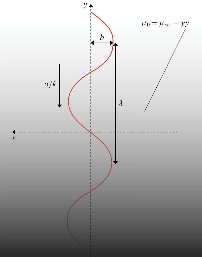
Figure 1 shows a neutrally buoyant swimming sheet immersed in a viscosity-stratified fluid of density  $\unicode[STIX]{x1D70C}_{\infty }$. We assume that the viscosity of the ambient fluid changes linearly with the vertical coordinate and is given by
 $$\begin{eqnarray}\unicode[STIX]{x1D707}_{0}=\unicode[STIX]{x1D707}_{\infty }-\unicode[STIX]{x1D6FE}y.\end{eqnarray}$$
Here,  $\unicode[STIX]{x1D707}_{\infty }$ is the reference fluid viscosity and
 $\unicode[STIX]{x1D6FE}$ is the viscosity gradient. The swimmer propels by passing a transverse wave of amplitude
 $b$, wavelength
 $2\unicode[STIX]{x03C0}/k$ and speed
 $\unicode[STIX]{x1D70E}/k$ along its surface. Hence, the surface deformation of the swimmer is given by
 $x=b\sin (ky+\unicode[STIX]{x1D70E}t)$. We further assume that the wave amplitude is much smaller than the wavelength (
 $bk\ll 1$).
Swimming sheet immersed in a viscosity-stratified fluid with ambient viscosity  $\unicode[STIX]{x1D707}_{0}=\unicode[STIX]{x1D707}_{\infty }-\unicode[STIX]{x1D6FE}y$, where gravity
 $\boldsymbol{g}$ points in the negative
 $y$ direction.

2.1 Governing equations
Owing to the small scales relevant to the swimming of micro-organisms, the Reynolds number is small and the inertia of the fluid is not important. We thus neglect inertia in our analysis. We now begin by writing the mass conservation and the momentum conservation equations in the fluid as follows:
 $$\begin{eqnarray}\displaystyle & \displaystyle \frac{\unicode[STIX]{x2202}u}{\unicode[STIX]{x2202}x}+\frac{\unicode[STIX]{x2202}v}{\unicode[STIX]{x2202}y}=0, & \displaystyle\end{eqnarray}$$
 $$\begin{eqnarray}\displaystyle & \displaystyle 0=-\frac{\unicode[STIX]{x2202}p}{\unicode[STIX]{x2202}x}+\frac{\unicode[STIX]{x2202}}{\unicode[STIX]{x2202}x}\left(\unicode[STIX]{x1D707}\frac{\unicode[STIX]{x2202}u}{\unicode[STIX]{x2202}x}\right)+\frac{\unicode[STIX]{x2202}}{\unicode[STIX]{x2202}y}\left(\unicode[STIX]{x1D707}\frac{\unicode[STIX]{x2202}u}{\unicode[STIX]{x2202}y}\right), & \displaystyle\end{eqnarray}$$
 $$\begin{eqnarray}\displaystyle & \displaystyle 0=-\frac{\unicode[STIX]{x2202}p}{\unicode[STIX]{x2202}y}-\unicode[STIX]{x1D70C}_{\infty }g+\frac{\unicode[STIX]{x2202}}{\unicode[STIX]{x2202}x}\left(\unicode[STIX]{x1D707}\frac{\unicode[STIX]{x2202}v}{\unicode[STIX]{x2202}x}\right)+\frac{\unicode[STIX]{x2202}}{\unicode[STIX]{x2202}y}\left(\unicode[STIX]{x1D707}\frac{\unicode[STIX]{x2202}v}{\unicode[STIX]{x2202}y}\right). & \displaystyle\end{eqnarray}$$
Here,  $u$ and
 $v$ represent the velocity fields in the
 $x$ and
 $y$ directions, respectively. The equations are written in the frame of reference of the swimming sheet, which is translating with a constant velocity
 $V$ in the positive
 $y$ direction.
In addition, we have the advection–diffusion equation describing the distribution of the stratifying agent. For a linear variation of viscosity with the temperature/concentration, the advection–diffusion equation can be written in terms of the fluid viscosity as follows:
 $$\begin{eqnarray}\frac{\unicode[STIX]{x2202}\unicode[STIX]{x1D707}}{\unicode[STIX]{x2202}t}+\frac{\unicode[STIX]{x2202}}{\unicode[STIX]{x2202}x}(\unicode[STIX]{x1D707}u)+\frac{\unicode[STIX]{x2202}}{\unicode[STIX]{x2202}y}(\unicode[STIX]{x1D707}v)=c\left(\frac{\unicode[STIX]{x2202}^{2}\unicode[STIX]{x1D707}}{\unicode[STIX]{x2202}x^{2}}+\frac{\unicode[STIX]{x2202}^{2}\unicode[STIX]{x1D707}}{\unicode[STIX]{x2202}y^{2}}\right).\end{eqnarray}$$
Similar equations are found in the literature for studies involving the transport of particles in a density-stratified fluid, where the density varies linearly with the temperature/concentration (Candelier, Mehaddi & Vauquelin Reference Candelier, Mehaddi and Vauquelin2014). Here,  $c$ is the diffusion coefficient. The viscosity and the pressure fields can be written as a combination of undisturbed and disturbed fields as
 $\unicode[STIX]{x1D707}=\unicode[STIX]{x1D707}_{0}+\unicode[STIX]{x1D707}^{\prime }$ and
 $p=p_{0}+p^{\prime }$, respectively. We note that, according to the Boussinesq approximation, for small changes in the temperature/concentration fields, the material properties can be approximated by their values evaluated at an ambient temperature/concentration except for the body-force term (Leal Reference Leal2007). Hence, under the Boussinesq approximation, the viscosity field in the momentum conservation equations can be approximated by the reference fluid viscosity
 $\unicode[STIX]{x1D707}_{\infty }$. However, here in this work, in addition to the reference fluid viscosity, we retain the disturbed viscosity field due to the swimmer’s motion (
 $\unicode[STIX]{x1D707}^{\prime }$) in our analysis, as we expect the swimmer dynamics to be influenced by the disturbed viscosity field. Consequently, we represent the viscosity field as
 $\unicode[STIX]{x1D707}=\unicode[STIX]{x1D707}_{\infty }+\unicode[STIX]{x1D707}^{\prime }$.
Next, we substitute these in the governing equations of motion and make the equations dimensionless using the following scales: length scale  $l_{c}=1/k$, velocity scale
 $u_{c}=\unicode[STIX]{x1D70E}/k$, pressure scale
 $p_{c}=\unicode[STIX]{x1D707}_{\infty }\unicode[STIX]{x1D70E}$ and time scale
 $t_{c}=1/\unicode[STIX]{x1D70E}$. Note that the undisturbed pressure gradient
 $\unicode[STIX]{x2202}p_{0}/\unicode[STIX]{x2202}y$ will be balanced by the body-force term
 $\unicode[STIX]{x1D70C}_{\infty }g$. Also, in the frame of reference of the swimmer, the undisturbed fluid viscosity is changing spatially as well as temporally, i.e.
 $\unicode[STIX]{x2202}\unicode[STIX]{x1D707}_{0}/\unicode[STIX]{x2202}y=-\unicode[STIX]{x1D6FE}$ and
 $\unicode[STIX]{x2202}\unicode[STIX]{x1D707}_{0}/\unicode[STIX]{x2202}t=\unicode[STIX]{x1D6FE}V$.
We also use the streamfunction variable to represent the velocity fields as follows:  $u=-\unicode[STIX]{x2202}\unicode[STIX]{x1D713}/\unicode[STIX]{x2202}y$ and
 $v=\unicode[STIX]{x2202}\unicode[STIX]{x1D713}/\unicode[STIX]{x2202}x$. In addition, we eliminate the pressure terms in (2.3) and (2.4) to obtain a single equation in terms of the streamfunction. We use a variable transformation
 $z=y+t$ to simplify our calculations. Note that such a transformation has been previously performed in the literature for problems involving the motion of a swimming sheet (Lauga Reference Lauga2007). After performing the above operations, we obtain the following equations of motion:
 $$\begin{eqnarray}\displaystyle \unicode[STIX]{x1D6FB}^{4}\unicode[STIX]{x1D713} & = & \displaystyle -\unicode[STIX]{x1D6FC}\left(\unicode[STIX]{x1D707}^{\prime }\unicode[STIX]{x1D6FB}^{4}\unicode[STIX]{x1D713}+2\frac{\unicode[STIX]{x2202}\unicode[STIX]{x1D707}^{\prime }}{\unicode[STIX]{x2202}x}\left(\frac{\unicode[STIX]{x2202}^{3}\unicode[STIX]{x1D713}}{\unicode[STIX]{x2202}x^{3}}+\frac{\unicode[STIX]{x2202}^{3}\unicode[STIX]{x1D713}}{\unicode[STIX]{x2202}x\unicode[STIX]{x2202}z^{2}}\right)+2\frac{\unicode[STIX]{x2202}\unicode[STIX]{x1D707}^{\prime }}{\unicode[STIX]{x2202}z}\left(\frac{\unicode[STIX]{x2202}^{3}\unicode[STIX]{x1D713}}{\unicode[STIX]{x2202}z^{3}}+\frac{\unicode[STIX]{x2202}^{3}\unicode[STIX]{x1D713}}{\unicode[STIX]{x2202}z\unicode[STIX]{x2202}x^{2}}\right)\right.\nonumber\\ \displaystyle & & \displaystyle +\left.\frac{\unicode[STIX]{x2202}^{2}\unicode[STIX]{x1D707}^{\prime }}{\unicode[STIX]{x2202}x^{2}}\frac{\unicode[STIX]{x2202}^{2}\unicode[STIX]{x1D713}}{\unicode[STIX]{x2202}x^{2}}+\frac{\unicode[STIX]{x2202}^{2}\unicode[STIX]{x1D707}^{\prime }}{\unicode[STIX]{x2202}z^{2}}\frac{\unicode[STIX]{x2202}^{2}\unicode[STIX]{x1D713}}{\unicode[STIX]{x2202}z^{2}}+2\frac{\unicode[STIX]{x2202}^{2}\unicode[STIX]{x1D707}^{\prime }}{\unicode[STIX]{x2202}x\unicode[STIX]{x2202}z}\frac{\unicode[STIX]{x2202}^{2}\unicode[STIX]{x1D713}}{\unicode[STIX]{x2202}x\unicode[STIX]{x2202}z}\right).\end{eqnarray}$$
 $$\begin{eqnarray}Pe\left(\left(\frac{\unicode[STIX]{x2202}\unicode[STIX]{x1D707}^{\prime }}{\unicode[STIX]{x2202}z}-V\right)+\frac{\unicode[STIX]{x2202}}{\unicode[STIX]{x2202}x}\left(-\unicode[STIX]{x1D707}^{\prime }\frac{\unicode[STIX]{x2202}\unicode[STIX]{x1D713}}{\unicode[STIX]{x2202}z}\right)+\frac{\unicode[STIX]{x2202}}{\unicode[STIX]{x2202}z}\left(\unicode[STIX]{x1D707}^{\prime }\frac{\unicode[STIX]{x2202}\unicode[STIX]{x1D713}}{\unicode[STIX]{x2202}x}\right)-\frac{\unicode[STIX]{x2202}\unicode[STIX]{x1D713}}{\unicode[STIX]{x2202}x}\right)=\frac{\unicode[STIX]{x2202}^{2}\unicode[STIX]{x1D707}^{\prime }}{\unicode[STIX]{x2202}x^{2}}+\frac{\unicode[STIX]{x2202}^{2}\unicode[STIX]{x1D707}^{\prime }}{\unicode[STIX]{x2202}z^{2}}.\end{eqnarray}$$
Here,  $Pe=\unicode[STIX]{x1D70E}/k^{2}c$ is the Péclet number, which signifies the ratio between convection and diffusion of the stratifying agent, and
 $\unicode[STIX]{x1D6FC}=\unicode[STIX]{x1D6FE}/\unicode[STIX]{x1D707}_{\infty }k$ is a dimensionless parameter, which signifies the strength of the viscosity stratification. We aim to solve the above system of two coupled partial differential equations with two unknown variables (
 $\unicode[STIX]{x1D713},\unicode[STIX]{x1D707}^{\prime }$).
2.2 Boundary conditions
On the sheet surface, we apply a no-slip boundary condition, which is given by
 $$\begin{eqnarray}u|_{x=bk\sin (z)}=bk\cos (z),\quad v|_{x=bk\sin (z)}=0.\end{eqnarray}$$
In a stationary frame of reference, the fluid velocity is zero far away from the sheet. Hence, in the frame of reference of the sheet, we have
 $$\begin{eqnarray}u|_{x\rightarrow \infty }=0,\quad v|_{x\rightarrow \infty }=-V.\end{eqnarray}$$
Additionally, we apply a no-flux boundary condition at the surface of the swimmer, which implies that the swimmer surface is impermeable when concentration gradients are present:
 $$\begin{eqnarray}\unicode[STIX]{x1D735}(\unicode[STIX]{x1D707}_{0}+\unicode[STIX]{x1D707}^{\prime })\boldsymbol{\cdot }\boldsymbol{n}|_{x=bk\sin (z)}=0.\end{eqnarray}$$
Here,  $\boldsymbol{n}$ is the normal vector calculated at the surface of the swimmer.
As the disturbed viscosity should vanish far away from the swimmer, we have the following:
 $$\begin{eqnarray}\unicode[STIX]{x1D707}^{\prime }|_{x\rightarrow \infty }=0.\end{eqnarray}$$
3 Solution
In order to solve equations (2.6) and (2.7), we represent the streamfunction, disturbed viscosity and swimming velocity as regular perturbation series expansions in terms of the small parameter  $bk$ as follows:
 $$\begin{eqnarray}h=(bk)h_{1}+(bk)^{2}h_{2}+O(bk)^{3},\quad \text{with }h=\{\unicode[STIX]{x1D713},\unicode[STIX]{x1D707}^{\prime },V\}.\end{eqnarray}$$
We now substitute these expansions in the governing equations and the boundary conditions and solve for each order of approximation.
3.1 Solution at  $O(bk)$

The first-order governing equations are given as follows:
 $$\begin{eqnarray}\displaystyle & \displaystyle \unicode[STIX]{x1D6FB}^{4}\unicode[STIX]{x1D713}_{1}=0, & \displaystyle\end{eqnarray}$$
 $$\begin{eqnarray}\displaystyle & \displaystyle Pe\left(\frac{\unicode[STIX]{x2202}\unicode[STIX]{x1D707}_{1}^{\prime }}{\unicode[STIX]{x2202}x}-V_{1}-\frac{\unicode[STIX]{x2202}\unicode[STIX]{x1D713}_{1}}{\unicode[STIX]{x2202}x}\right)=\frac{\unicode[STIX]{x2202}^{2}\unicode[STIX]{x1D707}_{1}^{\prime }}{\unicode[STIX]{x2202}x^{2}}+\frac{\unicode[STIX]{x2202}^{2}\unicode[STIX]{x1D707}_{1}^{\prime }}{\unicode[STIX]{x2202}z^{2}}. & \displaystyle\end{eqnarray}$$
 $$\begin{eqnarray}\displaystyle & \displaystyle \frac{\unicode[STIX]{x2202}\unicode[STIX]{x1D713}_{1}}{\unicode[STIX]{x2202}x}=0,\quad \frac{\unicode[STIX]{x2202}\unicode[STIX]{x1D713}_{1}}{\unicode[STIX]{x2202}z}=-\cos (z),\quad \text{at }x=0, & \displaystyle \nonumber\\ \displaystyle & \displaystyle \frac{\unicode[STIX]{x2202}\unicode[STIX]{x1D707}_{1}^{\prime }}{\unicode[STIX]{x2202}x}=-\cos (z),\quad \text{at }x=0, & \displaystyle \nonumber\\ \displaystyle & \displaystyle \unicode[STIX]{x1D707}_{1}^{\prime }\rightarrow 0,\quad \text{as }x\rightarrow \infty . & \displaystyle \nonumber\end{eqnarray}$$
We observe that the boundary conditions are periodic functions in the vertical direction with a mean value of zero. Hence, we expect the first-order streamfunction and viscosity to be periodic functions as well with a zero mean in the vertical direction. Now, as all the terms in (3.1b) have a zero vertical mean, we expect the first-order velocity to be zero as well. This implies the first-order sheet velocity is zero in a viscosity-stratified fluid, which is the same as that in a homogeneous fluid (Taylor Reference Taylor1951).
We now determine the solutions for  $\unicode[STIX]{x1D713}_{1}$ and
 $\unicode[STIX]{x1D707}_{1}^{\prime }$ by solving (3.1) and satisfying the boundary conditions. The first-order streamfunction, which is governed by the biharmonic equation, can be found to be as follows:
 $$\begin{eqnarray}\unicode[STIX]{x1D713}_{1}=-(1+x)\sin (z)\text{e}^{-x}.\end{eqnarray}$$
We substitute this in (3.1b) to obtain the first-order disturbed viscosity as follows:
 $$\begin{eqnarray}\displaystyle \unicode[STIX]{x1D707}_{1}^{\prime } & = & \displaystyle \text{Re}\left(\frac{\text{i}}{Pe\sqrt{1+\text{i}Pe}}\text{e}^{-\sqrt{1+\text{i}Pe}\,x}(\cos (z)+\text{i}\sin (z))\right.\nonumber\\ \displaystyle & & \displaystyle -\left.\frac{\text{i}}{Pe\sqrt{1-\text{i}Pe}}\text{e}^{-\sqrt{1-\text{i}Pe}\,x}(\cos (z)-\text{i}\sin (z))-x\text{e}^{-x}\cos (z)+\frac{2}{Pe}\text{e}^{-x}\sin (z)\right).\qquad\end{eqnarray}$$
Here,  $\text{i}^{2}=-1$ and
 $\text{Re}(\cdot )$ denotes the real part of a function.
3.2 Solution at $O(bk)^{2}$

The second-order governing equations are given as follows:
 $$\begin{eqnarray}\displaystyle \unicode[STIX]{x1D6FB}^{4}\unicode[STIX]{x1D713}_{2} & = & \displaystyle -\unicode[STIX]{x1D6FC}\left(\unicode[STIX]{x1D707}_{1}^{\prime }\unicode[STIX]{x1D6FB}^{4}\unicode[STIX]{x1D713}_{1}+2\frac{\unicode[STIX]{x2202}\unicode[STIX]{x1D707}_{1}^{\prime }}{\unicode[STIX]{x2202}x}\left(\frac{\unicode[STIX]{x2202}^{3}\unicode[STIX]{x1D713}_{1}}{\unicode[STIX]{x2202}x^{3}}+\frac{\unicode[STIX]{x2202}^{3}\unicode[STIX]{x1D713}_{1}}{\unicode[STIX]{x2202}x\unicode[STIX]{x2202}z^{2}}\right)+2\frac{\unicode[STIX]{x2202}\unicode[STIX]{x1D707}_{1}^{\prime }}{\unicode[STIX]{x2202}z}\left(\frac{\unicode[STIX]{x2202}^{3}\unicode[STIX]{x1D713}_{1}}{\unicode[STIX]{x2202}z^{3}}+\frac{\unicode[STIX]{x2202}^{3}\unicode[STIX]{x1D713}_{1}}{\unicode[STIX]{x2202}z\unicode[STIX]{x2202}x^{2}}\right)\right.\nonumber\\ \displaystyle & & \displaystyle +\left.\frac{\unicode[STIX]{x2202}^{2}\unicode[STIX]{x1D707}_{1}^{\prime }}{\unicode[STIX]{x2202}x^{2}}\frac{\unicode[STIX]{x2202}^{2}\unicode[STIX]{x1D713}_{1}}{\unicode[STIX]{x2202}x^{2}}+\frac{\unicode[STIX]{x2202}^{2}\unicode[STIX]{x1D707}_{1}^{\prime }}{\unicode[STIX]{x2202}z^{2}}\frac{\unicode[STIX]{x2202}^{2}\unicode[STIX]{x1D713}_{1}}{\unicode[STIX]{x2202}z^{2}}+2\frac{\unicode[STIX]{x2202}^{2}\unicode[STIX]{x1D707}_{1}^{\prime }}{\unicode[STIX]{x2202}x\unicode[STIX]{x2202}z}\frac{\unicode[STIX]{x2202}^{2}\unicode[STIX]{x1D713}_{1}}{\unicode[STIX]{x2202}x\unicode[STIX]{x2202}z}\right),\end{eqnarray}$$
 $$\begin{eqnarray}Pe\left(\frac{\unicode[STIX]{x2202}\unicode[STIX]{x1D707}_{2}^{\prime }}{\unicode[STIX]{x2202}z}-V_{2}+\frac{\unicode[STIX]{x2202}}{\unicode[STIX]{x2202}x}\left(-\unicode[STIX]{x1D707}_{1}^{\prime }\frac{\unicode[STIX]{x2202}\unicode[STIX]{x1D713}_{1}}{\unicode[STIX]{x2202}z}\right)+\frac{\unicode[STIX]{x2202}}{\unicode[STIX]{x2202}z}\left(\unicode[STIX]{x1D707}_{1}^{\prime }\frac{\unicode[STIX]{x2202}\unicode[STIX]{x1D713}_{1}}{\unicode[STIX]{x2202}x}\right)-\frac{\unicode[STIX]{x2202}\unicode[STIX]{x1D713}_{2}}{\unicode[STIX]{x2202}x}\right)=\frac{\unicode[STIX]{x2202}^{2}\unicode[STIX]{x1D707}_{2}^{\prime }}{\unicode[STIX]{x2202}x^{2}}+\frac{\unicode[STIX]{x2202}^{2}\unicode[STIX]{x1D707}_{2}^{\prime }}{\unicode[STIX]{x2202}z^{2}}.\end{eqnarray}$$
 $$\begin{eqnarray}\frac{\unicode[STIX]{x2202}\unicode[STIX]{x1D713}_{2}}{\unicode[STIX]{x2202}x}=-\text{sin}(z)\frac{\unicode[STIX]{x2202}^{2}\unicode[STIX]{x1D713}_{1}}{\unicode[STIX]{x2202}x^{2}},\quad \frac{\unicode[STIX]{x2202}\unicode[STIX]{x1D713}_{2}}{\unicode[STIX]{x2202}z}=-\text{sin}(z)\frac{\unicode[STIX]{x2202}^{2}\unicode[STIX]{x1D713}_{1}}{\unicode[STIX]{x2202}x\unicode[STIX]{x2202}z},\quad \text{at }x=0.\end{eqnarray}$$
 $$\begin{eqnarray}\displaystyle & \displaystyle \frac{\unicode[STIX]{x2202}\unicode[STIX]{x1D707}_{2}^{\prime }}{\unicode[STIX]{x2202}x}=-\text{sin}(z)\frac{\unicode[STIX]{x2202}^{2}\unicode[STIX]{x1D707}_{1}^{\prime }}{\unicode[STIX]{x2202}x^{2}}+\cos (z)\frac{\unicode[STIX]{x2202}\unicode[STIX]{x1D707}_{1}^{\prime }}{\unicode[STIX]{x2202}z},\quad \text{at }x=0. & \displaystyle\end{eqnarray}$$
 $$\begin{eqnarray}\displaystyle & \displaystyle \unicode[STIX]{x1D707}_{2}^{\prime }\rightarrow 0,\quad \text{as }x\rightarrow \infty . & \displaystyle\end{eqnarray}$$
We find that the vertical mean value of second-order vertical velocity and the viscosity gradient evaluated at the surface of the sheet are non-zero. Consequently, the velocity and viscosity fields must have a non-zero mean component to satisfy the boundary conditions at the sheet surface. To obtain these mean components, we define the vertical averaged viscosity and streamfunction in the domain as follows:
 $$\begin{eqnarray}\langle \unicode[STIX]{x1D713}_{2}\rangle =\frac{1}{2\unicode[STIX]{x03C0}}\int _{0}^{2\unicode[STIX]{x03C0}}\unicode[STIX]{x1D713}_{2}(x,z)\,\text{d}z,\quad \langle \unicode[STIX]{x1D707}_{2}^{\prime }\rangle =\frac{1}{2\unicode[STIX]{x03C0}}\int _{0}^{2\unicode[STIX]{x03C0}}\unicode[STIX]{x1D707}_{2}^{\prime }(x,z)\,\text{d}z.\end{eqnarray}$$
We now average over the vertical direction on both sides of (3.4) to obtain
 $$\begin{eqnarray}\displaystyle & \displaystyle \frac{\text{d}^{4}\langle \unicode[STIX]{x1D713}_{2}\rangle }{\text{d}x^{4}}=-\unicode[STIX]{x1D6FC}k_{1}(x), & \displaystyle\end{eqnarray}$$
 $$\begin{eqnarray}\displaystyle & \displaystyle Pe\left(-V_{2}+k_{2}(x)-\frac{\text{d}\langle \unicode[STIX]{x1D713}_{2}\rangle }{\text{d}x}\right)=\frac{\text{d}^{2}\langle \unicode[STIX]{x1D707}_{2}^{\prime }\rangle }{\text{d}x^{2}}, & \displaystyle\end{eqnarray}$$
 $$\begin{eqnarray}\displaystyle k_{1}(x) & = & \displaystyle \left\langle \unicode[STIX]{x1D707}_{1}^{\prime }\unicode[STIX]{x1D6FB}^{4}\unicode[STIX]{x1D713}_{1}+2\frac{\unicode[STIX]{x2202}\unicode[STIX]{x1D707}_{1}^{\prime }}{\unicode[STIX]{x2202}x}\left(\frac{\unicode[STIX]{x2202}^{3}\unicode[STIX]{x1D713}_{1}}{\unicode[STIX]{x2202}x^{3}}+\frac{\unicode[STIX]{x2202}^{3}\unicode[STIX]{x1D713}_{1}}{\unicode[STIX]{x2202}x\unicode[STIX]{x2202}z^{2}}\right)+2\frac{\unicode[STIX]{x2202}\unicode[STIX]{x1D707}_{1}^{\prime }}{\unicode[STIX]{x2202}z}\left(\frac{\unicode[STIX]{x2202}^{3}\unicode[STIX]{x1D713}_{1}}{\unicode[STIX]{x2202}z^{3}}+\frac{\unicode[STIX]{x2202}^{3}\unicode[STIX]{x1D713}_{1}}{\unicode[STIX]{x2202}z\unicode[STIX]{x2202}x^{2}}\right)+\frac{\unicode[STIX]{x2202}^{2}\unicode[STIX]{x1D707}_{1}^{\prime }}{\unicode[STIX]{x2202}x^{2}}\frac{\unicode[STIX]{x2202}^{2}\unicode[STIX]{x1D713}_{1}}{\unicode[STIX]{x2202}x^{2}}\right.\nonumber\\ \displaystyle & & \displaystyle +\left.\frac{\unicode[STIX]{x2202}^{2}\unicode[STIX]{x1D707}_{1}^{\prime }}{\unicode[STIX]{x2202}z^{2}}\frac{\unicode[STIX]{x2202}^{2}\unicode[STIX]{x1D713}_{1}}{\unicode[STIX]{x2202}z^{2}}+2\frac{\unicode[STIX]{x2202}^{2}\unicode[STIX]{x1D707}_{1}^{\prime }}{\unicode[STIX]{x2202}x\unicode[STIX]{x2202}z}\frac{\unicode[STIX]{x2202}^{2}\unicode[STIX]{x1D713}_{1}}{\unicode[STIX]{x2202}x\unicode[STIX]{x2202}z}\right\rangle \nonumber\end{eqnarray}$$
and
 $$\begin{eqnarray}k_{2}(x)=\left\langle \frac{\unicode[STIX]{x2202}}{\unicode[STIX]{x2202}x}\left(-\unicode[STIX]{x1D707}_{1}^{\prime }\frac{\unicode[STIX]{x2202}\unicode[STIX]{x1D713}_{1}}{\unicode[STIX]{x2202}z}\right)+\frac{\unicode[STIX]{x2202}}{\unicode[STIX]{x2202}z}\left(\unicode[STIX]{x1D707}_{1}^{\prime }\frac{\unicode[STIX]{x2202}\unicode[STIX]{x1D713}_{1}}{\unicode[STIX]{x2202}x}\right)\right\rangle .\end{eqnarray}$$
These expressions can be obtained as we have determined the first-order velocity and viscosity fields.
We now define  $\langle \unicode[STIX]{x1D713}_{2}\rangle =-V_{2}x+\unicode[STIX]{x1D713}_{2s}$, where
 $\unicode[STIX]{x2202}\unicode[STIX]{x1D713}_{2s}/\unicode[STIX]{x2202}x$ is the
 $y$ direction velocity field, averaged in the vertical direction and measured in a stationary frame of reference. We now use the vertical velocity boundary condition (refer to (3.5)) to obtain the expression for the swimming sheet velocity as follows:
 $$\begin{eqnarray}V_{2}=\left\langle \sin (z)\frac{\text{d}^{2}\unicode[STIX]{x1D713}_{1}}{\text{d}x^{2}}(x=0)\right\rangle +\frac{\text{d}\unicode[STIX]{x1D713}_{2s}}{\text{d}x}(x=0).\end{eqnarray}$$
Here,  $\unicode[STIX]{x1D713}_{1}$ and
 $\unicode[STIX]{x1D713}_{2s}$ are determined by solving (3.2) and (3.9a), respectively. After substituting these expressions, we obtain the velocity of a swimmer in a viscosity-stratified fluid as
 $$\begin{eqnarray}V_{2}=\frac{\unicode[STIX]{x1D70E}}{k}b^{2}k^{2}\left(\frac{1}{2}+\unicode[STIX]{x1D6FC}\,\text{Re}[f(Pe)]\right),\end{eqnarray}$$
where the function  $f(Pe)$ is given by
 $$\begin{eqnarray}\displaystyle f(Pe) & = & \displaystyle \frac{1}{8(1+\sqrt{1-\text{i}Pe})^{2}(1+\sqrt{1+\text{i}Pe})^{2}(1+Pe^{2})Pe^{3}}\nonumber\\ \displaystyle & & \displaystyle \times \{(112\text{i}Pe+14\text{i}Pe^{3}-2\text{i}Pe^{5}-44Pe^{2})(\sqrt{1-\text{i}Pe}-\sqrt{1+\text{i}Pe})\nonumber\\ \displaystyle & & \displaystyle -\,Pe^{6}-4Pe^{2}(49-31\sqrt{1+Pe^{2}})\nonumber\\ \displaystyle & & \displaystyle +\,Pe^{4}(-5-4\sqrt{1+Pe^{2}})+192(-1+\sqrt{1+Pe^{2}})\nonumber\\ \displaystyle & & \displaystyle +\,(\sqrt{1-\text{i}Pe}+\sqrt{1+\text{i}Pe})[-4Pe^{2}+4Pe^{4}-48(-1+\sqrt{1+Pe^{2}})]\!\}.\qquad\end{eqnarray}$$
We expand the above equation using a Taylor series expansion approach for the cases of both low and high Péclet numbers to obtain the following.
Low Péclet numbers  $(Pe\ll 1)$:
 $$\begin{eqnarray}V_{2}=\frac{\unicode[STIX]{x1D70E}}{k}b^{2}k^{2}\left(\frac{1}{2}+\unicode[STIX]{x1D6FC}\left(\frac{Pe}{4}-\frac{741}{2048}Pe^{3}+\frac{3289}{8192}Pe^{5}+O(Pe^{6})\right)\right).\end{eqnarray}$$
High Péclet numbers  $(Pe\gg 1)$:
 $$\begin{eqnarray}V_{2}=\frac{\unicode[STIX]{x1D70E}}{k}b^{2}k^{2}\left(\frac{1}{2}+\unicode[STIX]{x1D6FC}\left(-\frac{1}{8Pe}+O(Pe^{-5/2})\right)\right).\end{eqnarray}$$
4 Results and discussion
4.1 Effect of viscosity gradient on the swimming velocity
The velocity of the swimming sheet in a fluid with a linear viscosity profile is given in (3.11). In addition to the homogeneous contribution to the swimming velocity, the contribution of the viscosity gradient to the non-dimensional velocity of the swimmer can be expressed as
 $$\begin{eqnarray}V_{viscous}=\unicode[STIX]{x1D6FC}\,\text{Re}[f(Pe)].\end{eqnarray}$$
From the above equation, we find that the velocity is governed by two parameters,  $\unicode[STIX]{x1D6FC}$, which signifies the strength of the viscosity gradient, and
 $Pe$, which signifies the relative strength of the advection and diffusion of the stratifying agent. The dependence on
 $\unicode[STIX]{x1D6FC}$ is linear, which implies that a stronger viscosity stratification would enhance the contribution of
 $V_{viscous}$ to the velocity of the swimmer. The dependence on
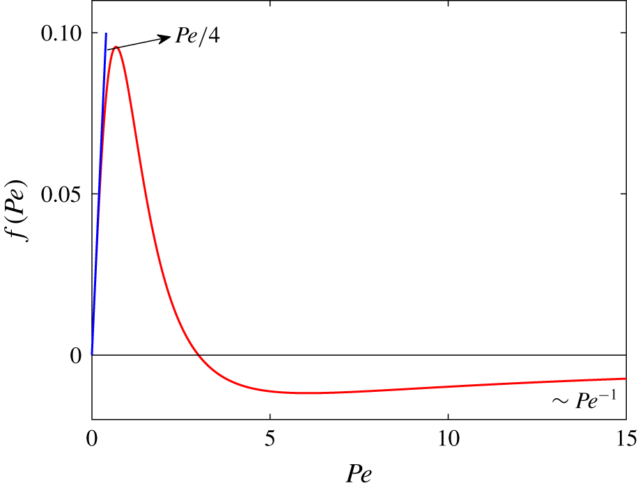
 $Pe$ is given by (3.12), which is plotted in figure 2. From figure 2, we find that the linear fit derived from (3.13) (
 $f(Pe)=Pe/4$), provides an accurate estimate for Péclet numbers up to 0.35. We also observe that
 $|\,f(Pe)|$ has a maximum value of
 ${\sim}0.1$. Additionally, as the spatial scale on which the magnitude of the stratifying agent varies (
 $\unicode[STIX]{x1D707}_{\infty }/\unicode[STIX]{x1D6FE}$) is expected to be much larger than the length scale of the swimmer (
 $1/k$), we expect the value of
 $\unicode[STIX]{x1D6FC}$ to be much smaller than unity. Hence, the contribution of
 $V_{viscous}$ to the swimming velocity (refer to (4.1)) is expected to be at least two orders of magnitude smaller compared to the homogeneous counterpart (refer to (3.11)). Nevertheless, by focusing on the contribution of the viscosity-gradient-induced velocity, we can obtain important insights regarding the preferential bias of the swimmers towards high/low-viscosity regions.
We observe that, for small Péclet numbers ( $0<Pe<3$), the effect of the viscosity gradient is to propel the swimmer in the positive
 $y$ direction. However, for large Péclet numbers (
 $Pe>3$), the viscosity gradient pushes the swimmer in the negative
 $y$ direction. The linear dependence of
 $V_{viscous}$ on
 $\unicode[STIX]{x1D6FC}$ implies that if the direction of the viscosity gradient is reversed, the effect of the viscosity gradient on the swimming velocity would be reversed. Hence, for small (large) Péclet numbers, the effect of the viscosity gradient is to propel the swimmer towards regions of low (high) viscosity.
Contribution of the viscosity gradient to the swimming velocity for  $\unicode[STIX]{x1D6FC}=1$. The blue line represents the linear fit at small Péclet numbers derived from (3.13).

In our analysis, we have assumed a surface transverse wave travelling in the negative  $y$ direction. However, we can show that for a wave travelling in the positive
 $y$ direction, the expression for
 $V_{viscous}$ remains the same. This implies that the contribution of the viscosity gradient to the swimming velocity is independent of the direction of the travelling wave generated by the swimmer. We can now conclude that, in the presence of viscosity gradients, the swimming sheet would prefer regions of low (high) viscosity for small (large) Péclet numbers. Consequently, our analysis shows that the swimming sheet shows negative viscotaxis for
 $0<Pe<3$ and positive viscotaxis for
 $Pe>3$. As opposed to the previous studies, which attributed the viscotaxis response to the speculative existence of viscoreceptors (Petrino & Doetsch Reference Petrino and Doetsch1978; Daniels et al. Reference Daniels, Longland and Gilbart1980; Sherman et al. Reference Sherman, Timkina and Glagolev1982; Takabe et al. Reference Takabe, Tahara, Islam, Affroze, Kudo and Nakamura2017), our work shows that swimmers might exhibit a viscotaxis behaviour purely based on hydrodynamic effects.
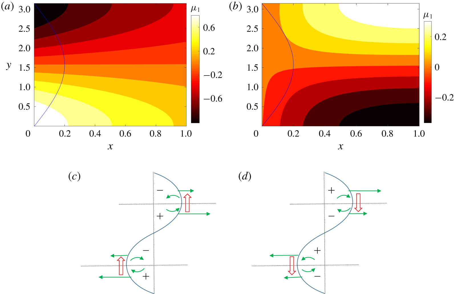
The hydrodynamic mechanism for such a behaviour can be explained by focusing on the distribution of the viscosity in the vicinity of the swimmer. Figure 3(a,b) shows the variation of the disturbed viscosity near the sheet’s crest (shown in blue) for the cases of low Péclet number ( $Pe=0.01$) and high Péclet number (
 $Pe=100$), respectively. For low Péclet numbers, we find that the value of the disturbed viscosity (
 $\unicode[STIX]{x1D707}_{1}$) is positive in the lower half of the sheet surface (
 $0<y<\unicode[STIX]{x03C0}/2$) and negative in the upper half (
 $\unicode[STIX]{x03C0}/2<y<\unicode[STIX]{x03C0}$). However, for large Péclet numbers, this trend is reversed and even the magnitude of the viscosity is smaller. As the sheet retreats back towards its undeformed configuration, viscous forces are generated in the fluid which resist the velocity gradients. The direction of these viscous forces is shown by the green arrows in figure 3(c,d). For low (high) Péclet numbers, the lower (upper) half of the sheet’s crest will experience more viscous resistance due to the higher fluid viscosity. These regions are shown by the longer green arrows in figure 3(c,d). This asymmetric distribution of the viscous forces creates a vortical fluid flow around the sheet’s crest which propels the sheet (red arrows indicate the direction of propulsion). We note that the direction of the vortical flow reverses at high Péclet numbers, which causes the contribution of the viscosity gradient to the swimming velocity to be negative for high
 $Pe$ (refer to figure 2).
Distribution of the disturbed viscosity ( $\unicode[STIX]{x1D707}_{1}$) for (a)
 $Pe=0.01$ and (b)
 $Pe=100$. Hydrodynamic mechanism describing the contribution of viscosity gradients to the sheet’s motion for (c)
 $Pe=0.01$ and (d)
 $Pe=100$. The ‘
 $+$’ sign indicates a positive value for the disturbed viscosity and the ‘
 $-$’ sign indicates a negative value for the disturbed viscosity; green arrows represent the viscous forces in the fluid; and red arrows represent the contribution of the vortical flow (shown in green) to the propulsion of the swimmer.

Studies have shown that diffusive transport is significantly more important compared to advective transport within the mucous layer (for example, Mirbagheri & Fu (Reference Mirbagheri and Fu2016) reported a Péclet number of  $10^{-3}$ for transport of ammonia in the gastric mucous layer, and Lewis, Keener & Fogelson (Reference Lewis, Keener and Fogelson2017) reported a Péclet number of
 $10^{-2}$ for transport of hydrogen ions within the gastric mucous layer). Additionally, diffusion is the predominant transport process in biofilm cells, where the Péclet number is of the order of
 $10^{-3}$ (Stewart Reference Stewart2012). For such small Péclet numbers observed in mucous layers or biofilms, our analysis predicts that the swimmers would prefer regions of low viscosities.
Additionally, when our analysis is extended for large viscosity gradients, the contribution of the viscosity gradient dominates the homogeneous contribution and our theory predicts accumulation of the swimmers in regions of low or high viscosity depending on the Péclet number corresponding to the transport of the stratifying agent. Stehnach (Reference Stehnach2019) observed that swimming biflagellates accumulate in the high-viscosity region for longer flagella lengths. For their experimental analysis, the length scale is  $l_{c}\sim 10^{-5}~\text{m}$, the velocity scale is
 $u_{c}\sim 10^{-4}~\text{m}~\text{s}^{-1}$ and the diffusion coefficient is
 $c\sim 10^{-11}~\text{m}^{2}~\text{s}^{-1}$, which results in a Péclet number of
 $Pe\sim 100$. If we assume that the swimming sheet model can be used to provide an insight into the motion of C. reinhardtii in a viscosity-stratified fluid, then from our analysis we can predict that, for
 $Pe\sim 100$, the swimmers would accumulate in the high-viscosity regions as observed in their experiments.
4.2 Power expenditure and swimming efficiency
The power expended by the swimmer is given by
 $$\begin{eqnarray}P=\int _{S(t)}\boldsymbol{n}\boldsymbol{\cdot }\unicode[STIX]{x1D748}\boldsymbol{\cdot }\boldsymbol{u}\,\text{d}S=\int _{V(t)}(\unicode[STIX]{x1D735}\boldsymbol{\cdot }\unicode[STIX]{x1D748})\boldsymbol{\cdot }\boldsymbol{u}\,\text{d}V+\int _{V(t)}2\unicode[STIX]{x1D707}\unicode[STIX]{x1D640}\boldsymbol{ : }\unicode[STIX]{x1D640}\,\text{d}V.\end{eqnarray}$$
Here,  $\unicode[STIX]{x1D748}$ and
 $\unicode[STIX]{x1D640}$ are the stress tensor and the rate-of-strain tensor, respectively;
 $S(t)$ represents the surface of the swimmer; and
 $V$ represents the fluid volume which is bounded by the sheet surface and extends to infinity. The rate-of-strain tensor can be written as
 $\unicode[STIX]{x1D640}=\frac{1}{2}(\unicode[STIX]{x1D735}\boldsymbol{u}+\unicode[STIX]{x1D735}\boldsymbol{u}^{\text{T}})$, where
 $\boldsymbol{u}=(u_{1},v_{1})$ represents the first-order velocity field. As inertia is assumed to be negligible in our work,
 $\unicode[STIX]{x1D735}\boldsymbol{\cdot }\unicode[STIX]{x1D748}=0$, and the power dissipation is given by
 $$\begin{eqnarray}P=\int _{V(t)}2(\unicode[STIX]{x1D707}_{\infty }-\unicode[STIX]{x1D6FE}y+\unicode[STIX]{x1D707}^{\prime })\unicode[STIX]{x1D640}\boldsymbol{ : }\unicode[STIX]{x1D640}\,\text{d}V.\end{eqnarray}$$
Using the expression for the first-order velocity and viscosity fields derived in (3.2) and (3.3), we find that
 $$\begin{eqnarray}\int _{V(t)}\unicode[STIX]{x1D707}_{1}^{\prime }\unicode[STIX]{x1D640}\boldsymbol{ : }\unicode[STIX]{x1D640}\,\text{d}V=0.\end{eqnarray}$$
We can now split the power expenditure into two components,  $P_{h}=2\unicode[STIX]{x1D707}_{\infty }\int _{V(t)}\unicode[STIX]{x1D640}\boldsymbol{ : }\unicode[STIX]{x1D640}\,\text{d}V$ and
 $P_{v}=2\unicode[STIX]{x1D6FE}\int _{V(t)}y\unicode[STIX]{x1D640}\boldsymbol{ : }\unicode[STIX]{x1D640}\,\text{d}V$ which denote the magnitude of the mean power expended by the swimmer in a homogeneous fluid of viscosity
 $\unicode[STIX]{x1D707}_{\infty }$ and the contribution of the ambient viscosity gradient to the power expenditure, respectively. We substitute the expression for the first-order velocity fields and evaluate the integrals to obtain the following expression:
 $$\begin{eqnarray}P_{v}=\unicode[STIX]{x1D6FC}\unicode[STIX]{x03C0}P_{h}.\end{eqnarray}$$
We find that the viscosity-gradient-induced power expenditure increases with  $\unicode[STIX]{x1D6FC}$. This is expected, as the swimmer dissipates more energy in the fluid for larger ambient viscosity gradients.
Lighthill (Reference Lighthill1952) defined swimming efficiency as the ratio of external power required to move the swimmer at a constant velocity to the power expended by the swimmer. This definition is commonly used in the literature to represent the hydrodynamic efficiency of undulating sheets (Li & Ardekani Reference Li and Ardekani2015; Dandekar et al. Reference Dandekar, Shaik and Ardekani2019). We use this definition to quantify the hydrodynamic efficiency of the swimmer in a viscosity-stratified fluid. Hence, we obtain
 $$\begin{eqnarray}\unicode[STIX]{x1D702}\propto \frac{V^{2}}{P}.\end{eqnarray}$$
Here,  $V$ is the swimming velocity and
 $P$ is the mean power expended by the swimmer over one time period. We use this formula to compare the hydrodynamic efficiency of the swimmer in a homogeneous and a viscosity-stratified fluid. Using (3.11) and (4.3), we obtain
 $$\begin{eqnarray}\frac{\unicode[STIX]{x1D702}}{\unicode[STIX]{x1D702}_{h}}=\frac{4(\frac{1}{2}+\unicode[STIX]{x1D6FC}f(Pe))^{2}}{1+\unicode[STIX]{x1D6FC}\unicode[STIX]{x03C0}}.\end{eqnarray}$$
As  $f(Pe)\sim O(0.01)$ (refer to figure 2), the above expression simplifies to
 $$\begin{eqnarray}\frac{\unicode[STIX]{x1D702}}{\unicode[STIX]{x1D702}_{h}}\sim \frac{1}{1+\unicode[STIX]{x1D6FC}\unicode[STIX]{x03C0}}.\end{eqnarray}$$
We thus infer that increasing viscosity gradient decreases the hydrodynamic efficiency of the swimmer, as the swimmer expends power at a faster rate compared to a change in the swimming velocity.
5 Conclusion
In this work, we theoretically investigated the motion of a swimming sheet immersed in a viscosity-stratified fluid. We used a regular perturbation expansion approach with the small parameter as  $bk$, which signifies the ratio of the wave amplitude to the wavelength. We derived an expression for the swimming velocity of the sheet up to second order in the small parameter.
We found that, in the presence of viscosity gradients, the velocity of the sheet depends on the viscosity gradient in the ambient fluid and the Péclet number. In particular, for small Péclet numbers, the viscosity gradient leads to motion of the sheet towards regions of low viscosity (negative viscotaxis), and for large Péclet numbers, the sheet favours high-viscosity regions (positive viscotaxis). Hence, based on our work, we find that purely hydrodynamic effects might be responsible for the viscotaxis phenomena. Our theory predicts that, for swimmers translating in inhomogeneous mucous environments or biofilms, which are usually dominated by diffusion of the stratifying agent, the small Péclet number causes them to prefer regions of lower viscosities. By extending our analysis for large viscosity gradients, we can predict the experimentally observed accumulation of wild-type C. reinhardtii near high-viscosity regions. Additionally, we derived an expression for the power expenditure and the hydrodynamic efficiency of the swimmer in the presence of viscosity gradients.
Acknowledgements
This publication was made possible due to support from NSF (grant no. 1700961). R.D. is grateful for a Frederick N. Andrews Fellowship for financial support.
Declaration of interests
The authors report no conflict of interest.