I. INTRODUCTION
Although the direct conversion of heat flow into electrical power based on the occurrence of thermovoltage from a temperature difference known as the Seebeck effect, and likewise the inverse Peltier effect, which is the transport of heat directly linked to a current flow, have been discussed for a long time, there has been great progress in understanding these phenomena from a more microscopic point of view.Reference Behnia, Jaccard and Flouquet1, Reference Behnia2 More recently the thermoelectric (TE) spin transfer in textured magnetsReference Kovalev and Tserkovnyak3 and the TE effect of Dirac fermions in graphene has been studied numerically.Reference Zhu, Ma, Sheng, Liu and Sheng4 Despite the effort in microscopic modeling, the application of linear thermodynamics of irreversible processes within a continuum approach is still under debate, especially for graded and segmented TE elements. They are characterized by locally nonconstant transport coefficients like the Seebeck coefficient, the electrical and thermal conductivities (see, e.g., Refs. Reference Kuznetsov5 and Reference Müller, Zabrocki, Goupil, Snyder, Seifert and Rowe6). One aim of this study is to improve the performance of thermogenerators (TEGs) that are exposed to a large temperature difference. In 1909 AltenkirchReference Altenkirch7 had already calculated the efficiency of a thermopile concerning the material properties that are needed to build practical devices. He provided the first evidenceReference Altenkirch7, Reference Altenkirch8 that good TE materials should have a large Seebeck coefficient S, a high electrical conductivity σ (low electrical resistivity) to minimize Joule heat, and a low thermal conductivity κ to retain heat at the junctions and maintain a large temperature gradient. Later these qualitative aspects were embodied in the material figure of merit z = S 2σ/κ.Reference Ioffe9 Note that there are correlations between the material coefficients like the Wiedemann–Franz law (connecting the electronic part of thermal conductivity and electrical conductivity) or Mott’s formula, which links the Seebeck coefficient and electrical conductivity.Reference Jonson and Mahan10–Reference Ashcroft and Mermin12 For metals the development of efficient TEGs can be traced to the thorough studies of the PbS–ZnSb compounds that were aimed to develop better material properties.Reference Telkes13, Reference Wood14 Even the description of a solar TEG is related to Refs. Reference Telkes15–Reference Telkes17. The breakthrough of the theoretical description was due to Onsager’s formulation of the physical principles underlying irreversible phenomena. This approach offered the basis for the theoretical description of TE effects.Reference Onsager18, Reference Onsager19 The usage of semiconductors as TE materials led to a revival of TEs in the late 1950s that was due to IoffeReference Ioffe9 and Goldsmid.Reference Goldsmid and Douglas20 Because there had been no significant advances in improving the device efficiency or materials’ figure of merit after the mid-1960s, the interest in thermoelectricity declined under the weight of inflated hopes after a very active period of investigations. The basic research in TEs stagnated for 30 years after that, as breakthroughs in the field decelerated; meanwhile some materials and commercial uses were still developed. New ideas and materials in the mid-1990s brought back TEs from niches into the focus of research. The search for green technologies, e.g., converting waste heat generated by car engines into usable power, pushes scientists to pick up “old” effects with new classes of materials exhibiting higher TE figures of merit to create practical applications using the advantages of TE power generation.Reference Rowe21, Reference Rowe22 A nice overview of different applications is given by Riffat and Ma.Reference Riffat and Ma23 Especially, the advantages of TE devices made them capable for applications in wide areas such as military, aerospace, measurement devices, and industrial or commercial products. Thus, TE solid-state equipment has no mobile parts and therefore needs much less maintenance. Other benefits are due to long-term steady-state operation time and an ecological point of view as the absence of chlorofluorocarbons. Otherwise, the efficiency of TE devices is lower in comparison to conventional coolers and engines. Nevertheless, in the age of global warming all possible ways of saving “waste” energy are welcome, independent of whether its origin is an industrial one or comes from such units like private cars, even if one should not overestimate their amount by using TE effects.Reference Vining24 The efficiency of today’s TE devices has to be improved not only by optimizing the material’s performance itself but also by taking advantage of any option provided by special material design or functional grading of the material. To develop such high-performance functionally graded materials (FGM), the role of nanotechnology has been increased drastically.Reference Rowe21, Reference Rowe22, Reference Shiota and Miyamoto25 There are different ways to model TE modules, depending on the length scale one is interested in. Whereas on a macroscopic scale the nonequilibrium thermodynamics attributable to Onsager is applicable,Reference Onsager18, Reference Onsager19 on a mesoscopic scale and a microscopic scale the Boltzmann equation or a nonequilibrium quantum approach are appropriate tools.Reference Rowe22, Reference Tritt26 In this article we focus on a continuum approach at a macroscopic scale. The TE material properties are in general both temperature and spatially dependent quantities,Reference Domenicali27–Reference Lienhard and Lienhard30 although especially in engineering the focus is preferentially set on the determination of the temperature dependence of the material properties. This material’s dependence on both implies two kinds of homogeneity (or inhomogeneity). On the one hand, a physically inhomogeneity is possible, i.e., the material’s properties are temperature dependent; on the other hand, there is a chemical inhomogeneity in which you find the material’s properties position dependent in a sample.Reference Domenicali27, Reference Domenicali28, Reference Schilz, Müller, Helmers, Kang, Noda and Niino31 If mainly this T dependence is considered, one can express the material properties as spatial profiles over the length of a TE leg equivalently, as there is a steady temperature profile T(x) available for any performance parameter in the one-dimensional (1D) steady state. Exemplarily, for the Seebeck coefficient, the spatial profile is then given by S(x) = S[T(x)]. It is well accepted that the material properties, in particular those of semiconductors, strongly depend on the carrier concentration that can be influenced by appropriate doping agents or a variation of the chemical composition.Reference Ioffe9, Reference Egli32, Reference MacDonald33 Monitoring the carrier concentration opens the possibility of attaining a spatially dependent material, even if the temperature dependency is neglected. In this paper the material properties are assumed to be explicitly temperature independent (i.e., physically homogeneous) but spatially dependent (i.e., chemically inhomogeneous) to point out the quantitative effects of spatially dependent properties on, in particular, the performance parameters of a TEG with the efficiency η or the electrical power P el. By that it is felt that these assumptions will provide an accurate mathematical model of the physical system while getting analytical solutions, yielding a better physical insight into the effect on the performance parameters concerning spatially dependent TE materials. Linear spatial profiles are among the basic approaches to finding the profiles that deliver optimum performance. The linear properties model (LPM) presented, as well as the constant properties model (CPM), i.e., a totally (chemically and physically) homogeneous material first considered for performance investigations by Ioffe,Reference Ioffe9 is limited in comparison with really measured temperature dependent material. However, it can provide hints for optimized stacking schemes. Investigations similar to the present ones have already been performed.Reference Ybarrondo34, Reference Ybarrondo and Sunderland35 Although these authors were successful in getting an analytical solution for the evolving temperature profile, the performance could not be determined quantitatively there because of the lack of suitable computation tools. Therefore, we revisit the corresponding solutions in particular to gain information about the influence of the slope of the material parameters on the performance. Furthermore, we calculate the corresponding optimal values in the particular case of linear spatial profiles as an example of FGM. In the present paper, we are able to compute the temperature profile T(x) analytically within a “model-free setup” directly from the 1D thermal energy balance. It is assumed that all material profiles are independent of each other and have a linear spatial profile that is freely variable. The optimum current density and the optimum slopes for the profiles can be determined from the maximum of the global performance parameter under consideration while varying the current and slope. For arbitrary continuous and monotonous gradient functions of the material profiles S(x), σ(x), and κ(x), the calculation of the temperature profile has been done numerically up to now by either a 1D TE finite element method code or the algorithm of multisegmented elements.Reference Müller, Walczak, Seifert, Stiewe, Karpinski and Tritt36–Reference Müller, Karpinski, Wu, Walczak, Seifert and Rogl38 Our analytical solution offers another reference, in addition to CPM, to test numerical procedures like that. Moreover, our results could also be the basis of a new multisegment algorithm based on LPM instead of CPM. Likewise, it can be used as the starting point for finding more generally shaped optimum profiles of the material properties. In the context of optimizing the performance by using graded material, the work of Bian et al. should be mentioned.Reference Bian and Shakouri39, Reference Bian, Wang, Zhou and Shakouri40 In their calculations the power factor f = S 2σ was assumed to be constant, together with a high and constant thermal conductivity for which the end result is small overall temperature differences along the TE element.
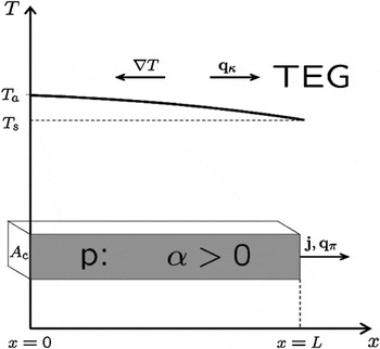
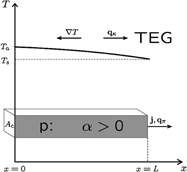
Within the framework of a 1D steady-state model, our analysis is based on a single p-type TE element with fixed length L and cross-sectional area A c as part of a TEG.Reference Seifert, Müller, Walczak and Rogl37, Reference Snyder and Rowe41, Reference Seifert, Müller, Snyder and Walczak42 A sketch of our model is shown in Fig. 1. Obviously the model will not capture all details of real materials such as the contact resistance, the nonparallel current flow, any heat loss perpendicular to the flow direction, and any heat loss due to convection or radiation. In this context, the following investigations are intended primarily for an “ideal” TE system.Reference Snyder and Rowe41 Note that in this 1D description the spatial gradient is of course in the axial direction of the TE element (the direction of the heat flow and electrical current). With that we have the configuration of a longitudinal TEG.Reference Gryaznov, Moizhes and Nemchinskii43
One-dimensional setup of the TE element; notation of the vectors according to Eq. (1).

II. 1D THERMAL ENERGY BALANCE
TE effects are caused by the coupling of heat and charge transport that can be described within the framework of the linear response theory. For a detailed consideration, see Refs. Reference Onsager18 and Reference Onsager19. In particular for applications to TEs, see Refs. Reference Domenicali27, Reference Domenicali28 and Reference de Groot and Mazur44–Reference Mahan46. This approach is also denoted as Onsager–de Groot–Callen theory.Reference Onsager18, Reference Onsager19, Reference de Groot and Mazur44, Reference Onsager47–Reference Callen50 The transport of heat and charge is described by the corresponding current densities q (heat flow, heat flux) and j (electrical current density), respectively, which provide under isotropic conditions the linear constitutive relations


where E is the electric field, qκ is the Fourier heat flux, qπ is the Peltier heat flux, and T is the temperature. (Normally, Q denotes the heat in units of 1 J, whereas with  the heat transfer rate or heat flow in units of 1 W is meant. For the sake of simplicity the dot is sometimes ommitted. Often used is the heat flux, which is the heat transfer rate per cross-sectional area
 in units of 1 W/m2.) Note that the Peltier heat flux has to be distinguished from what is phenomenologically known as the Peltier heat as occurring at a material transition; the latter represents just the divergence, i.e., the local rate of change of the first. The Peltier flux is treated here as a flux of thermal energy, although the energy transport does not actually take place as a transport of heat but of potential energy of the charge carriers. However, this energy can be made thermally apparent locally by introducing an (infinitesimally) thin layer with a vanishing Seebeck coefficient. The parameters S, σ, and κ are the aforementioned material parameters that generally depend on the temperature and the spatial coordinate. Under steady-state conditions the conservation of charge and energy leads to


Assuming a 1D setup with constant electrical current density j = j ex, Eq. (2a) is obviously fulfilled. From Eq. (1a) one easily deduces
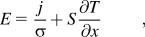
with the first term representing the voltage drop because of the material’s resistivity but the second representing an additional field due to the evolving thermovoltage. Inserting Eq. (1b) into Eq. (2b) and using Eq. (3), the local thermal energy balance reads as

Similar calculations can be found in Refs. Reference Domenicali28, Reference Mahan46, and Reference Seifert, Ueltzen and Müller51–Reference Harman and Honig53. Equation (4) is just a 1D representation for isotropic material of Domenicali’s 3D expression of the production of heat in an inhomogeneous, anisotropic medium, crystalline or otherwise (steady state).Reference Domenicali27, Reference Domenicali28 The general material’s dependence on the temperature T and the position r, e.g., S = S[r,T(r)], leads to a split-up of the derivative concerning the Peltier–Thomson term:
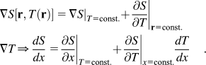
This split-up due to the chain rule corresponds to different physical heat fluxes: the (distributed) Peltier heat  and the Thomson heat
 . Buist made the distinction between extrinsic and intrinsic Thomson heat for both terms.Reference Buist and Vedernikov54 In the 3D case there could be a third term if the electrical current density is spatial dependent, representing the so-called Bridgman heat. For the 1D case the steady-state condition ∇·j = 0 leads to ∂j(x)/∂x = 0, i.e., j = const. The peculiarity of that equation is because the TE properties are playing a role twice here: first, thermal energy is absorbed or released according to the gradient of the Peltier coefficient ST (last term on the left side), but second, (right side) as a local energy conversion from or into electricity because of the current driven by or against the thermovoltage. Note that Eq. (4) can be understood in different ways because of the assumed type of the dependence of the material coefficients. If the parameters S, σ, or κ depend only on the temperature T but not explicitly on the spatial coordinate, i.e., we have a chemically homogeneous but physically inhomogeneous material, then Eq. (4) adopts the form

which is a nonlinear differential equation for the unknown temperature profile T(x). Here we have introduced the Thomson coefficient  . The differential equation has to be supplemented by boundary conditions. In 1D TE problems, Dirichlet boundary conditions can be applied, i.e., two fixed temperatures at the x = 0 and x = L or mixed boundary conditions where a heat flux is given at x = 0. Throughout this paper, T a = T(x = 0) is the temperature at the heat-absorbing side (hot side for TEG), whereas T s denotes the heat sink temperature that is in many practical situations fixed close to room temperature. If the material parameters are supposed to be temperature dependent, averaged parameters can be defined by
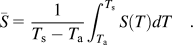
The temperature averages of further material parameters are defined in an analogous manner.
In the 1D steady state there is a one-to-one correspondence of the temperature T and the position x if the temperature profile is a continuous and strictly monotonous one. This especially applies for maximum efficiency and maximum power output of a TEG if constant or real, temperature dependent, material properties are considered. Then, there exists the inverse function x(T) to T(x). If these conditions are fulfilled, Eq. (5) can be transformed into

with ρ(x) = 1/σ(x), where we presume spatial material profiles S(x), σ(x), and κ(x) (see, e.g., Refs. Reference Bian and Shakouri39, Reference Mahan46, Reference Seifert, Ueltzen and Müller51, Reference Mahan52, and Reference Seifert, Müller and Walczak55). Now the temperature dependence of the material parameters can be expressed by their spatial dependence leading to

with S(x) = S[T(x)]. As the function LT′(x)/(T s – T a) varies around unity, both the temperature average and the spatial average turn out to be close together for moderate gradients, where the spatial average will be defined as 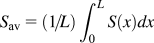 . As a consequence, we get for the Seebeck coefficient
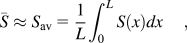
where the index “av” denotes the spatial average according to Eq. (7). Note that  holds exactly for linear temperature profiles and in the CPM case, where the material properties are supposed to be constant and with it independent of the temperature and the position in the TE element. Naturally, Eq. (6) can also be used as an independent differential equation when the spatial dependence of the material parameters S(x), σ(x), and κ(x) are the center of interest; see, for instance, Refs. Reference Ybarrondo34, Reference Ybarrondo and Sunderland35, and Reference Müller, Karpinski, Wu, Walczak, Seifert and Rogl38. Let us emphasize that, in contrast to Eq. (5), the differential equation Eq. (6) with spatially dependent material profiles is linear in T. This enables us to search for analytical solutions based on the principle of superposition.
In FGMs the whole set of material parameters may depend not only on the temperature but also on the local material quality that can be practically the composition of an alloy or the concentration of a dopant. For example, let us consider a single doped material or an alloy characterized by the concentration c(x). Thus, the gradient of the Seebeck coefficientReference Harman and Honig53S can be written as

In 1D the gradient of the Seebeck coefficient reads ∇S = dS/dx ex if the single element profiles c(x) and T(x) are known, i.e.,

Spatial material profiles may have a new quality: taking all local (implicit) dependencies into account, the graded TE material can be spatially dependent even under isothermal conditions. Note also that noncontinuously graded (i.e., segmented) elements are considered as FGM because they lead to the same functional effect.
III. ANALYTICAL SOLUTION FOR LINEAR SPATIAL PROFILES
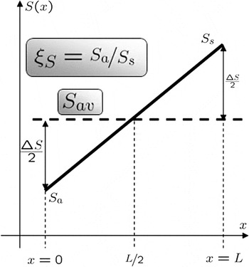
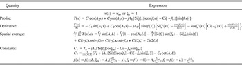
Usually, a linear Seebeck profile (see Fig. 2) over the length of a TE element (0 ≤ x ≤ L) is given by

Spatially linear profile of the Seebeck coefficient throughout the TE element;  and


where S a = S(x = 0) and S s = S(x = L) denote the Seebeck values at the boundaries. For our purpose we just take another description because we want to fix the (spatial) average of the Seebeck coefficient  to compare the results of the LPM with those of the CPM. Further, we define ξS = S a/S s as the ratio of the boundary values of the Seebeck coefficient. Then, Eq. (8) can be transformed into

with

Analogously, the thermal and electrical conductivities κ(x) and σ(x) can be defined containing the appropriate averages and ratios, κav, σav,  , respectively. In addition, we use the abbreviations

where y stands for S, κ, or σ.
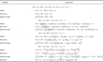
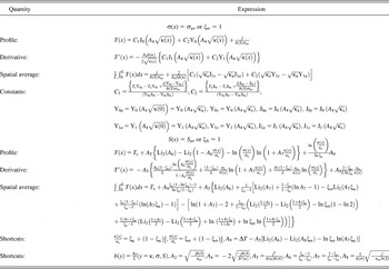
The thermal energy balance Eq. (6) with the profiles defined according to Eq. (9) is an inhomogeneous differential equation having an analytical solution in the form of Bessel functions (see Appendix A). It is common knowledge that these functions have been found in a wide variety of physical problems. For an overview of this and the properties of these functions, see Refs. Reference Abramowitz and Stegun56–Reference Mathews and Meissel60. The solution of the boundary value problem for the temperature profile for given ratios ξκ, ξS, and ξσ can be found as a sum of the general solution of the homogeneous equation and a particular solution of the inhomogeneous equation, see Appendix A and Tables I-III.

where Y0 and J0 are the Bessel functions, κ(x), σ(x) are taken as defined in Eq. (9). The free constants C 1 and C 2 can be fixed by boundary conditions. Particular solutions for different variants of given linear profiles are listed in Tables I-III.
Special cases I.

Spacial cases II.

Spacial cases III.

IV. PERFORMANCE PARAMETERS OF A TEG AND CPM
Once having calculated T(x), all performance parameters of interest can be determined as a function of the electrical current density j. In this paper we are concentrating on the electrical power P el and on the efficiency η of a TEG, therewith continuing previous investigations on graded TEGs.Reference Ybarrondo and Sunderland35, Reference Ure and Heikes61–Reference Seifert, Zabrocki, Snyder and Müller65
In a 1D setup, the electrical power is given byReference Seifert, Müller and Walczak55
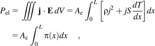
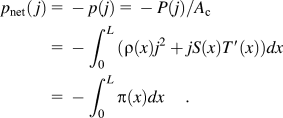
where π = j· E is the electrical power in a volume dV or the differential electrical power.Reference Seifert, Zabrocki, Snyder and Müller65 The power output of a TEG is defined here according to thermodynamic rules: quantities input to the system are positive. Hence, the net power output density (net electrical power output per cross-sectional area A c) is
Finally, the efficiency of a TEG is defined as the ratio between the electrical power output and the entering thermal power Q a,

where q a is the absorbed thermal power density at x = 0 [see Eq. (1b) and Fig. 1].
Many of the previous works are related to the CPM (i.e., totally homogeneous material). For an approximation you can take the averaged values of the material properties, which means S(x) = S av, σ(x) = σav, and κ(x) = κav, and calculate the performance in the framework of CPM with these values. Note that there is another possibility of taking the constant coefficient for the thermal energy balance into account, e.g., by averaging the Thomson coefficient τ instead of the Seebeck coefficient, which is called the method of averaged coefficient (see Ref. Reference Harman and Honig53, p. 276). In the following we will concentrate on the CPM and calculate the performance parameters from the resulting parabolic temperature profile
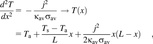
leading to the net power output density

which is nothing else than the difference between the TE voltage and the ohmic voltage drop. A straightforward calculation gives the efficiency η as a function of the electrical current density j (see Ref. Reference Seifert, Müller and Walczak55):
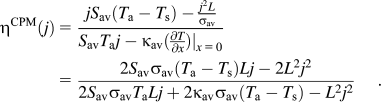
An optimization of the performance parameters in the case of CPM due to j is a classical extreme value task. The external parameters like the geometry with L and A c as well as the boundary temperatures T a and T s are kept fixed during this optimization. From the solution of the equations  and
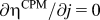 the optimum values for the current densities, where you find maxima for the performance parameters, are calculated as
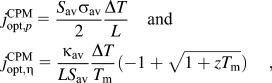
where ΔT = T a – T s, T m = (T a + T s)/2, and  are the respective temperature difference, the (arithmetic) average temperature, and the material’s figure of merit. Setting these optimum current densities in Eq. (14) and Eq. (15), respectively, leads directly to the well-known formulae of maximum performance parameters:
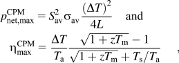
see, e.g., Refs. Reference Altenkirch7–Reference Ioffe9. Note that these formulae are in a strict sense only valid for constant material properties, although they are often used as an approximation for temperature dependent materials. For those materials the usage of an effective figure of merit is supposed, especially for large temperature differences ΔT. Reference Müller, Zabrocki, Goupil, Snyder, Seifert and Rowe6, Reference Kaliazin, Kuznetsov and Rowe29, Reference Moizhes66–Reference Muto, Kraemer, Hao, Ren and Chen70
V. TEG PERFORMANCE OPTIMIZATION VIA LINEAR GRADING
It is not the aim of this paper to discuss all optimization variants based on given linear profiles. In general, it is possible to search for the global maximum and the related optimum current of the performance parameter under consideration by adjusting the slope of the material profile via the ratios ξκ, ξS, and ξσ with respective fixed spatial averages κav, S av, and σav.
Considering the net power output density first, we find Eq. (18) for a constant electrical conductivity (ξσ = 1), which is supposed to be in the vicinity of the maximal performance, after integration by partsReference Zabrocki, Müller and Seifert71:

In Eq. (18) the grading of ξκ enters through the spatial average 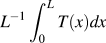 . The efficiency can be calculated with Eqs. (12), (18), and (1b).
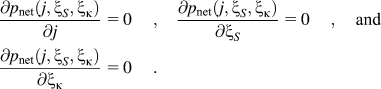
We first discuss the particular case of having only one linear profile for the Seebeck coefficient, where as the conductivities are supposed to be constant (ξS ≠ 1, ξκ = ξσ = 1). For that the material parameters are chosen as S av = 180 μV/K, κav = 1.35 W/m K, and σav = 14·104 S/m exemplarily; and the dimensionless figure of merit is approximately 1 at T = 300 K. For all numerical calculations we suppose an element length L = 5 mm and the boundary temperatures are fixed to T a = 600 K and T s = 300 K, i.e., a temperature difference ΔT = 300 K. In the CPM case the optimal performance parameters  , as well as the optimal current densities are given by Eqs. (16) and (17), whereas for LPM one ends up in a multidimensional extreme value task with a system of equations leading to the optimum current densities j opt and grading parameters ξopt, e.g.,
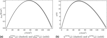
By linear profiles of S both the power output and the efficiency can be increased. As for CPM the optimal parameters are different depending on what has to be optimized, p net or η, but we find the same directions in the optimization strategy. Both TEG performance parameters are displayed in Fig. 3 for a TE element of length L = 5 mm and a fixed temperature difference ΔT = 300K, showing by that the difference between homogeneous and graded material. The results for CPM (i.e., totally homogeneous) and LPM (i.e., linear material profiles) are also compared in Table IV. Using Eqs. (14) and (18) the difference between the power output in the CPM and LPM case can easily be deduced to

Comparison of power output density and efficiency of a CPM, i.e., totally homogeneous, and LPM (graded) element for a TEG element (L = 5 mm, T a = 600 K, T s = 300 K, S av = 180 μV/K, κ av = 1.35 W/m K, σ av = 14·104 S/m) depending on the electrical current density for the optimal parameters ξS ,opt given in Table I.

with mean temperature  and averaged temperature
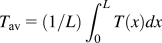 . It is clearly visible from Eq. (19) that two factors have influence on the difference δp net; one factor is the slope of the Seebeck coefficient b(S) = ΔS/L. Note that we have ΔS = 0 in the CPM case and hence a zero difference. A second factor is the deviation of the temperature profile T(x) from a pure linear one. Linear material profiles lead clearly to a nonlinear temperature profile, shifting the spatial average away from the mean of the boundary temperatures and leading to an increasing difference in power output.
Table IV clarifies that graded materials design may imply only a small reserve to improve the performance of a TEG if a constant thermal conductivity is assumed (see also Ref. Reference Seifert, Zabrocki, Snyder and Müller65). The increase of TEG’s power output and efficiency is more pronounced when considering linear profiles S(x) and κ(x) as a further example. The first results were published in Ref. Reference Zabrocki, Müller and Seifert71, demonstrating the ability to exactly evaluate the limiting cases for extreme parameters ξS and ξκ.
Values of the optimum performance parameters for the given material.

VI. CONCLUSIONS
In the present paper we studied transport processes in a continuous medium with local equilibrium. In particular, the paper focused on TE effects as phenomena associated with the simultaneous presence of an electric current and a heat flux. Whereas in the conventional thermodynamics of irreversible processes the transport coefficients are assumed to be at least piecewise constant, we discussed here the case that the TE material parameters offers a spatial dependence. Such a situation is realized in graded and segmented TE elements. In order to optimize the performance of TE elements it is appropriate to search for analytical solutions of the underlying equations. Here we discussed the thermal energy balance in the steady state that results in a linear differential equation of the temperature distribution T(x) when assuming linear varying spatial material parameters in a 1D setup. For this case, we attained the analytical solution in terms of Bessel functions. From here the performance parameters like the electrical power and the efficiency of a graded TEG of fixed length under appropriate boundary conditions are specified exemplarily.
The importance of FGM research to device optimization has appeared particularly attractive for TEGs, because maximum power and maximum efficiency points are close together. The question whether compromise gradient schemes can be found is therefore of importance for the practice. There is hope that the knowledge of optimized linear, spatial profiles will provide a chance to come closer to the optimal material gradients. Of course, it would be beneficial to use the results of the LPM approach for the calculation of real FGM and segmented materials and compare it with experimental results already reported in the literature. However, as the CPM, the LPM is not suitable for a direct comparison to the experiment, especially when operating under great temperature differences. The investigation here should only give qualitative hints about how to do the grading knowing that it is not possible to have the TE material properties all at once linear because the interrelation between them is rather nontrivial. In the experiments there is a concentration on the determination of the temperature dependence of the material properties, because this dependence is unique for a material whereas a position dependence is connected with a particular sample (shape, topology). For an overview of experiments in FGM research, see, e.g., Refs. Reference Kuznetsov5, Reference Müller, Zabrocki, Goupil, Snyder, Seifert and Rowe6, Reference Kaliazin, Kuznetsov and Rowe29, and Reference Kuznetsov, Kuznetsova, Kaliazin and Rowe72–Reference Müller, Drašar, Schilz and Kaysser77. There are few experiments concerning the spatially resolved measurement of TE material properties such as the potential scanning microscope (see, e.g., Refs. Reference Ziolkowski, Karpinski, Platzek, Stiewe, Müller and Rogl78 and Reference Platzek, Karpinski, Drasar and Müller79). Until now the progress in the material science of TE elements has been mainly attributable to simulations and modeling using different numerical methods such as the finite difference method or finite element method; see, e.g., Refs. Reference Kaliazin, Kuznetsov and Rowe29, Reference Müller, Walczak, Seifert, Stiewe, Karpinski and Tritt36–Reference Bian, Wang, Zhou and Shakouri40, Reference Helmers, Müller, Schilz and Kaysser62, and Reference Sherman, Heikes and Ure80–Reference Ebling, Bartholomé, Bartel and Jägle96. Of course, an analytical solution can also be used for testing numerical methods.
ACKNOWLEDGMENTS
The authors are very grateful to G.J. Snyder, California Institute of Technology, and C. Goupil, Laboratoire CRISMAT, Caen, France, for helpful discussions.
APPENDIX A: TRANSFORMATION OF THE THERMAL ENERGY BALANCE AND ITS SOLUTION EXPRESSED IN SPECIAL FUNCTIONS
The thermal energy balance Eg. (2b) can be written in another notation where it shows

with the abbreviations
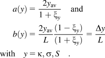
As one easily sees the b gives the appropriate slope, e.g., κ′(x) = b(κ). There is another form of writing the material profiles with the chosen abbreviations, e.g., κ = a(κ)ξκ + b(κ)x. To derive the Bessel equation from the (homogeneous part of the) thermal energy balance [see Eq. (A1)], we used the following substitution:

leading to T″(z) + z –1T′(z) + T(z) = 0 for the homogeneous part of Eq. (A1), which is equivalent to a Bessel equation of order 0 (after multiplying with z 2).
The complete inhomogeneous differential equation can be calculated to

A1. Bessel functions
Some properties of Bessel functions are helpful in calculating the performance parameters,97 f.i. J′0(z) = – J1(z), which leads in our case to

The integral of the Bessel function gives

Analogous relations are found for the Bessel function of the second kind Y0(z).
A2. Sine and cosine integral
Here, Si(x) and Ci(x) are the respective sine and cosine integralReference Weisstein98, Reference Weisstein99
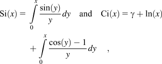
with Euler’s constant γ.
A3. Dilogarithm function
The function Li2(z) is the dilogarithm functionReference Weisstein100 defined as

A more detailed discussion and a number of relations can be found in Refs. Reference Abramowitz and Stegun56–Reference Mathews and Meissel60 and Reference Weisstein97–Reference Watson101 and references therein.