1. Introduction

A prominent feature of Sea-ice drift and especially deformation in both the arctic and antarctic ice pack is the presence of considerable power at the Semi-diurnal timescale (Reference HunkinsHunkins, 1967; hibler and others, 1974; Reference Heil and HiblerHeil and hibler, 2002; Reference Kwok, Cunningham and HiblerKwok and others, 2003). at high latitudes the inertial period is close to the Semi-diurnal period and therefore it is difficult to establish from frequency characteristics alone the most important forcing of the Semi-diurnal power. the two main Sources for these Semi-diurnal oscillations are inertial and tidal. inertial forcing typically arises from wind Stress on the ice–ocean mixed layer, resulting in combined inertial motion of the oceanic boundary layer and ice cover. tidal forcing, on the other hand, affects Sea ice via pressure gradients on the oceanic boundary layer as well as on the ice.

The most recent observational Study of rapid variations in Sea-ice drift and deformation by Reference Kwok, Cunningham and HiblerKwok and others (2003) Shows a general tendency for both ice-drift and Strain-rate ellipses in the central arctic basin to rotate clockwise with periods close to the inertial period. depending on the Sense of the tidally induced drift and deformation, these results tend to be more Supportive of inertial oscillations. a Study on the inertial power by Reference HunkinsHunkins (1967) demonstrated that oscillation amplitude correlates closely with wind magnitude. however, a thorough investigation of the main cause of these oscillations is best conducted with a coupled ice–ocean tidal model. this is especially true of tidal effects; Simply adding tidal forcing to a Stand-alone Sea-ice model will greatly over-amplify tidal effects due to inertial resonance, even with quadratic ice–ocean drag included. by contrast, a carefully coupled ice–ocean model can include physics that are fundamental to high-frequency Sea-ice dynamics. Sea ice floating in the ocean must respond to the Same pressure forces as the oceanic boundary layer. therefore the ice Should not oscillate Significantly differently from the oceanic boundary layer in the absence of internal ice Stresses.

The most direct way to achieve correct coupling of Sea ice and ocean is to ‘dynamically embed’ the ice in the upper oceanic boundary layer. in the Simplest incarnation of this formulation, a ‘slab’ boundary layer can be used (e.g. Reference McpheeMcphee, 1978) whereby the ice is taken to Scale with the integrated boundary layer motion, albeit in a different direction and with a different magnitude. in recent work using a Stand-alone Slab-embedded ice model, Reference Heil and HiblerHeil and hibler (2002) were able to explain a Substantial portion of the Semi-diurnal peak in both Sea-ice drift and deformation obtained from half-hourly autumnal buoy data. the idea of their dynamically embedded model was to remove the unphysical quadratic drag term that is often employed in Stand-alone Sea-ice models (e.g. Steele and others, 1997). use of this term in Stand-alone models can result in Significant artificial damping of the ice motion due to the difference between ice drag and Stresses on the lower portion of the oceanic boundary layer.

The tidal explanation for Semi-diurnal Sea-ice resonance was most notably advanced by Reference Kowalik, Y.Proshutinsky, Johannessen, D.Muench and E.OverlandKowalik and proshutinsky (1994) in an analysis of tidal variability by means of a barotropic tidal model. however, this Study utilized Sea-ice mechanics that only included linear rather than non-linear Shear viscosity and it did not include a detailed comparison with available buoy deformation data. perhaps most importantly in their model, as is the norm in coupled ice–ocean models, the ice was Separated from the ocean in a ‘levitated’ layer above the Sea Surface. by levitated we mean that the modeled Sea ice exchanges momentum with the ocean via ice–water drag and a Sea Surface tilt term only. the Sea ice is not included in the ocean’s mass transport and cannot modify Sea Surface height. not including this Sea-ice transport in the ocean violates archimedes’ principle because modeled Sea ice does not displace water in the ocean and hence it is not floating in the ocean. therefore the Sea ice is effectively levitated above, rather than Suspended in, the oceanic boundary layer, which has particularly deleterious effects when applied to ice–ocean tidal modeling.

It is notable that Reference Mellor and KanthaMellor and Reference Maslowski, Newton, Schlosser, J.Semtner and G.MartinsonKantha (1989) used this levitated formulation for their one-dimensional ice–ocean boundary layer, an application for which it is perfectly consistent because no ice convergence arises. however, in a companion paper, Reference Kantha and L.MellorKantha and mellor (1989) applied it to a two-dimensional ocean circulation model, an application for which it is not physically consistent because ice convergence is present. levitated ice–ocean coupling has Since become commonplace in multidimensional earth System modeling even though it is not physically consistent (e.g. Reference Zhang, Hibler, Steele and A.RothrockPolyakov and others, 1998; Reference Maslowski, Newton, Schlosser, J.Semtner and G.MartinsonMaslowski and others, 2000; wang and others, 2005; Reference Holland, Bitz, Hunke, H.Lipscomb and L.SchrammHolland and others, 2006). in Some climate-system models, Sea ice is part of the atmospheric model component (e.g. Reference Gordon and O’FarrellGordon and o’farrell, 1997) whereby Sea ice remains levitated because its momentum budget is not Solved Simultaneously with ocean circulation.

A different coupling of the ice to the ocean was proposed by Reference Hibler and BryanHibler and bryan (1987) in a diagnostic ice–ocean model. in the Reference HiblerHibler and bryan (1987) coupling, ice is considered to be dynamically embedded into the ocean, and hence the transport of the upper boundary layer of the ocean including the ice transport is taken to be driven by wind Stress and ice interaction. this differs considerably from the levitated mode of water drag, and can be Shown to Significantly modify the vorticity balance, especially in coastal regions, Sometimes even changing the Sign. while using the concept of an embedded formulation, Reference HiblerHibler and bryan (1987) nevertheless utilized a Solution for the ice Separate from the rigid-lid ocean model and then calculated the wind Stress less the ice interaction Separately. in more detailed investigations of variations of this coupled ice–ocean model of the arctic ocean (Reference Hibler and ZhangHibler and zhang, 1995; zhang and others, 1998), it was found that this Separate formulation leads to instabilities at the inertial period in the coupled model, requiring damping of the inertial variability in the upper oceanic boundary layer for Stability. this damping procedure was Subsequently used in formulations of this model at a variety of Scales by zhang and others (1998).

A variation on the dynamically embedded formulation has been built into versions of the geophysical fluid dynamics laboratory (GFDL) ocean model (Reference Griffies, J.Harrison, C.Pacanowski and RosatiGriffies and others, 2004). this model includes a Separate layer for Sea ice in the ocean transport equations. consequently the net ice and ocean transport obeys the Reference Hibler and BryanHibler and bryan (1987) integrated result when the top layer of the ocean and the ice layer are vertically integrated. in practice these models do not Solve the ocean barotropic equations Simultaneously with the ice mechanics. however, by allowing Slip between the ice and the rest of the oceanic boundary layer these models prevent instabilities from occurring without numerical damping of the inertial oscillations (personal communication from S.m. griffies, 2007).

The original embedded formulation of Reference Heil and HiblerHeil and hibler (2002) was designed to remove damping in Stand-alone Sea-ice models. it was also envisioned as an instrument to develop a consistent formulation of a coupled ice–ocean tide model. in this paper, we make Such an extension. moreover, to make the current work more directly applicable to climate-scale ocean model Simulations, we formulate this in a typical b-grid free-surface ocean model with a Somewhat novel Simultaneous Solution procedure to insure against numerical instabilities that would cloud our interpretation. once the physics has been investigated, other formulations are, of course, possible. as Shown below, in a full ocean model, this incarnation tends to remove unrealistic amplification of tides rather than removing unrealistic damping. Since we are interested in understanding the issues with the resonance (or lack of resonance) and the effect of ice mechanics, we focus here on M2 tides. moreover we employ a constant f plane with the inertial period approximately coincident with the M2 period.

2. Ice–Ocean Model: Formulation and Governing EquationS

To obtain the governing equations for this ice–ocean tidal model, we take the primitive equations for the ocean. integrating these equations vertically, dropping the nonlinear momentum advection terms and approximating the integral of the viscous terms to be applied to the mean flow, we obtain the vertically integrated equation of motion for the mean flow:

(1)

Here we have approximated the vectors for wind Stress, and force due to the two-dimensional gradient of the internal ice Stress, as dirac delta functions at the top Surface. is calculated as in Reference Heil and HiblerHeil and hibler (2002), is calculated from the Reference Hibler and M.SchulsonHibler and Schulson (2000) rheology and is calculated from Spatial derivatives of the components of in a manner applicable to a rectangular coordinate System. all vectors are in complex form, including the mean flow velocity u = (u, v). in this equation, d is the depth of the ocean, μ is the lateral viscosity in the ocean, g the acceleration due to gravity, η the Sea Surface height, ρ _w the water density and f is the coriolis parameter. f is Set constant in the current work for latitude 73.72˚ n. to obtain the Sea Surface height, we assume an incompressible fluid So that the conservation equation

(2)

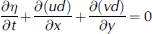
Solves for Sea Surface height. in the case of the embedded model or a fixed-depth oceanic boundary layer, we consider a boundary layer depth h _t demonstrated in figure 1a. for Simplicity, no drag is considered at the bottom of this boundary layer. ice velocity ui is related to the upper layer velocity by

Fig. 1.

Model Schematics of (a) a dynamically embedded ice–ocean model in an upper oceanic boundary layer (OBL) of fixed depth; (b) a levitated ice–ocean model on top of a fixed-depth OBL; and (c) a levitated Sea-ice model on top of barotropic ocean without an OBL.

(3)

Where h _i is Sea-ice thickness. Sea-ice and water density (ρ _i = 930 kgm^–3 and ρ _w = 1000 kgm^–3 respectively), the eulerian ice–water drag coefficient (c _w = 5.6×10^–4ms^–1) and the ice turning angle relative to water (= 25˚) remain constant. this is essentially the Slab boundary-layer approximation of Reference Heil and HiblerHeil and hibler (2002), whereby the ice velocity Scales with the integrated boundary-layer flow, but with

Different magnitude and direction. integrating the Same forcing over the upper layer as used for the vertically integrated equation, we obtain the velocity ut of the upper boundary layer:

(4)

While the embedding procedure used here is particularly Simple, it may be easily extended to ice–ocean models with multiple fixed or variable layers including baroclinic effects with Shear between the ice and other layers. the basic concept is that we provide a Simultaneous implicit Solution of the ice velocity, employing highly non-linear ice mechanics together with the barotropic mode of the ocean. for this purpose, ‘locking’ of the ice velocity to the integrated liquid ocean flow is a convenience adequate for this Study, but not essential to the general method.

In the case that levitated Sea ice (fig. 1b and c) is utilized, we Set Sea ice above the boundary layer to obey the equation

(5)

Where uo is the velocity of barotropic ocean as in figure 1c. in this version of the Stand-alone Sea-ice model, both the ice velocity in the drag term and the coriolis term are determined relative to the Surface velocity of the ocean. this is the form used in Some levitated models and leads to less extreme results than the case where the tilt term is taken to directly act on the ice, in which case only an ice velocity u_i would appear multiplied by the coriolis term as in the following equation:

(6)

For the levitated coupled ice–ocean model, we consider only a barotropic Slab ocean with no boundary layer So that the governing equations are (1), (2) and (5), with wind Stress and the ice interaction term in equation (1) replaced by the negative of the Second term in equation (5) So that the ocean model is being driven by the drag on the bottom of the ice cover. in the case of the embedded model, we consider an embedded boundary layer So the governing equations become (1–4).

In addition, we also examine an ice model driven only by Specified tides calculated with no modification of ice Stress into an ocean. this is done by utilizing equation (6) with Specified tides via the terms uo and this model, referred to as the ‘ice-only model’, is very close to the Reference Kowalik, Y.Proshutinsky, Johannessen, D.Muench and E.OverlandKowalik and proshutinsky (1994) formulation. this Standalone ice model is also the formulation of ice in coupled global ice–ocean levitated models (e.g. Reference Holland, Bitz, Hunke, H.Lipscomb and L.SchrammHolland and others, 2006) and will yield an ice response Similar to Such models if tides were added. this formulation, as is Shown below, induces very large artificial oscillations in the ice cover because the ice is levitated.

Since we are interested in a Solution of these equations in a form ultimately usable in ocean general circulation models, we utilized a variation of the Reference Dukowicz and D.SmithDukowicz and Smith (1994) implicit Solution whereby equations (1) and (2), the integrated free-surface ocean momentum equation and the conservation equation, are Simultaneously Solved implicitly. however, in the embedded case the Strong ice interaction necessitates an implicit Solution for the ice boundary layer (equation (4)). for Stability, this implicit ice Solution must be Solved together with the implicit ocean circulation. consequently, we Simultaneously Solve all of equations (1–4) (including an implicit Solution for half of the coriolis terms which were only treated explicitly by dukowicz and Smith) by a relaxation procedure for the ocean and ice (or equivalently upper boundary-layer equations). the relaxation procedure employed is directly analogous to the procedure used by Reference HiblerHibler (1979) to Solve the viscous–plastic Sea-ice dynamics equations. however, application of the procedure in this case requires the Solution of two vector equations at each relaxation node rather than only the ice vector equations as in Reference HiblerHibler (1979). all other aspects of the model are the Same as used in Reference Heil and HiblerHeil and hibler (2002).

3. Model Characteristics: Simulations and Observations

To examine the characteristics of the ice–ocean model, the effects of embedding and the relative roles of inertial and tidal forcing, three Sets of Simulations are carried out: one with tidal forcing alone, one with both wind and tidal forcing and one with only wind forcing. in all cases, we use ice mechanics with Spatially random Strengths but no temporal variation, Specified according to P* = 1.4[1.0 – 1.4(0.5 – R)]× 104nm^–1 for the random number 0 ≤ R ≤ 1. this random variation has proven more realistic for Simulating the initiation of linear kinematic features (Reference Hutchings, Heil and HiblerHutchings and others, 2005), as well as inertial variability that more closely approximates the heterogeneous character of the arctic ice cover than, Say, a constant Strength. we use an ice thickness extending to a depth of 3 m in the ocean: h_i=(3m)ρ _w/ρ _i.

For tidal forcing, amplitude vs time is Specified at the lower boundary of the grid (fig. 2). these data were taken from Simulation results covering a larger rectangular grid of which this grid is a Subset (essentially the Same as Reference Kowalik, Y.Proshutinsky, Johannessen, D.Muench and E.OverlandKowalik and proshutinsky, 1994). at high latitudes, direct gravitational forcing of tides is Small So that boundary forcing produces adequate tides for our mechanistic Study. the M2 tide has a period of 12.42 hours, Slightly Shorter than the inertial period of 12.46 hours on the constant f plane.

Our b-grid resolution of 42 km is about three times that of the finer Reference Kowalik, Y.Proshutinsky, Johannessen, D.Muench and E.OverlandKowalik and proshutinsky (1994) 14 km grid. while our course grid removes passages through the canadian arctic archipelago, comparisons with a higher-resolution b-grid tidal model Show that it produces Similar tides in the arctic basin with M2 forcing. a time-step of 202 S was used, Some five times longer than that of Reference Kowalik, Y.Proshutinsky, Johannessen, D.Muench and E.OverlandKowalik and proshutinsky (1994). our longer time-steps are allowable due to the implicit Solver, and are Short enough to negligibly damp tidal propagation. a von neumann boundary condition was applied at the open Southern boundary.

Linearly interpolated-in-time geostrophic winds beginning in october 2001 were derived from 6 hourly european centre for medium-range weather forecasts (ECMWF) reanalysis (era-40) mean Sea-level pressure fields Summarized in Reference Betts and BeljaarsBetts and beljaars (2003). the pressure fields were linearly interpolated, using the nearest-neighbor method, to the finer 14 km grid and then Spatially averaged to the 42 km grid. in the case of tides only, about 500 hours is adequate for a Steady tidal Solution. for cases including wind forcing, 3000 hours were run to provide adequate Statistics under different wind conditions for analysis of wind-induced Semi-diurnal variability. general but not direct comparisons were made in the wind+tidal Simulations to buoy-drift characteristics. central basin deformation characteristics from Reference Kwok, Cunningham and HiblerKwok and others (2003) were used for general Strain comparisons. the approximate locations of these comparisons are denoted by letters in figure 2. time Series from Simulated results were taken from gridcells a and b, the former over the deep ocean and the latter on the Siberian Shelf. the Reference Kwok, Cunningham and HiblerKwok and others (2003) deformation location near the pole at c was also used to compare our model output with their results. gridcell a tends to have central basin deep-water tidal characteristics, whereas b tends to have a Strong tidal regime with different rotational characteristics than the Reference Kwok, Cunningham and HiblerKwok and others (2003) deformation location c.

Fig. 2.

Land–sea mask used in numerical Simulations. Tidal forcing consists of variations in Sea Surface height along the lower boundary at ocean gridcells. Axis coordinates are Cartesian gridpoints. Spectral analysis is conducted for locations marked a–g.

3.1. Tide-only forcing: a comparison of embedded and levitated ice–ocean coupling

We compare the embedded and levitated models forced only with tidal forcing (no wind drag). the tidal amplitudes for the embedded and levitated models are Shown in figure 3a and b respectively. for comparison, the tidal amplitude of the barotropic model without Sea ice is Shown in figure 3c. amplitude is Similar for both embedded and levitated cases because ice cover has a relatively Small effect on tidal amplitude. the tides generally proceed anticlockwise around the basin, resulting in anticlockwise rotation of both ice and water parcel motion. the deformation inherent in the tidal forcing also typically has this character in the deep basin in terms of rotation of the Strain-rate ellipse (kwok and others, 2003). however, topography effects along, for example, the Siberian Shelf cause clockwise rotation of tides (shown below). a close examination of the tidal amplitude approaching the Siberian coast Shows that the levitated model Slightly amplifies the overall tidal amplitude in this region while reducing it Somewhat in the central basin. this relatively Small reduction is misleading Since the tidal velocity component is Substantially reduced in the levitated case along the Siberian coast.

Fig. 3.

Tidal amplitude in the absence of wind forcing for the Arctic basin portion of the grid for (a) the dynamically embedded model, (b) the levitated model and (c) the ice-free barotropic model.

For the embedded case, no drag at the base of the boundary layer and ocean bottom means that the embedded model yields identical tidal amplitudes where there is no ice interaction as would occur in an ice-free barotropic model. that this must be the case can be Seen from the governing equations Since the upper-layer equation is identical to the integrated layer except for ocean depth. by contrast, the levitated model has the unrealistic characteristic of producing both different tides and ice drift when there is no ice interaction.

Amplification and damping effects are much more clearly Seen in the tidal velocity characteristics (fig. 4) and ice velocity characteristics (fig. 5) Shown as rotary Spectra (Reference GonellaGonella, 1972) in deep-water central basin locations (figs 4a and 5a) and near Shore (figs 4b and 5b). for each rotary Spectrum presented, we use circles to denote anticlockwise rotation, and crosses to denote clockwise rotation in the direction of inertial oscillations. lefthand panels refer to the embedded model, and righthand panels present levitated model results.

Fig. 4.

Rotary Spectra (+ clockwise, о anticlockwise) for average ocean tidal velocities using tidal forcing only (no wind) for the embedded (left) and levitated (right) Sea-ice–ocean models at locations a (a) and b (b) in Figure 2. Note that relative power axes may be converted to power Spectral density by dividing by the frequency Separation between Spectral points.

Fig. 5.

(a, b) Rotary Spectra (+ clockwise, о anticlockwise) for average ice velocities using tidal forcing only (no wind) for the embedded (left) and levitated (right) Sea-ice models at locations a (a) and b (b) in Figure 2. (c) A comparison is Shown for the ‘ice-only’ levitated model Summarized in Equation (6) for locations a (left) and b (right).

The general character of the tides (and embedded ice in the free-drift limit) is Shown in figure 4 to be relatively Small and anticlockwise in the central basin and Substantially larger and clockwise nearer the Shores. in particular, the clockwise rotational peak is about two orders of magnitude higher than the anticlockwise peak near the coast and vice versa over deep water. this rotational feature is also present in the levitated model (fig. 4, righthand panels). however, for the levitated model, the tidal magnitude is reduced twofold in the nearshore region relative to the embedded case. the reverse effect, albeit Smaller, occurs in the central basin where the levitated model amplifies the clockwise tides by about 50%. analysis of the free-drift case of the levitated model Shows much of this effect is due to the mass of the ice (taken to be 3m in thickness here) and the resulting artificial inertial ice motion for the levitated case. in the free-drift limit with zero ice thickness, the levitated model yields identical tides to the embedded case, as must physically occur.

There are Significant differences in ice velocity between the two models. this is illustrated with the aid of rotary Spectra for the central basin (fig. 5a) and near Shore (fig. 5b). in the case of the central basin, the embedded model yields a dominant anticlockwise rotation consistent with the rotation direction of the tidal forcing noted above. however, in the case of the levitated model, there is effectively no consistent rotation in either direction. this means that the levitated model motion consists of oscillations along a Straight line at the Semi-diurnal peak. Such motion yields rotary Spectra with equal magnitude in both clockwise and counterclockwise directions, and is Symptomatic of a tendency in the levitated model to exaggerate clockwise motion in ice drift.

This tendency of the levitated model to exaggerate clockwise motion arises from the fact that the Stand-alone ice momentum equation (equation (5)) is a damped ‘rotary harmonic’ oscillator. it has a resonant frequency Shifted Slightly from the inertial period by the drag term. by ‘rotary harmonic’ we mean that the oscillator Selectively responds to rotational forcing parity with an enhanced clockwise reaction relative to the counterclockwise. the levitated central basin result is Somewhat modified by the ice interaction, but these essential features are Still present if we consider free drift (no ice interaction) with non-zero ice mass. in this case (not Shown), the embedded model yields identical tidal and boundary-layer drift results as would be obtained for a barotropic tidal model independent of ice thickness (evident in equations (1–3)). however, because of its unphysical nature, the levitated model yields Substantial and preferential clockwise motion amplification for the ice.

Note that the alternate Stand-alone Sea-ice model (fig. 5c), as presented in equation (6), amplifies the diurnal power in ice velocity in a relatively Similar manner to the primary levitated model. differences are due to different tides, as free-drift tides were used in the Stand-alone Sea-ice model, and to the fact that the Surface tidal currents are non-geostrophic, especially over deep water. the amplification of the clockwise rotary component is about a factor above the embedded case in the central basin (fig. 5c, left panel). over Shallow water the response is typically >1000 times the clockwise component for the embedded model, as Shown by the exceptional Shallow response in the right panel of figure 5c. this ‘ice-only model’ case demonstrates the artificial nature of forcing a Sea-ice model with ▽η from a Separate ocean model without providing necessary feedback to Sea Surface height and hence to ice divergence and convergence.

More generally it Shows that a coupled ice–ocean model must be used to obtain realistic ice tidal response.

We now turn attention to nearshore ice motion where Strong tidal effects occur (fig. 5b). here the embedded model ice mechanics modify the ice response to tidal forcing, whereas the levitated model not only modifies the ice response but also produces Spurious tidal currents (fig. 4b). in particular, the levitated ice response has a greatly enhanced amplification of the nearshore clockwise rotation, resulting in, we Suggest, an unrealistically large ice motion and related deformation. it is likely that the presence of this motion in the levitated Reference Kowalik, Y.Proshutinsky, Johannessen, D.Muench and E.OverlandKowalik and proshutinsky (1994) model contributed to their conclusions that high-frequency variability in ice production through deformation is Small in the central basin compared to nearshore regions. as in the central basin, the unphysical magnitude of the levitated result is buttressed by free-drift results for the levitated case where a Similar over-amplification is obtained. this contrasts with the embedded case, where tides are unchanged by the presence of ice in free drift and the ice response has a local clockwise motion reflecting the tidal boundary-layer forcing in this region.

The interesting anticlockwise rotation of the embedded ice velocities Shows how ice mechanics can cause ice to respond to the integrated tidal forcing coherent with the ocean (fig. 5b, lefthand panel). in particular, while the mainly anticlockwise forcing of arctic basin tides is Smaller than the opposite parity forcing on Some of the Shelves, the areal integral of this clockwise forcing is larger. hence the ice can move in a more coherent fashion, Smoothing out and reversing the vorticity of the ice motion expected from local tidal forcing. we note, however, that because of the lack of changes in the ice Strength due to deformation and advection, this effect may be over-amplified here.

3.2. Inertial- vs tide-driven drift and deformation

Of more relevance to the physics of ice-covered oceans is the combined role of tides and inertial variability in high-frequency Sea-ice drift and deformation. Reference Kwok, Cunningham and HiblerKwok and others (2003) included information on the rotational character of observed drift and deformation. here we present analogous rotational results of our embedded model output together with Selected levitated model results, and explicitly examine the contribution of tides and inertial variability to Sea-ice motion.

For an initial analysis of the tide–inertia interlink, we carry out combined wind- and tidally forced Simulations for the Several Simulated months described above. for comparison, a Second Simulation without tidal effects (wind only) was conducted for the Same time period. figure 6 Shows the ice-velocity results from these Simulations in the far- and nearshore regions, while figure 7 presents deformation for a central basin location near the Reference Kwok, Cunningham and HiblerKwok and others (2003) radarsat geophysical processor System (RGPS) measurement area. for observational perspective, figure 8 provides the rotary Spectra of hourly velocity from four arctic buoys whose positions are marked in figure 2 as letters: one on the Siberian Shelf (d), one Slightly off the Siberian Shelf (e), one near the pole (g) and one in the lincoln Sea near ellesmere island (f).

Fig. 6.

Rotary Spectra (+ clockwise, о anticlockwise) for modeled ice velocities in the embedded model for wind+tidal forcing and wind-only forcing at locations a (a) and b (b) in Figure 2. (c) Spectra for wind+tidal forcing for the levitated model in these two locations.

Fig. 7.

Rotary Spectra (+ clockwise, о anticlockwise) for a combination of Sea-ice deformation components at location c close to Reference Kwok, Cunningham and HiblerKwok and others’ (2003) observations in 2002 and 2003. (a) The embedded model with tidal forcing only; (b) the levitated model with tidal forcing; and (c, d) the embedded model using wind-only and wind+tidal forcing respectively.

Fig. 8.

Rotary Spectra (+ clockwise, о anticlockwise) for buoy velocity during February and March 2002. The buoys were in the locale of letters marked in Figure 2: (a) d (on the Siberian Shelf); (b) e (over deeper water adjacent to the Siberian Shelf); (c) g (central basin); and (d) f (Lincoln Sea).

To analyze the rotary character of the deformation rate in figure 7, we formed two time Series and 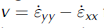from Sea-ice Strain-rate tensors. we used these to carry out a rotary Spectral analysis. the motivation for this was that for a System where the principal axes of Strain rotate uniformly with the ratio of the magnitude of the principal axes fixed, in the mohr’s circle construction (represented in a complex plane with real and imaginary components equal to u and v) the Strain-rate location uniformly rotates around the circle. it is therefore the exact analog to the rotation of the vector velocity of a particle moving in a circle. for more complex rotating Strain rates, this analogy breaks down, but nevertheless this method provides, in practice, a good estimate of the Sense of rotation of the Strain-rate tensor principal axes.

The main conclusion arising from the central basin Spectra in figures 6a and 5a is that the inclusion of wind forcing induces a Substantial clockwise inertial Signal that is amplified by the tides. moreover, this Signal is large enough to overwhelm the clockwise Signal arising from tidal forcing. this is not particularly Surprising given that the general amplitude of the clockwise oscillations is of order 20 m² S^–1 at the Semi-diurnal peak in both the wind and wind + tides case (fig. 6a). this can be compared to the much more pronounced peak in the tidal-forcing-only case (fig. 5a, lefthand panel) but nevertheless with a peak magnitude of about 10 m² S^–1 for the anticlockwise Spectra together with a much lower peak of about 0.5 m² S^–1 for the clockwise peak. in addition, in this central basin case the winds have transformed the Spectra to contain more red noise.

Overall, comparison of the wind + tides and wind-only cases (fig. 6a) Shows that adding wind and tidal forcing here creates a clockwise inertial peak 100 times greater than the original tides-only clockwise peak, and greater by at least a factor of two than the tidal anticlockwise peak. this peak is also Substantially greater than the wind-only inertial peak, indicating that it has been amplified by the tides. the best description of the central basin characteristics is that the inertial effects dominate, and are enhanced by, tidal forcing, and the overall rotation is clockwise. there is Still a tidal Signal there, but it is not Strong enough to dominate. this result is consistent with the Reference Kwok, Cunningham and HiblerKwok and others (2003) measurements, and the heil and Reference Hibler and M.SchulsonHibler (2002) inertial-only results. it is also generally consistent with observed buoy-drift Spectra in figure 8c.

However, this result is in Strong contrast to conclusions that could be drawn by adding wind forcing to the Reference Kowalik, Y.Proshutinsky, Johannessen, D.Muench and E.OverlandKowalik and proshutinsky (1994) model without a boundary layer: namely that the high-frequency variability in the central basin is dominated by tidal rather than inertial effects. how this conclusion could be reached is Shown in figure 6c, where the levitated model Spectra for wind + tides are Shown for the central basin and nearshore regions. in the case where wind forcing is added to the levitated model, there is very little addition of inertial power and/or amplification of clockwise rotation by the tides. hence, because of the artificial inertial resonance in the tidal forcing case alone (see fig. 5a), the central basin Signal is Still close to clockwise from tidal forcing alone.

In the case of the nearshore peak with embedding (fig. 6b), wind increases the clockwise inertial peak but in this location, even with Some tidal amplification in the wind + tides case, does not increase the Signal enough to overcome the tidal Signal with opposite parity. the tidal Signal is, for ice-mechanics reasons noted above, of opposite rotational parity to the local tides. in the case of the levitated model (fig. 6c), addition of winds produces much the Same result as tidal forcing only, with an excessive clockwise peak in the nearshore region.

It is unlikely that the wind-driven currents, effectively following f/d topography contours, account for any of the additional power in either the nearshore or central-basin locations. the maximum variance (not Shown) of the wind-driven currents occurs near the Siberian Shelf position, with a Semi-diurnal magnitude of about 10% of the tidal currents. these topography-following currents are driven by the average vorticity input enclosed by the contour (e.g. Reference Wang, Liu, Jin, Ikeda and J.SaucierPedlosky, 1986), or alternatively by green’s theorem: the line integral of the Surface ‘stress’ vector into the ocean (wind Stress minus ice force) tangent to the topography contour integrated around the closed contour. because of the complexity of these barotropic currents, the Sense of the ice rotation induced is difficult to access a priori. we also note in general that our barotropic currents and hence Sea Surface height are in Strong contrast to proshutinsky and johnson (1997) who effectively used a flat-bottom ocean with minimal bottom torque effects So that the wind-driven circulation largely Simply follows the wind direction and can (unrealistically) effectively reverse almost immediately.

The lack of a dominant clockwise rotation in Simulated Siberian-shelf ice velocity is consistent with observed buoy drift Shown in figure 8. the Siberian-shelf buoy of figure 8a and to a lesser degree figure 8b lacks dominance by the clockwise Semi-diurnal peak. the buoy-drift record Shows what appear to be very Strong oscillations with a weak Semi-diurnal peak and Some preference toward clockwise rotation.

The lincoln Sea buoy Spectra (fig. 8c) are in contrast to the Siberian Shelf buoy (fig. 8a). at first glance, the lincoln Sea time Series has a Similar character to that of the Siberian Shelf. however, it also Shows a Strong inertial-oriented peak, consistent with the Reference Kwok, Cunningham and HiblerKwok and others (2003) observations and central-basin model results. the power here is notable because it is an area of Strong ice conditions. this Suggests that the Substantial ice-thickness variations in the region may have more of an inertial or tidal origin than previously thought. the ice build-up here has previously been attributed to land–sea boundary effects. the buoy in the central basin (fig. 8b) Shows only a weak tidal inertial peak, Suggesting that the Strong peak in the Reference Kwok, Cunningham and HiblerKwok and others (2003) observations may have Some relationship to the topography variations of the lomonosov ridge.

The central-basin deformation Spectra Shown in figure 7 generally Support the idea of Superposition of inertial variability onto the tidal Signal. but an important addition to this notion is that the deformation Signal has a broader and more Substantial region of inertial-oriented power. this result is generally in agreement with observational results (e.g. Reference Hibler, Weeks, Kovacs and F.AckleyHibler and others, 1974; Reference Kwok, Cunningham and HiblerKwok and others, 2003), Showing that even in the absence of a Strong inertial Signal under compact ice conditions, there can be a deformational Signal. what is new here is that this Strain rate tends to rotate in terms of the principal axes rotating, and this rotational Sense is dominated by the inertial direction in the central basin. a Strong point of these model calculations is that they correctly Simulate this deformation feature, even with temporally constant ice Strengths.

With tidal forcing only (fig. 7a and b), the results Show a deformation in the central basin rotating in the opposite Sense to that observed in the embedded case, providing more Support for the dominance of inertial power there (as Suggested by Reference Heil and HiblerHeil and hibler, 2002). for the levitated model, the artificial inertial resonance yields a clockwise rotating Strain rate for tidal forcing only, Suggesting that the tidal Signal dominance (suggested by Reference Kowalik, Y.Proshutinsky, Johannessen, D.Muench and E.OverlandKowalik and proshutinsky, 1994) is as in the case of ice velocity, likely the right answer for rotation direction and for the wrong reason: i.e. it is likely a model artefact, being directly due to tidal forcing on a levitated ice model with an artificial resonance. in the embedded case, the tidal forcing plays a role, but only via amplifying inertial clockwise Strain-rate rotation induced by the wind.

4. Discussion and Conclusions

The results of our Simulations Suggest there are Substantial erroneous features inherent in levitated Sea-ice models. this Seems to be true even in our Seemingly Safe case of Sea ice coupled to a Single-layer barotropic ocean. the worst effects of this coupling can be avoided by Slightly degrading this coupling by parameterizing the ocean tilt term on the pack ice to be a coriolis term proportional to the ocean Surface velocity. but even Still, the coupling in the arctic generally leads to excessive tidally induced ice velocities on the Siberian Shelf and a reduction of tides in that region. moreover, in the central basin the levitated coupling leads to excessive clockwise motion in the absence of ice interaction or wind, even though the tidal forcing is locally counterclockwise.

Both these deleterious effects can largely be traced to the fact that the levitated ice cover, even with Some drag, is a resonant damped harmonic oscillator with parity-dependent response. this leads to a parity-dependent artificial resonance when levitated ice is employed. because of this preferential response to clockwise forcing and the fact that ice convergence and divergence is not considered in ocean volume conservation, the levitated model dramatically over-amplifies response in that direction. by application of newton’s third law in the nearshore region, this effect leads to a bogus damping of the amplitude of the tidal velocities. the embedded model together with the combined implicit Solver used here has no Such unrealistic results and reduces to the free barotropic tide Solution in the case of no ice interaction even with finite ice mass and a boundary layer. the levitated model has an artificial inertial resonance, whereas the embedded model does not.

Probably the most important new physical idea arising from this Study is that, even in Strong tidal regions, ice mechanics can cause the rotational response of the ice motion to change Sign in Spite of very Strong local forcing. in the arctic, this response is counter-intuitive at first glance Since it effectively means that a Strong tidal forcing can be overcome by a much Smaller one. however, the Smaller forcing covers a larger region, and Since Sea ice is a good integrator the integral over the larger region dominates. while we have only represented Semi-diurnal tides here, this notion can be extended to multispectral tides and could be a candidate theory to explain the presence of multiple peaks in antarctic ice Signals in Strong ice conditions (demonstrated by Reference Geiger, Hibler and F.AckleyGeiger and others, 1998).

Apart from this important integrating notion, the various combinations of wind-driven and tidal Simulations analyzed here Support the tidal amplification concept of inertial and tidal motion. under this mechanism, increased inertial forcing from wind or ice-mechanics effects raises the clockwise rotary character of power which may then be amplified by the clockwise rotary component of the tidal forcing. hence the tidal amplification plays a role, but only through the intermediary of inertial power induced by the wind. tidal forcing alone tends to yield the incorrect rotation direction for Sea-ice velocity and Strain-rate rotation in the central basin. in the nearshore region, this Same effect applies but the Spatially integrating Sea-ice effect is Substantial, and during certain periods non-local tidal effects can return to modulate at least the amplitude of the inertial Signal, if not the direction and phase. we note, however, that our Simulations are limited by a lack of temporal ice-strength evolution through ice advection, deformation, growth and melt. inclusion of these features is in progress. it is possible that these features may lead to Sporadic periods when the Spatial-average response becomes much weaker or Stronger.