1. Introduction
Supercritical pressure (SCP) fluids are encountered in many practical applications, including liquid rocket engines (Yang Reference Yang2000; Wang et al. Reference Wang, Zhang, Li, Yeh and Yang2018) regenerative cooling (Xie et al. Reference Xie, Xu, Lei, Li, Li and Sunden2022), thermal power cycles (White et al. Reference White, Bianchi, Chai, Tassou and Sayma2021) and novel nuclear reactors. In these processes, the SCP fluids often undergo a transcritical change of temperature, characterised by significant variations in thermophysical properties, known as the pseudo-boiling phenomenon. As illustrated in figure 1, the thermophysical properties of SCP
 $\mathrm {CO}_{2}$
(critical point is at 304.25 K, 7.383 MPa) at 8 MPa exhibit abrupt and nonlinear variations within a narrow range around pseudo-boiling temperature
 $T_{\textit {pb}}$
(defined as the temperature at which the isobaric specific heat capacity reaches its maximum value, here
 $T_{\textit {pb}}=307.8\,\text {K}$
). Such property variation behaviour deviates substantially from the perfect fluid assumption, and is referred to here as the real-fluid effect of SCP fluids (Ding et al. Reference Ding, Li, Wang, Ni and Wang2024). The real-fluid effect, particularly the density variation embedded with the momentum and energy transport, results in complex turbulent dynamics and poses the challenges to existing turbulence models that are based on ideal-gas conditions. Therefore, understanding the underlying mechanisms of how density fluctuations influence small-scale turbulence motions and heat transfer is essential for the accurate modelling and simulation of SCP fluid flows. To this end, the present study investigates systematically the turbulence statistics of heated and cooled turbulent wall-bounded channel flows at SCP, with emphasis on the detailed real-fluid effects imposed by abrupt property variations.
Numerous experimental studies have been conducted to explore global heat transfer characteristics of SCP fluids. Huang et al. (Reference Huang, Coleman and Bradshaw2016) reviewed convection heat transfer experiments with SCP fluids in strongly heated or cooled pipes. The effects of various parameters, such as inlet temperature, pressure and mass flow rate, pipe diameter, and wall heat flux on heat transfer were examined. Several research groups (Wang et al. Reference Wang, Zhang, Li, Yeh and Yang2018; Guo et al. Reference Guo, Xiang, Zhang, Huai, Cheng and Cui2019; Xie et al. Reference Xie, Liu, Yan, Xie and Boetcher2020; Zhang et al. Reference Zhang, Xu, Liu, Li, Wu and Dang2022; Jin et al. Reference Jin, Zhao, Wan, Chen, Liu, Wang, Li and Wan2023) paid special attention to the occurrence of heat transfer deterioration (HTD) and to the development of predictive heat transfer correlations and buoyancy criteria. Their studies showed that HTD may result from variations in thermophysical properties, as well as buoyancy and flow acceleration. Heat transfer correlations generally adopt the form of the Dittus–Boelter correlation (Dittus Reference Dittus1929), with additional terms to account for these variations. While most of these correlations provide reasonable predictions for heat transfer coefficients in both normal and enhanced heat transfer regimes, they fall short in accurately predicting HTD. Wang et al. (Reference Wang, Zhang, Li, Yeh and Yang2018) attributed these issues to the lack of detailed measurements in flow velocity and turbulence at SCP. Unfortunately, comprehensive turbulence statistics of SCP fluids from experiments remain difficult due to the challenges of experimental diagnostics posed by severe operating conditions (Yoo Reference Yoo2013). As such, a detailed assessment of the effects of large density variation, as well as its fluctuating behaviour in turbulent wall-bounded flows, remains an open subject. An alternative and effective approach to explore the flow physics and detailed turbulence statistics is through direct numerical simulations (DNS).
Thermodynamic properties of
 $\mathrm {CO}_{2}$
at pressure 8 MPa: (a) density
 $\rho$
and isobaric specific heat capacity
 $c_{p}$
; (b) thermal conductivity
 $\lambda$
and dynamic viscosity
 $\mu$
.

In DNS studies of variable density flows at atmospheric pressure, the effect of density fluctuation on turbulence is typically neglected because of the relatively low amplitude with respect to the mean density. This appears valid based on the Morkovin assumption (Morkovin Reference Morkovin1962; Bradshaw Reference Bradshaw1977) that only mean density variation is important in turbulence dynamics if the root mean square (r.m.s.) of density fluctuation is small enough (less than 10 % of the local density). Nevertheless, the influence of density fluctuations on near-wall turbulence has been found to be substantial in several studies. You, Yoo & Choi (Reference You, Yoo and Choi2003) and Bae, Yoo & Choi (Reference Bae, Yoo and Choi2006) performed DNS of strongly heated internal air flows, and found that density fluctuation, accounting for 10 % of the local mean density, has a negligible influence on turbulence structure. However, the buoyancy production term, arising from the correlation between density and velocity fluctuations, is significant, and it reduces overall production of turbulent kinetic energy (TKE). Chu, Laurien & McEligot (Reference Chu, Laurien and McEligot2016) and Zhao et al. (Reference Zhao, Liu, Ge, Li, Zhao and Wan2018) further confirmed that the buoyancy production exerts a negative effect on TKE in strongly heated upward air flows. In fully developed channel flows, Patel et al. (Reference Patel, Peeters, Boersma and Pecnik2015, Reference Patel, Boersma and Pecnik2016) employed DNS to examine the influence of temperature-dependent density and viscosity. They found that for moderate density and viscosity gradients where property fluctuations are minor (approximately 13 % of the mean value), Morkovin’s hypothesis holds for second-order statistics, but fails for the higher-order moments of velocity fluctuations. Additionally, Ng et al. (Reference Ng, Ooi, Lohse and Chung2015, Reference Ng, Ooi, Lohse and Chung2018) studied vertical natural convection in a channel at varying Rayleigh numbers. Their results indicated that density fluctuations were dynamically significant through large buoyancy forces, leading to the emergence of a bi-directional wind. The above studies have indicated that large-amplitude density fluctuation could pose a significant effect on turbulence statistics, and the underlying mechanism needs to be addressed.
In SCP flows, the fluid density can vary dramatically and nonlinearly over a small temperature range near
 $T_{\textit {pb}}$
(see figure 1). The real-fluid effect is stronger and more complex than its subcritical counterpart (Liu, Wang & Yang Reference Liu, Wang and Yang2021). Several researchers (Bae, Yoo & Choi Reference Bae, Yoo and Choi2005; Nemati et al. Reference Nemati, Patel, Boersma and Pecnik2016a
,Reference Nemati, Patel, Boersma and Pecnik
b
; Pandey, Chu & Laurien Reference Pandey, Chu and Laurien2017; Cao et al. Reference Cao, Xu, Yan, He and Jiang2021; Zhao et al. Reference Zhao, Wan, Jin, Chen, Li and Peng2021) have performed DNS analysis on the in-tube heating or cooling of fluid flows at various SCPs, focusing on the mechanisms of buoyancy or thermal acceleration effect induced by density variation on turbulence modulation. Some of these findings include the following. (i) The density of SCP fluids evaluated at the mean temperature (or enthalpy) does not always match their corresponding Reynolds- or Favre-averaged mean value, especially near
 $T_{\textit {pb}}$
, caused by the large density fluctuations and the nonlinear dependence on enthalpy. (ii) Compared to ideal-gas problems, additional terms related to density fluctuations in the turbulent mean equations could partially offset the increase or decrease in TKE and significantly affect the heat transfer by modifying turbulent heat flux. (iii) The insufficient consideration of density fluctuation effect (or buoyancy production term) in the treatment of the streamwise turbulent heat flux could lead to the failure of turbulence models to capture the characteristic sharp peak of the wall temperature in SCP fluid flows. The effects of buoyancy and thermal acceleration can be regarded as the indirect effect of variable density on heat transfer by mitigating the flow field. The direct impacts of property variations, on the other hand, are much less explored.
Peeters et al. (Reference Peeters, Pecnik, Rohde, Van Der Hagen and Boersma2016) investigated turbulent flow and heat transfer in an SCP
 $\mathrm {CO}_{2}$
annular pipe with two isothermal walls of a temperature difference of 20 K. They found that the augmented fluctuations of density and dynamic viscosity influence the streak evolution and contribute to the decreased turbulence intensity near the heated wall at SCP. Similarly, Kim, Hickey & Scalo (Reference Kim, Hickey and Scalo2019) explored the SCP turbulent heat transfer of R-134a in a fully developed channel flow with isothermal wall temperature differences of 5 K, 10 K and 20 K, highlighting intense thermodynamic fluctuations in the pseudo-critical region near the heated wall, in conjunction with reduced turbulence intensity. This attenuation of turbulence is attributed to the impoverishment of the turbulent flow structures near the pseudo-boiling point due to density ejections. Wan et al. (Reference Wan, Zhao, Liu, Wang and Lei2020) examined the effect of density fluctuation on the velocity and temperature scaling laws in the near-wall boundary layer of SCP
 $\mathrm {CO}_{2}$
at wall temperature differences ranging from 5 K to 25 K. They demonstrated the feasibility of semi-local scaling laws based on the Trettel and Larsson velocity transformation under small density fluctuation. Furthermore, they improved the temperature scaling law by considering the effect of large specific heat variations. The aforementioned studies, however, are limited to small wall temperature differences associated with minor density fluctuations (approximately less than 15 % of the local density). The study of large-amplitude density fluctuation effects induced by big wall temperature differences is much less documented.
Kawai (Reference Kawai2019) performed DNS of fully developed parahydrogen turbulent boundary layers on a flat plate under heated transcritical and unheated non-transcritical conditions. The density fluctuation in the vicinity of the heated wall exceeds 40 % of the mean value, and significantly impacts the TKE budgets by contributing to additional turbulent mass flux. Ma, Yang & Ihme (Reference Ma, Yang and Ihme2018) considered transcritical channel flows of nitrogen with wall temperature difference 200 K using DNS. They found that the semi-local scaling law near the heated wall shows poor performance owing to the intensified density fluctuation. Li, Pei & Bai (Reference Li, Pei and Bai2022) further explained such issues by attenuated near-wall streamwise coherence at high-amplitude density fluctuation near the heated wall. Despite these studies, the understanding of interplay between variable density and turbulence statistics at SCP remains limited and requires further investigation.
In this study, we intend to investigate the real-fluid effect imposed by various amplitudes of density fluctuations on turbulence statistics in fully developed turbulent channel flows. The different degrees of density variation are achieved in the wall-normal direction by varying channel wall temperatures at a given SCP. The present work distinguishes itself in two significant aspects compared to previous studies. First, the amplitudes of density fluctuations considered here are wider (up to 55 % of the local mean value) than those in most documented literature, enabling a more comprehensive analysis of density-perturbed turbulence characteristics. Second, the intricate mechanisms by which density fluctuation modifies TKE transport and turbulent heat transfer are explored systematically. The paper is organised as follows. Section 2 provides a detailed description of the theoretical formulation and problem set-up. Section 3 presents the results and discussions. Finally, § 4 concludes with the key insights from this study.
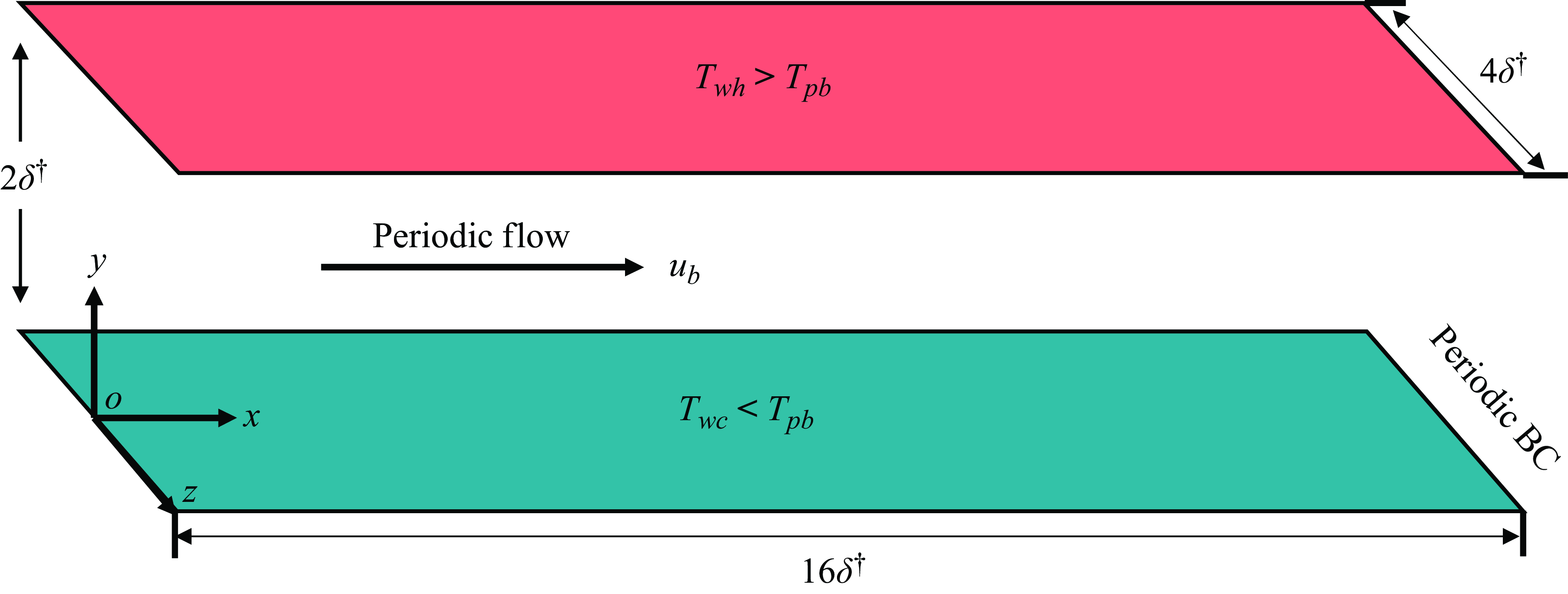
Schematic diagram of flow region and boundary conditions.

2. Theoretical formulation
2.1. Conservation equations
In the context of a low-speed channel flow involving a single-component fluid, the variation of thermophysical properties results mainly from a heat transfer process induced by temperature difference between the upper and lower walls (see figure 2). We adopt the low Mach number assumption, and focus mainly on scenarios where the changes in thermophysical properties due to acoustic effects and pressure alterations are disregarded, that is, the heat transfer process is treated as a thermodynamically constant-pressure process (Bae et al. Reference Bae, Yoo and Choi2005). The thermophysical properties of SCP fluids, such as density and dynamic viscosity, are considered solely dependent on temperature. The low Mach number governing equations for a fully developed channel flow driven by a mean streamwise pressure gradient without the effect of buoyancy can be expressed in tensor form as follows: mass,
 \begin{equation} \frac {\partial \rho }{\partial t} + \frac {\partial (\rho u_i)}{\partial x_i} = 0, \end{equation}
momentum,
 \begin{equation} \frac {\partial \rho u_i}{\partial t} + \frac {\partial }{\partial x_j} ( \rho u_i u_j + p \delta _{ij} - \tau _{ij} ) - \delta _{1i} f_i = 0, \end{equation}
energy,
 \begin{equation} \frac {\partial h}{\partial t} + \frac {\partial }{\partial x_i} \left ( \rho u_i h + q_i \right ) = 0, \end{equation}
where
 \begin{align} \tau _{ij} = \frac {\mu }{Re} \left ( \frac {\partial u_i}{\partial x_j} + \frac {\partial u_j}{\partial x_i} - \frac {2}{3} \delta _{ij} \frac {\partial u_k}{\partial x_k} \right ), \end{align}
 \begin{align} q_i = -\frac {\lambda }{Re_0\, Pr_0}\, \frac {\partial T}{\partial x_i} = -\frac {1}{Re_0\, Pr_0}\, \alpha\, \frac {\partial h}{\partial x_i}, \quad \alpha = \frac {\lambda }{c_p}.\end{align}
All variables in the above equations are dimensionless and are defined as follows:
 \begin{align} x_i &= \frac {x_i^\dagger }{\delta ^\dagger },\quad u = \frac {u^\dagger }{u_b^\dagger },\quad v = \frac {v^\dagger }{u_b^\dagger },\quad w = \frac {w^\dagger }{u_b^\dagger },\quad t = \frac {t^\dagger u_b^\dagger }{\delta ^\dagger },\quad p = \frac {p^\dagger }{\rho _{pb}^\dagger (u_b^\dagger )^2}, \end{align}
 \begin{align} \rho &= \frac {\rho ^\dagger }{\rho _{pb}^\dagger },\quad \mu = \frac {\mu ^\dagger }{\mu _{pb}^\dagger },\quad \lambda = \frac {\lambda ^\dagger }{\lambda _{pb}^\dagger },\quad c_p = \frac {c_p^\dagger\, \unicode{x0394} T^\dagger }{\unicode{x0394} h^\dagger }, \quad T = \frac {T^\dagger - T_{wc}^\dagger }{\unicode{x0394} T^\dagger }, \end{align}
 \begin{align} \quad h &= \frac {h^\dagger - h_{wc}^\dagger }{\unicode{x0394} h^\dagger },\quad Re_0 =\frac {\rho _{pb}^+ u_b^\dagger \delta ^\dagger }{\mu _{pb}^\dagger },\quad Pr_0 = \frac {\mu _{pb}^\dagger c_p^\dagger\, \unicode{x0394} h^\dagger }{\lambda _{pb}^\dagger\, \unicode{x0394} T^\dagger }. \end{align}
The superscript
 $\dagger$
denotes a dimensional value; the subscript ‘pb’ represents the value of the thermophysical property at the pseudo-boiling temperature. Additionally, the subscripts ‘wc’ and ‘wh’ define the parameters at the cooled and heated walls, respectively. Here,
 $\delta ^\dagger$
is the half-width of the channel, and
 $u_b^\dagger$
is the bulk velocity;
 $\unicode{x0394} T^\dagger$
and
 $\unicode{x0394} h^\dagger$
denote the temperature and enthalpy differences between the heated and cooled walls, respectively. The characteristic Reynolds number
 $ Re_0$
is based on
 $u_b^\dagger$
and
 $\delta ^\dagger$
;
 $ {Pr}_0$
is the reference Prandtl number based on a ratio of
 $\unicode{x0394} h^\dagger$
and
 $\unicode{x0394} T^\dagger$
. Additionally,
 $ f_i$
is a body force term in the momentum equation, which represents the
 $ i$
th component of the body force vector. This body force serves as a streamwise-homogeneous substitute for the pressure gradient, providing the necessary momentum driving force.
2.2. Computational set-up and numerical method
Figure 2 shows a schematic of the computational configuration for the turbulent channel flow in the present study. The channel dimensions are defined as
 $x^\dagger = 16 \delta ^\dagger$
in the streamwise direction,
 $y^\dagger = 2 \delta ^\dagger$
in the wall-normal direction, and
 $z^\dagger = 4 \delta ^\dagger$
in the spanwise direction. The working fluid is CO
 $_2$
, and the operating pressure
 $P^\dagger$
is
 $8 \text { MPa}$
. Both the upper and lower walls of the channel serve as isothermal boundaries. The temperature of the cooled wall (lower wall,
 $y= 0$
) is maintained below the pseudo-boiling temperature (i.e.
 $T_{\textit {pb}}^\dagger = 307.8 \text { K}$
at
 $8 \text { MPa}$
), while the temperature of the heated wall (upper wall,
 $y = 2$
) exceeds
 $T_{\textit {pb}}^\dagger$
. Such a set-up ensures that CO
 $_2$
in the channel undergoes the pseudo-boiling process. The temperatures of the heated and cooled walls, along with
 $T_{\textit {pb}}^\dagger$
, adhere to the relationship
 $T_{\textit {wh}}^\dagger - T_{\textit {pb}}^\dagger = T_{\textit {pb}}^\dagger - T_{\textit {wc}}^\dagger$
, which facilitates the direct comparison of turbulence characteristics between the heated and cooled wall sides with different levels of density variations. Both walls are treated as no-slip. The boundaries in the streamwise and spanwise directions are set as periodic, with the momentum transport driven by the volume-averaged pressure gradient, and the enthalpy transport driven by the temperature difference between the channel walls.
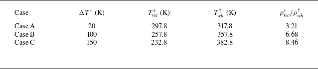
To explore the effect of density fluctuation on the turbulence statistics in the wall-bounded channel flow, three cases, hereinafter referred to as SCP cases, with varying temperature differences (
 $\unicode{x0394} T^\dagger$
) between heated and cooled walls, are considered (
 $\unicode{x0394} T^\dagger = 20$
,
 $100$
and
 $150 \text { K}$
). Increasing wall temperature difference leads to the elevation of density ratio between the lower and upper walls, as listed in table 1. As will be shown later, a higher density ratio between the walls generates larger density variation in the wall-normal direction, which has a profound impact on turbulence statistics in wall-bounded flows. During the simulations, the bulk Reynolds number for all cases is fixed at
 $ \textit {Re}_b = 5705$
according to the channel height
 $2\delta ^\dagger$
.
Wall temperature and associated physical parameter settings:
 $\unicode{x0394} T^\dagger$
(temperature difference),
 $T_{\textit {wc}}^\dagger$
(cooled wall temperature),
 $T_{\textit {wh}}^\dagger$
(heated wall temperature) and
 $\rho _{{wc}}^\dagger / \rho _{{wh}}^\dagger$
(density ratio of cooled and heated walls).

The numerical scheme employs a kinetic energy-conservative space–time discretisation scheme (Pierce & Moin Reference Pierce and Moin2004), combined with fourth-order central difference, adaptive Courant–Friedrichs–Lewy (CFL) time-stepping, and a semi-implicit iteration scheme (Wall, Pierce & Moin Reference Wall, Pierce and Moin2002). To address oscillations resulting from excessive enthalpy gradients, the fifth-order WENO scheme is implemented. Thermophysical properties, including density, are updated from a property table based on enthalpy and constant thermodynamic pressure (8 MPa), as
 $ \rho = \rho (P, h)$
. This table is derived from the pre-established NIST REFPROP database (Lemmon, Huber & McLinden Reference Lemmon, Huber and McLinden2010). Validation of the present DNS methodology is provided in Appendix B.
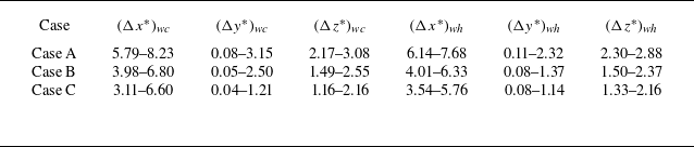
Summary of mesh sizes with respect to the semi-local viscous length scale near the cooled wall and the heated wall, where
 $\unicode{x0394} x^*$
,
 $\unicode{x0394} y^*$
,
 $\unicode{x0394} z^*$
are grid resolutions in semi-local units.

2.3. Grid resolution
The computational grid system utilised in all cases consists of
 $N_x \times N_y \times N_z = 384 \times 256 \times 256$
, where
 $N_x$
,
 $N_y$
and
 $N_z$
represent the total number of grids in the streamwise (
 $x$
), wall-normal (
 $y$
) and spanwise (
 $z$
) directions, respectively. The streamwise and spanwise directions employ uniformly spaced grids, while the wall-normal direction employs a stretched grid distribution of a hyperbolic tangent function to adopt significant gradients of physical quantities. Table 2 presents the grid resolution in different directions characterised by the semi-local viscous length
 $\delta _v^*$
(Huang et al. Reference Huang, Coleman and Bradshaw1995) at the cooled and heated walls, with
 \begin{align} \unicode{x0394} x_{i,\textit {wc}}^* = \frac {\unicode{x0394} x_i}{\bar {\delta }_{v,\textit {wc}}^*},\quad \bar {\delta }_{v,\textit {wc}}^* = \frac {\bar {\mu }}{\bar {\rho } \, \bar {u}_{\tau ,\textit {wc}}^*},\quad \bar {u}_{\tau ,\textit {wc}}^* = \sqrt {\frac {\bar {\tau }_{\textit {wc}}}{\bar {\rho }}},\end{align}
 \begin{align} \unicode{x0394} x_{i,\textit {wh}}^* = \frac {\unicode{x0394} x_i}{\bar {\delta }_{v,\textit {wh}}^*},\quad \bar {\delta }_{v,\textit {wh}}^* = \frac {\bar {\mu }}{\bar {\rho } \, \bar {u}_{\tau ,\textit {wh}}^*},\quad \bar {u}_{\tau ,\textit {wh}}^* = \sqrt {\frac {\bar {\tau }_{\textit {wh}}}{\bar {\rho }}},\end{align}
 \begin{align} \unicode{x0394} x_i = \unicode{x0394} x,\quad \unicode{x0394} y,\quad \unicode{x0394} z.\end{align}
Based on the scaled mesh sizes in three directions shown in table 2, it is believed that the grid scales meet the wall resolution requirements (Kim et al. Reference Kim, Hickey and Scalo2019). Further validation is performed to examine whether the grid resolution meets the Kolmogorov dissipation scale
 $\eta _v$
required for momentum transport, and the Batchelor scale
 $\eta _\theta$
required for scalar transport. Figure 3 illustrates the resolution distribution in the streamwise, wall-normal and spanwise directions in all SCP cases. Here,
 \begin{equation} \eta _v \equiv \left ( {\bar {\nu }^3}/{\bar {\epsilon }} \right )^{0.25}, \quad \eta _\theta \equiv {\eta _v}/{\sqrt {\overline {\textit {Pr}}}}. \end{equation}
It is found that the grid spacings in the
 $x$
,
 $y$
and
 $z$
directions adhere to
 \begin{align} \unicode{x0394} x = (1.83 {-} 4.55) \eta _v = (2.41 {-} 7.95) \eta _\theta , \end{align}
 \begin{align} \unicode{x0394} y = (0.03 {-} 0.94) \eta _v = (0.5 {-} 1.63) \eta _\theta , \end{align}
 \begin{align} \unicode{x0394} z = (0.68 {-} 1.71) \eta _v = (0.91 {-} 2.98) \eta _\theta , \end{align}
which ensures that the present grid resolution adequately captures all relevant scales.
3. Results and discussions
Our aim is to investigate the effects of varying density fluctuations in SCP
 $\mathrm {CO}_{2}$
on the wall-bounded turbulent flow and heat transfer. First, we will analyse the variations in density both qualitatively and quantitatively. Then we will examine the relative contributions of density fluctuation to turbulence statistics, including first-order and second-order moments. Next, we will explore the mechanisms by which density fluctuation impacts turbulence statistics in the momentum and energy transports, in terms of TKE, turbulent shear stress and turbulent heat flux. These analyses are facilitated by the analytical methods of statistical decomposition, budget analysis and quadrant analysis. Then the effects of density fluctuations are further assessed through the skin-friction coefficient and Nusselt number, as the observed physics of turbulence and heat transfer eventually manifest in these quantities. Finally, we will investigate the effects of density fluctuation on the instantaneous flow structures to provide additional insights. Before proceeding with the analysis and discussion, the notation is explained briefly: the Reynolds-averaged and fluctuation components of a physical quantity
 $\varphi$
are denoted as
 $\bar {\varphi }$
and
 $\varphi '$
, respectively, while the Favre-averaged and fluctuation components are denoted as
 $\tilde {\varphi }$
and
 $\varphi ''$
, respectively.
Scale analysis: (a) Kolmogorov scale and (b) Batchelor scale for x, y and z directions. Solid line indicates case A, dashed line indicates case B, dotted line indicates case C. Black indicates streamwise direction, red indicates wall-normal direction, blue indicates spanwise direction.

Instantaneous cross-sectional views (
 $y{-}z$
plane) of (a–c) density and (d–f) Prandtl number (
 $\textit {Pr}$
) in (a,d) case A, (b,e) case B, and (c,f) case C, at
 $x = 8$
. The black line in each plot represents the temperature contour of
 $T_{\textit {pb}}$
, the pseudo-boiling point

3.1. Mean property variations
Since all simulated cases have both heated and cooled walls, the fluid is of high density near the cooled wall and of low density near the heated wall. Figures 4(a–c) show instantaneous values of density in cases A, B and C, respectively. Near the wall, the mixing between high-density fluid and low-density fluid is enhanced by turbulent motions. Furthermore, a clear interface of density change in the vicinity of the heated wall can be seen in case C, indicating a substantially large density gradient. The corresponding distributions of Prandtl number (
 $\textit {Pr}$
) are presented in figures 4(d–f). It is found that the maximum value of
 $\textit {Pr}$
, corresponding to the pseudo-boiling point (black contour line), is observed very close to the heated wall in all cases.
Figure 5 depicts the wall-normal profiles of normalised mean temperature and enthalpy in all cases. The pseudo-boiling point shifts towards the heated wall with increasing wall temperature difference, resulting in increasingly sharp gradients in temperature and enthalpy near the heated wall. This trend significantly impacts the density profile. Figure 6(a) illustrates the wall-normal distributions of the mean density. Significant mean density variation is observed near the heated wall in all cases. In particular, in case C with the largest temperature difference (
 $\unicode{x0394} T = 150\ \text {K}$
), the density near the heated wall (
 $y\in [1.75, 2.0]$
) decreases by approximately 5.8 times. Figure 6(b) shows the wall-normal profiles of the r.m.s. density fluctuation
 $\rho '_{\textit {rms}}$
relative to the local mean values of density
 $\bar {\rho }$
in all cases, where
 $\rho '_{\textit {rms}} = \sqrt {\overline {\rho ^2} - \bar {\rho }^2}$
. The r.m.s. fluctuations are much stronger near the heated wall than those near the cooled wall. This could be attributed to the fact that stronger mean property variations occur near the heated wall where the pseudo-critical point exists. In cases B and C with large mean density variation,
 $\rho '_{\textit {rms}}$
reaches 45 % to 55 % of the mean density near the heated wall. Such a level of density fluctuation renders Morkovin’s hypothesis invalid, i.e. the large amplitude of density fluctuation could exert a substantial influence on turbulence statistics. It determines the relative differences between Favre- and Reynolds-averaged statistics, resulting in discrepancies of approximately 12 % for the first-order moments, and approximately 30 % for the second-order moments (see Appendix A). To obtain deeper insight, the mechanisms underlying the interactions between density fluctuation and turbulence statistics are explored systematically in the following subsections. For demonstration, we will choose three typical turbulence statistics involved in the transport of momentum and energy in fully developed channel flows: TKE, turbulent shear stress and turbulent heat flux. They represent the salient characteristics of turbulent flows and heat transfer, and are also important for turbulence modelling in SCP fluid flows.
Distributions of normalised mean (a) temperature, and (b) enthalpy. Black solid line indicates case A, red dashed line indicates case B, blue dotted line indicates case C.

Distributions of (a) normalised mean density, and (b) r.m.s. fluctuation of density. Black solid line indicates case A, red dashed line indicates case B, blue dotted line indicates case C.

3.2. Effect of density fluctuation on TKE transport
The effect of density fluctuation on TKE transport is explored first. The TKE, defined as
 $k = \tfrac {1}{2} \overline {\rho }\, \widetilde {u_i'' u_i''}$
, can be decomposed into the mean density contribution
 $k_{-m}$
and the density fluctuation contribution
 $k_{-f}$
:
 \begin{equation} k = \tfrac {1}{2} \overline {\rho }\, \widetilde {u_i'' u_i''} = \underbrace {\tfrac {1}{2} \overline {\rho }\, \overline {u_i'' u_i''}}_{k_{-m}} + \underbrace {\tfrac {1}{2} \overline {(\rho ' u_i'' u_i'')}}_{k_{-f}}. \end{equation}
Figure 7(a) displays the TKE distributions along the wall-normal direction. In contrast to the trend of density fluctuation in figure 6(b), the magnitude of TKE near the cooled wall is much higher than that near the heated wall. In the cooled near-wall region (
 $y \lt 0.2$
), the TKE exhibits a rise with increasing density ratios, while the opposite trend occurs on the heated wall side. Figure 7(b) illustrates the distributions of the density fluctuation component,
 $k_{-f}$
, in TKE in all cases. Remarkably, the amplitude of the density fluctuation component (
 $k_{-f}$
) near the heated wall increases with the density ratio, and
 $k_{-f}$
tends to attenuate the TKE, as manifested by the negative sign of
 $k_{-f}$
troughs.
Distributions of (a) TKE
 $k$
and (b) its fluctuations contribution
 $k_{-f}$
, as function s of
 $y$
. Black solid line indicates case A, red dashed line indicates case B, blue dotted line indicates case C.

Utilising DNS data, it becomes feasible to explicitly derive all terms in the TKE budget equation for a comprehensive evaluation of the density fluctuation effect on TKE. The equation for TKE is given by
 \begin{align} \frac {\partial k}{\partial t} + \frac {\partial (\tilde {u}_j k)}{\partial x_j} &= \underbrace {-\overline {\rho u_i'' u_j''} \frac {\partial \tilde {u}_i}{\partial x_j}}_{P_k} + \underbrace {\overline {p' \frac {\partial u_i''}{\partial x_i}}}_{\phi _k} + \underbrace {-\frac {\partial \overline {p' u_i''}}{\partial x_i}}_{\pi _k}\nonumber\\& \quad +\underbrace {-\overline {u_i''} \frac {\partial \overline {p}}{\partial x_i}}_{E_{k1}} + \underbrace {\overline {u_i''} \frac {\partial \overline {\tau _{ij}}}{\partial x_j}}_{E_{k2}} +\underbrace {\overline {-\tau _{ij}' \frac {\partial u_i''}{\partial x_j}}}_{\epsilon _k} + \underbrace {-\frac {1}{2} \frac {\partial \overline {\rho u_i'' u_i'' u_j''}}{\partial x_j}}_{T_k} + \underbrace {\frac {\partial \overline {\tau _{ij}' u_i''}}{\partial x_j}}_{V_k}, \end{align}
where
 $P_k$
is the turbulence production,
 $\phi _k$
and
 $\pi _k$
are the pressure–velocity-gradient correlation terms,
 $\epsilon _k$
is the turbulence dissipation,
 $T_k$
is the turbulence diffusion,
 $V_k$
is the viscous diffusion, and
 $E_{k1}$
and
 $E_{k2}$
are the additional terms induced by density fluctuation. Figure 8 presents the spatial distributions of the TKE budgets along the wall-normal direction. Here,
 $P_k$
augments near the cooled wall as the cooled wall temperature decreases from case A to case C, and the peak magnitude moves away from the wall. Adjacent to the heated wall,
 $P_k$
decreases as the heated wall temperature increases from case A to case C, and the peak moves towards the heated wall. Meanwhile,
 $T_k$
,
 $\epsilon _k$
and
 $V_k$
decrease to partially balance
 $P_k$
. This behaviour may be attributed to the significant decrease in viscosity on the heated wall side. Although previous studies explained this behaviour as the result of strong viscosity stratification phenomena on the heated wall side (Zonta, Marchioli & Soldati Reference Zonta, Marchioli and Soldati2012; Lee et al. Reference Lee, Jung, Sung and Zaki2013), we would like to elucidate it from the perspective of density fluctuation by decomposing
 $P_k$
into contributions from mean density and density fluctuation. Figure 9(a) illustrates the density fluctuation contribution,
 $P_{k-f}$
, to turbulence production. It is observed that
 $P_{k-f}$
tends to weaken
 $P_k$
near both cooled and heated walls. As the density ratio increases from case A to case C, the amplitude of
 $P_{k-f}$
decreases near the cooled wall but increases near the heated wall, which is consistent with the variational trend of density fluctuation in figure 6(b). It is thus deduced that density fluctuation is responsible for the reduction in
 $P_k$
. Stronger density fluctuation inhibits turbulence production more in the transcritical region near the heated wall. Moreover, as
 $P_k$
is closely related to the Reynolds shear stress, further analysis will be conducted subsequently for additional insights.
TKE budgets along the wall-normal direction: (a) case A, (b) case B, and (c) case C.

(a) Density fluctuation contribution
 $ P_{k-f}$
, and (b) the sum of additional terms induced by density fluctuation as a function of
 $ y/\delta$
. Black solid line indicates case A, red dashed line indicates case B, blue dotted line indicates case C.

The additional terms
 $E_{k1}$
and
 $E_{k2}$
in the TKE budgets also show interesting information. As shown in figures 8 and9(b),
 $E_{k1}$
and
 $E_{k2}$
are negligible near the cooled wall due to small density fluctuation. Adjacent to the heated wall,
 $E_{k1}$
and
 $E_{k2}$
become comparable to other terms, attributed to the intensification of density fluctuation induced
 $\overline {u_i''}$
(see Appendix A). Since
 $\overline {u_i''} = -\overline {\rho ' u_i'}/\overline {\rho }$
, density fluctuation can offset the reduction in turbulence production by additional mass flux.
As the turbulence production is dependent on the Reynolds shear stress (3.2), the Reynolds shear stress
 $\overline {\rho }\, \widetilde {u''v''}$
is examined to further explore the impact of the density fluctuation on turbulence quantity. Similar to TKE,
 $\overline {\rho }\, \widetilde {u''v''}$
is decomposed into the mean density contribution
 $R_m$
and fluctuation contribution
 $R_f$
:
 \begin{equation} \overline {\rho }\, \widetilde {u''v''} = \overline {\rho u''v''} = \underbrace {\overline {\rho }\, \overline {u''v''}}_{R_m} + \underbrace {\overline {\rho ' u''v''}}_{R_f}. \end{equation}
Figure 10 shows the Reynolds shear stress
 $\overline {\rho }\, \widetilde {u''v''}$
as well as its density fluctuation contribution
 $R_f$
. In SCP fluid flows, the strong variation of mean density renders asymmetric distributions of
 $\overline {\rho }\, \widetilde {u''v''}$
on two sides of the channel walls. The amplitude of the Reynolds shear stress is higher near the cooled wall. Furthermore, the impact of density fluctuation contribution to
 $\overline {\rho }\, \widetilde {u''v''}$
is significant in the near-wall regions (
 $y=0{-}0.5$
on the cooled side, and
 $y=1.5{-}2$
on the heated side), with a particularly pronounced effect observed adjacent to the heated wall (figure 10
b). As shown in figure 11, these regions correspond mainly to the viscous wall region (
 $y^*\lt 50$
).
(a) Reynolds shear stress
 $\overline {\rho }\, \widetilde {u''v''}$
, and (b) density fluctuation contribution
 $R_f$
. Black solid line indicates case A, red dashed line indicates case B, blue dotted line indicates case C.

The correspondence between
 $y^*$
and
 $y$
: (a) cooled wall side, and (b) heated wall side.

Quadrant analysis of Reynolds shear stress
 $\overline {\rho }\, \widetilde {u''v''}$
: (a) cooled side, and (b) heated side. Black solid line indicates case A, red dashed line indicates case B, blue dotted line indicates case C.

The specific mechanism underlying the effects of density fluctuation can be further scrutinised utilising the quadrant analysis (Wallace, Eckelmann & Brodkey Reference Wallace, Eckelmann and Brodkey1972). Quadrant analysis provides insight into the impact of instantaneous fluctuations of individual elements on turbulence statistics. For the present study, this analysis can elucidate the positive or negative contributions of density fluctuation to Reynolds shear stress and turbulent heat flux.
We first employ the quadrant analysis to examine the density fluctuation effect on the Reynolds shear stress
 $\overline {\rho }\, \widetilde {u'' v''}$
. The plane of concern is categorised into four quadrants based on the signs of
 $u''$
and
 $v''$
, denoted as Q1 (
 $u''\gt 0,\ v''\gt 0$
), Q2 (
 $u''\lt 0,\ v''\gt 0$
), Q3 (
 $u''\lt 0,\ v''\lt 0$
) and Q4 (
 $u''\gt 0,\ v''\lt 0$
). Figure 12 presents the conditional means of the Reynolds shear stress
 $\overline {\rho }\, \widetilde {u'' v''}$
in each of these quadrants within the viscous wall region. In the cooled wall boundary layer, quadrants Q1 and Q3 correspond to ‘outward’ events (high-speed fluid from the sweep being reflected back towards the central region) and ‘inward’ events (low-speed fluid from the decelerated region being pushed back towards the wall), respectively, while quadrants Q2 and Q4 represent ‘ejection’ events (low-speed fluid moving away from the wall) and ‘sweep’ events (high-speed fluid moving towards the wall), respectively. As depicted in figure 12(a), the contributions from quadrants Q2 and Q4 are significant, and increase as the cooled wall temperature decreases. Given that the Reynolds shear stress is
 $\overline {\rho }\, \widetilde {u'' v''}\lt 0$
near the cooled wall (see figure 10
a), quadrant Q2 demonstrates a positive contribution from density fluctuation, manifested by positive density fluctuation with the physical event of the cold fluid moving away from the cooled wall (
 $\rho ' \gt 0$
). In quadrant Q4, where the hot fluid is cooled, negative density fluctuation (
 $\rho '\lt 0$
) leads to
 $\overline {\rho ' u'' v''}\gt 0$
, resulting in a negative contribution to the Reynolds shear stress. To provide a more intuitive description of the density fluctuation contribution, figure 13(a) illustrates
 $\overline {\rho ' u'' v''}$
near the cooled wall in the four quadrants. The dominance of Q2 and Q4 events aligns with figure 12(a). Furthermore, a noteworthy observation is that the absolute magnitude of the density fluctuation contribution in Q2 surpasses that in Q4, revealing that density fluctuation near the cooled wall predominantly contributes positively to Reynolds shear stress through ‘ejection’ motions. In proximity to the heated wall (figures 12
b, 13
b), where
 $\overline {\rho }\, \widetilde {u'' v''}$
is positive (see figure 10
a), the quadrants Q1 and Q3 now represent ‘sweep’ and ‘ejection’ events, respectively, while quadrants Q2 and Q4 denote ‘inward’ and ‘outward’ events, respectively. As shown in figure 12(b), the ‘sweep’ (Q1) and ‘ejection’ events (Q3) are prominent. Consequently, in quadrant Q1, the fluid adjacent to the hot wall is heated, accounting for
 $\rho ' \gt 0$
and a positive contribution from density fluctuation. In quadrant Q3, the opposite scenario unfolds. Figure 13(b) also illustrates
 $\overline {\rho ' u'' v''}$
near the heated wall in the four quadrants. The magnitude of the density fluctuation contribution in Q3 is considerably larger than that in Q1, suggesting that the density contribution on the heated wall side primarily poses a negative influence on the Reynolds shear stress through ‘ejection’ motions.
Quadrant analysis of density fluctuation contribution
 $\overline {\rho ' u''v''}$
: (a) cooled side, and (b) heated side. Black solid line indicates case A, red dashed line indicates case B, blue dotted line indicates case C.

3.3. Effect of density fluctuation on turbulent heat flux
In this subsection, we further examine the turbulent heat flux to explore the mechanism of how large density fluctuation affects turbulent heat transfer. The turbulent heat flux is similarly decomposed into the form
 \begin{equation} \textit {THF} = \overline {\rho }\, \widetilde {v'' h''} = \overline {\rho v'' h''}= \underbrace {\overline {\rho }\,\overline {v'' h''}}_{\textit {THF}_{-m}} + \underbrace {\overline {\rho ' v'' h''}}_{\textit {THF}_{-f}}. \end{equation}
The turbulent heat flux and its density fluctuation contribution are shown along the wall-normal direction in figures 14(a) and 14(b), respectively. The turbulent heat flux near both cooled and heated walls increases with rising density ratio. Figure 14(b) reveals that the density fluctuation near the heated wall exerts a more pronounced influence, tending to weaken the turbulent heat flux. The underlying explanation will be provided using the budgets of turbulent heat flux. The transport equation for the turbulent heat flux is formulated as
 \begin{align} &\frac {\overline {\partial \rho u_i'' h''}}{\partial t}+ \frac {\partial \tilde {u}_j \overline {(\rho u_i'' h'')}}{\partial x_j} = \underbrace {-\left (\overline {\rho u_j'' h''} \frac {\partial \tilde {u}_i}{\partial x_j} + \overline {\rho u_i'' u_j''} \frac {\partial \tilde {h}}{\partial x_j}\right )}_{P_{e,i}} + \underbrace {-\frac {\partial \overline {\rho h'' u_i'' u_j''}}{\partial x_j}}_{T_{e,i}}+\underbrace {-\overline {h''\frac {\partial p'}{\partial x_i}} }_{\pi _{e,i}}\nonumber\\ & {}+ \underbrace {\frac {\partial \left (\overline {\tau _{ij}' h''} - \overline {q_j' u_i''}\right )}{\partial x_j}}_{V_{e,i}} + \underbrace {\left (\overline {q_j' \frac {\partial u_i''}{\partial x_j}}-\overline {\tau _{ij}' \frac {\partial h''}{\partial x_j}}\right )}_{\epsilon _{e,i}} +\underbrace {\left (\overline {h''} \frac {\partial \overline {\tau _{ij}}}{\partial x_j} - \overline {h''} \frac {\partial \overline {p}}{\partial x_i}\right )}_{E_{e,i1}} + \underbrace {-\overline {u_i''} \frac {\partial \overline {q_j}}{\partial x_j}}_{E_{e,i2}}. \end{align}
Here, the terms on the right-hand side in (3.5) are production
 $P_{e,i}$
, turbulence diffusion
 $T_{e,i}$
, enthalpy–pressure-gradient correlation
 $\pi _{e,i}$
, molecular diffusion
 $V_{e,i}$
, dissipation
 $\epsilon _{e,i}$
, and additional terms
 $E_{e,i1}$
,
 $E_{e,i2}$
that mainly stem from density fluctuation. Figure 15 plots the wall-normal turbulent heat flux budgets (
 $i=2$
) with respect to
 $y$
. Near the cooled wall,
 $P_{e,2}$
is primarily balanced by
 $\pi _{e,2}$
and
 $T_{e,2}$
. Yet the net increase in the production is still observed. All other terms near the cooled wall are relatively small, mainly due to the minor property variations. In the vicinity of the heated wall, the budget terms display substantial differences compared to the counterparts of the cooled wall. An increase in density ratio results in a pronounced increase in
 $\pi _{e,2}$
, which is due to the enhanced
 $h''$
induced by density fluctuation. This, in turn, damps
 $\overline {\rho }\, \widetilde {v'' h''}$
. However, the additional term
 $E_{e,21}$
, mainly originating from the density fluctuation, also experiences a significant increase, which helps to offset the decrease in the turbulent heat flux. Furthermore, it is noteworthy that the molecular diffusion
 $V_{e,2}$
exhibits a significant increase near the heated wall, attributed to fluctuations of thermal conductivity and isobaric specific capacity (not shown here). This increase further helps to balance the decrease in the turbulent heat flux, resulting in a net increase.
(a) Turbulent heat flux
 $\overline {\rho }\, \widetilde {v'' h''}$
, and (b) fluctuating density contribution
 $\textit {THF}_{-f}$
. Black solid line indicates case A, red dashed line indicates case B, blue dotted line indicates case C.

A further examination of the density fluctuation effect on
 $\overline {\rho }\, \widetilde {v'' h''}$
is carried out using quadrant analysis. The turbulent heat flux
 $\overline {\rho }\, \widetilde {v'' h''}$
can be decomposed into four different quadrants based on the signs of
 $v''$
and
 $h''$
. In the proximity of the cooled wall, as illustrated in figure 16(a), quadrants Q1 (
 $v''\gt 0$
,
 $h''\gt 0$
) and Q3 (
 $v''\lt 0$
,
 $h''\lt 0$
) signify ‘hot ejection’ events (hot fluid moving away from the wall) and ‘cold sweep’ events (cold fluid moving towards the wall), respectively. Conversely, quadrants Q2 (
 $v''\gt 0$
,
 $h''\lt 0$
) and Q4 (
 $v''\lt 0$
,
 $h''\gt 0$
) represent ‘cold ejection’ events (cold fluid moving from the wall) and ‘hot sweep’ events (hot fluid moving towards the wall), respectively, and they emerge as the dominant contributions to
 $\overline {\rho }\, \widetilde {v'' h''}$
near the cooled wall. In quadrant Q2, the cold fluid undergoes heating while moving away from the wall, along with an overall positive density fluctuation
 $\rho '\gt 0$
. This leads to
 $\overline {\rho ' v'' h''} \lt 0$
, indicating a positive contribution of density fluctuation to
 $\overline {\rho }\, \widetilde {v'' h''}$
. In contrast, the density fluctuation has a negative contribution in quadrant Q4. Figure 17(a) depicts
 $\overline {\rho ' v'' h''}$
near the cooled wall in the four quadrants. Note that the density fluctuation contributions in the Q2 and Q4 quadrants are almost compensatory, rendering a relatively small effect of density fluctuation on the cooled wall side, which is consistent with the observation in figure 14(b).
Turbulent heat flux
 $\overline {\rho }\, \widetilde {v'' h''}$
budgets along the wall-normal direction. Solid line indicates case A, dashed line indicates case B, dotted line indicates case C.

Quadrant analysis of wall-normal turbulent heat flux
 $\overline {\rho }\, \widetilde {v''h''}$
: (a) cooled side, and (b) heated side. Black solid line indicates case A, red dashed line indicates case B, blue dotted line indicates case C.

Proximity to the heated wall introduces a reversal observation, with quadrants Q1 and Q3 now representing ‘hot sweep’ and ‘cold ejection’ events, respectively. Meanwhile, quadrants Q2 and Q4 showcase ‘cold sweep’ and ‘hot ejection’ events, respectively. Figure 16(b) shows that Q2 and Q4 continue to dominate near the heated wall. In quadrant Q2, the cold fluid experiences heating, leading to
 $\rho ' \gt 0$
and
 $\overline {\rho ' v'' h''} \lt 0$
. Thus a positive contribution from density fluctuation is formed. Conversely, in quadrant Q4, the hot fluid away from the heated wall undergoes cooling, with
 $\rho ' \lt 0$
and
 $\overline {\rho ' v'' h''} \gt 0$
, generating a negative contribution of density fluctuation. Figure 17(b) shows the distribution of
 $\overline {\rho ' v'' h''}$
in the four quadrants near the heated wall. The dominance of Q2 and Q4 events aligns with the result in figure 16(b). Notably, the absolute magnitude of the density fluctuation contribution in quadrant Q4 surpasses that in quadrant Q2, revealing that density fluctuation predominantly contributes negatively to
 $\overline {\rho }\, \widetilde {v'' h''}$
through ‘hot ejection’ motions near the heated wall.
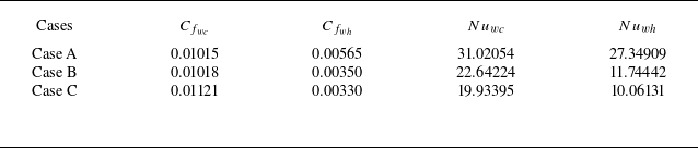
The skin friction coefficient and Nusselt number at the cooled and heated walls, respectively.

Quadrant analysis of density fluctuation contribution
 $\overline {\rho ' v''h''}$
: (a) cooled side, and (b) heated side. Black solid line indicates case A, red dashed line indicates case B, blue dotted line indicates case C.

3.4. Effect of density fluctuation on skin friction coefficient and Nusselt number
Since the effects of density on turbulence and heat transfer, as observed, ultimately manifest in the skin friction coefficient and Nusselt number, we have computed these quantities in table 3. The equations used for these calculations are
 \begin{align} C_{f_{wc}} = \frac {\tau _{wc}^\dagger }{\frac {1}{2} \rho _{b}^\dagger (u_b^\dagger )^2}, \quad C_{f_{wh}} = \frac {\tau _{wh}^\dagger }{\frac {1}{2} \rho _{b}^\dagger (u_b^\dagger )^2},\end{align}
 \begin{align} Nu_{wc} = \frac {2 q_{w}^\dagger \delta ^\dagger }{\lambda _{b}^\dagger | T_{wc}^\dagger - T_{b}^\dagger |}, \quad Nu_{wh} = \frac {2 q_{w}^\dagger \delta ^\dagger }{\lambda _{b}^\dagger | T_{wh}^\dagger - T_{b}^\dagger |},\end{align}
where the subscript ‘b’ refers to the bulk values. Here,
 $ \tau _w^\dagger$
and
 $ q_w^\dagger$
represent the wall shear stress and total wall heat flux, respectively.
Near the cooled wall, where density fluctuations are minimal, the skin friction coefficients
 $ C_{f_{wc}}$
are higher than those of
 $ C_{f_{wh}}$
on the heated wall side, where density fluctuations are more pronounced in all cases. In addition,
 $ C_{f_{wh}}$
continues to decrease with increasing density ratio. This suggests that significant density fluctuations could have a negative effect on the skin friction coefficient. For the Nusselt number, it is observed that
 $ Nu_{wc}$
is larger than
 $ Nu_{wh}$
, which shows that augmented density fluctuations could attenuate the heat transfer at the heated wall. The shear stress and heat flux balances can further facilitate understanding the effect of density fluctuations on skin friction coefficient and Nusselt number. For the shear stress, we derived the stress balance from the mean momentum equation
 \begin{equation} \overline {\mu\, {{\rm d}u}/{{\rm d}y}} - \overline {\rho }\, \widetilde {u''v''} = \overline {\tau }_{{total}}, \end{equation}
where on the left-hand side, the first term represents viscous shear stress, and the second term represents turbulent shear stress;
 $ \overline {\tau }_{{total}}$
represents the total shear stress. The wall-normal distribution of viscous shear stress term is shown in figure 18(a). We observe that the viscous shear stress increases with density ratio at the cold wall, whereas it decreases at the hot wall. In most regions, the viscous shear stress is relatively small compared to the turbulent shear stress (see figure 10
a). As a result, the total shear stress is primarily governed by turbulent shear stress. This finding is consistent with previous work (Nemati et al. Reference Nemati, Patel, Boersma and Pecnik2016b
), which quantified the individual laminar contribution (induced by viscous shear stress) and turbulent contribution (induced by turbulent shear stress) to the total skin friction using the Fukagata–Iwamoto–Kasagi identity (Fukagata, Iwamoto & Kasagi Reference Fukagata, Iwamoto and Kasagi2002). Their results demonstrated that the turbulent contribution is dominant. As shown in § 3.2, our findings reveal that density fluctuations enhance turbulent shear stress at the cold wall but weaken it at the hot wall, which aligns with the skin friction coefficient in table 3. It is reasonable to conclude that density fluctuations affect the total shear stress in a similar manner.
Distributions of (a) viscous shear stress
 $\overline {\mu\, {{\rm d}u}/{{\rm d}y}}$
, and (b) molecular heat flux
 $\overline {\alpha\, {{\rm d}h}/{{\rm d}y}}$
along the wall-normal direction.

A similar analysis is performed on the mean energy equation, yielding the following total heat flux balance:
 \begin{equation} \overline {\alpha\, {{\rm d}h}/{{\rm d}y}} - \overline {\rho }\, \widetilde {v''h''} = \overline {q}_{{total}}, \end{equation}
where on the left-hand side, the first term represents molecular heat flux, and the second term turbulent heat flux;
 $ \overline {q}_{{total}}$
represents the total heat flux. The normal distributions of molecular heat fluxes are shown in figure 18(b). It is found that the molecular heat flux increases with density ratio at the cold wall, whereas it decreases at the hot wall. Furthermore, in most regions, the molecular heat flux is small, and turbulent heat flux (see figure 14
a) dominates the total heat flux, in line with previous findings (Nemati et al. Reference Nemati, Patel, Boersma and Pecnik2016b
). Consequently, it is suggested that the effects of density fluctuations on turbulent heat flux observed in § 3.3 also extend to the total heat flux. That is, the large density fluctuation near the heated wall could exert a negative contribution to the total heat flux (consistent with
 $ Nu_{wh}$
in table 3) by ‘hot ejection’ motions.
3.5. Instantaneous flow characteristics
Instantaneous cross-sectional views (
 $x-z$
plane) of SCP channel flow in case C: (a) cooled wall side at
 $ y^* = 25$
with black contour lines of
 $ \rho ' = -0.1$
, and blue contour lines of
 $ \rho ' = 0.1$
; (b) heated side at
 $ y^* = 16$
with black contour lines of
 $ \rho ' = -0.7$
, and blue contour lines of
 $ \rho ' = 0.4$
.

Iso-surfaces of near-wall (a) low-speed (
 $ u''/u_\infty = -0.15$
) and (b) high-speed (
 $ u''/u_\infty = 0.15$
) structures for case C.

Figure 19 provides snapshots of the streamwise velocity fluctuation
 $ u''$
, wall-normal velocity fluctuation
 $ v''$
, Reynolds shear stress fluctuation term
 $ \rho ' u'' v''$
, and turbulent heat flux term
 $ \rho ' v'' h''$
at
 $ y^* = 25$
(cooled side) and
 $ y^* = 16$
(heated side) on the
 $ x$
–
 $ z$
plane in case C, where
 $ u''$
and
 $ v''$
are normalised using the maximum value of the streamwise velocity,
 $ u_\infty$
. Contour lines represent density fluctuation at prescribed values. In figure 19(a), it can be observed that contour lines at
 $ \rho ' = 0.1$
correspond to the upward low-speed region (
 $ u'' \lt 0$
,
 $ v'' \gt 0$
), while contour lines at
 $ \rho ' = -0.1$
are associated with the downward high-speed region (
 $ u'' \gt 0$
,
 $ v'' \lt 0$
). These regions respectively signify the prevalence of ‘ejection’ and ‘sweep’ events near the cooled wall, where density fluctuation generates additional negative or positive Reynolds shear stress and turbulent heat flux. This observation aligns with the quadrant analysis results. Near the heated wall, as shown in figure 19(b), density fluctuation is stronger, where contour lines at
 $ \rho ' = 0.4$
coincide with the downward high-speed region (
 $ u'' \gt 0$
,
 $ v'' \gt 0$
), and
 $ \rho ' = -0.7$
is highly correlated with the upward low-speed region (
 $ u'' \lt 0$
,
 $ v'' \lt 0$
). These also correspond to ‘sweep’ and ‘ejection’ events near the heated wall, where significant additional Reynolds shear stress and turbulent heat flux are generated.
Figures 20(a) and 20(b) present iso-surface plots of high-speed and low-speed structures, coloured by density fluctuation. It is revealed that on the cooled wall side, the velocity structures with small density fluctuation lift and gradually form horseshoe shapes (red circle), which induces substantial Reynolds shear stress (Robinson Reference Robinson1991). On the heated wall side, the structures with large density fluctuation become sparse and elongated (orange circle). Thus the Reynolds stress is suppressed.
4. Conclusions
Direct numerical simulations are conducted on turbulent channel flow of supercritical pressure (SCP) CO
 $_2$
with cooled and heated isothermal walls. The substantial wall temperature difference induces strong real-fluid effects related to density fluctuation. The investigation aims to elucidate how large density fluctuation impacts near-wall turbulence and turbulent heat transfer in fully developed channel flow at SCP by employing various analytical techniques.
It is found that at the cold wall, density fluctuation is minimal, and the turbulence characteristics are similar to those at atmospheric pressure. However, on the hot wall side, where the pseudo-boiling temperature point is located, density fluctuation exhibits a notable impact with increasing density ratio, contributing approximately 12 % to first-order moments, and 30 % to second-order moments. Consequently, Morkovin’s hypothesis is found to be invalid in this context.
Decomposition of the statistics and budget analysis reveals that large density fluctuation induces additional turbulent mass transfer
 $\overline {u_i''}$
, which contributes positively to TKE. However, it also diminishes the turbulence production simultaneously, resulting in an overall reduction in TKE. The quadrant analysis further elucidates the complex mechanisms by which density fluctuations influence Reynolds shear stress across different turbulence events, providing deeper insights. Specifically, the ‘ejection’ events dominated the contribution to Reynolds shear stress, with density fluctuation contributing positively on the cooled wall side and negatively on the heated wall side. As the total shear stress is dominated by turbulent shear stress in most regions, this indicates that density fluctuations affect the total shear stress (skin friction coefficient) in a similar manner.
As for turbulent heat transfer, the wall-normal turbulent heat flux production is primarily balanced by the enthalpy–pressure-gradient correlation in the cooled wall, while a net increase is still observed. In proximity to the heated wall, the enhanced density fluctuation induced
 $\overline {h''}$
induces a notable increase in the enthalpy–pressure-gradient correlation term, which diminishes the wall-normal turbulent heat flux. However, the additional terms from large density fluctuation, as well as the molecular diffusion term from the fluctuations in thermal conductivity and isobaric specific heat capacity, offset the reduction. The quadrant analysis of turbulent heat flux reveals that the overall negative contribution of the density fluctuation near the heated wall stems primarily from ‘hot ejection’ motions. Since in most regions, turbulent heat flux dominates the total heat flux, it is suggested that the effects of density fluctuations on turbulent heat flux observed here also extend to the total heat flux (Nusselt number).
The snapshots of flow structures demonstrate that large density fluctuations tend to be associated with regions characterised by significant additional Reynolds shear stress and turbulent heat flux, providing further support for quadrant analysis. Furthermore, it is revealed that velocity structures with small density fluctuations lift and gradually form horseshoe shapes, inducing substantial Reynolds shear stress. In contrast, velocity structures with large density fluctuations become sparse and elongated, which could explain the decrease in Reynolds shear stress near the heated wall.
Acknowledgements.
The authors thank Professor C. Sun for valuable suggestions on the overall research, and acknowledge the help of the Computing Center in Xi’an.
Funding.
This work is supported by the National Natural Science Foundation of China (52276123), the China Postdoctoral Science Foundation (2024M751636), the National Science and Technology Major Project (Y2019-I-0022-0021), the Postdoctoral Fellowship Program of CPSF (GZC20231221), the Anhui Provincial Natural Science Foundation (2308085MA27), and the National Key Laboratory of Ramjet Fund.
Declaration of interests.
The authors report no conflict of interest.
Data availability statement.
The data that support the findings of this study are available from the corresponding author upon reasonable request.
Appendix A. Quantitative effects of density fluctuation
The contribution of density fluctuation to the first-order statistical quantities is first examined quantitatively. Leveraging the relationship between the Reynolds averaging and Favre averaging of a physical quantity
 $\phi$
, the fluctuating component in Favre averaging,
 $\overline {\phi ''}$
, can be easily derived:
 \begin{equation} -\frac {\overline {\phi ''}}{\overline {\phi }} = \frac {\widetilde {\phi } - \overline {\phi }}{\overline {\phi }} = \frac {\overline {(\bar {\rho } + \rho ') (\bar {\phi } + \phi ')}}{\overline {\rho } \, \overline {\phi }} - 1 = \frac {\overline {\rho ' \phi '}}{\overline {\rho } \, \overline {\phi }}. \end{equation}
Based on (A1), the relative impact of density fluctuation on the physical quantities, such as velocity components and enthalpy, can be effectively analysed. Figures 21(a) and 21(b) show the distributions of
 $-\overline {u''} / \overline {u}$
and
 $-\overline {h''} / \overline {h}$
along the wall-normal direction. Near the cooled wall, the fluid is distant from the pseudo-boiling temperature. Both
 $-\overline {u''}$
and
 $-\overline {h''}$
induced by density fluctuation are within 2 % of their mean quantities, thus the effect of density fluctuation is negligible in the proximity of the cooled wall. On the other hand, near the heated wall, where the flow experiences transcritical process, the influence of density fluctuation remains minor in case A with small density ratio. Yet in cases B and C characterised by large density ratio, the impact of density fluctuation on first-order statistics becomes significant and increases up to fourfold (approximately 12 %). Physically,
 $\overline {\rho ' \phi '}$
represents the correlation between the fluctuations of density and physical quantity. It is thus important to consider the effects of the density fluctuation on time-averaged momentum and energy transports when the transcritical phenomenon occurs.
Contribution of density fluctuation to (a) mean velocity and (b) mean enthalpy. Black solid line indicates case A, red dashed line indicates case B, blue dotted line indicates case C.

Effects of density fluctuation on (a)
 $\overline {u'u'}$
, (b)
 $\overline {v'v'}$
, (c)
 $\overline {w'w'}$
, (d)
 $\overline {u'v'}$
, and (e)
 $\overline {v'h'}$
. Black solid line indicates case A, red dashed line indicates case B, blue dotted line indicates case C.

We continue to quantitatively analyse the effect of the large density fluctuation on second-order turbulence statistics. Equation (A1) can be rewritten in terms of fluctuating components:
 \begin{equation} \phi '' = \phi ' - \frac {\overline {\rho ' \phi '}}{\overline {\rho }}. \end{equation}
Substituting two physical quantities
 $\phi _1$
and
 $\phi _2$
into (A2), a difference in second-order statistics,
 $\widetilde {\phi _1'' \phi _2''}- \overline {\phi _1' \phi _2'}$
, can be derived:
 \begin{equation} \widetilde {\phi _1'' \phi _2''} - \overline {\phi _1' \phi _2'} = \frac {\overline {\rho ' \phi _1' \phi _2'}}{\overline {\rho }} - \frac {\overline {\rho ' \phi _1'} \times \overline {\rho ' \phi _2'}}{\overline {\rho }^2}. \end{equation}
The left-hand side of (A3) is the difference between Favre- and Reynolds-averaged second-order moments, which can be interpreted as the difference between a third-order moment and a product of two second-order moments on the right-hand side. Equation (A3) clearly shows the role of density fluctuation in second-order statistics in variable-density flows. Substituting the velocity components into (A3), the Reynolds stresses (per unit mass) in Favre- and Reynolds-averaged forms
 $\widetilde {u_i'' u_j''}$
and
 $\overline {u_i' u_j'}$
are obtained. The right-hand side of (A3) thus signifies the impact of density fluctuation on Reynolds stresses. Figures 22(a–d) illustrate the distributions of relative difference between Favre- and Reynolds-averaged normal and shear stresses in the wall-normal direction (
 $y$
). Near the cooled wall (
 $y\lt 0.2$
), a relatively small discrepancy between Favre- and Reynolds-averaged stresses is observed because of small density fluctuation (figure 6
a). In contrast, near the heated wall (
 $y \gt 1.75$
), the relative difference becomes more pronounced. Such a trend coincides with that of density fluctuation in figure 6(b). Higher amplitude of density fluctuation produces larger relative difference in stresses. The relative difference in shear stress induced by density fluctuation reaches up to 15 % in case C (figure 22
d). Figure 22(e) shows that density fluctuation exerts an even greater impact on turbulent heat flux, with up to 70 % of
 $\overline {v' h'}$
in proximity to the heated wall in case C. The large density fluctuations could also be related to the high Prandtl number near the hot wall. The thinning of the thermal boundary layer intensifies the thermophysical gradients, contributing to heightened thermophysical fluctuations near the wall. This also challenges the traditional mean velocity and temperature scaling law (Karman & Howarth Reference Karman and Howarth1938; Kader Reference Kader1981), as shown in figure 23.
The r.m.s. of each term in the
 $x$
-momentum equation.

(a) Mean velocity
 $ \bar {u}^+$
, and (b) mean temperature
 $ \bar {T}^+$
, as functions of
 $ y^+$
, where
 $ \bar {u}^+ = {\bar {u}}/{\bar {u}_\tau }$
and
 $ \bar {T}^+ = {\bar {T}}/{\bar {T}_\tau }$
. Here,
 $ \bar {u}_\tau$
and
 $ \bar {T}_\tau$
are the wall friction velocity and friction temperature, respectively, and
 $ Pr_{w}$
is the Prandtl number at the wall.

Appendix B. Validation
The present work considered fully developed channel flows, and did not cover buoyancy effect for two primary reasons. First, by initially excluding buoyancy, we can isolate the effect of density fluctuations on turbulence statistics of SCP fluids under standard flow conditions (i.e. forced convection), and also enable easier validation or comparison with other studies. Many other fundamental studies on fully developed channel flows at SCP can be found with forced convection in the open literature, such as Ma et al. (Reference Ma, Yang and Ihme2018), Guo, Yang & Ihme (Reference Guo, Yang and Ihme2022) and Li et al. (Reference Li, Pei and Bai2022); these studies considered similar temperature differences and density ratios. Second, we have performed a brief analysis to evaluate the contribution of the buoyancy term. In the case with temperature difference 150 K (case C), for example, the following parameters were used: bulk velocity
 $ u_{b}^\dagger = 0.405 \, \text {m}\,{\rm s^-{^1}}$
, channel half-height
 $ \delta ^\dagger = 0.5 \, \text {mm}$
, and gravity
 $ g^\dagger = -9.8 \, \text {m}\,{\rm s^-{^2}}$
(opposite to the flow direction). The corresponding inverse of the Froude number is
 $ {1}/{Fr} = -0.02987$
. After 20 flow-through times, we performed an order of magnitude analysis of the instantaneous data using r.m.s. statistics. The r.m.s. of a generic variable
 $ \phi$
is calculated as
 \begin{equation} \phi _{\textit {rms}} = \sqrt {\frac {1}{N} \sum _{i=1}^{N} (\phi ^i)^2 }, \end{equation}
where
 $ N$
is the total number of grids, and
 $ \phi ^i$
is the value of
 $ \phi$
in the
 $ i$
th grid. The results of the order of magnitude analysis for the terms in the streamwise momentum equation are summarised in table 4. The buoyancy term was found to be two orders of magnitude smaller than the convective term, and one order of magnitude smaller than the viscous and pressure gradient terms. This suggests that the contribution of buoyancy is minimal in comparison to other terms.
(a) Mean velocity profile and (b) r.m.s. of velocity fluctuations. Lines indicate present code, and symbols indicate data obtained from the work of Kawamura, Abe & Matsuo (Reference Kawamura, Abe and Matsuo1999).

Simulation results for strongly heated internal gas flow at
 $ {Re}_0 = 6000$
: (a) mean velocity profile, and (b) mean temperature profile along the radial direction. Lines represent code results, and symbols represent experimental data obtained from the work of Shehata & McEligot (Reference Shehata and McEligot1998). Note that the abscissa is shifted upwards for each curve.

Our code has been validated using DNS data from Kawamura et al. (Reference Kawamura, Abe and Matsuo1999) and experimental data from Shehata & McEligot (Reference Shehata and McEligot1998). Figures 24(a) and 24(b) compare the mean velocity
 $ \overline {u}$
and r.m.s. of velocity fluctuations
 $ u'_{\textit {irms}}$
with
 $ \textit {Re}_\tau = 180$
and
 $ \textit {Pr}_w = 0.71$
, where
 $ y^{\text {+}}$
and
 $ \overline {u}_\tau$
represent the wall-normal coordinate normalised by the viscous scale and the friction velocity, respectively. The results show excellent agreement with those of Kawamura et al. (Reference Kawamura, Abe and Matsuo1999), confirming the validity of the current DNS methodology. Figures 25(a) and 25(b) compare the radial (
 $ r$
) profiles of mean streamwise velocity
 $ \overline {u}_{x}$
and temperature
 $ \overline {T}$
at different axial locations from our prior DNS data with the experimental data from Shehata & McEligot (Reference Shehata and McEligot1998). The comparison again shows excellent agreement, validating the accuracy of the thermophysical property calculation methods used in this study. The correctness of both DNS methodology and thermophysical property calculation could guarantee the accuracy of the present DNS study at SCP. More details can be found in Zhao et al. (Reference Zhao, Wan, Jin, Chen, Li and Peng2021).