3.1. Wind tunnel

All tests were performed in an air-breathing supersonic wind tunnel of the National Key Laboratory of Science and Technology on Aerodynamic Design and Research at Northwestern Polytechnical University (NPU). The nominal free-stream Mach number was 4.2 at the exit of the nozzle. The facility comprised a stagnation chamber with damping screens, an interchangeable rectangular supersonic nozzle, a test section, a diffuser, and a $200\ \text {m}^3$ vacuum tank, as shown in figure 2. Four vacuum pumps could pump the vacuum tank to a pressure of less than $0.1\ \text {Pa}$ in 1 h. These settings enabled sustained runs of approximately $10\ \text {s}$.

Figure 2.

Diagram of the supersonic facility at NPU.

The entrance of the test section measured $200\ \text {mm}\times 200\ \text {mm}$ (${\rm width} \times {\rm height}$). The divergence of the upper and lower walls in the test section was adjusted by $\pm 0.5^{\circ }$ relative to the centreline, considering the development of the boundary layer along these walls. The test section contained removable modules on all four sides to mount the models and provide optical access. Two pieces of optical glass of dimensions $260\ \text {mm}\times 180\ \text {mm}$ were mounted on each sidewall for schlieren imaging.

The flow conditions used in this study are listed in table 1. Here, $M_{\infty }$, $T_{0}$ and $P_{0}$ correspond to the nominal Mach number, stagnation temperature and stagnation pressure of the supersonic flow at the exit of the nozzle, and $U_{1}$ denotes the edge velocity on the flat plate upstream from the STBLI region. The Mach number at the flat plate, denoted as $M_{1}$, is $4.1\pm 0.02$, slightly lower than the free-stream Mach number 4.2, resulting in a unit Reynolds number $Re^{*}=4.3\times 10^{6}\ \text {m}^{-1}$. This discrepancy can be attributed to the deceleration caused by a shock generated by the forced transition device positioned at the leading edge of the flat plate.

Table 1.

Summary of flow conditions.

3.2. Test model

Figure 3 provides a schematic representation of the model. A full-span, 610 mm long steel plate with a $5^{\circ }$ lead was employed to generate the boundary layer for all tests. The plate was connected to the bottom wall at height $60\ \text {mm}$ by using a rib plate. The rib plate was specifically designed to offset the divergence angle of the lower wall. Therefore, the full-span plate was parallel to the free-stream flow. The forced transition method was also employed to facilitate the boundary layer transition and to ensure a turbulent boundary layer upstream from the STBLI zone. The downstream STBLI was produced by using a compression corner with deflection angle $24^{\circ }$ at the end of the plate. The upstream STBLI was generated by employing a two-dimensional wedge suspended from the upper wall. Different angles were designed to achieve disparate shock intensities. The vertical distance between the tip of the wedge and the plate surface was $80\ \text {mm}$. This wedge could be moved streamwise in $10\ \text {mm}$ intervals, resulting in different distances between the two STBLI regions.

Figure 3.

Diagram of the test section, with plate model, wedge and the distribution of pressure transducers.

As shown in figure 3, the incident shock $i$ intersects the centreline of the plate surface at point $o_{1}$ under inviscid conditions. The distance between $o_{1}$ and $o_{2}$ (the origin of the ramp at the end of the plate) is defined as $d$. The configurations of the two cases are presented in table 2, with the upstream deflection angles of the wedge being $3^{\circ }$ and $10^{\circ }$. The shock generator was adjusted with a spacing of approximately $10\ \text {mm}$ along the flow direction during the test to obtain six distances between the impingement point of the incident shock and the origin of the compression corner. The values of $d$ obtained from schlieren imaging are also listed in table 2.

Table 2.

Geometric parameters of test model.

3.3. Test programme

Different diagnostic methods were used throughout the tests. The tests aimed to determine the flow structure of the interference between the two interaction regions and to provide a physical interpretation. High-frequency pressure measurements were used to investigate the unsteadiness and communication between the two interaction regions. Although commonly utilised for qualitative analysis, the schlieren imaging technique directly correlates the light intensity of the schlieren image with the density gradients in the flow, thereby providing valuable information. The evaluation of the flow oscillation frequencies can be facilitated by utilising time-resolved flow field information. High-speed schlieren imaging is a superior method of acquiring extensive datasets. The PIV measurements were also utilized to quantitatively characterise the state of the boundary layer through its interactions with shock waves.

3.4. Upstream turbulent boundary layer

The flow parameters of the undisturbed boundary layer were determined by utilising measurements from PIV. The measurements were conducted $380\ \text {mm}$ from the leading edge of the plate. The mean velocity profile is presented in figure 4(a). The incompressible theory is extended to include compressible flows by modifying the dimensional analysis to account for changes in density using the van Driest effective velocity (van Driest Reference van Driest1951). Subsequently, this velocity is combined with the Walz equation (Walz Reference Walz1969) and the perfect gas law, assuming a constant pressure throughout the boundary layer. This integration yields a closed-form equation

Figure 4.

Turbulent boundary layer conditions. (a) Velocity profile of the upstream turbulent boundary layer obtained by PIV and Pitot tube. (b) The PSD based on wall pressure (blue) and the coherence $C_{xy}$ (red) between the wall pressure within the upstream boundary layer and separation. The grey shaded area indicates the region outside sensor frequency response (>40 kHz).

(3.1)\begin{equation} u^* = \frac{u_{e}}{b}\sin^{{-}1}\left(\frac{2b^2(u/u_{e})-a}{\sqrt{(a^2+4b^2)}}\right), \end{equation}

where

(3.2)$$\begin{gather} a=\left(1+r\,\frac{\gamma-1}{2}\,{M_{e}}^2\right)\frac{T_{e}}{T_{w}}-1, \end{gather}$$

(3.3)$$\begin{gather}b^2=r\,\frac{\gamma-1}{2}\,{M_{e}}^2\left(\frac{T_{e}}{T_{w}}\right), \end{gather}$$

and $r=Pr^{1/3}=0.89$ represents the recovery factor. For the case of an adiabatic zero-pressure-gradient flat-plate compressible turbulent boundary layer, when the recovery temperature is equal to the wall temperature, we have $a=0$. And the velocity profile in the log layer is defined as

(3.4)\begin{equation} {u_{vd}}^+ = \frac{u^{*}}{u_{\tau}}=\frac{1}{\kappa}\log\left(\frac{u_{\tau}y}{\upsilon}\right)+C, \end{equation}

where $\kappa =0.41$ and $C=5.2$. Coles (Reference Coles1956) extended the log law into the outer scaling region by adding a wake function to describe the departure from the log layer. The derived law of the wake,

(3.5)\begin{equation} {u_{vd}}^+ = \frac{1}{\kappa}\log \left(\frac{u_{\tau}y}{\upsilon_{w}}\right)+C+\frac{2\varPi}{\kappa}\sin^2\left(\frac{\rm \pi}{2}\,\frac{y}{\delta_{1}}\right), \end{equation}

remains applicable throughout the logarithmic layer to the outer region, encompassing the intermediate overlap.

The statistical uncertainty associated with the mean velocity, due to limited realisations, is less than $1\,\%\,U_{1}$. The transformed velocity profile matches well with the standard log law, and a distinct wake component characteristic of turbulent boundary layers can be identified clearly, which aligns with Coles’ law of the wake (Coles Reference Coles1956). The friction velocity was obtained by making a least squares fit to the law of the wake of the measured velocity profile. According to the PIV data, the boundary layer thickness $\delta _{1}$ measured $8.8\ \text {mm}$ $(99\,\%\,U_{1})$, while the displacement thickness $\delta _{1}^{*}$ was found to be $3.6\ \text {mm}$. The momentum thickness $\theta$ was determined as $0.4\ \text {mm}$, and the shape factor $H$ was calculated as 8.2. Additionally, the Reynolds number $Re_{\theta }$ based on momentum thickness was estimated at $1.9\times 10^3$. These flow conditions are summarised in table 3. The reference flow is further documented by presenting a sample PSD graph in figure 4(b), which illustrates the wall pressure within the undisturbed boundary layer. The fluctuation energy remains broad and consistent across the low-frequency range, which is in accordance with the results of high-speed flow experiments conducted by Beresh et al. (Reference Beresh, Henfling, Spillers and Pruett2011). Furthermore, we examined the potential correlation between the pressure fluctuations in the incoming flow and those in the recirculation region. Figure 4(b) illustrates the coherence between the wall pressure measurements within the incoming boundary layer and at the separation shock foot. This coherence suggests that a minimal correlation exists between the pressure fluctuations in the upstream boundary layer and low-frequency unsteadiness near the separation.

Table 3.

Summary of flow conditions.

4.1. Expanded separation: the role of a retarded boundary layer

Time-averaged schlieren images were used to investigate the overall separation trends of the interactions. The interference between weak interacting flows originating from different upstream shock impact locations and a strong STBLI is illustrated in figure 5. Furthermore, the mean wall pressure normalised by the free-stream pressure and the relative standard deviation $\sigma _{p}/p_{w}$ along the centreline for each case are also presented. The incident shock $i$, as shown in figure 5(a), impacts approximately $52\ \text {mm}$ upstream from the origin of the compression corner ($x=0\ \text {mm}$). For ease of comparison in the subsequent cases, we define the impinging location as the intersection between the incident shock extension line and the wall surface in the inviscid flow; however, because of the upstream bending of the incident shock beneath the boundary layer, the actual shock foot is positioned $5\ \text {mm}$ upstream from this impinging location. Reflected shock $ii$ is relatively weak because of the small deflection angle of the wedge. The nominal Mach number downstream from the first STBLI region was 3.89, and the compression-ramp-induced STBLI led to a separated boundary layer. The wall pressure distribution reveals the presence of two pressure increases: one caused by the incident shock, and the other induced by the shock at the compression corner. The separation point captured by the schlieren image is approximately $6\ \text {mm}$ upstream from the corner. The local maxima for $\sigma _{p}/p_{w}$ can be employed to identify the shock foot. The peak observed at T7 may have been caused by a spanwise shock wave that occurred because of the gap between the test section and either the nozzle or the window. The interaction extent $L_{{ext}}$, which is defined as the distance between the origin of the interaction and the location of the separation point of the compression-ramp-induced STBLI identified by wall pressure measurements, is approximately $15\ \text {mm}$.

Figure 5.

Distributions of wall pressure and relative standard deviation for case A with different spacings between the two interaction regions, along with the mean flow structures: (a) $d=52\ \text {mm}$, (b) $d=30\ \text {mm}$, (c) $d=19\ \text {mm}$, (d) $d=10\ \text {mm}$.

When the incident shock shifts $10\ \text {mm}$ downstream ($d=41\ \text {mm}$), besides the displacement of the incident shock and slight expansion of the separation region, no significant changes are observed in the flow field depicted in figure 5(a); therefore, detailed flow information is not provided here. Notably, even though the upstream STBLI is relatively weak, the turbulence in the incoming boundary layer is distorted by its passage across the shock wave, then is convected downstream and contributes to the formation of a new boundary layer. In addition, the adverse pressure gradient caused by the incident shock cannot be ignored. The STBLI at the compression corner encounters a progressively incomplete boundary layer as the incident shock moves downstream. The presence of such a disturbed boundary layer (retarded boundary layer) is thought to affect the flow parameters at the downstream separation, such as shear stress. According to the free-interaction theory, these flow parameter variations can affect both the initial pressure increase and the length of the region associated with the separation. However, owing to either the limitations in the transducer distribution or a relatively weak STBLI, no significant effect is observed, and $L_{{ext}}$ remains unchanged in these two scenarios.

The incident shock in figure 5(b) shifts further downstream with $d=30\ \text {mm}$, and the downstream STBLI also undergoes a significant change in this scenario. Notably, although the displacement of the shock foot remains consistent with the previous observations ($d$ changes from 52 mm to 41 mm and then to 30 mm, corresponding to a variation of 5 mm in the shock foot position towards upstream), a sudden and substantial increase in $L_{{ext}}$ occurs, where $L_{{ext}}$ reaches $40\ \text {mm}$. This length is more than twice the previous length. Additional shock waves for which the origin location (time-averaged) is consistent with the upstream influence (UI) are more perceptible in this scenario. The intensity and shock angle at the UI are greater for the downstream interaction than for the upstream one, indicating that flow deflection exceeds that caused by the upstream shock. The gradual rise in pressure towards the separation point can be attributed to both the combination of the incident shocks and the UI resulting from the downstream STBLI.

The incident shock in figure 5(c) undergoes a displacement of an additional $10\ \text {mm}$. In the absence of interference between the two interaction regions, the impingement point of the upstream incident shock should ideally align with the starting point of the UI as shown in figure 5(a). However, the time-averaged schlieren image reveals a significant change in the origin of the compression wave as it crosses the impinging point of the upstream incident shock. Despite this difference, no shift in the location of the separation point identified by the schlieren image compared with that depicted in figure 5(b) is apparent. The peak position of $\sigma _{p}/p_{w}$ also exhibits a notable displacement, which is consistent with the alterations observed in the schlieren image depicting the compression wave. The significant reduction in the skin friction coefficient within the interaction region is a crucial characteristic of the STBLI, and based on the free-interaction theory, the interaction extent $L_{{ext}}$ is inversely proportional to the skin friction coefficient. From this phenomenon, we can infer that the upstream STBLI region overlaps with the initial portion of the downstream STBLI region. The sudden change in $L_{{ext}}$ results from drastic changes in the local flow conditions at the separation point of the downstream STBLI. An evident extension of the separation is observed in figure 5(d), whereas the length $L_{{ext}}$ appears to be consistent with that in figure 5(a). In this scenario, the shock foot has already passed the impingement point of the upstream incident shock; thus the incident shock no longer affects the flow parameters at separation.

Even with a small deflection angle, the impact of the incident shock is evident. Figure 6 illustrates the variation in the shock foot position at the compression corner in case A. Initially, the shock foot position changes linearly with $d$, which aligns with the gradual variations in the flow parameters within the boundary layer downstream from the first STBLI region. However, when $d$ reaches $19\ \text {mm}$, a shift in the shock foot position occurs. According to the free-interaction theory, the local flow parameters affect the extent of the interaction, resulting in changes in the UI; however, the local flow does not affect the separation. The superposition of pressure gradients also plays a crucial role in this situation. A greater length is required for the development of the separation shear layer (flow acceleration) to achieve a larger pressure increase. In addition, the separation can be facilitated by the presence of a retarded boundary layer following the interaction region.

Figure 6.

Variation of the shock foot position in case A. These locations were determined according to the peak of the relative standard deviation.

The mean flow behaviour is also described by the average streamwise velocity field in figure 7(a). The contour lines are densely distributed around dimensionless velocity 1.0, making the incident shock visible despite its relatively weak intensity. The distorted boundary layer downstream from the first STBLI region seems to exhibit a gradual increase in thickness at a relatively modest rate. The profiles of the streamwise velocity in the wall-normal direction at $x=25\ \text {mm}$ are shown in figure 7(b). When the first STBLI is at a distant location, such as $d=52$ and $30\ \text {mm}$, no significant change occurs in the boundary layer state upstream from the interaction region at the compression corner. However, when the incident shock continues to move downstream ($d=19\ \text {mm}$), a notable deficit is observed in the streamwise velocity. This deficit caused by an adverse pressure gradient could be due to either the upstream incident shock or forward propagation of the adverse pressure gradient from the downstream interaction region. The comparison of the first two scenarios reveals that even in the latter case, the deficit in the velocity profile is ultimately attributed to the alteration of the local boundary layer state caused by the upstream incident shock wave.

Figure 7.

Mean streamwise velocity distribution $\bar {u}/U_1$ in case A. (a) Streamwise velocity contours from $-0.2$ to 0.9 in increments of 0.1, and from 0.9 to 1.0 in increments of 0.01. (b) Streamwise velocity profiles with various $d$ at $x=-25\ \text {mm}$.

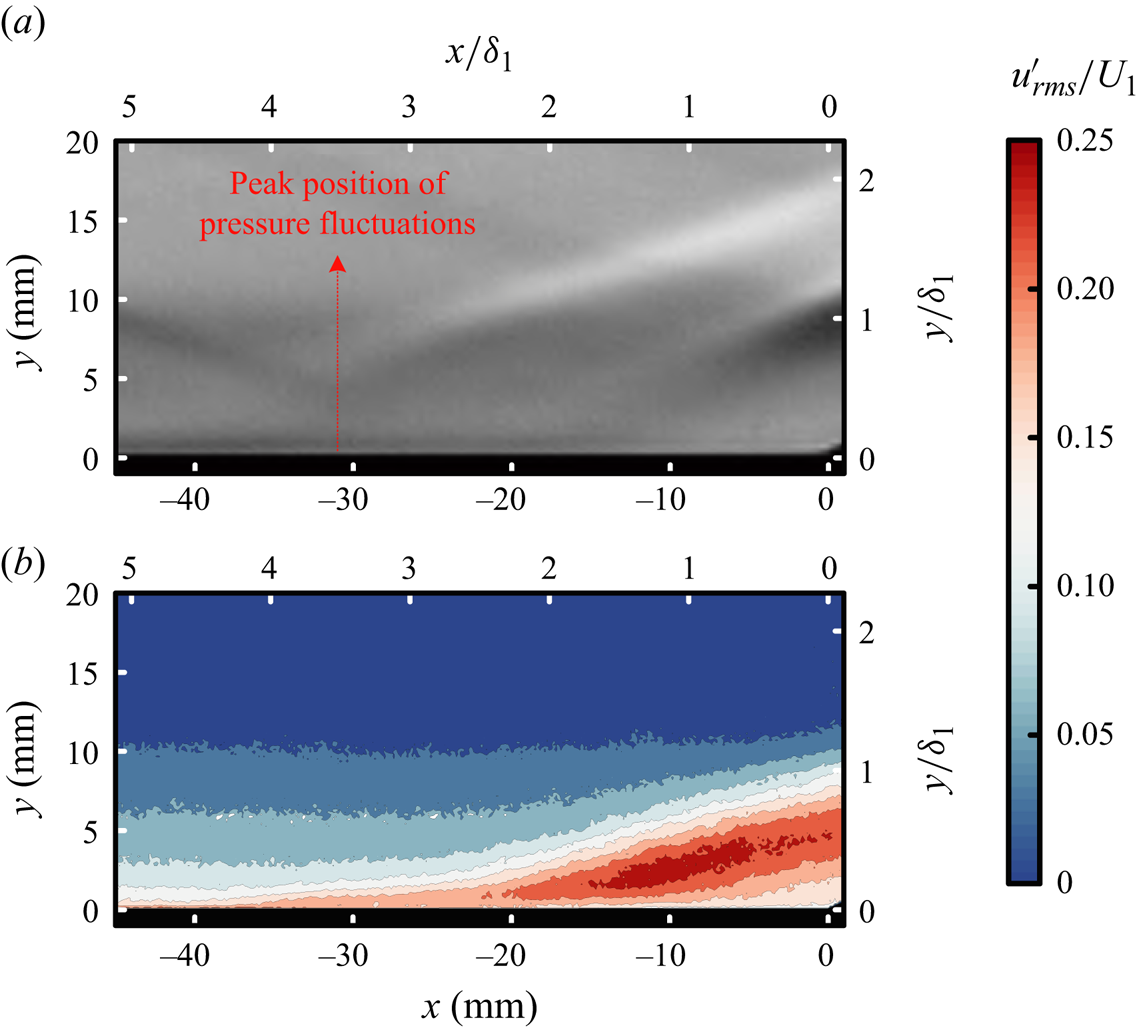
In the scenario in which $d=19\ \text {mm}$, small-field-of-view PIV measurements were conducted in the region between $x= -40\ \text {mm}$ and $x=0\ \text {mm}$. The root mean square (r.m.s.) of the streamwise velocity fluctuations is shown in figure 8, together with the locally magnified schlieren image. A region of high-energy fluctuations, starting at approximately $x= -15\ \text {mm}$, is observed in the r.m.s. contour, indicating the initiation of the shear layer within the separation. Furthermore, fluctuations with a specific level extend upstream to the vicinity of $x= -30\ \text {mm}$, which corresponds to both the peak position of the pressure fluctuation and the area encompassed by the compression waves. These compression waves exhibit a remarkable unsteady behaviour, which will be analysed in the subsequent section on shock unsteadiness.

Figure 8.

Comparison of (a) time-averaged schlieren image and (b) r.m.s. streamwise velocity fluctuations in the magnified field of the interaction region with $d=19\ \text {mm}$.

4.2. Expanded separation: the role of a relaxing boundary layer

This situation differs when the relative positions of the two interaction regions change. In this case, the interaction with the separation occurs upstream. The incident shock impacts a location approximately $56\ \text {mm}$ upstream from the origin of the compression corner, as shown in figure 9(a). Owing to the relatively large deflection angle of the wedge, the incident shock is sufficiently strong to induce a separate boundary layer in the first STBLI region. The nominal Mach number downstream from this region is 2.85. The compression-ramp-induced STBLI leads to a boundary layer without any apparent separation, even at deflection angle $24^{\circ }$. A potential explanation is that the upstream expansion waves induced by the shock generator exert a beneficial influence on the downstream STBLI region. The shock foot, identified using the relative standard deviation, is located near transducer T6. This location aligns with the results of the schlieren image analysis. The absence of a pressure plateau in the pressure distribution can be attributed to the relatively weak incident shock at this Mach number, despite inducing separation. According to Xue et al. (Reference Xue, Jiao, Wang and Cheng2023), under the current flow conditions, the critical flow deflection angle is $24.8^{\circ }$, beyond which further increases in pressure may cease and the pressure may exhibit non-monotonic changes, potentially approaching a plateau.

Figure 9.

Distributions of wall pressure and relative standard deviation for case B with different spacings between the two interaction regions, along with the mean flow structures: (a) $d=56\ \text {mm}$, (b) $d=45\ \text {mm}$, (c) $d=36\ \text {mm}$, (d) $d=25\ \text {mm}$.

When the incident shock shifts $10\ \text {mm}$ downstream, as shown in figure 9(b), the separated STBLI region approaches the downstream region while simultaneously experiencing a similar displacement of the shock foot position. Wall pressure continuously increases from the UI to the compression surface. Furthermore, with the emergence of compression waves, the sonic line gradually moves away from the wall as the flow develops. This observation suggests a change in the subsonic region beneath the boundary layer between these two regions. However, subsequent analysis of the shear layer evolution indicated that a complete connection was not established. As shown in figure 9(c), the incident shock shifts further downstream, making the connection between the two interaction regions more evident. A distinctly separated boundary layer between the two regions can be observed in the schlieren image. The extension of the shock waves towards the lower part of the boundary layer ceases to occur at the compression corner.

In figure 9(d), the incident shock undergoes a downstream shift of an additional $10\ \text {mm}$, resulting in an enlarged merged separation region compared with that in the previous scenario. Simultaneously, a pressure plateau is observed in the wall pressure distribution, which is equal to the value estimated using free-interaction theory. However, the pressure plateau does not extend to the compression corner; instead, it terminates at the location of vortex shedding and is followed by a gradual increase in pressure until it reaches the compression surface because of the compression waves upstream from the reattachment shock. The shock foot moves upstream once again towards transducer T5. In the scenarios with $d=16$ and $6\ \text {mm}$, the separation shock gradually moves upstream as the incident shock progresses downstream, and the size of the separation region continuously expands. The presence of pressure plateaus also become more prominent, coinciding with the increasing platform area.

The average streamwise velocity fields for case B are displayed in figure 10(a). For the scenario in which $d=56\ \text {mm}$, the velocity profiles at different streamwise locations downstream from the first STBLI region are presented in figure 10(b). When the two interaction regions are far apart, the downstream boundary layer develops with a relatively low rate of recovery until it reaches the compression corner. When the incident shock moves downstream, it fails to reach the UI of the downstream interaction region starting at approximately $x=-11\ \text {mm}$. The adverse pressure gradient initially affects the relaxing boundary layer from downstream, causing a gradual displacement of the sonic line within this boundary layer away from the wall, and resulting in a sequence of compression waves in the second STBLI region. As the interaction regions approach each other ($d=36\ \text {mm}$), the PIV results reveal a clear connection between the low-energy fluids in the two regions. Furthermore, the schlieren images demonstrate the fusion of the two separation zones, as illustrated in figure 9(c). From this spacing, a reverse movement is observed for the separation shock of the first STBLI. At this point, the adverse pressure gradient induced by the compression corner influences the upstream region through a separated boundary layer. The combined influence of these factors results in the expansion of the separation zone and transition of the reattachment position.

Figure 10.

Mean streamwise velocity distribution $\bar {u}/U_1$ in case B. (a) Streamwise velocity contours from $-0.2$ to 0.9 in increments of 0.1, and from 0.9 to 1.0 in increments of 0.01. (b) Evolution of streamwise velocity profiles at various positions with $d=56\ \text {mm}$.

Overall, the boundary layer between the two STBLI regions plays an important role in the separation expansion. Even with a small deflection angle, the incident shock decelerates the boundary layer, leading to significant changes in the UI and peak position of pressure fluctuations. Downstream from the separated STBLI, the relaxing boundary layer develops with a relatively low rate of recovery and is easier to separate when subjected to adverse pressure gradients. The adverse pressure gradient is more likely to propagate upstream through these perturbed boundary layers when the two interaction regions approach each other, rather than through fully developed turbulent boundary layers.

5.1. Streamwise evolution of the PSD

At each transducer, the pressure was normalised with respect to $p_{\infty }$, and the PSD of the wall pressure was computed over each run to characterise the streamwise variations of the wall pressure dynamics. Figure 11 presents maps of the frequency-premultiplied PSD ($\,f\, G(f)$) of the pressure fluctuations for case A. The spectra are normalised by the variance of the local wall pressure below $40.0\ \text {kHz}$. To enable interpretation with reference to the boundary layer time scales, the right-hand axis in the spectra is shown in terms of $St_{\delta }=f\delta _{1}/U_{1}$. We also give the non-dimensional frequency based on the interaction length $L_{{int}}$ in the subsequent analysis. In all cases, the peak energy should be located at the convection frequency $(U_{1}/\delta _{1}=89.51\ \text {kHz})$; however, these peaks fall near $40\ \text {kHz}$, which is the cutoff frequency of the transducer.

Figure 11.

Streamwise evolution of frequency-premultiplied pressure fluctuation PSD for case A with (a) $d=52\ \text {mm}$, (b) $d=30\ \text {mm}$, (c) $d=19\ \text {mm}$, (d) $d=0\ \text {mm}$. All plots have the same spatial coordinates ($x$–$y$ plane) scaled by the boundary layer thickness and contour levels.

The presence of a weak low-frequency component can be observed at a fixed position between $x=-100\ \text {mm}$ and $x=-80\ \text {mm}$ in figure 11(a), which is consistent with the occurrence of the peak in the distribution of $\sigma _{p}/p_{w}$ in figure 5. This unexpected disturbance can be attributed to the spanwise developing shock caused by the gap between the optical window and the sidewall. Downstream from this region, oscillations induced by the incident shock can be observed within the frequency range from $1.0\ \text {kHz}$ to $5.0\ \text {kHz}$. At the mean location of the shock foot $(x\approx -20\ \text {mm})$, the low-frequency content caused by the STBLI at the compression corner is also detected, and downstream from this interaction region, the broadband peak shifts towards higher frequencies. As the incident shock moves downstream, as illustrated in figures 11(b,c), no significant change is evident in the high-frequency component of the interaction. However, a gradual extension of the upstream low-frequency component is observed. In figure 11(b), the dynamic characteristics of the two interaction regions can still be distinguished. As depicted in figures 11(c,d), when the upstream incident shock enters the downstream interaction region, the range of low-frequency oscillations exhibited by the separation shock expands. The location of the energy peak in the low-frequency component is also in accordance with that indicated in figure 5(c).

The connection between the two interaction regions is more evident in case B, as depicted in figure 12. Within the upstream STBLI region, low-frequency dominance with a local maximum at $719.0\ \text {Hz}$ ($St_{\delta }=0.008$, $St_{L_{{int}}}=0.04$) can be observed at the shock foot in both figures 12(a) and 12(b). Subsequently, high-frequency fluctuations emerge at approximately $37.0\ \text {kHz}$ ($St_{\delta }=0.41$, $St_{L_{{int}}}=2.2$), indicating the incipient instability of the separated shear layer. In the relaxation region between the two interaction regions, the flow exhibits only high-frequency fluctuations.

Figure 12.

Streamwise evolution of frequency-premultiplied pressure fluctuation PSD for case B with (a) $d=56\ \text {mm}$, (b) $d=45\ \text {mm}$, (c) $d=36\ \text {mm}$, (d) $d=25\ \text {mm}$. All plots use the same contour set and spatial coordinates as those in figure 11.

The spectral evolution over the two STBLI regions with smaller spacings is illustrated in figures 12(c) and 12(d), where distinct low-frequency oscillations are observed between the two regions. An increase in energy content is observed at frequencies of approximately $183.0\ \text {Hz}$ ($St_{\delta }=0.002$, $St_{L_{{int}}}=0.02$) near the shock foot, whereas a dominant instability of $18.4\ \text {kHz}$ ($St_{\delta }=0.21$, $St_{L_{{int}}}=2.04$) subsequently emerges downstream from the separation shock. This unsteadiness signifies the initial stage of shear layer development. The subsequent shedding of the shear layer is observed to transition to lower frequencies as it progresses along the recirculation length, reaching $15.2\ \text {kHz}$ ($St_{\delta }=0.17$, $St_{L_{{int}}}=1.68$) near the expansion fan at $x=x_{0}+0.5{L_{{int}}}$, where $x_0$ is the shock foot location. After vortex shedding, this frequency remains nearly constant up to the compression corner. When the separation extends to the corner, forming a large separation, the low-frequency spectrum with substantial power moves upstream along with the separation shock. The low-frequency component persists in the recirculation region, albeit with diminishing power. With an increase in the separation scale, the shear layer becomes longer, leading to a decrease in the vortex shedding frequency downstream.

The range of low-frequency bands can serve as an additional indicator for determining the range of the shock motion, which is observed to be $20\ \text {mm}$ in figure 12(b). For peak frequency $427.2\ \text {Hz}$, the shock velocity is estimated to be $8.5\ \text {m}\ \text {s}^{-1}$ or approximately $1.2\,\%$ of the free-stream velocity, closely matching the typical literature value of $2.0\,\%$. Furthermore, the observed trend in the separation shock velocity with increasing separation scale is consistent with the findings of Estruch-Samper & Chandola (Reference Estruch-Samper and Chandola2018). The essential components in STBLI, namely, the shock system, shear layer and separation bubble, play crucial roles in determining the unsteady characteristics (Wu & Martin Reference Wu and Martin2008). This section provides a comprehensive overview of the unsteady features exhibited by dual-STBLIs along the flow direction. A detailed analysis is presented for each individual aspect.

5.2. Shock wave unsteadiness

Even if the incident shock is relatively weak, the boundary layer downstream from the STBLI region is disturbed, rendering it more susceptible to thickening or separation in the presence of adverse pressure gradients. This decelerated boundary layer can significantly influence the subsequent STBLI when the two interaction regions are closely positioned, as observed in the current case. The wall pressure begins to increase upstream from the nominal separation or interaction point in the STBLI region owing to the pressure gradient. With a less fully developed boundary layer, this effect extends further upstream, as does the low-frequency oscillation of the waves induced by UI.

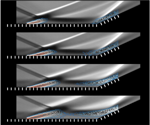
This process can be observed effectively using high-frame-rate schlieren imaging and PIV. The standard deviation of the image intensity obtained from a temporal sequence of $3.2\times 10^5$ schlieren images is illustrated in figure 13, along with the superimposed r.m.s. streamwise velocity fluctuation on the time-averaged schlieren image for case A. Due to the different visual principles on which schlieren imaging and PIV are based, they complement each other in revealing the unsteady features in the interaction region. Schlieren imaging can capture structural changes in flow fields with large density gradients, including shock waves and shear layers. The standard deviation map reveals fluctuations in both the incident shock and boundary layer. However, the magnitudes of these fluctuations are significantly lower than those of the shock oscillation at the compression corner. Within the boundary layer and the interaction region, the PIV enables the quantitative measurement of the flow field, facilitating an accurate assessment of the boundary layer state.

Figure 13.

Fluctuations in the flow field with various spacings between the two STBLI regions in case A. (a) Standard deviation (temporal) intensity maps of the dual-STBLIs obtained from schlieren image sequences. Levels of contour are spaced by 0.2. (b) The r.m.s. streamwise velocity fluctuations normalised by the mean streamwise velocity upstream of the STBLI superimposed with the time-averaged schlieren images. Levels of contour are spaced by 0.02.

When the spacing between the two STBLI regions is relatively large, as depicted in figure 13(a) with $d=52$ and $30\ \text {mm}$, the separation shock becomes distinctly discernible in the standard deviation map. The separation shock manifests as a distinct region characterised by significant intensity fluctuations, indicating the unsteady nature of the STBLI. The downstream boundary layer also exhibits a certain level of turbulence. Shock motions typically arise from specific causes, as evidenced by the PIV results in figure 13(b), indicating a higher level of velocity fluctuation beneath the separation shock within the interaction region. These fluctuations encompass diverse frequencies, including the breathing of the separation bubble and shear layer development. The downstream movement of the incident shock, as illustrated in figure 13 with $d = 30$ and $19\ {\rm mm}$, has a negligible effect on the position of the separation shock at the compression corner. The interaction region at the compression corner is expected to experience an expansion of high-level fluctuations. However, noticeable oscillations of additional waves induced by the UI can be observed distinctly not far upstream in the standard deviation map. The downstream movement of the incident shock leads to a gradual upstream movement of the additional waves generated at the UI, intensifying the oscillations. An analysis of the standard deviation map reveals that variations in the incident shock do not affect the position of the original separation shock at the compression corner. However, violent oscillations are observed in the waves generated at the UI.

The standard deviation map and PIV results enable the observation of amplified oscillations in the upstream influence waves and separation region; however, they do not provide insights into the frequency components present in the interaction regions. To overcome this limitation, we analysed and summarised the SPOD modes across all frequencies. Before further discussions, we would like to emphasise that the number of data samples utilised in this analysis is sufficient. The leading SPOD modal energies obtained with different snapshots of instantaneous fields are shown in figure 14. When the number of snapshots exceeds $1.0\times 10^5$, the difference in energy for low frequencies is minimal, whereas when the number of snapshots exceeds $2.0\times 10^5$, the differences in high frequencies gradually decrease. Considering the very tiny discrepancy between the distributions obtained with $n=2.5\times 10^5$ and $n=3.2\times 10^5$, convergence of the SPOD energy is regarded as sufficient. In addition, the SPOD result exhibits a broadband and energetic low-frequency component associated with the separation shock unsteadiness, which is consistent with the wall pressure measurements.

Figure 14.

Dependence of the SPOD energy convergence on the number of samples.

Three primary shapes emerge, which can be seen in both cases: first, low-frequency oscillations are predominantly influenced by the separation shock; second, medium-frequency oscillations are associated with the oscillation of the separated shear layer; and third, relatively high-frequency oscillations are characterised by small-scale coherent structures originating from vortex shedding. When the two interaction regions are sufficiently far apart, as illustrated in figure 15(a), the typical characteristics of the STBLI can be observed at the compression corner. From the inspection of the leading SPOD mode, we can conclude that the low-frequency oscillations, such as those at $St_{\delta }=0.007$, are dominated by the separation shock motion at the compression corner. This observation is consistent with the fundamental understanding of STBLI, in that separation bubble breathing and large-scale separation shock motion occur predominantly at lower frequencies. The separated shear layer exhibits significant coherent fluctuations, such as flapping of the mixed layer and structural shedding, predominantly at low and medium frequencies ($St_{\delta }=0.007$ and $0.06$).

Figure 15.

First SPOD composed of flow fluctuations obtained from schlieren image sequences in case A with (a) $d=52\ \text {mm}$, (b) $d=19\ \text {mm}$. The plots illustrate low-, medium- and high-frequency oscillations in the flow, arranged from top to bottom. The contours represent the real part of the first SPOD mode, with the levels spaced at intervals of 0.1.

When the two interaction regions are in close proximity, as shown in figure 15(b), an additional shock wave with low-frequency oscillations originates from the UI, and the most energetic fluctuations are in this shock. However, this shock does not exhibit medium- or high-frequency unsteadiness. The shear layer provides energetic contributions at both low and medium frequencies. Similar findings were obtained in a study on the STBLI induced by a compression ramp (Grilli et al. Reference Grilli, Schmid, Hickel and Adams2012). The authors employed dynamic mode decomposition to analyse the presence of a low-frequency mode associated with the pulsation of the separation bubble. In another investigation on transonic STBLI (Sartor et al. Reference Sartor, Mettot, Bur and Sipp2015), Fourier-mode decomposition was utilised to examine the effects of low-frequency perturbations on both the shock wave and the top of the recirculation bubble. At medium frequencies, noticeable elongated coherent structures are present on the compression surface, as depicted in figure 15(b), suggesting intermittent movement of the shear layer in the direction normal to the wall. At a relatively high frequency ($St_{\delta }=0.21$), streamwise periodic structures with small scales appear within the mixing layer in both figures 15(a) and 15(b).

Interestingly, only low-frequency oscillations are observed in the shock waves originating from the UI, which could be due to the existence of the retarded flow in the region upstream from the separation. Murphree et al. (Reference Murphree, Combs, Yu, Dolling and Clemens2021) reported a similar phenomenon, wherein the planar laser scattering and pressure PSD revealed a retarded or weakly separated flow upstream from the region in which the separation was induced by a cylinder. The study conducted by Humble, Scarano & van Oudheusden (Reference Humble, Scarano and van Oudheusden2009) revealed that vortex structures exhibit lifting behaviour even in the absence of a significantly reversed flow region. These vortex structures respond to the highly retarded flow within the inner layer, as illustrated in figure 8, similar to their response to a large-scale recirculating bubble. Consequently, when no substantial deficit exists in the inner layer velocity, no lifting of vortex structures is observed. This finding is particularly important in the present interaction because the upstream STBLI strongly favours the occurrence of retarded flow. Even without a large-scale reversed-flow region, this retarded flow can instantaneously exhibit many features that are typically associated with large-scale separated interactions. In this case, the free-interaction theory provides a mathematical framework for establishing the connection between local conditions and the UI, whereas the presence of retarded flow offers a tangible physical basis.

5.3. Shear layer evolution

The shear layer plays a crucial role in the STBLI. The extent of the separation is determined by the ability of the shear layer originating from the separation point to overcome the pressure increase at the reattachment point. This ability is influenced by the initial momentum available during the process of reattachment. According to the free-interaction theory, it can be observed that the pressure rise leading up to separation is independent of the downstream conditions. Consequently, a higher overall pressure increase applied to the boundary layer or an escalation in shock intensity necessitates a greater pressure increase during reattachment. This increase can be accomplished only by increasing the velocity attained on the dividing streamline; thus extending the length of the shear layer is essential for facilitating more substantial momentum transfer from the outer flow. Additionally, Piponniau et al. (Reference Piponniau, Dussauge, Debieve and Dupont2009) proposed a hypothesis regarding the instability of the STBLI. They suggested that the unsteadiness of the separation bubble could be caused by a process of entrainment and recharge driven by the shear layer. The low-momentum fluid inside the separation bubble can be drawn in by the shedding mechanism through the action of the shear layer. Hereafter, the analysis focuses exclusively on unsteady effects within the separation region.

In case A, the most notable phenomenon is the change in the shock foot. In case B, the oscillation of the separation shock at the upstream position exhibits the expected behaviour, whereas the variation in the shear layer is worth noting. As the two interaction regions gradually approach each other, as depicted in figure 9, reattachment in the upstream region no longer appears, and the shock wave at the compression surface gradually moves downstream with the fusion of the two interaction regions. When focusing on the area between these two regions, many compression waves appear upstream as the spacing decreases.

The standard deviation of the image intensity, along with the superimposed r.m.s. streamwise velocity fluctuation on the time-averaged schlieren image for case B, is depicted in figure 16. When the two interaction regions are far apart, as shown in figure 16(a) with $d=56$ and $45\ \text {mm}$, fluctuations with certain intensities can be observed in the separation and reattachment shocks of the upstream STBLI and the shock wave at the downstream compression ramp. The presence of fluctuations at the edge of the mixing layer originating from vortex shedding, and at the top of the recirculation bubble, should also be considered in the standard deviation map. Similar to case A, regions exhibiting high-level velocity fluctuations are observed within the interaction regions and are situated beneath the separation shocks, as shown in figure 16(b). When the spacing between the two regions decreases, large-range fluctuations caused by compression waves occur between these regions. Simultaneously, the oscillations in the mixing layer between these two regions are enhanced to a certain extent. With an increasing separation scale, the shear layer progressively moves away from the wall. The intriguing aspect lies in the gradual expansion of velocity fluctuation as the two interaction zones approach each other, extending upstream through a separated shear layer. However, the frequency composition of these oscillations remains unknown.

Figure 16.

Fluctuations in the flow field with various spacings between the two STBLI regions in case B. (a) Standard deviation (temporal) intensity maps of the dual-STBLIs obtained from schlieren image sequences. Levels of contour are spaced by 0.2. (b) The r.m.s. streamwise velocity fluctuations normalised by the mean streamwise velocity upstream of the STBLI superimposed with the time-averaged schlieren image. Levels of contour are spaced by 0.02.

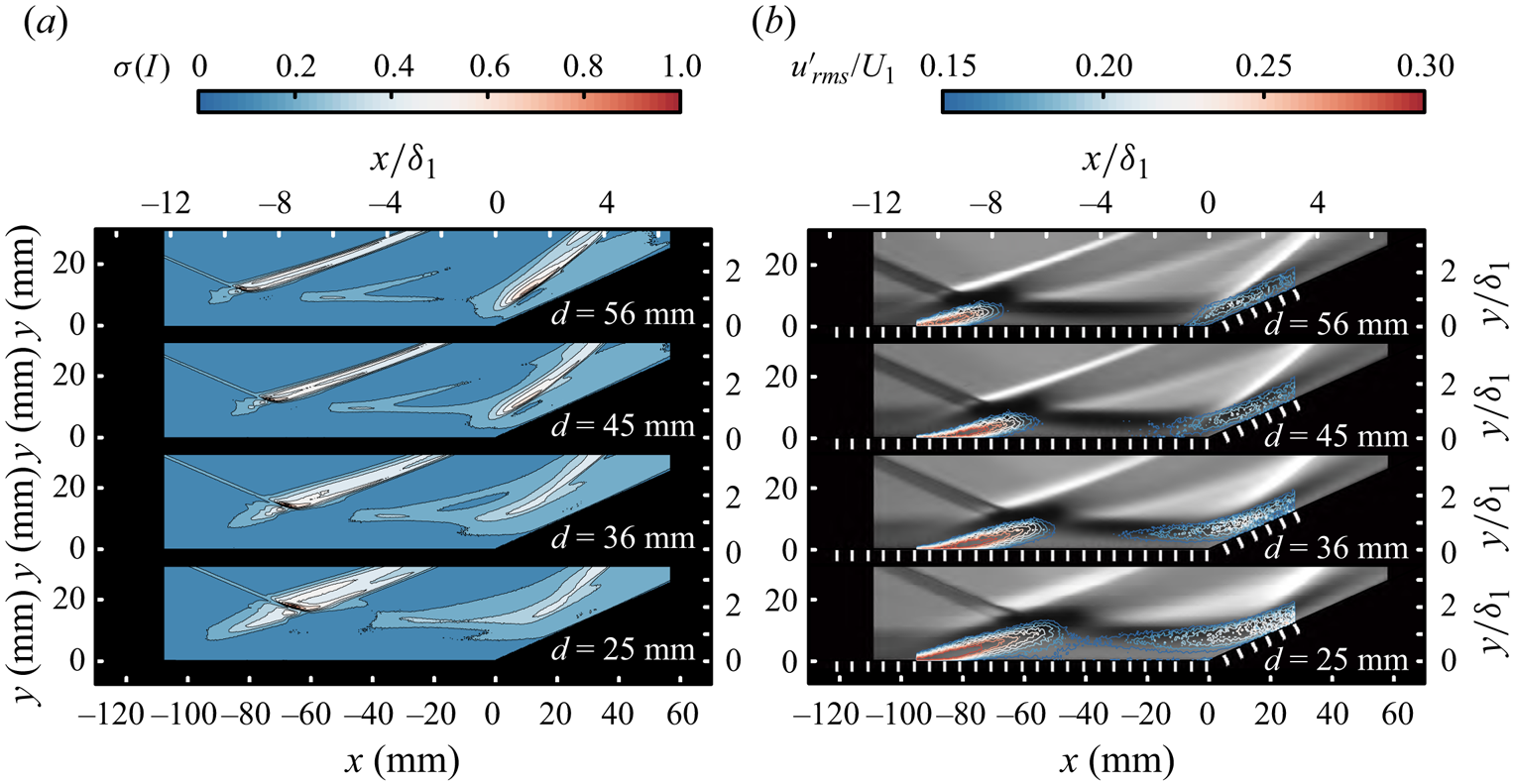
Figure 17 shows the leading SPOD modes of the light intensity fluctuations obtained from the schlieren system. The low-frequency oscillations in all scenarios are governed primarily by the separation shock in the upstream STBLI region, accompanied by the motion of the shear layer normal to the wall, similar to what is depicted in figure 15. Streamwise periodic structures with small scales appear within the mixing layer at high frequencies. When the two interaction regions are widely separated, as depicted in figure 17(a), the range of low- and medium-frequency oscillations in the downstream mixing layer of the first STBLI region is limited, with the perturbation diminishing to a low level at a short distance downstream, whereas high-frequency periodic structures persist until they reach the compression surface. The shock wave at the compression corner is influenced by the mixing layer and vortex structures induced upstream, and these effects can be observed at low, medium and high frequencies. As the two regions approach each other, as shown in figure 17(b), coupled with the observations in figure 9(d), the separation of the mixing layer downstream from the first STBLI region results in more pronounced oscillations that extend to the compression surface, thereby influencing the compression waves above it. The elongated structures within the mixing layer extend continuously to the compression surface, indicating vertical amplitude oscillations of the entire mixing layer. When the scale of separation increases further, the elongated structures move away from the wall with the mixing layer. Notably, both the mixing layer fluctuations and the small-scale eddies originate downstream from the expansion fan or vortex shedding.

Figure 17.

First SPOD mode of flow fluctuations obtained from schlieren image sequences in case B with (a) $d=56\ \text {mm}$, (b) $d=25\ \text {mm}$. The plots illustrate low-, medium- and high-frequency oscillations in the flow, arranged from top to bottom. All plots use the same contour set and spatial coordinates as those in figure 15.

The source of low-frequency oscillations in the STBLI has been summarised in Clemens & Narayanaswamy (Reference Clemens and Narayanaswamy2009) and Souverein et al. (Reference Souverein, Dupont, Debieve, Dussauge, van Oudheusden and Scarano2010). The findings reported in those works indicate the presence of both upstream and downstream effects, with their significance varying depending on the degree of separation and the interaction strength. In cases in which the boundary layer is fully separated, the ‘downstream mechanism’ dominates; however, for mild interactions, the ‘upstream mechanism’ is expected to be more significant. In case B, where the boundary layer is fully separated with an interaction length more than $5\delta _1$ in each scenario, the SPOD analysis results are consistent with the findings of Priebe & Martin (Reference Priebe and Martin2012). The low-frequency oscillation is influenced primarily by downstream effects, with the motion of the shock attributed to the breathing of the separation bubble and the accompanying flapping of the separated shear layer. This is verified further in the cross-correlation analysis that follows.

The enhancement in the low-frequency oscillation between the two regions was analysed further. Taking fixed position T17 as an example, we evaluated the variations in the pressure spectra under different spacings, as illustrated in figure 18. At $d=36\ \text {mm}$, sudden amplification occurs in the low-frequency components, accompanied by a concomitant decrease in the dominant frequency of the high-frequency components. As the incident shock moves downstream, a decrease is observed in the dominant frequency of the high-frequency oscillations, along with slight attenuation in the low-frequency oscillations. The PSD map in figure 11 clearly illustrates that an increase in the separation scale leads to the development of a shear layer originating from the separation point, resulting in lower-frequency fluctuations caused by the Kelvin–Helmholtz instability.

Figure 18.

Frequency-premultiplied PSD of the pressure fluctuations at T17 ($x=-41\ \text {mm}$) with different spacings between the two STBLI regions.

Figure 19 summarises the streamwise development of the characteristic frequency $f_{{ch}}$ during the interaction. The values of $f_{{ch}}$ were obtained directly from the peaks in the spectra at each sensor (refer to figure 11), with approximate uncertainty $5\,\%$. When the two interaction regions are widely separated, such as by $d_{1}=56\ \text {mm}$ (marked by circles) and $d_{2}=45\ \text {mm}$ (marked by squares), $f_{{ch}}$ increases rapidly from the low frequencies at the upstream separation point. It reaches a local peak at approximately $x-x_0=0.2L_{{int}}$ upon shear layer inception, then decreases monotonically along the recirculation region until $x-x_0=0.5L_{{int}}$, where vortex shedding occurs. Subsequently, downstream from the reattachment region, the dominant frequency gradually increases to over $30.0\ \text {kHz}$. This behaviour is consistent with the evolution of the shear-induced disturbances in a typical incident STBLI (Dupont et al. Reference Dupont, Haddad and Debieve2006). The significant disparity is due to the dominant frequency upon inception close to and downstream from the separation; this frequency is $25.8\ \text {kHz}$ in our case, which is more than three times its counterpart observed by Dupont et al. (Reference Dupont, Haddad and Debieve2006) for the incident STBLI ($7.2\ \text {kHz}$). In both cases, this frequency occurs at $x-x_0=0.2L_{{int}}$. Notably, the compression corner study by Thomas et al. (Reference Thomas, Putnam and Chu1994) revealed a dominant frequency of approximately $32.0\ \text {kHz}$ upon shear layer inception, whereas the forward-facing step study by (Chandola, Huang & Estruch-Samper Reference Chandola, Huang and Estruch-Samper2017) yielded a dominant frequency of approximately $37.5\ \text {kHz}$; both of these values are close to the $f_{{ch}}$ value observed here. Notably, a reversal in the trend of $f_{{ch}}$ over the expansion region intrinsic to the incident STBLI case occurs when considering the STBLI in both the forward-facing step (Chandola et al. Reference Chandola, Huang and Estruch-Samper2017) and the compression corner (Thomas et al. Reference Thomas, Putnam and Chu1994).

Figure 19.

Distribution of the dominant frequency $f_{{ch}}$ in the shear layer evolution with different spacings between the two STBLI regions. The two long dashed lines in (a) the schlieren images and (b) the curves indicate the positions at which $f_{{ch}}$ undergoes a reversal and tends to stabilise.

When the two interaction regions approach each other, the schlieren image and pressure distribution reveal an initial separation in the boundary layer downstream from the reattachment, as shown in figure 9(c). Here, $f_{{ch}}$ of the interaction with spacing $d=36\ \text {mm}$, in contrast to those in the previous two scenarios ($d=56$ and $45\ \text {mm}$), experiences a further decrease downstream from the inception of the shear layer, owing to the extended development of the shear layer caused by enhanced separation. Additionally, downstream from the expansion fan, instead of increasing to the high levels observed in the previous two scenarios, $f_{{ch}}$ stabilises at approximately $22.0\ \text {kHz}$. The shift from higher to lower frequencies along the streamwise direction becomes increasingly pronounced as the two regions approach each other, as demonstrated in figure 19 with $d=25$, 16, 6 mm. Subsequently, a gradual increase in $f_{{ch}}$ occurs within the shear layer downstream from the expansion fan, whereas the relatively constant frequencies at the end progressively decrease. In scenarios in which the spacing ranges from $d=36\ \text {mm}$ to $d=6\ \text {mm}$, $f_{{ch}}$ of the shear layer downstream from the expansion fan continues to increase owing to the acceleration of the shed structures induced by the expansion fan. After normalising with respect to the separation length $L_{{int}}$, the results for this region ($0.5L_{{int}}\unicode{x2013}1.2L_{{int}}$) align with the findings reported in the existing literature. When the separation scale is quite large, such as $d=6\ \text {mm}$, $f_{{ch}}$ decreases continuously from the inception of the shear layer. This finding aligns with the trend observed in the compression corner interactions (Thomas et al. Reference Thomas, Putnam and Chu1994), where $f_{{ch}}$ decreases towards a location close ahead of the reattachment. However, contrary to expectations, the previously mentioned acceleration of the shed structures does not result in a significant increase in $f_{{ch}}$, suggesting a weakened effect of the expansion fan.

In addition to changes in $f_{{ch}}$, the evaluation of the energy variations associated primarily with the separation bubble involved integrating the spectra below and above the $1.0\ \text {kHz}$ threshold for further analysis, as illustrated in figure 20. The spectra presented herein were normalised based on the maximum fluctuation energy observed along the plate. Significantly enhanced low-frequency oscillations can be observed near the shock foot, accompanied by high-frequency fluctuations that arise from the shear layer development. The proportion of low-frequency energy compared with the high-frequency component in figure 20(a) is relatively small because of the limited separation scale. However, as depicted in figures 20(b) and 20(c), the approach of the two STBLI regions leads to rapid amplification of the low-frequency energy. However, the subsequent trend demonstrates a gradual decrease in all three scenarios, and a rapid increase at the compression surface.

Figure 20.

Distribution of the spectral energy during the shear layer evolution with (a) $d=56\ \text {mm}$, (b) $d=36\ \text {mm}$, (c) $d=16\ \text {mm}$, at $f< 1\ {\text {kHz}}$ and $f> 1\ {\text {kHz}}$.

As shown in figure 20(a), the high-frequency energy gradually diminishes downstream from the first STBLI region until it reaches the compression corner, where the shock in the second STBLI region leads to a subsequent increase in the high-frequency energy. The enhancement of the separation in figures 20(b) and 20(c) results in a decrease in the dominant frequency, which leads to the amplification of high-frequency fluctuations associated with the shear layer development. The slight decrease in the high-frequency energy followed by a rapid increase near the expansion fan is noteworthy. This inflection point coincides with the reversal of $f_{{ch}}$ at the vortex shedding position, as depicted in figure 19. In these two scenarios, the absence of reattachment in the first STBLI region leads to the continuous development of the shear layer until it reaches the compression corner. This provides favourable conditions for the formation of vortex structures resembling those occurring in the Kelvin–Helmholtz phenomenon within the mixing layer after the separation shock. Scholars have further confirmed that the presence of reverse flow and inflection velocity profiles can result in Kelvin–Helmholtz instability, ultimately leading to the formation of large convective eddies (Dupont et al. Reference Dupont, Piponniau, Sidorenko and Debieve2008; Helm, Martin & Dupont Reference Helm, Martin and Dupont2014).

5.4. Communication within the separation bubble

Ascertaining whether the two interaction regions exhibit coupling at the frequencies of interest is crucial. The coherence function, which quantifies the similarity between wall pressure measurements at different locations within the interaction region, was calculated. The coherence function $C_{xy}$ indicates the level of linearity between signals $x(t)$ and $y(t)$ in terms of the energy content at a specific frequency; $C_{xy}=1.0$ implies a linear relationship between the two time sequences at frequency $f$, whereas $C_{xy}=0$ indicates no correlation.

The coherence function along the streamwise direction in case A is shown in figure 21. The reference transducer used for these coherence functions is positioned at T27, which is close to the origin of the compression corner. Within the incoming boundary layer, $C_{xy}$ maintains a relatively low value that does not exceed 0.2 at any frequency. The highly correlated positions in the separated region surrounding the reference location are shown in figure 21(a), with $C_{xy}>0.4$. Furthermore, the flow at the shock foot is correlated with low-frequency pulsations spanning approximately $10\ \text {mm}$, where $C_{xy}$ exceeds 0.3. Furthermore, as the incident shock moves downstream, $C_{xy}$ at the shock foot increases significantly, reaching maximum value 0.6 in figure 21(b). The range of flow with $C_{xy}$ higher than 0.3 near the shock foot expands to $25\ \text {mm}$, starting from this point. In the initial region of the separated flow, one can observe a narrow passage distinguished by an extremely weak correlation between $x=-11$ and $x=-1$, corresponding to the early growth stage of the shear layer (Murphree et al. Reference Murphree, Combs, Yu, Dolling and Clemens2021; Jenquin, Johnson & Narayanaswamy Reference Jenquin, Johnson and Narayanaswamy2023). Meanwhile, specific high-frequency components, such as $33.1\ \text {kHz}$ in figure 21(a) and $23.5\ \text {kHz}$ in figure 21(b), exhibit a strong correlation with the upstream flow. The regions demonstrating significant values of $C_{xy}$ at these frequencies originate primarily from the initial stage of shear layer development.

Figure 21.

Coherence between the reference signal and the wall pressure at different streamwise locations in case A with (a) $d=52\ \text {mm}$, (b) $d=30\ \text {mm}$, (c) $d=19\ \text {mm}$, (d) $d=10\ \text {mm}$.

The flow associated with the low-frequency oscillations does not extend significantly upstream until the two interaction regions approach each other, as shown in figure 21(c). The flow at sensor T16 demonstrates a noticeable level of correlation, which also implies an expansion of the second STBLI region across the incident shock. The schlieren image reveals that the shock foot at T22 deeply penetrates the boundary layer, indicating the absence of significant separation upstream from the shock foot; however, this region exhibits a lower $C_{xy}$. The region near the shock foot with $C_{xy}>0.3$ remains confined within a span of approximately $25\ \text {mm}$ when the incident shock moves further downstream, as shown in figure 21(d). The superposition of the pressure gradient increases the separation scale at the compression corner, consequently increasing the development length of the shear layer, as evidenced by the extension of the region that is closely related to the high-frequency components. Additionally, a decrease occurs in the dominant frequency of these high-frequency components, from $21.1\ \text {kHz}$ in figure 21(c) to $17.6\ \text {kHz}$ in figure 21(d). This observation is consistent with the evolution trend observed in case B (refer to figure 19) regarding $f_{{ch}}$ of the shear layer, which can be attributed to the elongated development region behind the separation.

The cross-correlation was estimated throughout the measurement domain in order to analyse the temporal organisation of the pressure fluctuations within the interaction region, relative to a reference location situated near the intermittent region and close to the shock foot. The reference location was selected based on the location exhibiting the highest $C_{xy}$ within the intermittent region, as depicted in figure 21. Identifying the STBLI regions that precede or follow the intermittent region is crucial for understanding the underlying mechanisms governing separation shock motion. The presented results are based on an average of 487 selected data snippets, each $2^{14}$ samples $({\approx }30\ \text {ms})$ in length. The presence of a positive (negative) lag at the cross-correlation extremum indicates that the pressure signal at the reference transducer location was lagging (leading). By monitoring the evolution of time delay in the correlation peaks, calculating the average speed and direction of the pressure perturbations was possible. According to figure 21, the signal must be pre-filtered using a low-pass filter at $1\ \text {kHz}$ to eliminate certain complex influences and evaluate the low-frequency effects along the interaction region.

The cross-correlations $\rho _{xy}$ with respect to the signal within the intermittent zone are depicted in figure 22. Similar to the findings depicted in figure 21, the pressure fluctuations in the intermittent region demonstrate a minimal correlation with the incoming boundary layer. The highly correlated area near the reference location is confined. The initial stage of the separated flow near the shock foot exhibits a narrow region in which the correlation is significantly reduced. Downstream, a noticeable negative correlation is observed in the separated flow. This negative correlation persists until reattachment and encompasses the adjacent zones, which is consistent with previous research findings (Priebe & Martin Reference Priebe and Martin2012; Jenquin et al. Reference Jenquin, Johnson and Narayanaswamy2023). In other words, when the pressure in the intermittent zone increases, the pressure inside the separation bubble decreases. This finding indicates that as the separation shock moves upstream, the reattachment point shifts downstream. The periodic expansion and contraction of the separation bubble can be attributed to this combined motion of the separation and reattachment points, which are out of phase. The pressure increases at the location where the separation shock passes, while the upstream pressure of the reattachment shock decreases as it moves rearwards. When the mass is discharged, the internal pressure decreases. In figure 22(a), a maximum positive delay is observed at $x=-11\ \text {mm}$ (T23), which corresponds to the shock foot identified in figure 5(a). Furthermore, the pressure variation at this location precedes values at the other locations, indicating the origin of the disturbance. Based on the spacing between the transducers, the average velocities of the upstream- and downstream-propagating disturbances can be calculated as $0.37u_{\infty }$ and $0.42u_{\infty }$, respectively. As the incident shock moves downstream, the cross-correlation distributions in figures 22(b) and 22(c) exhibit similarities to the previous ones. With a slight enhancement in the separation scale, the propagating velocities decrease. When the incident shock enters the interaction region, it amplifies the oscillation of the shock at the UI, increasing the upstream-propagating velocity, as depicted in figure 22(c). However, as the separation scale increases, larger vortex structures decrease the downstream-propagating velocity as illustrated in figures 22(c) and 22(d). A second peak of delay within the separation region becomes increasingly prominent as the separation scale increases, as depicted in figures 22(c) and 22(d). Both upstream- and downstream-propagating disturbances can also be observed to originate at this location.

Figure 22.

Streamwise evolution of the two-point cross-correlations of different zones within the STBLI region with reference to the intermittent region in case A with (a) $d=52\ \text {mm}$, (b) $d=30\ \text {mm}$, (c) $d=19\ \text {mm}$, (d) $d=10\ \text {mm}$.

Although the linear coupling between the pressure at the shock foot located at the compression corner and the pressure fluctuations in the upstream boundary layer is relatively weak, as demonstrated in figures 21 and 22, this finding is consistent with those of previous studies, which have indicated a weak correlation between the low-frequency mode of the STBLI and the incoming boundary layer (Piponniau et al. Reference Piponniau, Dussauge, Debieve and Dupont2009; Huang & Estruch-Samper Reference Huang and Estruch-Samper2018). However, this does not diminish the effects of the upstream boundary layer conditions on the STBLI. A boundary layer with a full profile reduces the separation tendency, whereas an incomplete profile renders separation more likely. In numerous studies (Kim & Adrian Reference Kim and Adrian1999; Adrian, Meinhart & Tomkins Reference Adrian, Meinhart and Tomkins2000; Ganapathisubramani, Clemens & Dolling Reference Ganapathisubramani, Clemens and Dolling2007; Humble, Scarano & van Oudheusden Reference Humble, Scarano and van Oudheusden2007; Jenquin et al. Reference Jenquin, Johnson and Narayanaswamy2023), a strong correlation has been observed between the fluctuations in the upstream velocity and the separation location. The presence of elongated low-speed structures within the upstream boundary layer aligns with the occurrence of separated flow. These disturbances in the boundary layer induce shock motion, leading to pressure fluctuations at the shock foot that precede those observed at other locations within the separation bubble. This phenomenon is demonstrated clearly in figure 22, where pressure fluctuations at the shock foot are observed prior to those inside the separation bubble or at the reattachment point in all six scenarios. The lag of the pressure fluctuations within the upstream boundary layer with respect to the reference location is illustrated in figure 23. Even though the correlation coefficient is low, not exceeding 0.2, a constant velocity close to $0.1U_{1}$ can be detected, implying the downstream propagation of larger-scale, low-speed structures. The origin of this disturbance is located precisely downstream from the incident shock in the first STBLI region, as evidenced by its identical displacement when the incident shock wave moves downstream by $10\ \text {mm}$. Tracing back further reveals that the ultimate source lies within the boundary layer at an even more upstream position, where the disturbance with propagation speed $0.51U_{1}$ originates, and continues to propagate downstream after deceleration through the first interaction zone.

Figure 23.

Two-point cross-correlations of different regions within the incoming boundary layer with reference to the intermittent region in case A with (a) $d=52\ \text {mm}$, (b) $d=41\ \text {mm}$.

In case B, when the two interaction regions are widely separated, the flows at the compression corner and the reference location are strongly correlated, as shown in figure 24(a). Additionally, at frequencies below $2.0\ \text {kHz}$, a correlation exists between the shock oscillation at the compression corner and the nearby upstream flow. Furthermore, a relationship is evident between the separation shock in the first STBLI region and the interaction region at the compression corner; however, these correlations are relatively weak and do not exceed 0.3. No discernible correlation is observed in terms of flow between these two regions with respect to the reference position. The reduction in the spacing between the two interaction regions, as illustrated in figure 24(b), leads to a similar observation for the correlation in the high-frequency components compared to that in case A. In figure 24(c), a significant change is observed in the correlation between the flow at the compression corner and the upstream interaction region. Initially, the changes in the properties near the reference position are negligible; however, a noticeable increase occurs in the correlation coefficient between the reference position and the low-frequency oscillations induced by the upstream separation shock. Furthermore, a higher level of correlation is observed in the region between the separation shock and the compression corner. Finally, significant upstream expansion occurs in the area that is highly correlated with the high-frequency component centred around $22.0\ \text {kHz}$ at the reference position. The origin of this region coincides with the location at which vortex shedding occurs in the upstream STBLI, which also corresponds to the location of the reversal in $f_{{ch}}$ from a lower to a higher level, as shown in figure 19.

Figure 24.

Coherence between the reference signal and the wall pressure at different streamwise locations in case B with (a) $d=56\ \text {mm}$, (b) $d=45\ \text {mm}$, (c) $d=36\ \text {mm}$, (d) $d=25\ \text {mm}$.

In the subsequent scenarios, a clear separation is evident in the boundary layer between the two interaction regions, and a similar correlation distribution is observed. As the incident shock moves downstream, the dominant frequency of the highly correlated high-frequency components gradually decreases, which aligns with the results in figure 19. These highly correlated high-frequency fluctuations are attributed solely to unsteady shear layer flow. This observation confirms the coupling between the downstream pressure fluctuations and the low-frequency motion of the separation shocks as well as the high-frequency unsteady flow in the shear layer, enhancing our understanding of their interactions.

When the two interaction regions are far apart, as shown in figures 25(a) and 25(b), less of a correlation exists between the downstream flow and upstream separation shock, which aligns with the results in figure 23. A negative peak with positive maximum delay $0.082\ \text {ms}$ occurs at T11 in the separation region, as shown in figure 25(a). The time delay decreases with increasing upstream distance, indicating an upstream-propagating perturbation, whereas the time delay increases with increasing downstream distance, suggesting a downstream-propagating perturbation. Both the upstream- and downstream-propagating disturbances originate at this location, which is consistent with the findings for shock-induced separated flows, where large structures that develop in the mixing layer occur near the middle of the bubble ($x-x_0= 0.5L_{{int}}$) (Dupont et al. Reference Dupont, Haddad and Debieve2006). Downstream from the first interaction region, the disturbance propagates at velocity $0.67U_{1}$. Although the fluctuations downstream from the interaction region exhibit certain delays relative to those in the upstream separation region, the correlation remains weak and does not exceed 0.3. In the subsequent scenarios, as the separation scale increases, the magnitude of the eddies evolving along the shear layer also increases. Following vortex shedding, larger-scale eddies propagate downstream at a reduced velocity.

Figure 25.

Streamwise evolution of the two-point cross-correlation of different regions within the STBLI zone with reference to the intermittent region in case B with (a) $d=56\ \text {mm}$, (b) $d=45\ \text {mm}$, (c) $d=36\ \text {mm}$, (d) $d=25\ \text {mm}$.

Similar to case A, the fluctuations are approximately in phase in the region surrounding the separation location; however, a phase shift ${\rm \pi}$ exists within the separated flow. This finding aligns with the experimental results observed in the case of a reflected shock (refer to Dupont et al. Reference Dupont, Haddad and Debieve2006; Debieve & Dupont Reference Debieve and Dupont2009; Touber & Sandham Reference Touber and Sandham2009). Jenquin et al. (Reference Jenquin, Johnson and Narayanaswamy2023) also reported a phase shift ${\rm \pi}$ in wall pressure during the compression-ramp-induced STBLI. In summary, previous research indicates that regardless of the type of shock boundary layer interference, this phase alteration remains consistent and is associated with the expansion/contraction of the separation bubble. The pressure changes within the bubble, particularly at the vortex shedding location, occur before those at the other locations in the six scenarios considered. This finding is consistent with the shear layer entrainment–recharge mechanism proposed in numerous studies.