


Introduction
Recently, there has been increasing interest in sex-specific effects of developmental programming.Reference Dunn, Morgan and Bale 1 , Reference Aiken and Ozanne 2 Literature searches on PubMed and Web of Science from 2000 to 2014 show that there has been a substantial increase in studies examining sex-specific effects of developmental programming – searches for the terms ‘sex-specific or sex-dependent’ and ‘fetal or development’ and ‘programming’ yielded only 14 studies published in 2000 and 84 studies published in 2014. Differential susceptibility to developmental programming between the sexes has been demonstrated widely in animal models.Reference Aiken and Ozanne 2 Moreover, funding agencies such as National Institutes of Health and Canadian Institutes for Health Research are increasingly encouraging the incorporation of gender and sex into research designs where appropriate.
In assessing whether effects are sex-specific, it is necessary to explicitly test whether an effect differs between the sexes; performing analyses separately for each sex is not sufficient. For example, if the effect of treatment is significantly different from zero in males, but not in females, it does not necessarily follow that the effect size in males is significantly different from the effect size in females. A non-significant effect in females is not evidence that the effect size in females is actually zero. Conversely, if the effect of treatment is significant and in the same direction in both sexes, it does not necessarily follow that the magnitude of the effect of treatment is equal in both sexes. We argue that, in order to report an effect as ‘sex-specific’ or ‘sex-dependent’, it is necessary to perform an explicit test of the difference in effect size between the sexes, for example, using a sex by treatment interaction term in the statistical model. We examined the reporting of statistical models in experiments that reported sex-specific effects of developmental programming, and whether an explicit statistical test of differences in effect between the sexes was described.
Methods
Papers
We searched the ISI Web of Knowledge (http://www.isiwebofknowledge.com) and PubMed (http://www.ncbi.nlm.nih.gov/pubmed) databases for papers published in 2012 through 2014, using a combination of the search terms ‘sex-specific or sex-dependent’, ‘fetal or development or gestational’, and ‘programming’. To be included in our survey, studies had to involve a maternal treatment during pregnancy, followed by a measurement of offspring physiology. We assessed whether the authors performed an explicit statistical test of differences in effect between the sexes, for example, a sex by treatment interaction term.
Results
In total, there were 34 rodent studies that met the search criteria from 2012 to 2014, and of these, 31 reported sex-specific effects. Only 11 studies reported a sex by treatment interaction, utilizing general linear models (e.g. ANOVAs), while the remaining 20 studies analyzed the sexes separately. Studies that analyzed the sexes separately utilized Student’s t-tests, Mann–Whitney U tests, and ANOVAs. All nine studies of other organisms, including sheep, pigs and baboons, reported sex-specific effects. However, only three studies reported a sex by treatment interaction term, utilizing general linear models (e.g. ANOVAs) while the others analyzed the sexes separately using ANOVAs.
Discussion
Only a third of studies reporting sex differences in developmental programming effects included a sex by treatment interaction term in their statistical models. Instead the sexes were analyzed separately, and significant effects detected in only one sex were described as sex-specific. However, this is not a robust approach, and studies in developmental programming should include explicit statistical tests for sex-specific effects, for example, by including interaction terms between sex and treatment.
While small sample sizes may limit the statistical power to detect interactions, this is not a justification for excluding explicit statistical tests for sex-specific effects. Where the sex by treatment interaction term is not significant, an alternative approach would be to report confidence intervals for the magnitude of effect in each sex. While confidence intervals would overlap between the sexes if the interaction was not significant, this approach would illustrate the potential magnitude of differences between the sexes.
Another alternative approach would be the use of Bayesian analysis. Traditional null hypothesis significant testing (NHST) uses P-values, which describe the probability of observing the test statistic or one more extreme if the null hypothesis is true (e.g. there is no effect of treatment). In contrast, Bayesian analysis quantifies degree of belief or uncertainty in a parameter or hypothesis using probability distributions.Reference Wagenmakers 3 Thus, while NHST calculates the probability of observing the test statistic or one more extreme, given some null hypothesis, Bayesian approaches calculate the probability of some hypothesis or parameter value, given the data.Reference Stephens, Buskirk and Martínez del Rio 4 Therefore, Bayesian approaches actually allow more intuitive statements to be made than does NHST. While Bayesian approaches provide the opportunity to incorporate prior knowledge into analyses, it is possible to use prior distributions that are uninformative, that is, that have little impact on the results.Reference Wagenmakers 3 Bayesian analysis begins with a prior probability distribution (e.g. for parameter values) and uses the prior and sample data to produce a posterior distribution, from which one can determine the probability of some parameter value, given the dataReference Eddy 5 (see Appendix 1 for more detail).
In the Appendix, we provide an example of a Bayesian approach to express the level of confidence that effect size differs between males and females, using both SAS and an open-source package available for R. 6 Instead of focusing on whether or not the difference in effect size between males and females is statistically significant (i.e. different from zero), this approach quantifies the degree of confidence that this difference is sufficiently large to be biologically interesting, which is arguably a more important issue. Our example illustrates the flexibility of Bayesian analysis, which allows one to calculate the probability of a customized parameter value or hypothesis. Furthermore, while Bayesian approaches may currently be unfamiliar to many biologists and clinicians, the analyses that we have described are very easy to implement. This approach provides probabilities that are straightforward to interpret, but does not provide a clear-cut, ‘significant or not’ answer in the way that a P-value might. However, NHST does not necessarily provide less ambiguous results, for example, a non-significant P-value does not provide evidence that an effect does not exist, and conversely a significant P-value does not necessarily indicate that an effect is biologically important. Furthermore, because NHST reduces the results to a dichotomy (significant or not), with small sample sizes one is more likely accept the null hypothesis even if it is false, that is, commit a type II error. With small sample sizes, there will be more uncertainty in Bayesian estimates,Reference Kruschke 7 but there will not be a greater chance of error. Therefore, even if sample size limits the statistical power to detect a sex by treatment interaction term, Bayesian approaches allow researchers in developmental programming to assess the probability of sex-specific effects.
Acknowledgments
The authors thank Richard Morey, Tim Swartz and Ian Bercovitz for advice regarding the interpretation of Bayesian analyses and William Tian for help with the literature search.
Appendix 1. Example of a Bayesian approach to express the level of confidence that effect size differs between males and females
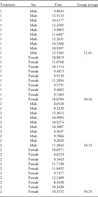
To illustrate a Bayesian approach, we have simulated a data set where a trait has been measured in male and female individuals subjected to one of two treatments (Table A1). When analyzing the sexes separately using a one-way ANOVA, there is a significant effect of treatment on the trait in males (F 1,18=5.19; P=0.04), but not in females (F 1,18=0.03; P=0.86). However, when analyzing the sexes together using a two-way ANOVA and including a sex by treatment interaction term, the interaction is marginally non-significant (F 1,36=3.46; P=0.07). This is a situation in which many authors would be inclined to report sex-specific effects, and yet we have argued that sex-specific effects should not be reported unless there is a significant sex by treatment interaction term. A Bayesian analysis provides an alternative way to express the level of confidence that effect size differs between males and females.
Simulated data set

Before considering a Bayesian approach, it is necessary to consider what is tested by including a sex by treatment interaction term in a model, that is, whether the effect of treatment differs between the sexes. If there are only two treatments, the sex by treatment interaction can be quantified by a single number: the difference in effect size between males and females, and the P-value for the interaction tests whether this number is significantly different from zero. In our example, the effect size in males is (11.41–10.13)=1.28, whereas it is (10.16–10.25)=−0.09 in females. Thus, the difference in effect sizes is −0.09–1.28=−1.37 (note that this value could also be calculated as 1.37, depending on which means are subtracted from which). While such estimates of the magnitude of an interaction are often not reported, it is useful to consider this estimate and whether a difference in effect size is biologically important, rather than simply whether or not a difference is statistically significant from zero.
We performed Bayesian analyses using a BAYES statement in proc GENMOD in SAS ver. 9.3 (see Appendix 2 for code), and using the BayesFactor package version 0.9.11-1 in R (see Appendix 3 for code). To interpret the results of a Bayesian analysis, it is necessary to understand the posterior distribution. The analysis uses random simulation to approximate the posterior distribution by generating many (e.g. 10,000) combinations of parameter values that are consistent with the observed data and the prior distribution (although an uninformative prior can be selected which will have little influence on the results).Reference Kruschke 7 In this case, the parameters include the effects of sex, treatment and the sex by treatment interaction, and each combination of parameters generated by the analysis is a posterior sample.
One of the results of the SAS analysis is an estimate of the sex by treatment interaction, that is, –1.37, as calculated above; this parameter is not calculated automatically by BayesFactor, but can be obtained from its output (see Appendix 3). Another result of the SAS analysis is the 75th percentile of the sex by treatment interaction among posterior samples, which is −0.86 (Table A2). In other words, the sex by treatment interaction is less than −0.86 in 75% of posterior samples. Thus, one could report that there is a probability of 0.75 that the difference in effect size between males and females is 0.86 or greater. If 0.86 was considered a biologically important difference, one could conclude that there was a substantial probability (0.75) that the difference in effect between males and females was biologically important. Note that the Bayesian approach allows a more intuitive statement than that one would obtain from a traditional confidence interval (e.g. ‘were we to repeat the experiment many times, the 95% confidence interval would include the true value in 95% of repetitions’).
What if 0.86 was not considered a biologically important difference? One could alternatively identify a different value for the sex by treatment interaction, and determine its probability. This can be achieved quite easily using the distribution of the sex by treatment interaction among posterior samples (which can be obtained using the OUTPOST option in the BAYES statement in SAS, or the POSTERIOR function in BayesFactor). For instance, if a difference in effect size of 1.2 would be considered biologically important, one can determine where 1.2 occurs among the set of posterior samples. In this example, among 10,000 posterior samples, the 5836th lowest value is −1.20054 and the 5837th lowest value is −1.19970 (values will vary slightly from run to run because the algorithm used by the analysis involves random simulation). Thus, one could conclude that ‘there is a probability of 0.58 (5836/10,000) that the effect size in males is at least 1.2 units greater than that in females’ (Table A2). Such a statement might not provide very convincing support for the existence of a sex-specific effect. However, this statement has incorporated consideration of what is or is not a biologically important difference, in contrast to the observation that the effect is significant in one sex, but not in the other. The selection of a ‘biologically important’ effect size could be achieved objectively, for example, by using an effect size observed in a seminal paper in the field, or an effect that would be considered clinically important in humans.
Discussing the difference in effect size in absolute terms will not be very intuitive in many cases. There might be a variety of other thresholds to determine whether the difference in effect size between males and females is biologically important. For instance, it might be meaningful to express the difference in effect size as a percentage, for example, what is the probability that the difference in effect size between males and females is at least 10% of the value in control males? This is possible using the posterior samples from a Bayesian analysis by (1) calculating the difference in effect size between males and females for each posterior sample, (2) calculating the mean value for control males in each posterior sample, (3) assessing whether the difference in effect size is greater than 10% of the mean of control males in each posterior sample, and (4) counting the proportion of posterior samples for which this condition is true, that is, the posterior probability that the difference in effect size between males and females is at least 10% of the mean value in control males, which in this example is 0.62 (Table A2). Again, this is not convincing evidence of a sex-specific effect, but unlike traditional NHST, this approach has assessed the evidence of a biologically important sex-specific effect. Thus, this approach provides a more meaningful interpretation of the data than the traditional approach described at the beginning of this example, that is, one way ANOVAs performed separately for each sex, without a sex by treatment interaction term.
Comparison of results between SAS and R (see Appendices 2 and 3 for details)

Appendix 2. SAS code
* treat refers to treatment, which can be 1 or 2;
* sex is coded as M or F;
proc genmod;
class treat sex;model trait=treat|sex/type3;lsmeans treat*sex;
* The code below is the default analysis, which uses a noninformative uniform prior;
* The "outpost" option creates a dataset (named "post") containing the posterior samples;
bayes outpost=post;
* this is an alternative, which specifies the use of a Jeffreys" noninformative prior;
bayes COEFFPRIOR=JEFFREYS outpost=post;
* In the dataset containing the posterior samples, SAS creates a variable "treat1sexf", which is the estimate of the difference in effect size between males and females;
* The dataset is sorted by treat1sexf to determine, e.g., where a difference of 1.2 ranks among posterior samples;
proc sort data=post;
by treat1sexf;
proc print;
* For each posterior sample, the estimate for each of the four groups (i.e., treatment 1 males, treatment 1 females, etc.) can be calculated;
* The way SAS estimates the parameters is that one group mean is set as the intercept, and then effects of treatment, sex and treatment*sex are estimated as deviations from that reference group;
* In this example, the parameter "treat1" describes the effect of treatment 1 compared to treatment 2, the parameter "sexf" describes the effect of being female compared to being male, and the parameter "treat1sexf" describes the deviation of the mean of the treatment 1 females from what would be expected given the effects of treatment and sex;
data post;
set post;trt1sexf=intercept+treat1+sexf+treat1sexf;trt1sexm=intercept+treat1;trt2sexf=intercept+sexf;trt2sexm=intercept;
* Once the means of each of the four groups are calculated, it is possible to calculate customized parameters, e.g., whether the difference in effect size is greater than 10% of the mean of treatment 1 males in each posterior sample;
ratio=0.1*trt1sexm;
* abs(treat1sexf) returns the absolute value of the difference in effect size between the sexes for each posterior sample;
if abs(treat1sexf)>ratio then check=1; else check=0;
* The variable "check" allows the calculation of the proportion of posterior samples in which the difference in effect size between males and females is at least 10% of the value in treatment 1 males;
proc freq;
tables check;
Appendix 3. R code
# load the "BayesFactor" package
library(BayesFactor)
# The following command computes the Bayes Factor for a linear model (hence "lmBF")
# The model is the full model, i.e., treatment, sex, and interaction term
# "full" is the name of the object containing the results – a another name could be used instead
# "rscaleFixed" is the prior scale, which is set to a large number to avoid shrinkage
# Shrinkage isn't necessarily undesirable, however, avoiding shrinkage is necessary to make the results comparable with those from the SAS analysis described in Appendix 2
# For a discussion of shrinkage, see Kruschke (2013)
full <- lmBF(trait ~ treat+sex+treat:sex, data=sextreatint, rscaleFixed=100)
# The "posterior" function samples from the posterior distribution
# BayesFactor calculates the parameters differently than SAS (Appendix 2)
# In this example, parameters include
# the grand mean
# a female effect and a male effect(equal in magnitude to the female effect, but in the opposite direction)
# an effect of treatment 1 and an effect of treatment 2 (equal in magnitude to the effect of treatment 1, but in the opposite direction)
# four estimates of treatment by sex interaction effects (i.e., one for each group)
chainsfull <- posterior(full, iterations=10000)
# Those adept at the R language could perform calculations using the posterior distribution directly in R
# Alternatively, the posterior samples can be written to an Excel file for analysis using different software
# Load the "xlsx" package - this is needed to write the posterior samples to an Excel file
library(xlsx)
# Write the posterior samples to an Excel file (be patient)
write.xlsx(chainsfull,"BayesFactor_posteriors.xlsx")