I. INTRODUCTION
The instrumented indentation test (IIT) is getting popular as a material test, which can evaluate not only hardness but other material parameters such as elastic modulus or viscosity. IIT with shallower indentation than 1 μm is called nanoindentation and particularly demanded to evaluate multilayered semiconductor devices, hard coating on optical discs or machining tools, etc. Due to the expanding usage of this technique, the confirmation of the reliability of IIT is becoming important. It depends on the calibration of testing machines. As the ISO (International Organization for Standardization) standards1 are requiring, it shall be done by the both of direct and indirect methods.
The direct method is the procedure of the calibration and verification of every machine element including testing force, depth measuring device, testing cycle, etc. In addition, the indenter geometry (or the area function) and the frame compliance are important items especially for nanorange IIT. The reason is that in nanorange only the small part of the tip of indenter is pressed into the sample, but in general, it is difficult to keep the indenter tip in exact geometry in such a small area due to the limitation of manufacturing technique. In addition, the deformation of the frame is not negligible because the penetration depth itself is small. The practical calibration method of the area function, i.e., the relation between contact depth and contact area of indenter, and the frame compliance was proposed by Oliver and Pharr.Reference Oliver and Pharr2 With this method, both of the area function and the frame compliance are determined through a series of indentation tests with various penetration depths at the same time. Their method is widely accepted in practice because of its usability, but the efforts to improve the reliability of calibration result are still being made by other reseachers.Reference Ishibashi, Ohki, Takagi, Yoshikawa, Katayama, Iwatsubo and Fujitsuka3 For this purpose, the atomic force microscope (AFM) can be a powerful tool.
The AFM is getting popular to observe objects in extremely high magnification. In addition, closed-loop controlled AFM, so called as “metrology AFM,” is recently used to evaluate the geometry of an object, not only in nanoscale but microscale, and now it becomes one of the necessary tools to establish the standards of micro- to nanorange IIT.
One usage of AFM for IIT standard is the direct verification of indenter,Reference Hasche, Herrmann, Pohlenz and Thiele4–Reference Fischer-Cripps7 which includes the verification of the indenter tip and the evaluation of the area function. Directly measured area function with an AFM is more reliable than that evaluated by any other indirect method, and it helps us obtain reliable values of hardness.
Another usage of AFM is the characterization of the reference standards (certified reference materials [CRMs]). For the calibration of the frame compliance or the indirect verification of the testing machine, well-studied reference materials are needed. To perform the verification and calibration of testing machines in a wider range of hardness or elastic modulus, many kinds of CRMs are desirable. But the deformation of the materials is different according to their mechanical properties, and it is not easy to determine the certified values of them. It is expected to improve the reliability of calibration values of CRMs through the direct observation of the indents by an AFM and the analyses of geometry of those indents.
In this article, observed images of indenters are demonstrated with their geometrical analyses by the methods which are developed previously by authorsReference Takagi, Usuda, Kongkavitool and Ishibashi6, Reference Takagi, Hattori, Seino and Nakano8, Reference Takagi and Ishibashi9 and the uncertainty of measurement is discussed. In addition, observed images of indents are also demonstrated as an example of the characterization of CRMs. Through those applications, the availability of AFM is shown in the point of view of the measurement standard.
II. INDENTER VERIFICATION WITH AN AFM
The AFM Nano-R manufactured by Pacific Nanotechnology, Inc. (Santa Clara, CA) was used for this study. This instrument is equipped with a closed-loop control system to compensate creep behaviors of the piezoelectric translator of its scanner with position sensors attached on it. With this system, it achieves better than 1% of linearity. The resolutions of x- and y-directions are <2 nm (with closed-loop control) and the noise level in z-direction is <0.13 nm. The maximum travel of the scanner is 80 μm in x- and y-directions and ±8 μm in z-direction.10 Therefore the working distance of this AFM covers nano- to microrange of the indentation.
An example of obtained AFM image of a Vickers indenter used for PICODENTER HM500 nano-hardness tester (Helmut Fischer GmbH, Sindelfingen, Germany) is shown in Fig. 1. The size of this image is 4.8 × 4.8 μm2 and it was scanned with the resolution of 256 pixels × 256 pixels. This image size is determined empirically for the verification of the pyramidal part and the point of indenters at the same time. From this size of image, the geometry within approximately 500 to 600 nm in penetration depth can be verified.
Atomic force microscope (AFM) image of a Vickers indenter in the field of view of 4.8 × 4.8 μm2.

III. INDENTER GEOMETRY OF PYRAMIDAL PART
For relatively deeper indentation, the indenter geometry of pyramidal part plays an important role to determine the hardness value. To verify the indenter geometry, facet angles of three or four faces (Berkovich or Vickers indenter, respectively) should be evaluated, as well as the area function calibration.
Usually the geometry of AFM images is analyzed with the built-in software of each AFM. This method, however, cannot be used to precise evaluation because of following reasons.
One reason is that the manipulation with a graphical user interface (GUI) and an operator’s hand does not have enough accuracy. Even though ISO standard requires ±0.3° of accuracy for the facet angle and the interior angle of the base of pyramid, evaluated values can vary more than this by human factor during analysis process.
Another reason is that the axis of indenter pyramid is not always identical to the axis of AFM. This misalignment also affects the evaluated angles but even so the built-in software of AFM cannot correct the inclination of axis.
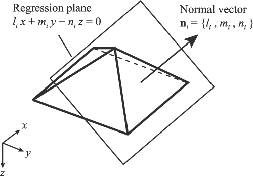
To avoid these problems, authors proposed fully mathematical method to evaluate the indenter geometry, which is named as the Regression Polyhedral Model.Reference Takagi, Usuda, Kongkavitool and Ishibashi6, Reference Takagi, Hattori, Seino and Nakano8, Reference Takagi and Ishibashi9 In this method, AFM image (bitmap data) is divided into three or four groups along the edge of pyramid so that only pixels of each face are contained in each group. Then, each pixel group is fit to the regression plane by the least square method. Now, the bitmap data is translated into a model of the analytical geometry as

in Hesse normal form or

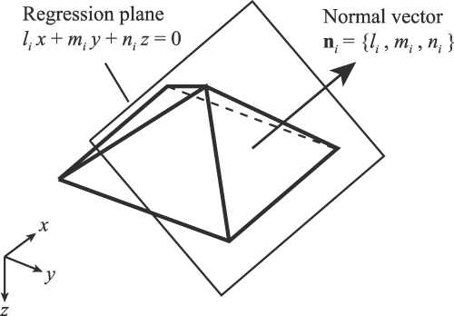
which express z as the function of x and y, where li, mi, ni, pi,  , bi, and ci are the constants determined through the regression analysis, and the suffix i is the identification of the face of pyramid. The direction of each face can be expressed by its normal vector

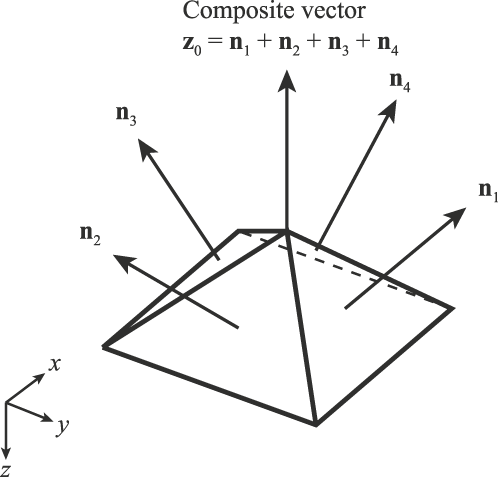
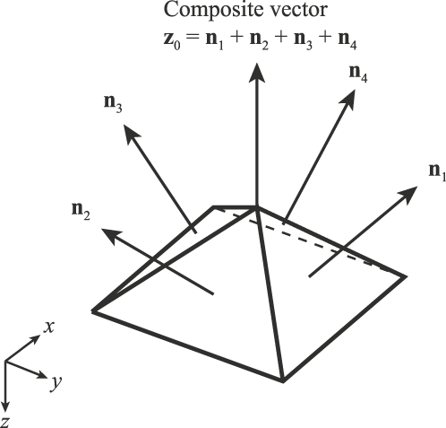
as shown in Fig. 2. Before the geometry of this mathematical model is analyzed, the inclination of the axis (z-axis) should be determined to correct the model alignment. In this study, the axis of the pyramid is defined as the composite vector of the normal vectors of all faces

Regression analysis of a face of pyramid.
as shown in Fig. 3.
Definition of the axis of pyramid.
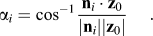
Facet angles of pyramid can be derived using the inner product of ni and z0 as
The angle between opposite faces of Vickers indenter and the interior angles of the base of pyramid can also be derived in the same way. It should be noted that the evaluation process of these angles are fully mathematical and never include human factors.
The uncertainty of every regression plane, which comes from the flatness and the roughness of the face of an observed image, and instrument noise is estimated from the root mean square error,
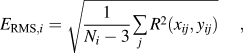
where R(xij,yij) is the residual of the regression plane from the observed image at the coordinates of (xij, yij), and  is the identification of the pixel contained in the face i.
Based on E RMS,i, the standard uncertainty of the constants in the equation of the regression plane [Eq. (2)] can be derived as follows:



In addition, the standard uncertainty of the normal vectors can be expressed as

where Cij is the coefficients of the root of Gauss’ normal equation in the regression analysis,

and defined as

where  represents the summation with respect to j.
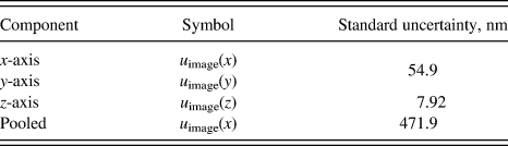
The uncertainty of evaluated angles can be calculated with the uncertainty of the normal vectors [Eq. (10)] by considering the propagation of errors. The first step of the uncertainty estimation is estimating the uncertainty of the AFM. It can be achieved by combining resolution and linearity of the AFM, the effect of the scanning tip, and the uncertainty of the reference standard used to calibrate the AFM. Estimated uncertainty of the AFM is now denoted as u image (x), u image (y), and u image (z) for x-, y-, and z-axes, respectively. Since the slope of Vickers indenter is gentle (only 22° from xy plane) and the uncertainty components in x- and y-direction seem not to cause significant effect on angle calculation, it is convenient to pool u image (x) and u image (y) into u image (z) and express all uncertainties in single number as

for the further (the third) step of uncertainty estimation.
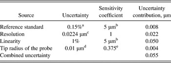
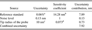
Estimated uncertainty of the AFM is shown in Tables I(a)–I(c).
Estimated uncertainty of the x- and y-axes of the atomic force microscope (AFM).

a 0.03 μm for 10 μm (k = 2).
b Scanning size for the indenter verification.
c Assumption of the rectangular distribution in the scanning interval of 5 μm image with the resolution of 256.
d Typical value described in the manufacture’s catalog (Nanosensors).
e Maximum error in x- or y-direction when the slope of 22° is measured.
Estimated uncertainty of the z-axis of the AFM.

a 2 nm for 181.1 μm (k = 2).
b Pyramid height for the scanning area of 5 μm.
c Typical value described in the manufacture’s catalog (Nanosensors).
d Maximum error in z-direction when the slope of 22° is measured.
The uncertainty of coordinates of the AFM can be estimated by combining the contributions of the reference standard (VLSI STS3-1800P), the resolution (or the maximum noise level) of the image, the linearity of the scanner, and the tip radius of the probe. Therefore the uncertainty of AFM coordinates measurement can be summarized as Table I(c).
Summary of the estimated uncertainty of the AFM.
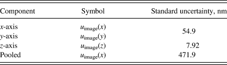
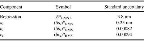
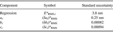
The second step of uncertainty estimation is the evaluation of the regression error. As previously described, it can be carried out with the root mean square error E RMS,i. An example of the uncertainty estimation of the regression is shown in Table II.
An example of the uncertainty estimation of a regression plane.
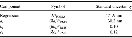
The third step of uncertainty estimation is combining the uncertainty of AFM and the regression. It can be carried out as follows:


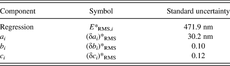
An example of the combined uncertainty is shown in Table III.
An example of the combined uncertainty of the regression plane.
Then the standard uncertainty of facet angle αsfor face s and the interior angle of the base of pyramid θrs between faces r and s can be estimated as follows:


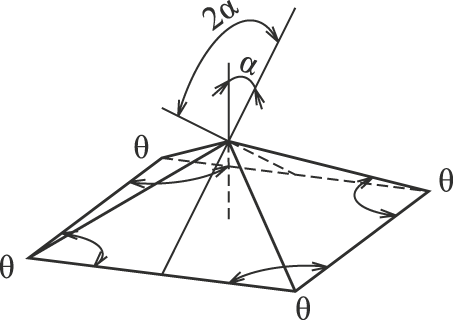
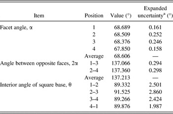
An example of evaluated Vickers pyramid geometry, illustrated in Fig. 4, is demonstrated in Table IV along with the estimated uncertainty. The expanded uncertainty for 95% confidence level is calculated by multiplying the standard uncertainty by the coverage factor corresponding to the effective degree of freedom, which is estimated with Welch–Satterthwaites equation.11
Geometrical parameters of Vickers indenter.
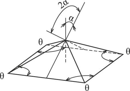
An example of the analysis of facet angles of a Vickers indenter.

a Coverage factor of 1.96.
IV. AREA FUNCTION CALIBRATION
The area function is the projected or surface area of indenter, which contacts with specimen, expressed as the function of the penetration depth. Since the indentation size is not measured directly in IIT, this indenter property is necessary to calculate hardness values or other material parameters.
Practically the area function is calibrated via indirect method such as indentation to some standard sample whose mechanical property is well known. These indirect methods, however, include theoretical assumptions, and if the assumptions are not appropriate, inconsistent results may be obtained such as the fake indentation size effect in indentation modulus.Reference Ishibashi, Ohki, Takagi, Yoshikawa, Katayama, Iwatsubo and Fujitsuka3 That’s why direct calibration of the area function with an AFM is preferable to obtain true material parameters.
To calculate the projected area function A P(h) from the AFM image, the unit areas of pixel of AFM image

are summed up from the tip of the pyramid to designated indentation depth h. This operation brings the projected area.

where Δx and Δy are the image resolution in x- and y-direction, respectively.
If the slope of the pixels is considered when summing up the unit area of pixels like

the surface area function can be obtained, where

is the slope of pixel i.
Figure 5 represents an example of the area function. The square root of projected area A P(h) is plotted against the contact depth h. If an indenter has ideal shape as specified in ISO standard, this representation should be a straight line starting from the origin of the chart. In reality, the indenter tip is not perfectly sharp and the slope in the vicinity of the origin is quite different from other part of the line. So, if the line is fit to the straight line expressed as

An example of the evaluated area function.

the truncation length Δh of the indenter can be obtained.
If an indenter has an ideal shape, its area functions are expressed as follows:


where C 0 and  are the constants depending on the facet angles of pyramids and

for Vickers and modified Berkovich indenters, or

for perfect Berkovich indenter, and

for Vickers and Berkovich indenters.
Then, the standard uncertainty of area functions can be estimated as follows:


where u(z) is the uncertainty of z-axis and equivalent to u meas,i (z) as previously derived.
Figure 6 represents an example of the standard uncertainty of projected area A P (h) and the relative standard uncertainty

Evaluated uncertainty of measurement of the area function.

As seen in the figure, the uncertainty u(A P) is nearly proportional to the contact depth h, whereas the relative uncertainty u rel (A P) increases exponentially, where h is small.
V. INDENTER GEOMETRY IN THE VICINITY OF THEIR TIP
Recently, the resolution of nanoindentation machine is revolutionary improved and indentation curve (force–depth) can be observed in the range of h<10 nm. For such a small range, the indenter geometry is no longer pyramidal; and in some specimens, no plastic deformations are observed because the tip is not sharp enough to cause plastic yielding. It suggests to us that it is suitable to evaluate the indentation modulus of thin layer by very shallow indentation.
It is known that the elastic response of contact between the indenter and the specimen depends on the geometry of indenter. For example, when the indenter has a sphere shape, the elastic behavior is described with Hertz’s contact theory,Reference Timoshenko and Goodier12 and when the indenter has a cone shape, the behavior is described with Sneddon’s theory.Reference Sneddon13 In reality, the geometry of the indenter tip is however neither sphere nor cone.
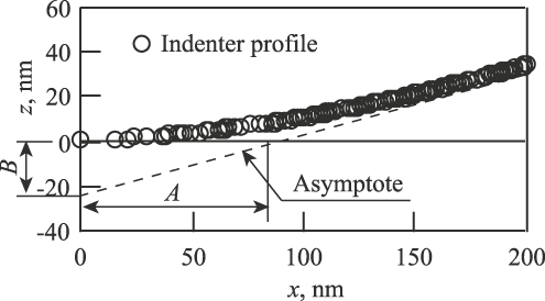
To describe the elastic behavior with real indenter geometry, Ishibashi et al.Reference Ishibashi, Ohki, Katayama and Takagi14 proposed the indenter model which has the hyperboloid shape and developed the contact theory between this indenter model and specimen. In this model, the indenter geometry is expressed as
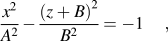
where A and B are the constants determined from AFM image. The graphical representation of Eq. (32) is shown in Fig. 7. The symbol B has the same meaning of Δh in Eq. (23) in a sense. Because the facet angles of pyramid are not constant (in general, it is larger in closer range to the indenter tip), Δh value varies depending on its range for analysis. On the other hand, B value is determined in very small range around the indenter tip where the deformation of samples occurs perfectly elastic.
Hyperboloid model of the indenter tip profile.
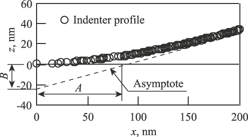
Ishibashi et al. also reported that the predicted elastic response with hyperboloid model agrees with experimental indentation curves very well.
VI. AFM OBSERVATION OF INDENTS
It is known that the material deformation around an indent is different according to its mechanical properties and can be categorized into sink-in mode or pile-up mode. In the history of the nanoindentation research, there are much knowledge in case of sink-in mode material such as glasses and minerals. On the other hand, metallic materials like steel have been used as hardness reference blocks for long time, and there are also much knowledge of manufacturing and handling those materials. For this reason, there are several attempts to use single crystalline or polycrystalline metal as the reference standards of IIT. Before such metallic materials are used as reference standards (CRMs), their deformation behaviors should be studied well. AFM observation of indents brings useful information about materials behavior and would help us to understand their indentation curves.
Observed image of a Vickers indent on a BK7 glass sample with an AFM is shown in Fig. 8. It is showing typical sink-in mode deformation.
AFM image of a Vickers indent on BK7 glass in the field of view of 15.1 × 15.1 μm2. (a) Three-dimensional (3D) view of the indent. (b) Cross-sectional profile.

On the other hand, observed image of a Vickers indent on a tool steel sample with an AFM is shown in Fig. 9. It is showing pile-up mode deformation. Comparing those two indents, the contact areas between samples and an indenter seem to be quite different and indentation hardness H IT or indentation modulus E IT values of those two materials could not be calculated with the same equation.
AFM image of a Vickers indent on the tool steel in the field of view of 34.9 × 34.9 μm2. (a) 3D view of the indent. (b) Cross-sectional profile.

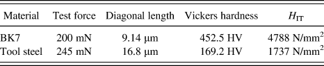
ISO 14577-115 suggests, however, that “H IT may be correlated to Vickers hardness” with the relation of

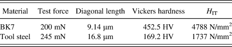
It means that if Vickers hardness of CRMs is determined through direct observation with an AFM, H IT values of them could be verified. Examples of calculated Vickers hardness and converted H IT of indents shown in Figs. 7 and 8 are listed in Table V. If the similarity of the indent on the same material is assumed, the result demonstrates the possibility to make up the verification table for some materials used as CRMs.
Examples of the conversion from Vickers hardness to H IT of CRMs.
VII. CONCLUSIONS
In this article, it is shown that the AFM is the useful tool to verify IIT indenters in micro- to nanorange. To verify the indenter geometry such as facet angles, angles between opposite faces and interior angles of the square base of pyramid, the fully mathematical method, which the author named as Regression Polyhedral Model, is used. The results obtained with this method is demonstrated with the uncertainty estimation. The uncertainty of measurement of the indenter geometry is the combination of the resolution and linearity of AFM, the uncertainty of the reference standard used to calibrate the AFM, the effect of the scanning tip, and the regression error. The results show that the uncertainty of facet angles and angles between opposite faces is small, whereas the uncertainty of interior angles of the square base of pyramid is not negligible.
The area function of an indenter is also demonstrated with its uncertainty. It was found that the uncertainty itself is nearly proportional to the contact depth but the relative uncertainty is exponentially increasing where the contact depth is small.
Expression of the indenter geometry in the vicinity of its tip is introduced in the form of hyperboloid.
To understand the difference of deformation mode of CRMs, indents made on different materials are observed with the AFM. By using conversion from Vickers hardness measured with the AFM to H IT, the possibility to verify the certified values of CRMs is suggested.
ACKNOWLEDGMENT
The author would like to thank Prof. T. Ishibashi of Niigata University for generous advices to complete this work and Mr. S. Katayama of Fischer Instruments, K. K. for the technical support.