1. Introduction

In curve fitting we are given a set of points in a plane spanned by an explanatory and an explained variable and then choose a curve that best expresses the systematic relation among them. For example, we might plot the yearly number of accidents with claimable damage against the total distance covered by the vehicle. What then needs to be determined is the functional dependence between frequency and distance. Since vehicles that do not cover any distance will not incur any damage, the intercept will be zero. The supposition may be that the dependence is linear, so that the choice concerns the slope of the line that relates distance to expected number of accidents. We might also postulate a more complicated relation between distance and expected number of accidents, for example, a quadratic dependence, perhaps with the idea that long-distance drivers have proportionally fewer accidents.

The general shape of a curve may be chosen at the outset, but sometimes the shape itself is under scrutiny. For example, we might compare the linear and the quadratic shapes sketched above. Statistical model evaluation allows us to compare such families of curves on a variety of performance measures. Model evaluation is important for scientists and philosophers of science alike. It allows scientists to submit their modeling assumptions to empirical testing and thereby address the uncertainty over their theoretical suppositions. Examples of such model evaluations abound, ranging from climate science and ecology to psychiatry and computational archaeology. Moreover, model evaluation gives philosophers of science a concrete and formally precise handle on a fundamental kind of uncertainty in science. Philosophers can motivate and develop norms for dealing with this uncertainty, which has direct relevance for the practice of science.

This article contributes to our understanding of the norms that drive statistical model evaluation. After an introduction into model evaluation tools in section 2, I present a problem for them in section 3. I then offer a diagnosis of the problem in section 4. In section 5 I show that the problem can be avoided if we involve prior probability assignments in the model evaluation. Throughout, I mostly avoid mathematical detail, to leave more space for conceptual considerations.

2. Statistical Model Evaluation

Statistical inference is carried out on the basis of a model, for example, by getting the data to choose among the hypotheses in the model or by redistributing the probability assignment over the hypotheses in the model. The curve fitting sketched in the introduction may not seem like a statistical inference. Given a family of curves, we simply choose by minimizing the errors, that is, the sum of the discrepancies between curve and point. In the so-called least-squares approach, for example, the error is calculated as the sum of the squares of the vertical distance between point and curve. No model seems to be involved in this.

Underneath such a minimization procedure, however, we do find a statistical inference. One central modeling assumption is that the explained, or dependent, variable Y follows some unimodal probability distribution, for example, a normal distribution N(μ,σ). A further assumption is that the mean of this distribution depends on the explanatory, or independent, variable X. For example,

(1)$\begin{array}{}{P}_{\theta }\left(Y|X\right)=N\left(\mu \left(X\right),1\right),\end{array}$

with $\mu \left(X\right)={\theta }_{1}X+{\theta }_2{X}^2$, for example, and Y standardized to make $\sigma =1$. Note that the model dictates a distribution over Y for all values of X but that it does not determine a probability distribution over the values of X itself. The distance X is an explanatory variable, and we presume that it is randomly sampled from a uniform distribution.

The data consist of m points in the plane 〈X, Y〉, collected in a scatter plot:

(2)$\begin{array}{}{S}_{\mathrm{XY}}=\left\{〈x_1,y_1〉,〈x_2,y_2〉,\dots ,〈x_m,y_m〉\right\}.\end{array}$

For any curve and associated hypothesis we can calculate the probability of a scatter plot, that is, the likelihood of the hypothesis for the data, by multiplying the probability of all the points,

(3)$\begin{array}{}{P}_{\theta }\left(S_{\mathrm{XY}}\right)=\prod _{i=1}^m{P}_{\theta }\left(y_i|x_i\right).\end{array}$

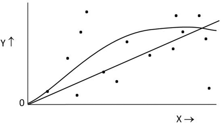
To fit the curve we look for the value of θ, denoted $\hat{\theta }$, that makes the probability of the scatter plot maximal. Generally speaking, maximizing the likelihood of the curve will correspond to minimizing the vertical distance of points to the curve under some notion of distance. Figure 1 offers an impression of what these curves may look like.

Figure 1.

Polynomial curves fitted to the scatter plot.

Against this background of curve fitting as statistical inference, it will be clear that evaluating the general shape of the curves, for example, comparing linear and quadratic ones, is part of statistical model evaluation. Note that I use the term “model evaluation,” not the more often used “model selection.” Selecting a model would seem a decision and so involves decision-theoretic as well as inferential aspects. But in what follows I only consider norms for the comparison of models from an evaluative, epistemic standpoint.

A very common idea about model evaluation is that, next to the fit with data, it involves the complexity of the model. If a neat fit with the data is achieved by adding many bells and whistles, we are rightly reluctant to put our trust in it. We then say that the model is fitting to noise, or overfitting. In the example, the best fitting curve from the quadratic model will have a higher likelihood than the best curve from the linear model. But this is not to say that the quadratic curve is better. The question is whether the gain in fit weighs up against the cost of a more complicated model.

The extant model evaluation tools, most notably the various information criteria (Claeskens and Hjort Reference Claeskens and Hjort2008), provide specific formats for this trade-off between simplicity and fit. The two most prominent tools, the Akaike and Bayesian information criteria (AIC and BIC, respectively), express the simplicity by means of the number of free parameters in the model (e.g., Akaike Reference Akaike, Petrov and Csaki1973; Schwarz Reference Schwarz1978; Raftery Reference Raftery1995; Burnham and Anderson Reference Burnham and Anderson2002). The linear model of the example has one free parameter, and the quadratic model has two. The ICs then differ in how they factor the number of parameters into the trade-off:

(4)$\begin{array}{}\mathrm{AIC}\left({ℳ}_{\theta }\right)=2\log \left(P_{\hat{\theta }}\left(S\right)\right)-2\dim \left({ℳ}_{\theta }\right),\end{array}$

(5)$\begin{array}{}\mathrm{BIC}\left({ℳ}_{\theta }\right)=2\log \left(P_{\hat{\theta }}\left(S\right)\right)-\log \left(m\right)\dim \left({ℳ}_{\theta }\right),\end{array}$

in which ${ℳ}_{\theta }$ is the model parameterized by the vector θ, the number of free parameters is given by dim(${ℳ}_{\theta }$), and $\hat{\theta }$ is the hypothesis in the model with maximum likelihood for the data S, so that $P_{\hat{\theta }}\left(S\right)$ is the likelihood of the maximum likelihood estimator for the data S. In the BIC the penalty for complexity is scaled according to the sample size of the data m.

The involvement of the complexity of models in their evaluation may seem intuitive on pragmatic and metaphysical grounds. A simpler model is easier to use, and we might think that the world itself is a simple place, perhaps because the demiurge is an efficient or lazy being. However, the actual reason for the appearance of the complexity penalty in the ICs is epistemic. For example, the number of parameters appears in the AIC as a result of approximating the expected Kullback-Leibler divergence to the true hypothesis. And for the BIC the penalty for complexity drops out of an approximation of the past predictive performance of the model, as measured by the marginal likelihood.

The number of model parameters surfaces repeatedly as a criterion for model evaluation, under a variety of epistemic good-making features of models. Very roughly, the underlying reason is that the predictions and general empirical claims of more complex models will be less robust and reliable. In a more complex model the same number of data points will be used to determine a larger number of parameter values, and therefore, speaking metaphorically, the available information will have to be spread more thinly. For the AIC this shows up in the relative uniformity of the likelihood function over the model, and in the BIC it appears as the relative uniformity of the posterior probability distribution within the model. The general idea is that we can always introduce an additional parameter that improves the best fit in the model but that we might then lack the data to properly back up a stable value for this additional parameter.

However, this intuition does not cover everything that is salient about complexity in model evaluation. There is another epistemic good-making feature, strongly related to complexity and the number of parameters, that needs to be taken into account when we compare models. This further feature concerns something like model size. It can be expressed by means of the prior probability distribution within the models, as the following model evaluation problem will reveal.

3. Cheap and Almost Perfect Fit

Consider again the example of the scatter plot and the polynomial model. But instead of using the polynomial curves, as detailed above, imagine fitting the data with a model based on trigonometric functions, or sine curves (e.g., Harman and Kulkarni Reference Harman and Kulkarni2007, chap. 3). We use the normal distributions of equation (1), but instead of choosing μ(X) to be polynomial we choose

(6)$\begin{array}{}\mu \left(X\right)={\alpha }_1-{\alpha }_1\cos \left({\alpha }_{2}X\right).\end{array}$

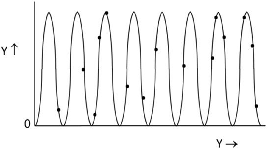
Figure 2 gives an impression of the fit that may be achieved by the so-called sine model. Importantly, all the points in the scatter plot are given close to maximal probability, because they all end up sitting arbitrarily close to the curve, and hence to the mean for the distribution.

Figure 2.

Sine curve that perfectly fits the scatter plot.

The key observation is that we have achieved this remarkable fit at the expense of only two parameters, α₁ and α₂. It is known that we can obtain a perfect fit to m data points with a polynomial curve that has m free parameters. But fitting any number m of points with two parameters seems inexplicably efficient. Clearly, if we were to apply model evaluation criteria like AIC or BIC, or indeed any other method in which complexity is expressed by the number of parameters, the sine model wins out on the quadratic model and most likely also on the linear model. What is going on?

Before providing a diagnosis, let me emphasize that the claim that a near-perfect fit is always possible is mathematically nontrivial. In the remainder of this section, I provide more detail to substantiate it. Notably, the fit does not hinge on the assumption of any particular distribution, be it normal, Poisson, or otherwise, or on any particular format of the data, be it real numbers, integers, or otherwise. Moreover, given that the scatter plot will manifest on a finite domain $0<X<L$ we need not even suppose that the parameters are real valued: it is enough to consider sine curves with a period $L/t$ for $t\in \mathbb{N}$, as one does in a Fourier series. Despite all this, it turns out that there are always infinitely many almost perfect fits to a set of points. This abundance of solutions will turn out to be of crucial importance for the resolution of the problem.

Say that we have been given a scatter plot S_XY whose farthest points are at $x_i=L$ and $y_j=H$. For convenience we set ${\alpha }_1=H/2$, but any α₁ larger than that will work too. Take any specific point 〈x, y〉 from the scatter plot, consider the curves with ${\alpha }_2=L/t$ for increasing t, and ask: for what values of t does the sine curve intersect with the line $X=x$ in very close proximity to the value y? Observe that $x\in \left[\mathrm{kL}/t,\left(k+1\right)L/t\right]$ for some t and that the curve covers the whole of the range [0, H] over this interval of X twice. If we allow for a discrepancy of ε between the curve and the value y and assume that x falls within the first half of the interval, we must require that

(7)$\begin{array}{}\frac{L}{\pi t}{\cos }^{\mathrm{-1}}(1-\frac{2\left(y-\epsilon \right)}{H})<x-\frac{\mathrm{kL}}{t}<\frac{L}{\pi t}{\cos }^{\mathrm{-1}}\left(1-\frac{2\left(y+\epsilon \right)}{H}\right).\end{array}$

If x falls in the second half of the interval [$\mathrm{kL}/t$, $\left(k+1\right)L/t$], we require an analogous constraint. Because the slope of the cosine is bounded between −1 and 1, we may replace the above inequalities with

(8)$\begin{array}{}{X}_B-\frac{2\epsilon L}{\pi \mathrm{tH}}<x-\frac{\mathrm{kL}}{t}<X_B+\frac{2\epsilon L}{\pi \mathrm{tH}},\end{array}$

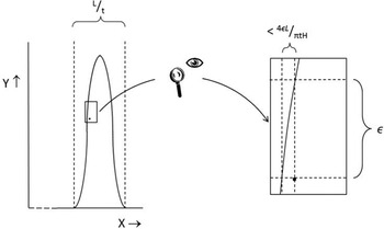
in which $X_B=(L/\pi t){\cos }^{\mathrm{-1}}\left(1-(2y/H)\right)$, and similarly for x sitting in the second half of the interval. Consequently, for every t there is a specific region of length $4\epsilon L/\pi \mathrm{tH}$ within the interval of length $L/t$ such that, if it includes x, the resulting distance of the curve to y lies within an ε bound. Figure 3 gives an impression of the above construction.

Figure 3.

Sine curve that passes a point at distance ε.

The remaining question is whether and for what values of t the value x lies within this specific region. To establish that, we first recall that the x_i’s from the scatter plot S_XY were randomly sampled from a uniform distribution over [0, L]. This means that the individual x from the sample is almost surely, that is, with probability 1, a random number. Consequently, there will be no pattern in how x shows up inside the intervals [$\mathrm{kL}/t$, $\left(k+1\right)L/t$] for increasing t. The locations of x are evenly distributed over all parts of these intervals. Hence, for any $\epsilon >0$ there will be infinitely many t for which x will fall within the portion of length $4\epsilon L/\pi \mathrm{tH}$ inside the interval of length $L/t$. The relative size of the region in which the curve is sufficiently close to the value y is constant for increasing t at $4\epsilon /\pi H$. And so there will be infinitely many sine curves that have an arbitrarily small error in fitting the point 〈x, y〉.

This suffices as an argument for there being an infinity of curves that fit any finite number of points almost perfectly. For a single point, the fraction of sine curves will tend to $4\epsilon /\pi H$. So for a set of m points that are randomly distributed over X, the fraction will tend to ${\left(4\epsilon /\pi H\right)}^m$. When making ε small and thus maximizing the likelihoods, the fraction of curves with good enough fit will be very small. But there will still be infinitely many fitting ones.

4. Diagnosis of the Problem

The foregoing construction presents a problem for standard model evaluation tools. The BIC simply rules in favor of the sine model. The AIC is not defined for unidentified models, so the fact that there are infinitely many equally well-fitting sine curves incapacitates it. While silence is better than positive evaluation, a negative evaluation of the intuitively incorrect sine model would seem best. Closer inspection reveals that the sine model is not robust, that its dimensions are deceptive, and that it is not well behaved under increases in data size. Fortunately these considerations set us up for a solution to the problem along Bayesian lines in the next section.

First consider the robustness of the sine model. Imagine that we alter the scatter plot by slightly nudging a single data point. What will be the result if the curve is a polynomial of a given degree? Clearly, any curve that was fitted to the data will change a little as well. But the rough shape of the curve will not change a lot: a small change in data is matched by a similarly small change to the best fitting curve. By contrast, if the curve is a trigonometric function, then nudging a single data point slightly will radically alter it. Nudging leads to a completely new set of best fits. We might say that the sine model is skittish, or too versatile, or lacking in robustness: it is oversensitive to the smallest of changes in the scatter plot.

The AIC and BIC do not accommodate this feature of models. Minimum description length (MDL) based model evaluation tools and extensions of the AIC and BIC fare slightly better. The so-called Fisher information (FI) approximation, for example, includes a geometric complexity term, based on the FI. One might say that the FI expresses how densely packed the model is with likelihood functions (Myung et al. Reference Myung2000; Grunwald Reference Grunwald2007; Ly et al. Reference Ly, Verhagen, Grasman and Wagenmakers2017). Inclusion of the FI will penalize skittish models, because these models cover a larger set of data patterns, and in this sense they are indeed packed more densely. Furthermore, developing the AIC and the BIC (cf. Bozdogan [Reference Bozdogan1987] and further references therein), we also encounter the FI. So there are natural extensions of the AIC and the BIC that accommodate something of the skittishness.

However, in all of these refined methods, the contribution of the FI term is not of the required order of magnitude to resolve the problem of the sine curves. Apart from the original AIC, the FI term is trumped by the term that captures complexity as the number of free parameters, which grows with log(m). And the FI term cannot compete with the fit term, which grows with m in all model evaluation tools. For larger data sets the influence of the FI term on the model score therefore dwindles, so that the sines seem preferable after all.

A second consideration concerns the deceptively low dimensions of the sine model: it seems to harbor an inherent complexity that is not expressed in the number of parameters. The sine model illustrates that model dimension is a fleeting notion. As a quick illustration, note that statistical parameters are often real numbers. But real numbers are such that we can package any amount of information into them. For example, a sufficiently complicated function will allow us to compact two real numbers in a single one, by constructing the numerical expansion of a number from two such expansions (e.g., 0.135 … and 0.246 … yield 0.123456 …), and so on. While this sort of function is of course hopelessly contrived, it illustrates that counting statistical parameters does not give us a fair indication of model dimensions.

This has been observed about model evaluation criteria more often, for example, in Bozdogan (Reference Bozdogan1987), who proposes to adapt the AIC by involving the sample size, thereby bringing it closer to the BIC. His motivation for adapting the penalty term is, by and large, that the notion of complexity is not adequately captured by the dimension term in the original AIC. Similar sentiments are expressed by Balasubramanian (Reference Balasubramanian and Grunwald2005), who develops an MDL approach, and in Romeijn and van de Schoot (Reference Romeijn, van de Schoot, Hoijtink, Klugkist and Boelen2008) and Romeijn, van de Schoot, and Hoijtink (Reference Romeijn, van de Schoot, Hoijtink, Dieks, Gonzales, Hartmann, Stadler, Uebel and Weber2012), in which the BIC is investigated and extended. The latter two point to a more general notion of model size as a component of complexity. However, while these proposals are in the right direction, the adapted versions of AIC, BIC, and MDL still give the number of parameters a central role.

A more promising method for dealing with the problem of the sine curves is perhaps offered by the so-called deviance information criterion (DIC; Spiegelhalter et al. Reference Spiegelhalter, Best, Carlin and van der Linde2002). The DIC was originally designed for comparing hierarchical Bayesian models, in which the number of free parameters is not clearly defined. Central to the DIC is the so-called deviance, which can be roughly understood as the reduction in surprise due to estimation, and hence as a degree of overfitting. The penalty for complexity in the DIC is determined by the effective number of parameters, which is based on the notion of deviance. It would seem that the DIC responds correctly to the sine model, but the details of this must be left to future research. The current purpose is not to advise practitioners on the IC of choice but to offer a conceptual analysis of the inadequacy of the sine model.

A final consideration brings us closest to this goal. Note that both polynomial and trigonometric curves can be used as a basis for the space of functions on a finite domain, in the algebraic sense that they parameterize that space: we can write down functions by their Taylor or Fourier series. We can collect all the curves that fit some scatter plot almost perfectly into a set within the space of functions. But for the Taylor and Fourier series this set will look very different. In the Taylor parameterization, the set is a well-behaved region sitting somewhere in the linear combination of at least m axes. But the set of well-fitting curves will look much wilder and disjointed in the Fourier parameterization, disjointed and intersecting with distinct axes rather than being lumped together.

The implications of this are best brought out through a variant of the robustness discussed above, namely, by considering what happens if we start adding points in the scatter plot. The original polynomial curve will not change too radically: the region of well-fitting curves will shift only slightly. By contrast, the set of best fitting sine curves alters significantly with the addition of a point, not so much by being relocated but rather by being constrained severely. There are infinitely many sine curves that fit the scatter plot, but almost all of those curves will miss the additional point by a stretch and so be eliminated from the set of well-fitting curves. The solution of the problem hinges on exactly this elimination of hypotheses.

5. Priors to the Rescue

This section develops a particular response to the problem of the sine curves. It relies on so-called Bayesian model selection, or Bayesian model evaluation (BME). Following BME the sine model loses against polynomial models because of the specific failure of robustness introduced above.

The message of this section is not that we should embrace BME as the new standard in model selection. I will not make a systematic comparison with other model evaluation criteria and their relation to the salient notion of robustness. Looking at the solution that BME provides and the central role for the so-called marginal likelihood in BME, we might expect that other approaches in which the marginal likelihood is central (e.g., the DIC and MDL-based criteria but arguably also cross-validation) will provide a solution as well. Because we can only compute something like a marginal likelihood if we adopt some version of a prior within the model, the central point of this section is rather that solutions will have to rely on priors of some kind.

The central idea of BME is to compare models by their posterior probability assignment:

(9)$\begin{array}{}\frac{P\left({ℳ}_1|S_{\mathrm{XY}}\right)}{P\left({ℳ}_2|S_{\mathrm{XY}}\right)}=\frac{P\left({ℳ}_1\right)}{P\left({ℳ}_2\right)}\times \frac{P\left(S_{\mathrm{XY}}|{ℳ}_1\right)}{P\left(S_{\mathrm{XY}}|{ℳ}_2\right)}.\end{array}$

Assuming an equal prior for the models ${ℳ}_i$, the posteriors are completely determined by the ratio of the so-called marginal likelihoods,

(10)$\begin{array}{}P\left(S_{\mathrm{XY}}|{ℳ}_i\right)={\int }_{\Theta }P\left(H_{\theta }|{ℳ}_i\right)P\left(S_{\mathrm{XY}}|H_{\theta }\cap {ℳ}_1\right)d\theta ,\end{array}$

in which Θ is the parameter space. The likelihoods $P\left(S_{\mathrm{XY}}|H_{\theta }\cap M_1\right)$ are a different notation for the P _θ(S_XY) of the foregoing. Notice that the prior within the model, $P\left(H_{\theta }|{ℳ}_i\right)$, plays a key role in the computation of the marginal likelihood. Many approaches to model evaluation rely on the marginal likelihood of the model, including the BIC, the DIC, and MDL-based approaches. All these approaches must use some notion of a prior.

Now recall how sine curves manage to fit any scatter plots almost perfectly, in particular that there are infinitely many such curves. With the addition of a new point, this set of best fitting curves will lose a large number of members, and this will severely affect the marginal likelihood of the sine model. Following equation (3), we see that the likelihood of sine curves that retain their fit must be multiplied by a maximal probability for every new data point. But this only holds for a small fraction $4\epsilon /\pi H$ of the sine curves. The fraction $1-4\epsilon /\pi H$ of sine curves will be multiplied by a factor that falls very far short of the maximum probability.

By comparison, the likelihoods of well-fitting polynomial curves will pick up a factor that is somewhat lower than the maximal probability for each point, although not falling very far short of the maximum. Importantly, this high but not maximum factor will apply to a set of curves that is more or less stable and that will accumulate more and more probability with the addition of data points. Consequently, the overall factor picked up by the marginal likelihood of the polynomial models will tend to this high but not maximum factor.

To put this in a more mathematical format, say that the average factor picked up by the likelihood of a sine curve outside of the set of best fitting curves is U, that the same factor applies to badly fitting polynomial curves, that the factor for a reasonably well-fitting polynomial is V (and for a best fitting sine curve W), so that $U<V<W$. For the sine curves we obtain

(11)$\begin{array}{}P\left(〈x_{m+1},y_{m+1}〉|{ℳ}_{\mathrm{sine}}\cap S_{XY}\right)\approx \left(1-\frac{4\epsilon }{\pi H}\right)U+\frac{4\epsilon }{\pi H}W,\end{array}$

which is arbitrarily close to U. For the model M _poly with polynomial curves of a specific order, we will have

(12)$\begin{array}{}P\left(〈x_{m+1},y_{m+1}〉|M_{\mathrm{poly}}\cap S_{\mathrm{XY}}\right)\approx \left(1-R_m\right)U+R_{m}V.\end{array}$

The factor R_m stands for the probability of the region of hypotheses for which the fit with the m points is reasonably good. It is hard to say how this factor develops in general, but with the accumulation of data points, the set of well-fitting curves will generally stabilize, and hence R_m will tend toward 1 for increasing m. The result is that the sine model performs less well than the polynomial model on the BME criterion. On BME, therefore, the inherent complexity of the sine curves is adequately factored in.

It will be insightful to return to the observations that the set of well-fitting sine curves is skittish. Well-fitting polynomial curves of a given degree are located in a particular region within the model, in which posterior probability can accumulate when data size increases: they will respond to new data points in roughly the same way. By contrast, with every new data point a tiny fraction of the well-fitting sine curves is multiplied by a high likelihood, while the rest picks up a very low factor. It reveals the skittishness of sine curves that such a large portion of curves is suddenly far off in their prediction.

We can also convert this reasoning to arrive at the consideration on model size. Judged from a prior probability distribution within the sine model, the set of well-fitting curves is very small indeed: after m points it has decreased to ${\left(4\epsilon /\pi H\right)}^m$. But considering a prior within the polynomial model, the set of well-fitting curves retains a reasonable size. What this signals is that the sine model, although it has only two free parameters, has many more different statistical hypotheses packed into it. It is versatile at the cost of a particular kind of robustness. The use of a prior within the model enables us to bring this kind of robustness out.

6. Conclusion

We cannot turn the foregoing into an argument for BME: other model evaluation criteria may also have a response to the problem at stake. But there are several general lessons to take away. One is that we must never mistake the number of parameters in a model for its actual complexity. A related lesson is that we must not forget the deeper motivations for the model evaluation tools, that is, the good-making features that the tools are based on. Concentrating on those features will guide us to a better understanding of our evaluations.

Another general lesson ties in with earlier work on the role of size in model evaluation (Romeijn et al. Reference Romeijn, van de Schoot, Hoijtink, Dieks, Gonzales, Hartmann, Stadler, Uebel and Weber2012) and indeed with scientific methodology as a whole. In the solution of the problem with the sine model, we can recognize a Popperian theme. Models that allow for fewer possible data patterns are preferable to those that allow for a very wide range of data patterns. To express a notion of model size in our evaluations, we have to adopt some measure over the space of distributions over data. So we must involve something akin to a prior.

There is, however, a problem with the idea that we can objectively determine how densely distributions are packed together in a model. To say that a set of distributions shows a wide variety in the data patterns that it can adapt to, we need to presuppose a notion of similarity among data patterns or, more generally speaking, a metric over sample space. In this article that metric was adopted implicitly, as part of the way in which we depict and conceptualize the data. This dependence on the metric of the sample space points to a potential subjectivity in adjudicating between statistical models, or at least a reliance on a natural conceptualization of the sample space. This idea deserves to be studied in its own right.