





Impact statement
This study advances the understanding of floating solar photovoltaic (FSPV) systems by addressing their performance and reliability under high-humidity conditions typical of tropical environments. Beyond energy generation, the work highlights the role of FSPV in addressing land constraints, supporting the water–energy nexus and enabling sustainable infrastructure development in ecologically sensitive regions. By integrating environmental degradation into performance assessment, the study provides insights relevant for long-term system design, policy formulation and large-scale deployment of floating solar technologies in emerging energy markets.
Introduction
Energy is an indispensable resource crucial for sustaining modern society and driving global development, making a reliable supply a pressing global challenge (Mahadevan and Asafu-Adjaye, Reference Mahadevan and Asafu-Adjaye2007; Chen and Chen, Reference Chen and Chen2011). In 2024, global electricity consumption reached 29,000 TWh (International Energy Agency, 2024), with nonrenewable sources primarily coal (36.7%) and other conventional fuels (26.3%) dominating production (IEA, 2024; Ahmed et al., Reference Ahmed, Ge, Peng, Yan, Tee and You2022). Conventional energy sources, while economical, pose a major threat due to significant CO2 emissions, which drive global warming (Farghali et al., Reference Farghali, Osman, Mohamed, Chen, Chen, Ihara, Yap and Rooney2023; Rad et al., Reference Rad, Kasaeian, Niu, Zhang and Mahian2023). The resulting adverse effects, including natural calamities, soil degradation and ecosystem imbalance, necessitate an urgent global shift toward clean, inexhaustible and sustainable energy (Awaad et al., Reference Awaad, Mansour, Akrami, Fath, Javadi and Negm2020; Kumar et al., Reference Kumar, Kumar and Pal2021; Naeem and Arfaoui, Reference Naeem and Arfaoui2023). Renewable sources (solar, wind and hydro) limit greenhouse gas emissions and are essential for mitigating the degradation of life on earth (Yoro and Daramola, Reference Yoro, Daramola, Rahimpour, Farsi and Makarem2020; Olczak et al., Reference Olczak, Żelazna, Matuszewska and Olek2021). Currently, solar power contributes only 5.3% of total energy generation (Ahmed et al., Reference Ahmed, Ge, Peng, Yan, Tee and You2022; Yu et al., Reference Yu, Du, Chen, Su, Zhang, Yang, Wang and Zhang2022), highlighting the vast potential for expansion.
The abundance of sunlight makes it obvious that harnessing solar power is a vital step toward renewable energy generation. The factors affecting the output of photovoltaic (PV) cells are solar irradiance, sunshine duration, angle of incidence of sunlight, PV module temperature, dust and dirt deposition on the panel, shading effect and inverter efficiency (Sharma et al., Reference Sharma, Jalil, Ansari and Bansal2023; Yadav et al., Reference Yadav, Pal, Khan, Parihar, Khan, Solanki, Pansari, Sharma and Yadav2025). Byrack et al. (Reference Bayrak, Oztop and Selimefendigil2019) discussed the effect of temperature on the performance of PV modules. The authors found that the heat due to solar radiation is not spread evenly across the module. Cooling the PV module by passive methods like adding aluminum fins on the backside of the solar cell increases the power output by 5.5%. Adinoyi and Said (Reference Adinoyi and Said2013) studied the effect of dust deposition on solar panels. They found that the power output of the PV module is decreased by 50% when left uncleaned for over 6 months in the Gulf region, and the implementation of a solar tracker has helped to decrease the dust deposition. Similarly, Kazem et al. (Reference Kazem, Al-Waeli, Chaichan, Sopian, Gholami and Alnaser2023) experimented on 100 W PV modules in Oman and found that the output decreased by 40% due to dust deposition. Shading of PV modules causes a significant loss of power output even at a very small area of shading (Trzmiel et al., Reference Trzmiel, Głuchy and Kurz2020).
Government policies and technological advancements have been pivotal in promoting solar PV technology. Improvements in semiconductor technology have driven an exponential decrease in PV module prices and a simultaneous increase in efficiency (Babich et al., Reference Babich, Lobel and Yücel2020). Given India’s rapidly increasing energy demand and its favorable tropical location with abundant sunlight (Rauf et al., Reference Rauf, Nureen, Irfan and Ali2023; Bhattacharya et al., Reference Bhattacharya, Sadhu and Goswami2024), solar energy is a strategic resource. However, conventional land-based PV (LBPV) deployment is constrained by the scarcity and high cost of land (Goswami et al., Reference Goswami, Sadhu, Goswami and Sadhu2019). Floating solar photovoltaic (FSPV) systems address this challenge by utilizing the surface area of water bodies like reservoirs, mitigating the land acquisition problem associated with LBPV (Goswami et al., Reference Goswami, Sadhu, Goswami and Sadhu2019).
FSPV relies on various floater mechanisms, predominantly pontoon-based floaters made of high-density polyethylene (HDPE). HDPE is lightweight, economical and corrosion-resistant, but its structural strength is limited, making it susceptible to UV damage, biofouling and mechanical stress (Dai et al., Reference Dai, Zhang, Lim, Ang, Qian, Wong, Tan and Wang2020; Khan and Sahai, Reference Khan and Sahai2024). Alternative options include metal-based floaters, which offer superior strength but face corrosion challenges (especially in saline water) (Oliveira-Pinto and Stokkermans, Reference Oliveira-Pinto and Stokkermans2020), and durable but heavy concrete-based floaters (Huang et al., Reference Huang, Tang, Chen, Chen and Jiang2023). Advanced designs, such as Swimsol (styrofoam-based for high waves) and Heliofloats (air-cushion based) (Oliveira-Pinto and Stokkermans, Reference Oliveira-Pinto and Stokkermans2020; Djalab et al., Reference Djalab, Djalab, El Hammoumi, Tina, Motahhir and Laouid2024), are emerging to expand FSPV applicability to challenging marine environments.
Sukarso and Kim (Reference Sukarso and Kim2020) found that FSPVs stay cool as they are floated on water bodies, which gives an added advantage of increased power output than LBPV modules. Setting up FSPV on large water bodies ensures that there will be no shading on PV modules (Sasmanto et al., Reference Sasmanto, Dewi and Rusdianasari2020). Rehman et al. (Reference Rehman, Irshad, Mohandes, Al-Shaikhi and Zayed2024) performed a comparative analysis of land-based PV systems and FSPV systems in Saudi Arabia. The authors found that the FSPV system was cooler by 7.5–21.3% than the ground-based system, which enabled the FSPV system to operate with 12.2% higher efficiency. A study by Singh et al. (Reference Singh, Goswami and Sadhu2024) showed that even after considering water-based degradation, FSPV system operates with 4–5% higher efficiency than a similar land-based system.
FSPV also helps to diminish the evaporation of water from water bodies and helps in water conservation, thus satisfying the aims of SDG 7. SDG 7 is one of the 17 goals established by the United Nations (UN) as part of the 2030 Agenda for Sustainable Development. SDG 7 seeks to ensure access to affordable, reliable, sustainable and clean energy for all. It focuses on expanding the proportion of renewable energy and raising energy efficiency. Realizing SDG 7 is central to clean energy generation, poverty reduction and mitigating climate change (Vidović et al., Reference Vidović, Krajačić, Matak, Stunjek and Mimica2023; Singh et al., Reference Singh, Goswami and Sadhu2024). FSPV systems have all these advantages, which make it a viable choice for renewable energy generation as it complies with the aims of SDG 7.
Despite all the advantages, FSPV systems are uniquely susceptible to water-borne degradation mechanisms, including physical, chemical and biological stressors that differ from those affecting ground-mounted panels (Liu et al., Reference Liu, Pan, Huang, Sun, Gu, Zhuang and Wang2024). A primary concern is humidity-induced degradation, as continuous high ambient moisture exposure allows water vapor to penetrate the encapsulant. This moisture ingress facilitates internal module damage, such as delamination, corrosion of metal contacts and breakdown of electrical insulation, leading to hot spots and overall efficiency loss (Naushad et al., Reference Naushad, Rimon and Khan2025). Furthermore, the perpetual damp environment accelerates corrosion in metallic components (frames and mounting systems), sparking electrochemical oxidation (Kumar et al., Reference Kumar, Pachauri, Kuchhal and Nkenyereye2025; Wei et al., Reference Wei, Khojasteh, Windt and Huang2025). Over time, water vapor migration through protective coatings can cause dangerous localized corrosion, particularly crevice corrosion, in low-evaporation areas like under bolts and junction boxes, which can lead to extensive, undetected structural failure (Attar et al., Reference Attar, Alahmer, Borowski and Alsaqoor2025; Saw et al., Reference Saw, Heng, Leow, Nairi and Pravettoni2025). Luo et al. (Reference Luo, Isukapalli, Vinayagam, Ting, Pravettoni, Reindl and Kumar2021) reported performance loss rates of ~0.5–0.7% annually for floating PV systems. However, these values were found to be comparable to nearby rooftop PV systems, suggesting that the observed degradation was not uniquely attributable to the floating environment. Similarly, Goswami and Sadhu (Reference Goswami and Sadhu2021) performed an extensive study of the FSPV system and found that water-based corrosion reduced the performance of FSPV systems. This also affected the total life of the utility-based FSPV power plants. Sahu and Sudhakar (Reference Sahu and Sudhakar2019) found that UV and humidity corrode the floats affecting the performance of FSPV systems. Kowsar et al. (Reference Kowsar, Hassan, Rana, Haque, Faruque, Ahsan and Alam2023) assumed an annual degradation rate of 0.72% in their PVsyst-based simulation of a proposed FSPV system in Bangladesh. This value represents a modeling input rather than an experimentally measured field degradation rate. Water quality majorly affects the performance of FSPV systems. Singh and Sadhu (Reference Singh and Sadhu2024) studied FSPV systems in India and found that the FSPV system had an annual loss of energy of 4.07% due to water salinity. Dzamesi et al. (Reference Dzamesi, Ahiataku-Togobo, Yakubu, Acheampong, Kwarteng, Samikannu and Azeave2024) studied the FSPV system at Bui Generating Station, Ghana, and found that the humidity at the FSPV site was 73% and 62% at the LBPV site.
Humidity-induced degradation extends to corrosion under insulation, where water penetrates insulated or enclosed system areas, causing hidden corrosion and creating short-circuit or fire hazards, especially in electrical connectors and junction boxes. Accelerated corrosion tests, such as those proposed by Liu et al. (Reference Liu, Kong, Kao and Wu2021), are essential for accurately predicting component reliability. Studies comparing degradation have shown significant differences; for example, Mannino et al. (Reference Mannino, Tina, Cacciato, Merlo, Cucuzza, Bizzarri and Canino2023) found an offshore FSPV degradation rate of 0.95% versus 3% for an onshore system, underscoring the necessity of anticorrosive coatings and superior sealing in FSPV design.
Previous research has largely considered the FSPV performance, attributing it to water corrosion and the effects of the surrounding environment. This analysis offers a different approach, where humidity is considered the main degradation cause. In contrast to previous work, the present work typically links degradation to wide water-induced phenomena and long-term corrosion signatures. Such a targeted effort promotes the predictive knowledge of the performance degradation and reliability problems of the FSPV systems. A comparative analysis between FSPV and conventional land-based PV systems is also conducted to highlight differences in efficiency, energy yield and system behavior under identical environmental conditions. Furthermore, the study integrates both economic and environmental assessments to evaluate the effect of humidity on FSPV systems and the overall feasibility of FSPV deployment considering humidity-based performance degradation. This holistic approach not only fills a critical knowledge gap but also provides valuable insights for policymakers, engineers, researchers and stakeholders aiming to understand and promote the large-scale adoption of FSPV systems in real outdoor conditions.
The remaining article is structured as follows: Section “Mathematical modeling of solar module” discusses the mathematical analysis to determine the performance of the PV cells. Section “Location and meteorology” describes the site selection and the design of the FSPV system. Section “Result and discussions” covers the performance analysis of the FSPV system, including the environmental and economic analysis. The conclusion is provided in Section “Discussion.”
Mathematical modeling of a solar module
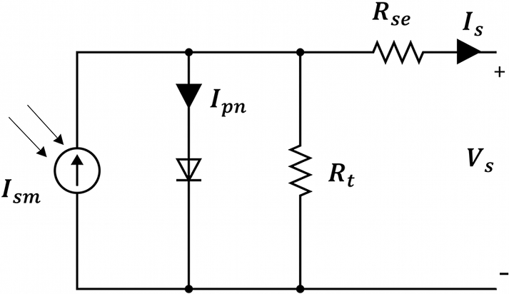
A solar cell is a PN junction where electricity is produced when there is incident light on it. The basic modeling of this solar cell is represented in Figure 1 by a current source with a resistance in series (R se) along with a parallel shunt resistance (R t) (Ebhota and Tabakov, Reference Ebhota and Tabakov2023). Shunt or parallel resistance basically denotes the leakage currents and other resistances. Series resistance is primarily the total resistance between the P layer and N layer of the cell; it also considers the resistances between each layer and the metal frames (Ma et al., Reference Ma, Gu, Shen and Li2019).
PV cell structure.

The output current of the solar cell (I s), given in Eq.1, is calculated by applying Kirchhoff’s current law (KCL) (Nguyen and Nguyen, Reference Nguyen and Nguyen2015; Ma et al., Reference Ma, Gu, Shen and Li2019).

where I
sm is the photocurrent, I
pn is the diode current and the current through the shunt resistance is I
t.
$ {I}_{pn} $
 is the current flowing through the diode. By further substitution, I
s can be written as:

Applying the Shockley equation for the diode:

where I
rs represents the saturation current of the diode in the reverse direction. Vth is the thermal voltage, n is the ideality factor and
$ {V}_s $
 is the output voltage of the PV cell.
$ {I}_s $
 is the output current of the PV cell. Calculation of V
th is given in Eq. 4.

where
$ x $
 represents the number of series-connected cells, K is the Boltzmann constant 1.380649 × 10⁻²³ J/K, q = 1.602 × 10⁻¹⁹ C (charge on an electron) and T is the kelvin temperature, which is the operating temperature of the solar cell.
Combining Eqs. (2) and (3), Eq. 5 is derived as:

At maximum power output, the output current (I s) and voltage (V s) of the solar cell become maximum.

where
$ {I}_{ms} $
 is the maximum output current of the PV cell and
$ {V}_m $
 is the maximum output voltage of the PV cell.
The parameters for the single diode model are determined by solving Eqs. (1–5), by taking short circuit (SC), open circuit (OC) and standard test conditions (STC) on Eq. (6).
The Eqs. (7–11) describe the temperature dependence and global irradiance dependence of the output efficiency of the device (Prakash and Singh, Reference Prakash and Singh2016; Goswami and Sadhu, Reference Goswami and Sadhu2022).

Eq. 7 represents the variation of the output voltage of the solar module with temperature. Here,
$ {V}_s\left({T}_i,G\right) $
 is the voltage at an operating cell temperature
$ {T}_i $
 and irradiance G, while V
s is the output voltage at STC, typically defined as 25 °C and 1000 W/m2 irradiance.
$ {C}_v $
 denotes the temperature coefficient of voltage, which is generally negative for crystalline silicon modules, indicating that voltage decreases with increasing temperature.
$ {T}_{STC} $
 is the reference temperature at STC. This linear relation shows that as the cell temperature rises above STC, the output voltage drops due to the negative temperature coefficient. Conversely, a lower operating temperature leads to a slight increase in voltage.

Eq. 8 presents the variation of the output current of the solar module with temperature and irradiance. The term
$ {I}_s\left({T}_i,G\right) $
 accounts for the direct proportionality between current and solar irradiance, while
$ {C}_i\left({T}_i-{T}_{STC}\right) $
 captures the small increase in current with rising temperature, governed by the temperature coefficient
$ {C}_i $
 . This model is essential in photovoltaic performance analysis, particularly under real-world conditions where irradiance and temperature deviate from standard test conditions.

The variation of the maximum voltage of the solar module with temperature is given in Eq. 9

Eq. 10 presents the effect of temperature and irradiance on the maximum current of the solar module.

Eq. 11 defines the maximum power output of a solar module as the product of voltage and current at the maximum power point (MPP), both of which depend on the operating temperature and irradiance. While voltage typically decreases with increasing temperature, current increases slightly and both increase with irradiance. This equation is fundamental in determining the real-world performance of a PV module, as it accounts for deviations from standard test conditions and reflects the actual power generation capability of the system.
Performance analysis
The power generation (P c) of the PV system is given by Eq. 12, which is defined in terms of the conversion of incident solar irradiation into electricity.

Here,
$ \varepsilon $
 is the efficiency of the array of solar modules,
$ {A}_{real} $
 is the useful module area in m2 and G is the solar irradiation in Watts/m2. Eq. 12 is an ideal case scenario where there are no losses in the network. During the conversion of DC to AC, there are losses in the inverter, which reduce the output. Further considering the effect of solar module temperature (T
m), a more applicable expression of the output power for the PV system is given by

Here,
$ n $
 is the number of solar modules.
$ {\varepsilon}_s $
 is the rated solar module efficiency and
$ {\varepsilon}_{inv} $
 is the rated efficiency of the inverter. The area of a single module is denoted by
$ {A}_m $
 expressed in m2. G is solar irradiation.
$ {T}_m $
 is the temperature of the module, and
$ {T}_{STC} $
 is the standard temperature condition.
$ {\varTheta}_p $
 is the temperature coefficient of power.
The energy yield (
$ {Y}_E $
 ) is expressed as the ratio of the FSPV plant’s energy output by the installed capacity of PV modules. It refers to the estimation of the actual amount of electrical energy a solar PV system can generate over a specific period under real environmental conditions, such as irradiance and temperature.

where
$ {E}_A $
 is the electricity generation in 1 year expressed in kWh and
$ {P}_{cap} $
 is the installed capacity in kW.
The performance ratio (PR) is given by

PR is a key metric used to evaluate the efficiency and quality of a PV system by comparing its actual output to its theoretical maximum output under ideal conditions.
Here,
$ {Y}_{fi} $
 is the final yield and
$ {Y}_{ref} $
 is the reference yield.
The final yield
$ {Y}_{fi} $
 is defined as the ratio of total AC energy output (E
ac) in kWh by the PV system’s maximum rating P
c in kW.

The reference yield (
$ {Y}_{ref} $
 ) is determined by dividing the incident solar irradiance on the solar panel in kWh/m2 by the solar irradiance at STC in kW/m2.

The capacity utilization factor (CUF) is given by

CUF is a key performance metric that indicates how effectively a solar PV system operates over time compared to its maximum possible output under ideal conditions.
$ {E}_{TA} $
 is the total energy in MWh supplied by the FSPV plant in 1year and the installed PV capacity is denoted by
$ {P}_c $
 in MW.
Location and meteorology
Site selection
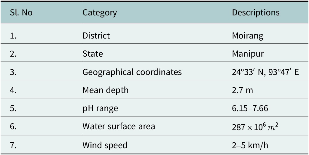
The Northeastern region of India faces a demand–supply deficit of 5.69% in electricity (Sonowal, Reference Sonowal2025), highlighting the need for clean and sustainable power generation solutions. Loktak Lake, located in Moirang, Manipur (24°33′ N, 93°47′ E), is the largest freshwater lake in northeastern India, covering an average area of 287 km2 with a mean depth of 2.7 m and a pH ranging from 6.15 to 7.66. Its size varies seasonally between 250 and 500 km2, with a catchment area of about 980 km2.
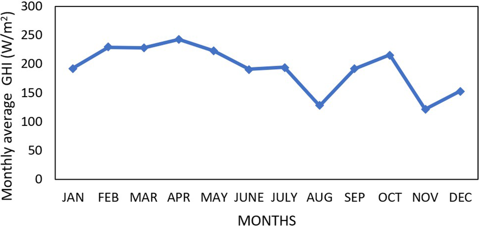
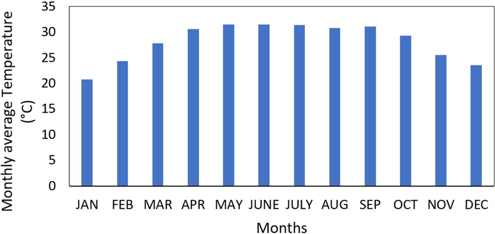
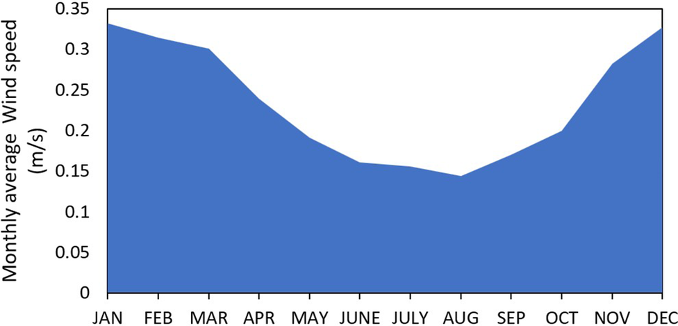
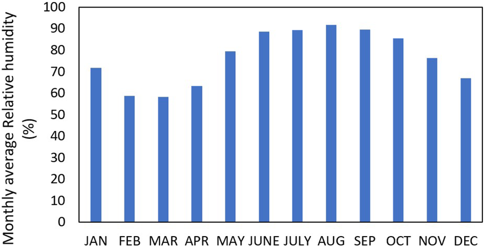
Figures 2–5 represent the annual average data of GHI, temperature, wind speed and relative humidity, respectively, for Loktak Lake in the year 2023. The satellite weather data are taken from the National Solar Radiation Database (National Renewable Energy Laboratory, 2023) and the analysis is performed in SAM.
Monthly average GHI of Loktak Lake for the year 2023.

Monthly average temperature of Loktak Lake for the year 2023.

Monthly average wind speed of Loktak Lake for the year 2023.

Monthly average relative humidity of Loktak Lake for the year 2023.

Loktak Lake exhibits a warm and humid climate favorable for FSPV deployment (Table 1). The average annual temperature is 28.19 °C, with a peak of about 31.5 °C in June and a minimum of 20.8 °C in January. The site records an annual mean relative humidity of 76.65% and an average wind speed of 0.2348 m/s, with the maximum in January. The average annual GHI is 192.75 W/m2, peaking in April before gradually declining through August. The cooler lake surface also helps lower module operating temperatures by 10.8 °C, enabling higher FSPV energy yield compared to land-based systems.
Details of Loktak Lake (Nguyen and Nguyen, Reference Nguyen and Nguyen2015)

Table 1. Long description
The table consists of seven rows of data under the headers Sl. No, Category, and Descriptions.
* Row 1. District. Moirang.
* Row 2. State. Manipur.
* Row 3. Geographical coordinates. 24 degrees 33 minutes North, 93 degrees 47 minutes East.
* Row 4. Mean depth. 2.7 m.
* Row 5. p H range. 6.15 to 7.66.
* Row 6. Water surface area. 287 times 10 super 6 m super 2.
* Row 7. Wind speed. 2 to 5 km forward slash h.
Design and modeling
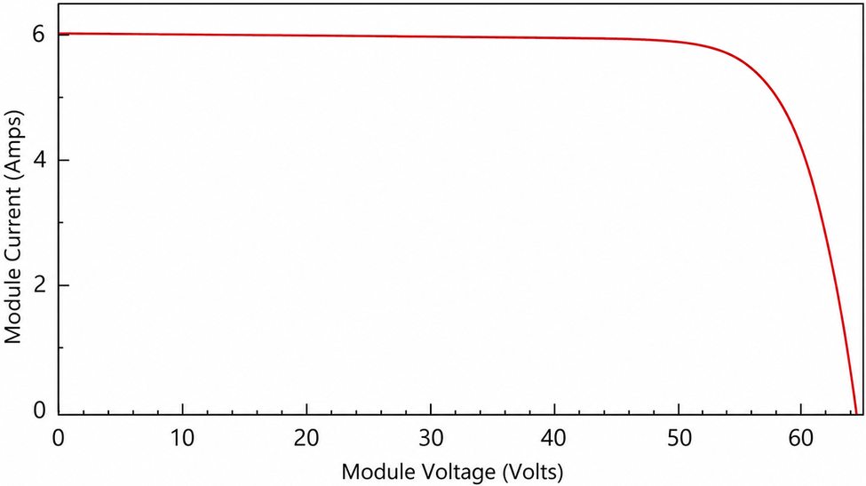
A 13 MW floating solar plant is designed on Loktak Lake using the software called System Advisory Model (SAM). The choice to implement the 13 MW FSPV on Loktak Lake, Manipur, was a well-weighed decision employing considerations about environmental sensitivity, technical feasibility and regional infrastructure limitations. Though the lake could easily support a much larger installation, by keeping the capacity to 13 MW, minimal disruption is caused to the ecology of diverse aquatic fauna. This capability also respects the use of the lake for fishing, along with other community uses, as it covers <1% of the water surface. The system is also appropriately sized to match regional demand and help to supply the electricity demand of Northeast India, thereby minimizing energy curtailment and ensuring efficient utilization of solar resources. Overall, the 13 MW capacity was strategically selected not as a constraint, but as a sustainable and replicable model for clean energy development in ecologically sensitive zones. The PV module used for this is SunPower’s SPR-E19-310-COM. It is made up of single-crystal silicon, mono-facial. The dimensions of this module are 1.559 m in length and 1.046 m in width, making up an area of 1.631 m2. The efficiency of this module is around 19.02%. The open circuit voltage is 64.4 V, and the short circuit current is 6A. This module provides a maximum power output of 310.149 W, with a maximum voltage of 54.7 V and a maximum current of 5.7 A. The temperature coefficient of this module is −0.386%/°C. The total number of cells used is 96. Figure 6 shows the I–V characteristic graph of the solar module as simulated in SAM using Eq. 8.
I–V characteristic graph of the solar module.

Figure 6. Long description
The line graph plots Module Current in Amps on the vertical Y axis against Module Voltage in Volts on the horizontal X axis. The Y axis ranges from 0 to 6 with increments of 2. The X axis ranges from 0 to 60 with increments of 10.
* The red data curve begins at the Y axis intercept at approximately 6 Amps and 0 Volts.
* From 0 to 50 Volts, the current remains nearly constant, forming a horizontal plateau at just under 6 Amps.
* At approximately 50 Volts, the curve reaches a knee point where it begins to bend downward.
* Beyond 55 Volts, the current drops sharply in a steep asymptotic curve, intersecting the X axis at approximately 64 Volts where the current reaches 0.
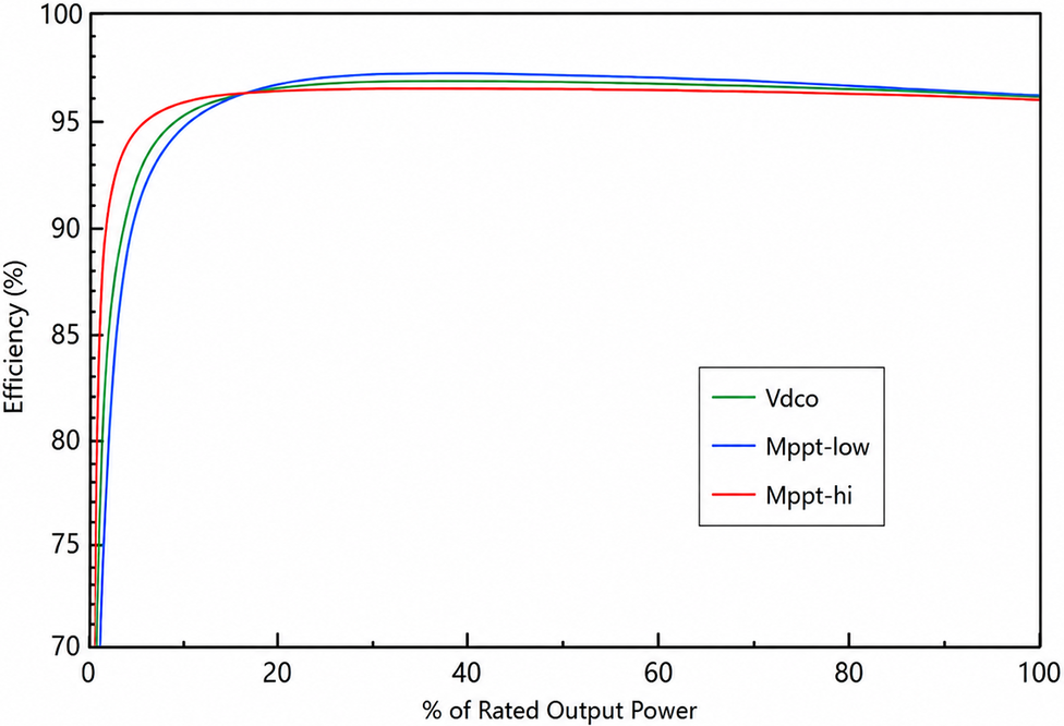
The inverter used for simulation is DYNAPOWER CPS-1500 Gen4 [480 V] with a maximum AC power output of 1.199 MW and a maximum DC power of 1.247 MW. The operational power used is 3922.95 Wdc. The inverter provides a nominal AC voltage of 480 V and a nominal DC voltage of 1000 V. Figure 7 shows the efficiency curve of this inverter. The minimum and maximum MPPT DC voltage are 740 V and 1500 V, respectively.
Efficiency curve of the inverter.

Figure 7. Long description
The X axis represents the percentage of Rated Output Power ranging from 0 to 100. The Y axis represents Efficiency percentage ranging from 70 to 100. Three curves are plotted: V d c o in green, M p p t-low in blue, and M p p t-hi in red.
All three curves show a sharp logarithmic increase from 0 percent power, reaching a plateau between 20 percent and 40 percent power.
* The red curve (M p p t-hi) rises most steeply at low power, peaking at approximately 96.5 percent efficiency around 20 percent power before maintaining a very slight downward slope.
* The green curve (V d c o) has an intermediate rise, peaking at approximately 97 percent efficiency.
* The blue curve (M p p t-low) has the slowest initial rise but reaches the highest peak efficiency of approximately 97.5 percent at 40 percent power.
Beyond 40 percent power, all three curves converge slightly, ending between 96 percent and 96.5 percent efficiency at 100 percent rated output power.
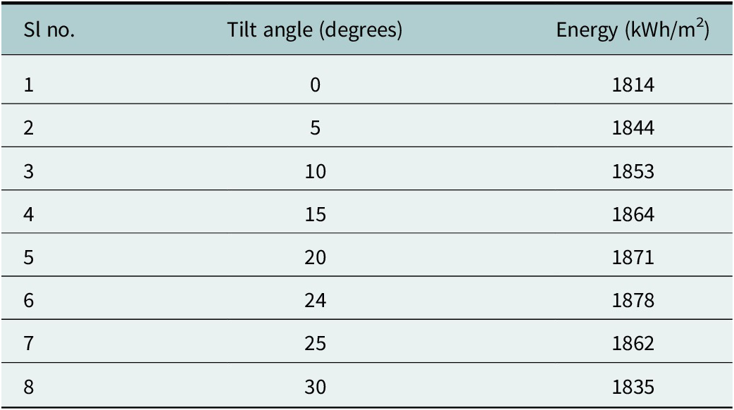
The total area covered by the modules is 68,371.520 m2. The total number of inverters used is 13. The number of modules used is 41,920, and the number of strings is 2096. Total inverter DC capacity is 12,479,400 kW. The DC to AC ratio is kept at 1.10. Considering the civil works and overhead, the total area is taken as 83,276 m2. The floaters used are HDPE pontoon-type floaters having a height of 0.6 m above the water surface to ensure proper cooling of the modules. For designing the FSPV system, when the wind speed is <7 m/s, the angle of tilt should not be <15° (Elshafei et al., Reference Elshafei, Ibrahim, Helmy, Abdallah, Eldeib, Badawy and AbdelRazek2021; National Renewable Energy Laboratory, 2023). Table 2 presents the variation of energy generated with tilt angle for the FSPV system. From Table 2, it is seen that the maximum energy generation is obtained when the tilt angle is the same as the latitude of the location. In this case, the solar panels are tilted by an angle of 24° to provide the maximum output efficiency and reduce drag force; also, the azimuth angle is 180°. The tilt angle is taken as a fixed tilt for both cases.
Variation of energy generation with tilt angle

Table 2. Long description
The table consists of three columns: Sl no., Tilt angle in degrees, and Energy in k W h per m super 2.
* Row 1: 0 degrees yields 1814 k W h per m super 2.
* Row 2: 5 degrees yields 1844 k W h per m super 2.
* Row 3: 10 degrees yields 1853 k W h per m super 2.
* Row 4: 15 degrees yields 1864 k W h per m super 2.
* Row 5: 20 degrees yields 1871 k W h per m super 2.
* Row 6: 24 degrees yields a peak energy of 1878 k W h per m super 2.
* Row 7: 25 degrees shows a decrease to 1862 k W h per m super 2.
* Row 8: 30 degrees shows a further decrease to 1835 k W h per m super 2.
The data indicates that energy generation increases with the tilt angle up to 24 degrees, after which it begins to decline.
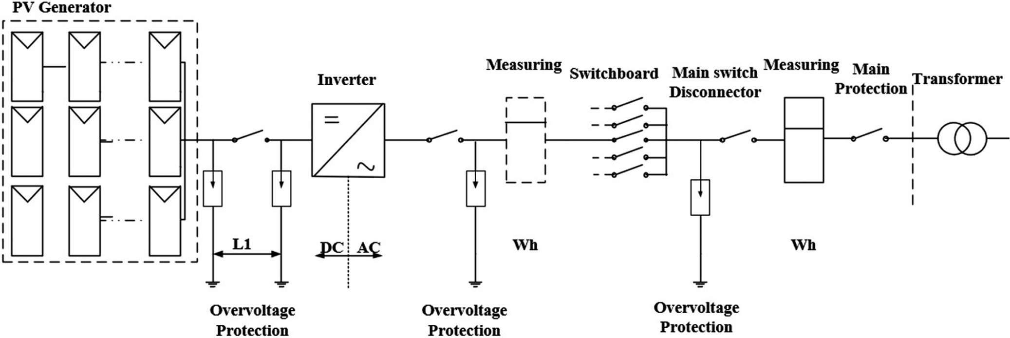
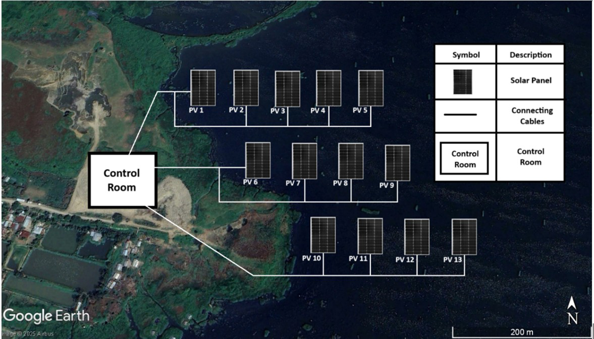
Generally, for areas with low wind speed, the maximum height of the wind-generated wave will be 25 cm (Elshafei et al., Reference Elshafei, Ibrahim, Helmy, Abdallah, Eldeib, Badawy and AbdelRazek2021). To decrease drag, the 13 MW FSPV system is designed to have 1 MW islands on the lake. This will guarantee that the system remains safe even during natural calamities like cyclones. This will also help to increase the reliability of the system, if any issue arises in one island, the other island will operate. The single-line diagram of the 1 MW FSPV island is given in Figure 8. The average area of the Loktak Lake is 287 km2. Here, the FSPV system is designed with a capacity of 13 MW, having a total area of 83,276 m2. The lake coverage by the FSPV system is 0.029% of the total lake area. The schematic diagram of the system is presented in Figure 9.
Schematic diagram of a 1 MW FSPV system.

Figure 8. Long description
The diagram consists of the following components arranged from left to right.
* P V Generator. A dashed box containing a grid of solar panels arranged in three rows and three columns.
* First Overvoltage Protection. A line leads from the generator to a switch, with a grounded protection component labeled L 1.
* Inverter. A square symbol with a diagonal line separating a D C equals sign and an A C tilde wave. A vertical dashed line below it separates the D C and A C zones.
* Second Overvoltage Protection. Following the inverter and another switch, a grounded component is labeled W h.
* Measuring. A dashed rectangular box containing a horizontal line.
* Switchboard. A series of five parallel switches connected to a single output line.
* Main Switch Disconnector. A single switch followed by a third grounded Overvoltage Protection component.
* Measuring and Main Protection. A solid rectangular box labeled W h followed by a final switch.
* Transformer. The circuit terminates at a symbol consisting of two interlocking circles, separated from the previous section by a vertical dashed line.
Schematic diagram of the FSPV system (24°33′13′′ N, 93°47′56′′ E) (Base image © 2025 Airbus, obtained via Google Earth Pro. Map data: Google. Image modified by the authors.).

FSPV systems operate in direct contact with water and are therefore more vulnerable to environmental deterioration. Although modules, cables and inverters are designed as per IEC standards for moisture, salinity, UV exposure, humidity and mechanical stress (Dörenkämper and Arifeen Wahed, Reference Dörenkämper, Wahed, Kumar, de Jong, Kroon and Reindl2021), performance degradation still occurs during long-term outdoor operation. Major failures include hot spots, delamination, snail tracks, corrosion of metallic parts and biofouling from algae and aquatic organisms, all of which reduce system output (Acharya, Reference Acharya2022; Charles Rajesh Kumar and Majid, Reference Charles Rajesh Kumar and Majid2023; Cosgun and Demir, Reference Cosgun and Demir2024). Dust accumulation and bird droppings further restrict module performance, requiring regular cleaning and preventive maintenance. Water quality also plays a significant role, and installations on freshwater bodies generally experience lower corrosion rates. Continuous inspection and maintenance are essential to ensure the reliable operation and extended lifetime of FSPV installations.
Result and discussions
The simulation of a 13 MW FSPV and LBPV power plant has been done successfully with the help of the SAM software. There are two case studies: one without considering the humidity degradation on FSPV and another case study where the humidity-based degradation is considered.
Loss consideration
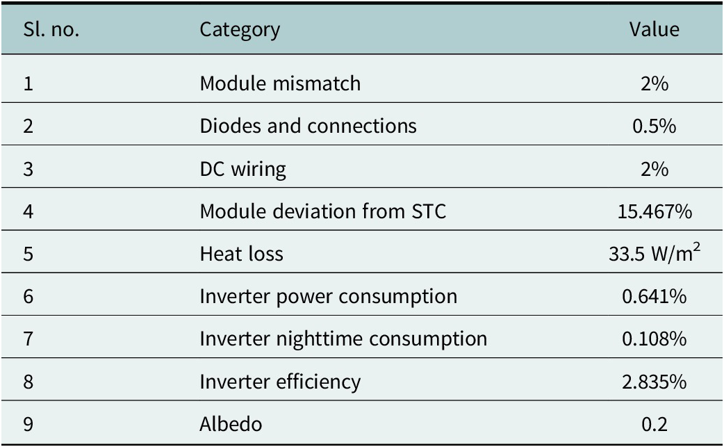
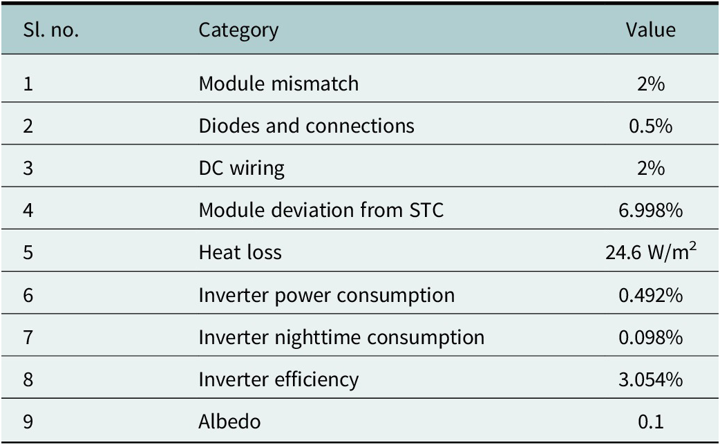
Accurate loss evaluation is essential for realistic performance estimation of both LBPV and FSPV systems. Tables 3 and 4 summarize the modeled losses. Previous literature reports that module mismatch losses are around 2%, while diode and connection losses are ~0.5%. The deviation from STC is higher for LBPV (15.47%) compared to FSPV (6.998%) due to the cooling benefit of water, which reduces module operating temperature and improves efficiency (Acharya and Devraj, Reference Acharya and Devraj2019; Kumar et al., Reference Kumar, Niyaz and Gupta2021). Based on local climatic conditions, the FSPV system is expected to operate at temperatures 12.2°C lower in summer, 9.4°C in monsoon and 7.9°C in winter than LBPV modules, with the greatest benefit observed in peak summer (Haque et al., Reference Haque, Bharath, Khan, Khan and Jaffery2019; Gonzalo et al., Reference Gonzalo, Marugán and Márquez2020). Albedo values of 0.1 for FSPV and 0.2 for LBPV were selected based on the lower reflectivity of water surfaces (Acharya and Devraj, Reference Acharya and Devraj2019; Mavraki et al., Reference Mavraki, Bos, Vlaswinkel, Roos, de Groot, van der Weide, Bittner and Coolen2023). Although SAM simulations may deviate from real plant performance (RMSE of 0.09 for PR and 0.34 for array yield), both systems are modeled uniformly, ensuring a fair comparative analysis. For the LBPV system, the nominal DC generation is 22,415,078 kWh, and after accounting for losses (Table 3), the net delivered AC output is 17,286,254 kWh.
Losses in the LBPV system (Acharya and Devraj, Reference Acharya and Devraj2019; Haque et al., Reference Haque, Bharath, Khan, Khan and Jaffery2019; Gonzalo et al., Reference Gonzalo, Marugán and Márquez2020; Kumar et al., Reference Kumar, Niyaz and Gupta2021; Mavraki et al., Reference Mavraki, Bos, Vlaswinkel, Roos, de Groot, van der Weide, Bittner and Coolen2023)

Table 3. Long description
The table consists of three columns: Sl. no., Category, and Value.
* Module mismatch: 2 percent.
* Diodes and connections: 0.5 percent.
* D C wiring: 2 percent.
* Module deviation from S T C: 15.467 percent.
* Heat loss: 33.5 W per m-squared.
* Inverter power consumption: 0.641 percent.
* Inverter nighttime consumption: 0.108 percent.
* Inverter efficiency: 2.835 percent.
* Albedo: 0.2.
Losses in the FSPV system (Acharya and Devraj, Reference Acharya and Devraj2019; Haque et al., Reference Haque, Bharath, Khan, Khan and Jaffery2019; Gonzalo et al., Reference Gonzalo, Marugán and Márquez2020; Kumar et al., Reference Kumar, Niyaz and Gupta2021; Mavraki et al., Reference Mavraki, Bos, Vlaswinkel, Roos, de Groot, van der Weide, Bittner and Coolen2023)

Table 4. Long description
The table consists of three columns titled Sl. no., Category, and Value. The data rows are as follows.
* Row 1. Category: Module mismatch. Value: 2 percent.
* Row 2. Category: Diodes and connections. Value: 0.5 percent.
* Row 3. Category: D C wiring. Value: 2 percent.
* Row 4. Category: Module deviation from S T C. Value: 6.998 percent.
* Row 5. Category: Heat loss. Value: 24.6 W all over m super 2.
* Row 6. Category: Inverter power consumption. Value: 0.492 percent.
* Row 7. Category: Inverter nighttime consumption. Value: 0.098 percent.
* Row 8. Category: Inverter efficiency. Value: 3.054 percent.
* Row 9. Category: Albedo. Value: 0.1.
The nominal DC electricity generation of the FSPV model is 22,415422 kWh. The losses in the FSPV system are mentioned in Table 4. The calculated net DC electricity generation is found to be 19,920,974 kWh. Considering all the losses, the net AC generation to the grid is 19,005,904 kWh.
Case 1: No degradation
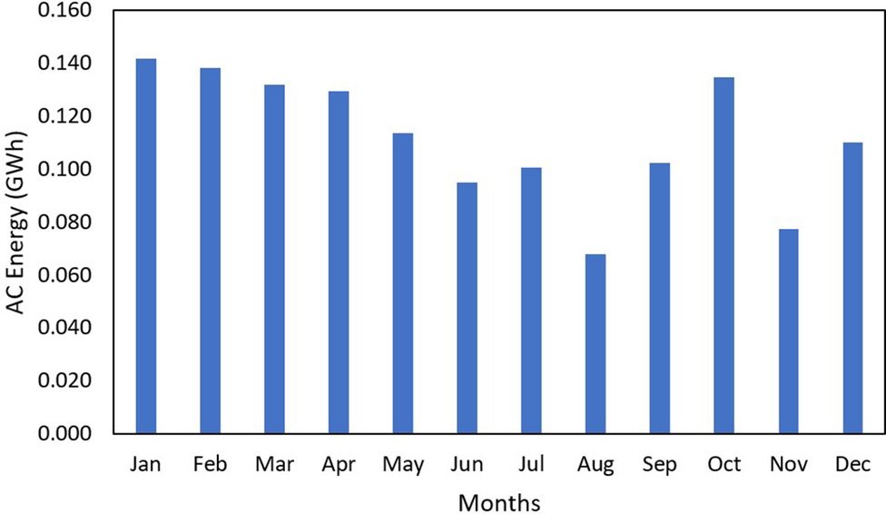
The performance of the FSPV system is first evaluated under ideal operating conditions, excluding humidity-induced degradation. To establish a fair baseline, both LBPV and FSPV systems are assumed to operate at the same relative humidity (76.649%), even though FSPV systems typically experience higher moisture exposure. The monthly AC energy generation for the 1 MW systems is shown in Figure 10, calculated from the irradiance data using Eqs. 14–17.
Monthly cumulative AC generation of 1 MW LBPV system.

The monthly AC energy generation data for the 1 MW LBPV system reveal distinct seasonal variations that reflect the influence of climatic and irradiance patterns across the year. The system recorded an annual energy output of 13.436 MWh, with January (1.418 MWh) and February (1.383 MWh) emerging as the most productive months, contributing ~10.33% and 10.08%, respectively, of the annual yield. These peak performances during the winter months can be attributed to clear sky conditions, lower ambient temperatures and reduced thermal losses, which typically enhance PV module efficiency. Similarly, October (1.349 MWh) also showed high output due to improved irradiance post-monsoon.
In contrast, August exhibited the lowest generation (0.678 MWh), accounting for merely 4.93% of the total annual yield. This dip corresponds with the peak monsoon season in many parts of India, where dense cloud cover and reduced solar insolation significantly hinder generation. Other low-performing months include November (0.773 MWh) and June (0.951 MWh), also affected by either early monsoon conditions or reduced daylight hours. The data highlights a marked generation deficit during the monsoon period (June–August), which cumulatively contributes only 19.2% of the annual energy, underscoring the need for either complementary energy sources or improved storage solutions during this time.
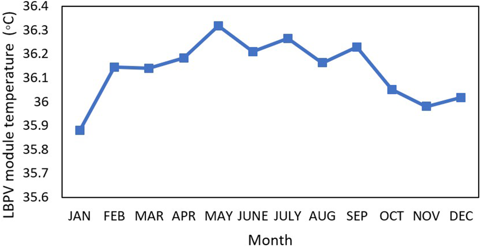
On the other hand, the winter season (December–February) accounts for a surprisingly high 28.4% of the total annual generation, indicating that lower temperatures and higher solar angles contribute positively to PV performance despite shorter days. The pre-monsoon period (March–May) remains moderately productive, generating around 27.3% of the annual yield, while the post-monsoon period (September–November) contributes the remaining 22.9%. The annual AC energy generation of the 13 MW LBPV model is around 17.28 GWh. The average temperature of the LBPV modules over 1 year is around 36.12 °C, and the monthly average temperature of the LBPV modules is given in Figure 11.
Temperature data of a 1 MW LPBV module.

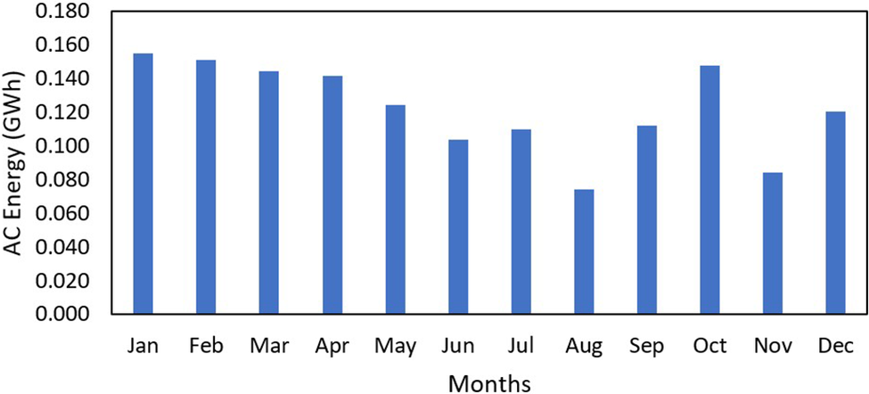
The monthly performance of the 1 MW FSPV plant was analyzed using SAM, resulting in an annual energy output of 1.4708 GWh. Higher generation was recorded in January, February and October, which together contributed 29.5% of the annual output due to lower ambient temperatures and clearer sky conditions. Strong performance was also observed in March (0.1445 GWh) and April (0.1419 GWh), supported by high irradiance and moderate operating temperatures. A slight decline occurred in May (0.1247 GWh) with the onset of higher temperatures and humidity.
Even during the monsoon period, the system maintained stable performance, generating 0.1041 GWh in June, 0.11 GWh in July and 0.0742 GWh in August. Although output dipped in August, the reduction was less severe compared to typical land-based systems, indicating the benefits of the water-based cooling effect. Post-monsoon recovery was noticeable, with September and October producing 0.1122 and 0.1477 GWh, respectively. Moderate generation continued in November (0.0846 GWh) and December (0.1205 GWh).
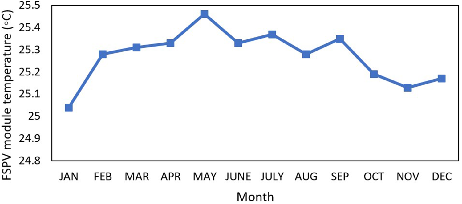
Figure 12 represents the monthly AC electricity generation in year 1. The data are derived from the SAM simulations, which are calculated by Eqs. 14–17. Figure 13 shows the data of the temperature of FSPV modules, and it is observed that the average temperature is around 25.27 °C.
Monthly AC generation of a 1 MW FSPV system.

Temperature data of 1 MW FSPV modules.

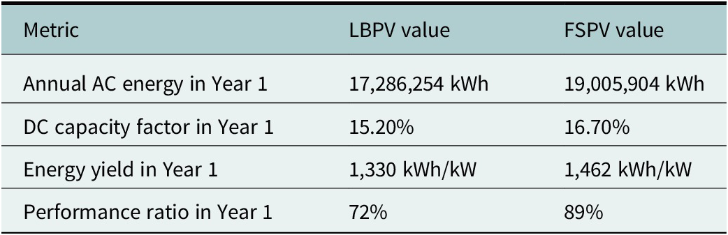
The output results of the 13 MW land-based solar modules and FSPV are depicted in Table 5. The annual AC energy generation of FSPV is higher than that of LBPV. The annual AC generation of FSPV is found to be 19,005,904 kWh, which is 1,719,650 kWh higher than LBPV, which generates 17,286,254 kWh. The annual performance ratio of FSPV is 17% higher than that of LBPV, which has an annual performance ratio of 72%. While the energy yield of LBPV in 1 year is 1,330 kWh/kW, the energy yield in 1 year of FSPV is found to be 1,462 kWh/kW, which is 132 kWh/kW higher.
Performance comparison of the 13 MW LBPV and FSPV systems

Table 5. Long description
The table consists of three columns: Metric, L B P V value, and F S P V value.
* Annual A C energy in Year 1: L B P V is 17,286,254 k W h and F S P V is 19,005,904 k W h.
* D C capacity factor in Year 1: L B P V is 15.20 percent and F S P V is 16.70 percent.
* Energy yield in Year 1: L B P V is 1,330 k W h forward slash k W and F S P V is 1,462 k W h forward slash k W.
* Performance ratio in Year 1: L B P V is 72 percent and F S P V is 89 percent.
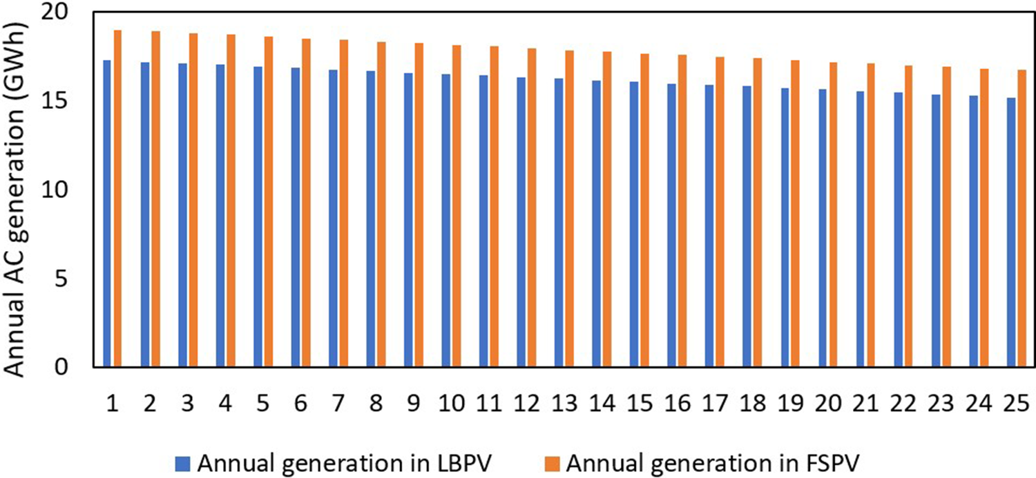
Figure 14 shows the comparison of the net electricity generation of FSPV and land-based solar modules in 25 years of operation. It is clear that the floating solar modules produce more annual electricity than the land-based solar modules.
Comparison between 13 MW LBPV and FSPV annual AC generation.

Figure 14. Long description
The y-axis is labeled Annual A C generation in G W h with a scale from 0 to 20 in increments of 5. The x-axis represents years numbered 1 through 25. A legend at the bottom identifies blue bars as Annual generation in L B P V and orange bars as Annual generation in F S P V.
Throughout the 25 year period, both systems show a gradual linear decrease in energy production. In Year 1, L B P V starts at approximately 17.5 G W h while F S P V starts higher at approximately 19 G W h. By Year 25, L B P V has declined to approximately 15 G W h and F S P V has declined to approximately 16.5 G W h. In every year shown, the orange F S P V bars consistently outperform the blue L B P V bars by a margin of roughly 1.5 to 2 G W h.
Case 2: Water-based degradation
The FSPV system is examined in this scenario in actual environmental conditions, paying particular attention to the impact of humidity. Due to humidity, the FSPV system undergoes degradation effecting the performance. Several studies, including IEC 61215 damp-heat qualification tests and NREL accelerated aging investigations, demonstrate that high relative humidity accelerates moisture-driven degradation mechanisms in PV modules such as metallization corrosion, EVA browning, increased series resistance and loss of fill-factor (Kempe and Wohlgemuth, Reference Kempe and Wohlgemuth2013; Segbefia et al., Reference Segbefia, Imenes and Saetre2021). However, these studies do not directly provide a closed-form equation for converting relative humidity into annual module performance loss. Therefore, in this work, a simplified and conservative humidity degradation model is introduced to translate site-specific humidity conditions into an additional degradation term and given in Eqs. 19–20 (Segbefia et al., Reference Segbefia, Imenes and Saetre2021; Nobre et al., Reference Nobre, Rocha, Healing, Ji, Boulêtreau, Armstrong and Cucherousset2024).

where
$ R{H}_{FSPV} $
 is the relative humidity of the FSPV system,
$ R{H}_{LBPV} $
 is the relative humidity of the location and
α
is the humidity sensitivity coefficient representing the increase in degradation per percentage point of relative humidity (RH) above the threshold.
The effective module efficiency becomes:

where
$ \eta $
 is the efficiency of the system without humidity correction.
For the study location, the average relative humidity is 76.649%. Previous research has shown that FSPV systems typically experience 10–16% higher effective humidity exposure than equivalent land-based systems due to continuous proximity to the water surface and increased moisture retention (Dzamesi et al., Reference Dzamesi, Ahiataku-Togobo, Yakubu, Acheampong, Kwarteng, Samikannu and Azeave2024; Nobre et al., Reference Nobre, Rocha, Healing, Ji, Boulêtreau, Armstrong and Cucherousset2024; Naushad et al., Reference Naushad, Rimon and Khan2025). In this work, the higher end of this range (14% higher RH) is adopted to evaluate a conservative worst-case scenario for the floating system, as the region is tropical and humid, and
$ \alpha $
 is taken as 0.3, as per previous literature (Tripathi et al., Reference Tripathi, Ray, Aruna and Prasad2021; Rajput et al., Reference Rajput, Singh, Singh, Karthick, Shah, Meena and Zahra2024). The resulting adjusted humidity value is then applied in the linear degradation formulation, providing a transparent engineering approximation for incorporating humidity-induced corrosion effects when detailed moisture-transport modeling is not available, while remaining consistent with observed performance degradation trends reported in NREL and IEC 61215 humidity–acceleration results. The humidity degradation, Dh, is applied multiplicatively to the SAM module efficiency to obtain a humidity-corrected (effective) efficiency.
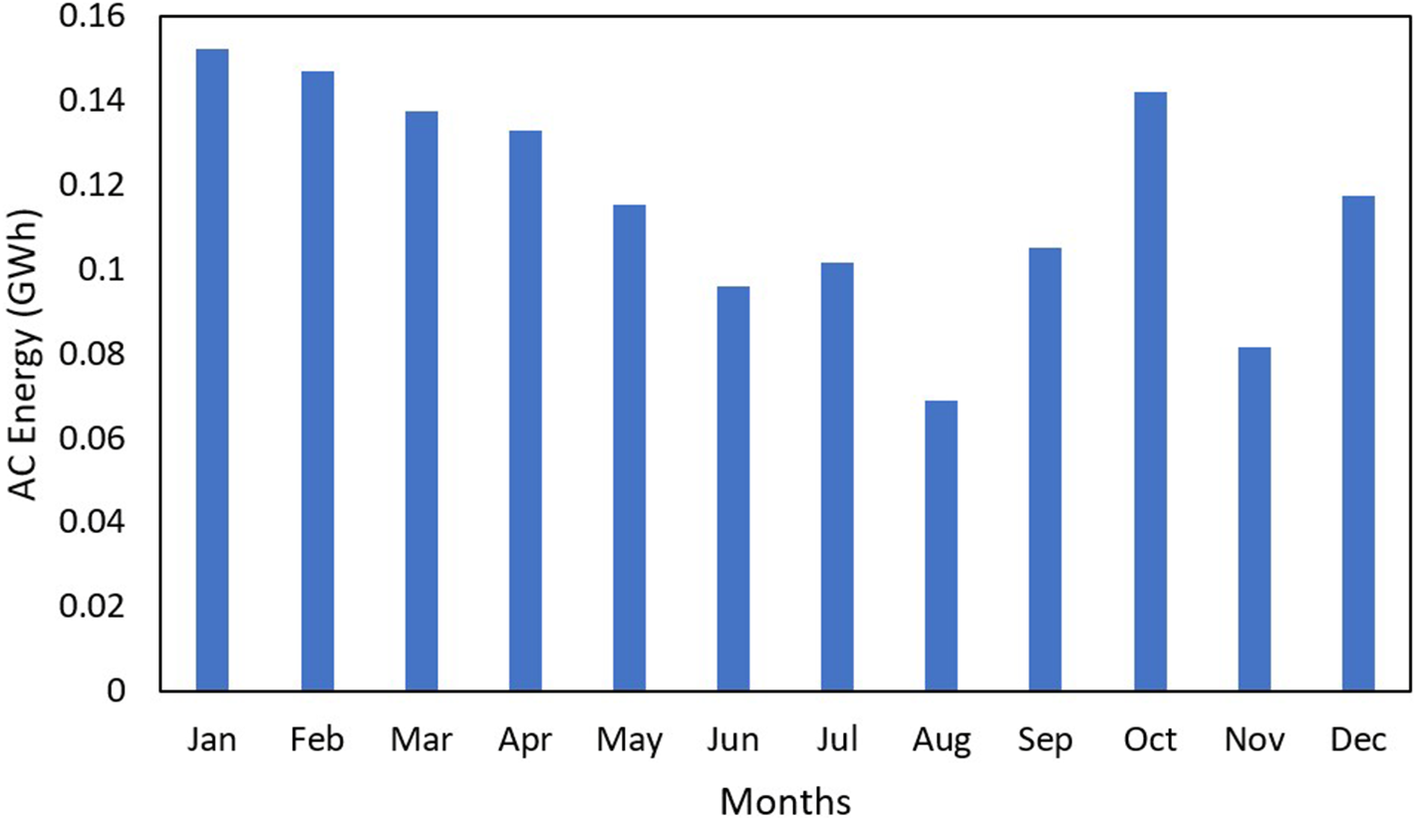
It is seen that after incorporating the humidity-based degradation, the power output of FSPV is affected. Figure 15 shows the data related to the monthly AC generation of the 1 MW FSPV model in year 1 while considering humidity. The monthly values varied between 0.0689 GWh (August) and 0.1523 GWh (January). The data shows the importance of seasonal variation of humidity on the PV module performance, especially during the monsoon and post-monsoon season.
Monthly AC generation of 1 MW FSPV while considering humidity.

Peak generation took place in January (0.1523 GWh) and February (0.1469 GWh), representing 10.51% and 10.14%, respectively, of the annual production. These are months with clear sky, low environmental temperatures and a low level of atmospheric humidity, which contribute to the highest level of efficiency of photovoltaic conversion. Same thing for October (0.1423 GWh) and March (0.1377 GWh): the high values maintained still good performances showing that it is possible to keep the electricity performances good for moderately humid conditions when the irradiance is large enough and the thermal load is low.
The output energy reduces in the summer period (April–June) as humidity and temperature continue to rise. May (0.1154 GWh) and June (0.0962 GWh) have significantly lower than expected high generation potential, which indicates that performance starts to be impacted by rising humidity at the time. Humidity effect becomes more significant in monsoon months (July–August) with energy production decreasing to 0.1015 and 0.0689 GWh per month, respectively. The significant fall in August (providing only 4.76% of annual output) highlights the compounded effect of low solar irradiance (caused by clouds) and overcast sky.
After the monsoon, the performance starts to improve, and September (0.1054 GWh) and October (0.1423 GWh) are better. Nevertheless, residual atmospheric moisture, particularly in November (0.0815 GWh), can still influence the performance by enhancing the particulate loading and prolonging the drying time of the module surface. December (0.1177 GWh) represents a significant increase due to lower RH and a clearer sky. Notwithstanding the observed humidity-related performance losses, the FSPV system performs well compared to the LBPV system, reiterating the FSPV’s viability in wet tropical environments.
In relation to its baseline 13 MW FSPV output, not including humidity (19.059 GWh), the FSPV power decrease of about 4.6% is a noticeable proof of the measurable impact of humidity on the FSPV performance, even in the case of water-cooling. This highlights the significance of incorporating one or a combination of hydrophobic coatings, an optimized cleaning regime and a passive water repellent cover to prevent moisture-related efficiency drops. Still, the FSPV system performed better than the LBPV system.
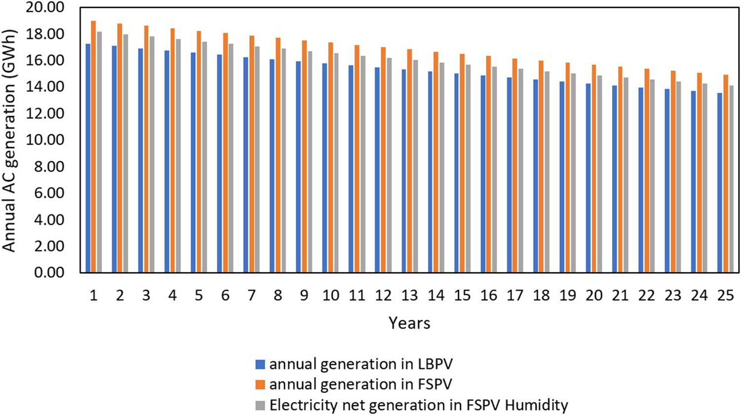
The comparison between the 13 MW LBPV, FSPV and FSPV while considering the effect of humidity is shown in Figure 16.
Annual AC electricity generation of 13 MW LBPV, FSPV and humidity considered FSPV models.

Figure 16. Long description
The vertical Y axis is labeled Annual A C generation in G W h, ranging from 0.00 to 20.00 in increments of 2.00. The horizontal X axis is labeled Years, numbered 1 through 25. Each year contains a cluster of three bars.
* The blue bar represents annual generation in L B P V.
* The orange bar represents annual generation in F S P V.
* The gray bar represents Electricity net generation in F S P V Humidity.
Across all 25 years, the F S P V model (orange) consistently shows the highest generation, starting at approximately 19 G W h in year 1 and declining to about 15 G W h by year 25. The F S P V Humidity model (gray) is the second highest, starting near 18 G W h and ending near 14 G W h. The L B P V model (blue) shows the lowest generation, starting at approximately 17 G W h and ending at approximately 13.5 G W h. All three models exhibit a steady, linear decrease in annual generation over the 25-year period.
Considering the effect of humidity on the FSPV model designed earlier, the annual generation of electricity is found to be 18,192,366 kWh. Although it is less than that of the annual generation of FSPV, it still produces 5.24% higher energy than the LBPV model. Though the output of the FSPV system was higher, the variation of humidity affected the performance of the FSPV system and aided in the corrosion of the system. When calculated over a 25-year operational period, the FSPV system operating under humid conditions results in a cumulative loss of ~23% of the original performance, compared to 21.5% for the LBPV and FSPV systems considering no humidity degradation. This indicates that although the FSPV system initially generates more energy, sustained exposure to waterborne humidity and corrosion mechanisms progressively reduces its long-term advantage unless mitigation strategies, such as enhanced encapsulation, corrosion-resistant materials or improved sealing, are employed. Thus, it is seen that though the FSPV system has higher energy generation, it is also impacted by water-based degradation, which impacts the long-term performance of the system.
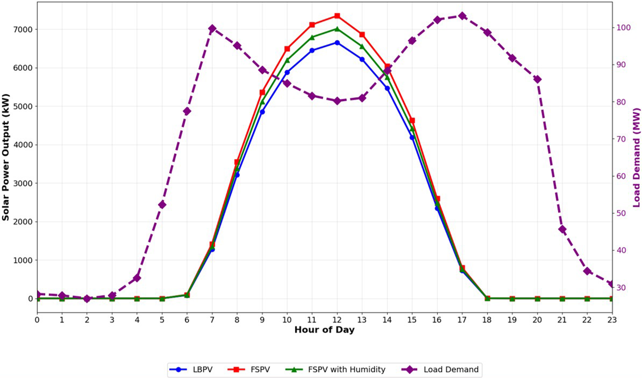
To further illustrate the performance differences among the three systems, an average daily power generation curve was developed by averaging the hourly output over the entire year for the LBPV, FSPV and FSPV with humidity models. This graph is included to visually demonstrate how the systems perform on an hourly basis and how their power production aligns with the regional electricity demand throughout the day. Such a comparison helps assess not only total annual energy generation but also the practicality and operational value of each system in matching real load requirements.
As shown in the Figure 17, both floating systems (FSPV and FSPV with humidity) begin generating electricity shortly after sunrise and reach peak output between 10:00 and 13:00, with the FSPV system showing the highest mid-day generation due to reduced module temperature and enhanced cooling over water. The LBPV system follows a similar profile but consistently produces lower power throughout the day. When humidity-induced degradation is considered, the FSPV with humidity curve remains higher than the LBPV model but demonstrates a clear reduction in peak and total output compared to the ideal FSPV case.
Daily average solar power generation and load demand of the Loktak Lake.

Figure 17. Long description
The X-axis represents the Hour of Day from 0 to 23. The primary Y-axis on the left measures Solar Power Output in k W from 0 to 7000. The secondary Y-axis on the right measures Load Demand in M W from 30 to 100.
Three solid lines represent solar generation, all following a bell curve starting at hour 6, peaking at hour 12, and ending at hour 18.
- F S P V (red line with squares) shows the highest peak at approximately 7300 k W.
- F S P V with Humidity (green line with triangles) peaks at approximately 7000 k W.
- L B P V (blue line with circles) shows the lowest peak at approximately 6600 k W.
A fourth dashed purple line with diamond markers represents Load Demand. It shows a bimodal distribution with two major peaks. The first peak occurs at hour 7 reaching 100 M W, followed by a dip to 80 M W at hour 12. The second peak occurs at hour 17 reaching approximately 103 M W, before declining sharply after hour 21.
When compared against the hourly load demand characteristics of the Loktak region (Northern Regional Load Despatch Centre, 2025; Northern Regional Load Despatch Centre (NERLDC), n.d.), it is evident that the highest regional electricity needs occur during the morning and evening peak periods (06:00–10:00 and 16:00–20:00), whereas PV generation peaks closer to mid-day. The results show that both floating systems (FSPV and FSPV with degradation) generate higher output from ~07:00 to 15:00 h compared to the land-based system. This advantage is due to lower module operating temperatures and better thermal conditions for water. These hours coincide with the rising daytime demand in Loktak, where the load increases sharply from around 05:00 onward. Therefore, the midday peak in FSPV generation allows a greater share of daytime demand to be met directly by solar energy, reducing grid dependence. However, during early morning and late evening hours (before 06:00 and after 17:00), PV output from all systems drops to nearly zero, while the local electricity demand remains between 30 and 100 MW. This mismatch highlights the need for storage or grid support during nonsolar hours. It is important to note that the proposed 13 MW FSPV system is not intended to meet the full regional demand. Rather, the system contributes to reducing the existing demand–supply deficit, particularly during daytime hours when solar availability is highest. By delivering clean and renewable power to the grid during periods of elevated daytime demand, the FSPV installation supports improved grid stability, lowers dependence on conventional thermal generation and contributes to long-term decarbonization objectives.
Lake area coverage
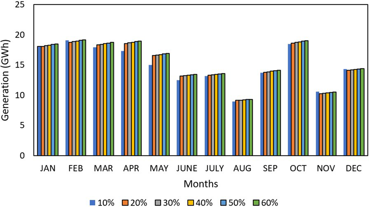
For the current scenario, the lake under examination is Loktak Lake, which is the biggest freshwater lake in South Asia. The average area of the lake is 287 km2. In this article, the FSPV system is designed with a capacity of 13 MW, having a total area of 83,276 m2. This represents only 0.029% of the lake area. To have a better understanding of the effect of the lake coverage area on the performance of the FSPV system, the area of the lake is lowered to make it comparable with the area of the FSPV system. Hence, six cases are considered having lake coverage percentage of 10–60% and shown in Figure 18.
FSPV performance for different lake coverage.

Figure 18. Long description
The vertical Y axis is labeled Generation open parenthesis G W h close parenthesis with a scale from zero to twenty-five in increments of five. The horizontal X axis is labeled Months and lists the twelve months from J A N to D E C. A legend at the bottom identifies six color-coded bars representing lake coverage percentages: ten percent in blue, twenty percent in orange, thirty percent in gray, forty percent in yellow, fifty percent in light blue, and sixty percent in green.
For each month, the bars are clustered together. In most months, there is a slight linear increase in energy generation as the coverage percentage increases from ten to sixty percent. The highest generation occurs in February and October, peaking near twenty G W h. The lowest generation occurs in August and November, dipping below ten G W h. In April and May, the ten percent coverage bar is notably lower than the other five coverage levels, which remain relatively stable compared to each other.
To evaluate the effect of lake coverage on FSPV performance, a parametric approach is adopted in which the effective coverage ratio is varied from 10 to 60%. Since the SAM does not explicitly simulate floating PV systems or coupled water–atmosphere thermal interactions, the influence of coverage is incorporated indirectly through its impact on module operating temperature. Increasing coverage reduces solar radiation incident on the water surface, which lowers the water temperature and enhances the passive cooling effect on PV modules. This reduction in module temperature is reflected in the performance model through adjusted thermal behavior, consistent with observations reported in previous FSPV studies. Therefore, the analysis captures the thermal benefits of increased coverage while maintaining a consistent simulation framework.
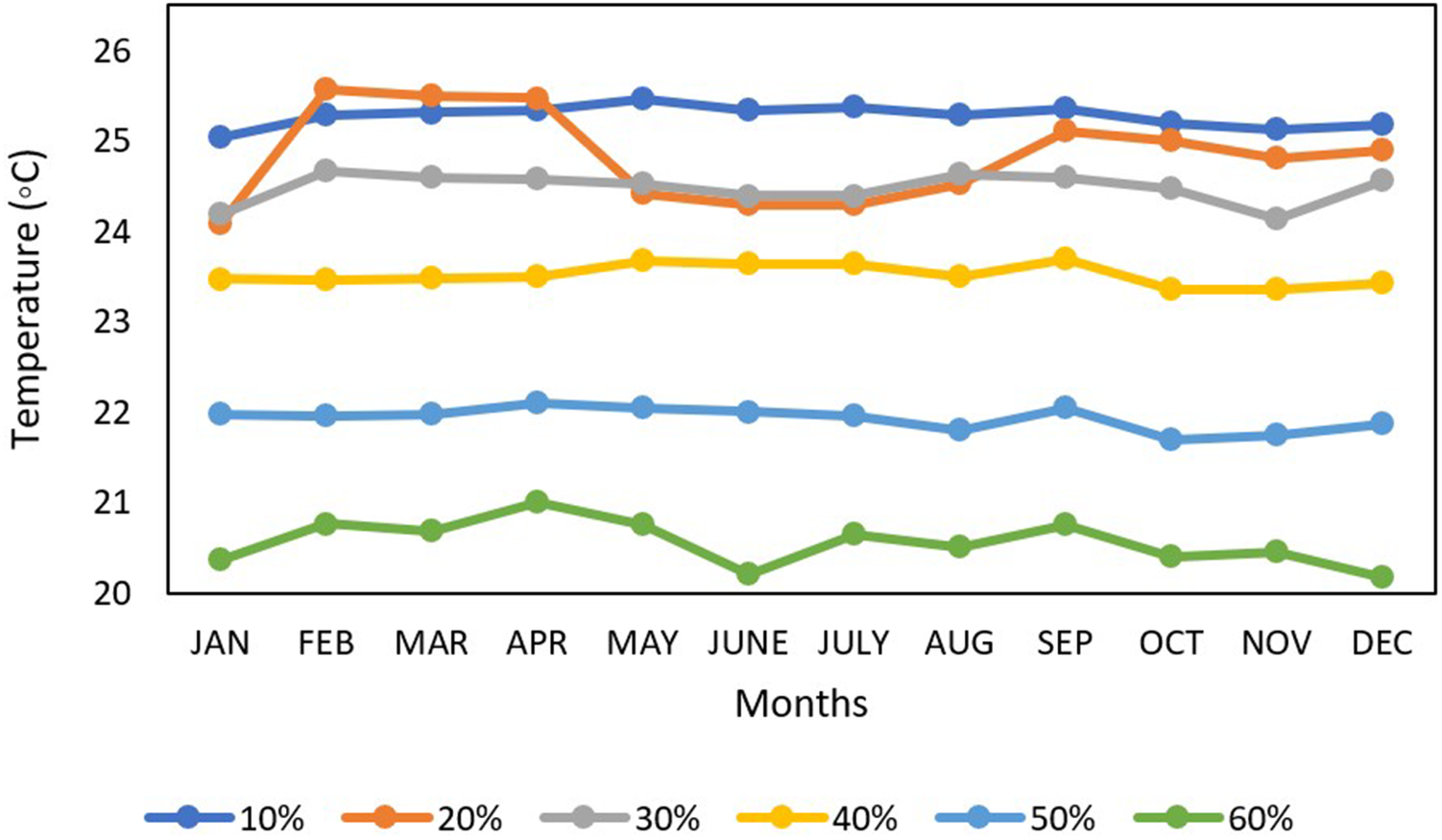
It is seen from Figure 18 that when the lake coverage by the FSPV module is 10%, the average power output is 15.01 GWh, and when the lake coverage is increased to 20%, the FSPV power output increases by 0.41%. Similarly, when the coverage area is increased to 30%, the power output also increases by 0.51%. This happens because with the increase in the lake coverage area, the amount of sunlight reaching the lake decreases, and the temperature of the lake is further lowered, which helps in the increment in the power output of the FSPV system, as shown in Figure 19.
Temperature variation of the FSPV module with the lake coverage area.

Figure 19. Long description
The horizontal x-axis is labeled Months and lists the twelve months from J A N to D E C. The vertical y-axis is labeled Temperature in degrees Celsius and ranges from 20 to 26. Six data series represent lake coverage percentages from 10 percent to 60 percent.
* The 10 percent coverage line in dark blue is the highest, remaining relatively stable between 25 and 25.5 degrees.
* The 20 percent coverage line in orange shows significant fluctuations, peaking at 25.5 degrees in February and March before dropping to 24.3 degrees in June and July.
* The 30 percent coverage line in grey stays mostly between 24 and 24.7 degrees.
* The 40 percent coverage line in yellow maintains a steady path between 23.3 and 23.7 degrees.
* The 50 percent coverage line in light blue follows a lower path between 21.7 and 22.1 degrees.
* The 60 percent coverage line in green is the lowest, fluctuating between 20.2 and 21 degrees.
Overall, as the lake coverage percentage increases, the module temperature decreases across all months.
When the lake coverage is more than 40%, it is observed that the power increment remains nearly constant at 0.55%, and at 60% coverage, there is a slight decrease in the power increment rate, even though the temperature is lower. This effect is interpreted as a consequence of increased module proximity and mutual shading at higher coverage levels.
In general, FSPV systems are designed such that the water coverage is no more than 25–30% of the total water surface (Benjamins et al., Reference Benjamins, Williamson, Billing, Yuan, Collu, Fox, Hobbs, Masden, Cottier-Cook and Wilson2024). Higher coverage hampers the water quality as sunlight cannot reach the majority portions of the water body. This may have an adverse effect on the marine ecosystem by hampering algal growth and affecting water quality (Benjamins et al., Reference Benjamins, Williamson, Billing, Yuan, Collu, Fox, Hobbs, Masden, Cottier-Cook and Wilson2024; Oliveira et al., Reference Oliveira, Almeida and Cardoso2024).
Environmental impact
FSPV systems also help in water conservation. FSPV systems are designed to operate on water covering the water surface, thus lowering evaporation. In India, for areas east of 85° E, the yearly evaporation loss is 1.73 kL/m2 (Central Water Commission, 2017). The 13 MW FSPV system requires an estimated area of 83,276 m2. The overall water savings from minimizing evaporation are 144,067 kL per year. As a result, the plant’s total water usage and water required for cleaning the modules can be balanced. The FSPV system also helps to safeguard the environment by minimizing the carbon dioxide (CO2) impact. Conventional power plants emit a significant amount of CO2 since they utilize coal to generate electricity. In general, coal produces 0.98 kg CO2 for every 1 kWh of energy (Rajput et al., Reference Rajput, Malvoni, Manoj Kumar, Sastry and Jayakumar2020). The yearly CO2 savings from the 13 MW FSPV plant are 13,697 tCO2. The plant will save 342,416 tCO2 throughout its 25-year life. All these further strengthen the FSPV system’s alignment with the SDGs.
Economic analysis
As FSPV systems are designed to work on water bodies, the cost of land is exempted from the capital cost. But FSPV systems require floaters, anchoring and mooring systems. The economic measures are computed using a variety of criteria, in compliance with the rules established by the Indian government. In the Indian scenario, the cost of land is typically taken as 0.325 $/Wp, while the cost of floaters is 0.683 $/Wp (Central Electricity Regulatory Commission, 2016; Nagananthini and Nagavinothini, Reference Nagananthini and Nagavinothini2021; Anusuya and Vijayakumar, Reference Anusuya and Vijayakumar2024). The cost of civil works like roads, drainage and fencing is taken as 0.42 and 0.45 $/Wp for the LBPV and FSPV system, respectively. The electrical cost includes the cost of cables, junction boxes and ancillary equipment, and is taken as 0.35 $/Wp (Central Electricity Regulatory Commission, 2016; Nagananthini and Nagavinothini, Reference Nagananthini and Nagavinothini2021; Anusuya and Vijayakumar, Reference Anusuya and Vijayakumar2024). The standard cost of setting up an LBPV system, including the land cost and module cost in India, is nearly 0.48 $/Wp. The operational cost and cost of ancillaries are higher for the FSPV system and are taken at 0.042 $/Wp, and for the LBPV system, it is 0.038 $/Wp (Anusuya and Vijayakumar, Reference Anusuya and Vijayakumar2024; Goswami and Aizpurua, Reference Goswami and Aizpurua2024). The capital cost for setting up the LBPV system is nearly 1.095 $/Wp. Considering all the economic factors, the cost of the FSPV system is 1.36 $/Wp, which is nearly 21% higher than the LBPV system. The levelized cost of electricity (LCOE) is calculated for both the FSPV and LBPV systems, considering a lifetime of 25 years. For the LCOE calculation, the discount date is taken as 8.7%, contingency as 1.5% of capital cost and inflation rate as 5.3% (da Costa and da Silva, Reference da Costa and da Silva2021; Goswami and Aizpurua, Reference Goswami and Aizpurua2024). The LCOE is calculated using Eq. 21 (da Costa and da Silva, Reference da Costa and da Silva2021).

where
$ \mathrm{CC} $
 represents the capital cost required to set up the system,
$ OA $
 is the cost required for operation,
$ DR $
 is the annual degradation rate and
$ DS $
 is the discount rate.
The payback period (PP) is the amount of time necessary for the total savings and expenses to equal or exceed the initial capital invested and is given in Eq. 22 (da Costa and da Silva, Reference da Costa and da Silva2021).

where
$ cc $
 is the total cost of the system and
$ {c}_{in} $
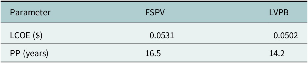
 is the annual cash inflow. The LCOE and payback period calculated for both the LBPV and FSPV systems are given in Table 6.
LCOE comparison between the LBPV and FSPV systems

Table 6. Long description
The table consists of three columns and three rows.
Column headers from left to right are Parameter, F S P V, and L V P B.
Row 1: The Parameter is L C O E in dollars. The value for F S P V is 0.0531 and the value for L V P B is 0.0502.
Row 2: The Parameter is P P in years. The value for F S P V is 16.5 and the value for L V P B is 14.2.
From Table 6, it is seen that the LCOE of the FSPV system is 0.0531 $, while the LCOE of the LBPV system is 0.0502 $. The LCOE of the FSPV system is 5.9% higher than the LBPV system. The LCOE of the FSPV system can be considered comparable to that of the LBPV system, as the FSPV has higher generation. Though financially LBPV systems are favorable presently, FSPV systems provide better adherence to the SDGs. With skyrocketing land prices, soon FSPV will also be a financially viable option, surpassing LBPV systems. India is a highly populated country; industrialization, along with population growth, has led to a surge in land prices. In the last 3 years, the land price in the selected location (Manipur) has risen by 4–5%. The rise in land prices is due to the increase in the state gross domestic product (SGDP). The SGDP has risen by nearly 10–11% in the last 5 years (National Bank for Agriculture and Rural Development (NABARD), 2020-21; Meitei and Sharma, Reference Meitei and Sharma2023). With this rate, within 3–5 years the FSPV system will become a financially viable option for renewable energy generation in the Manipur area.
FSPV systems are a viable, sustainable energy alternative that supports SDG 7. Despite the initial expenditures, FSPV technology offers a revolutionary way to solar power generation that promotes innovation in renewable energy technologies. FSPV systems also support SDG 14 by reducing land-use disputes and conserving maritime environments. Overall, FPV technology is a viable option for attaining sustainable energy and green energy.
Discussion
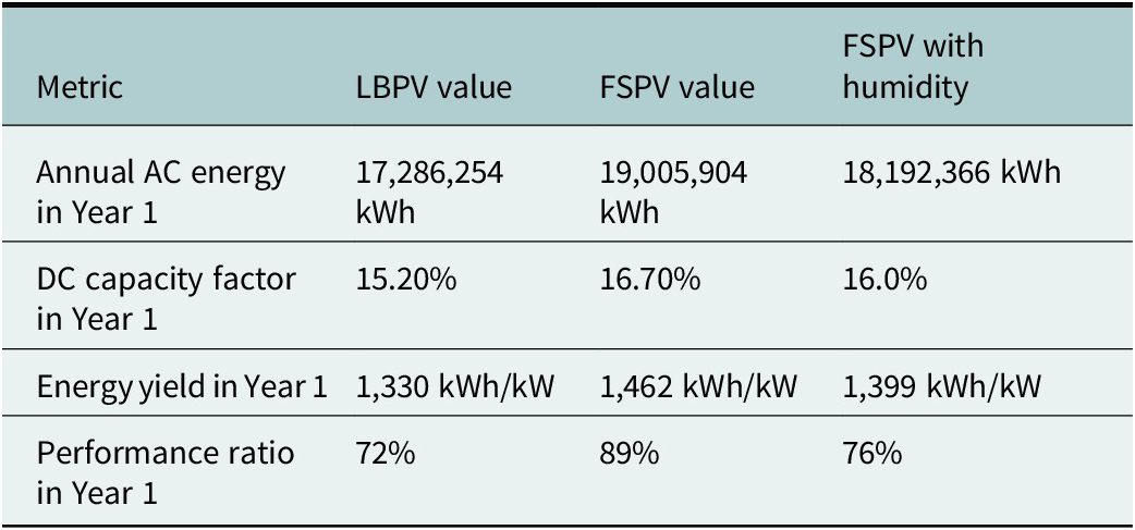
The LBPV power plant is designed in the beginning with the help of SAM software; 17.28 GWh of energy is the annual generation of this model with a DC capacity factor of 15.2% for year 1, and energy yield in year 1 is around 1,330 kWh/kW. The total performance ratio of this model in year 1 is 72%. The major problem with the land-based PV power plant is that it requires a large area of land. India is a very population-dense country, and with the increase in population, the energy needs also increase. Keeping sustainability in mind, the motive is to go eco-friendly; thus, unconventional sources are the best way to meet these rising energy demands. With the abundance of sunlight, solar energy stands out, and in the present scenario, it is one of the major sources of renewable energy. To develop a 13 MW PV power plant, a significant area of land is required. To eliminate the land cost, the FSPV system is developed with floaters where the solar modules float on the surface of lakes, dams and so forth and such water bodies that have a larger water surface area. Therefore, a FSPV system is designed with the help of SAM software. The annual energy generation is found to be 19.05 GWh, which is 9.8% higher than the LBPV model. With a DC capacity factor of 16.7% for the year 1, 1,462 kWh/kW is the year 1 energy yield. The performance ratio of this model was 89% in year 1. The effect of humidity on FSPV is considered, and another model is designed in the SAM software. Table 7 shows the comparison between all three models.
Comparison between the designed systems

Table 7. Long description
The table consists of four columns and five rows. The columns are labeled Metric, L B P V value, F S P V value, and F S P V with humidity.
Row 1: Annual A C energy in Year 1. L B P V is 17,286,254 k W h. F S P V is 19,005,904 k W h. F S P V with humidity is 18,192,366 k W h.
Row 2: D C capacity factor in Year 1. L B P V is 15.20 percent. F S P V is 16.70 percent. F S P V with humidity is 16.0 percent.
Row 3: Energy yield in Year 1. L B P V is 1,330 k W h per k W. F S P V is 1,462 k W h per k W. F S P V with humidity is 1,399 k W h per k W.
Row 4: Performance ratio in Year 1. L B P V is 72 percent. F S P V is 89 percent. F S P V with humidity is 76 percent.
The corrosion caused by the humidity results in degradation of the FSPV modules, which decreases the lifespan of these modules. The humidity factor causes the FSPV modules to corrode, which damages the solar modules. The power output is also affected negatively; the annual AC generation is around 18.19 GWh. The energy yield decreases for the FSPV system when humidity-based corrosion is considered. Similarly, the PR is also reduced for the FSPV system with humidity considerations due to higher losses. The energy yield refers to the actual electricity produced by that system over a given period. PR is the percentage of available energy that is actually converted into electricity, as given in Eqs. 14–17. Hence, a higher performance ratio means that a larger proportion of the available energy is used, although the total energy yield could be lower because of location and weather conditions.
However, the FSPV system still produces higher energy than that of the LBPV system even after considering the corrosion effect due to humidity. Although the FSPV model is producing higher energy, in practical applications, the humidity factor should be considered. After including the corrosion due to humidity, the FSPV model still produces significantly higher energy than that of LBPV. The FSPV system also has environmental benefits as it saves 13,679 tCO2 and also helps to save 144,067 kL of water annually, thus aligning with the aims of SDGs.
Conclusion
This article presents a comparative performance analysis of the performance study of 13 MW FSPV and 13 MW LBPV systems on the Loktak Lake. The novelty of this research lies in its dual-case simulation approach, which uniquely incorporates the effect of humidity-induced corrosion on FSPV performance. This article discusses two case studies: one without considering the increased humidity effect on the FSPV model and another case study where the humidity factor is considered in the FSPV model. Comparison between the LBPV model and the FSPV model (without humidity) is studied in case study 1. In the simulation of the land-based PV system, the annual AC generation was found to be 17.28 GWh. The FSPV system generates an AC energy of 19.05 GWh, which is 9.9% higher energy generation than the LBPV model. The performance ratio of the FSPV system is 89%, and the performance ratio of the LBPV system is 72%.
In case study 2, the higher corrosion due to humidity is considered in the case of the FSPV system. In the FSPV model, the solar modules are floated on the surface of the water body. It is very advantageous as the water helps cool down the surface temperature of the solar modules and increases the power output of the system. However, the humid environment also accounts for corrosion of the floater mechanism and the solar module in general, decreasing the longevity of the solar panels. More research has to be done to select proper materials for the floater mechanism, which will degrade more slowly in such a humid environment. Although humidity affects FSPV negatively, the annual power generation of FSPV is still higher than that of LBPV, with an annual AC generation of 18.19 GWh. This is 5.24% higher energy generation than the LBPV model.
FSPV is becoming increasingly competitive with land-based PV systems with advanced technologies and economic viability. The FSPV model is generating nearly 5.24% higher power output than the LBPV system, even after considering the corrosion effect on the FSPV system. The study contributes a novel methodology for evaluating long-term performance degradation due to humidity and supports global clean energy goals, particularly SDG 7, by demonstrating that FSPV systems can deliver reliable, sustainable and efficient energy in land-constrained and ecologically sensitive regions.
Nomenclature
A. Symbols.

Table A1. Long description
The table contains 47 rows of technical symbols and their corresponding descriptions. Key entries include:
* R sub s e: Resistance in series in ohms.
* R sub t: Shunt resistance in ohms.
* I sub s: Output current of the solar cell in Amperes.
* I sub s m: Photocurrent in Amperes.
* I sub t: Current through shunt resistance in Amperes.
* I sub p n: Current through the diode in Amperes.
* I sub r s: Diode reverse saturation current in Amperes.
* V sub t h: Thermal voltage of P V cell in Volts.
* n: Ideality factor.
* V sub s: Output voltage of the P V cell in Volts.
* X: Number of series connected cells in P V module.
* K: Boltzmann constant 1.380649 times 10 super negative 23 Joules per Kelvin.
* q: Charge on an electron 1.602 times 10 super negative 19 Coulombs.
* T: Temperature in Kelvin.
* I sub m s: Maximum output current of P V cell in Amperes.
* V sub m: Maximum output voltage of the P V cell in Volts.
* T sub i: Operating cell temperature.
* G: Irradiance in Watts per meter-squared.
* V sub s open parenthesis T sub i comma G close parenthesis: Voltage at an operating cell temperature and irradiance.
* C sub v: Temperature coefficient of voltage.
* I sub s open parenthesis T sub i comma G close parenthesis: Current at an operating cell temperature and irradiance.
* C sub i: Temperature coefficient of current.
* T sub S T C: Temperature at S T C in Kelvin.
* G sub S T C: Irradiance at S T C in Watts per meter-squared.
* P sub m s open parenthesis T sub i comma G close parenthesis: Maximum power output at an operating cell temperature and irradiance in Watts.
* P sub c: Power generation capacity of P V in Watts.
* varepsilon: Efficiency of solar modules.
* A sub r e a l: Useful module area in meters-squared.
* P sub s: Output power of solar array in Watts.
* n: Number of solar modules.
* varepsilon sub s: Rated solar module efficiency.
* varepsilon sub i n v: Rated efficiency of inverter.
* A sub m: Area of single module in meters-squared.
* T sub m: Temperature of module in Kelvin.
* Theta sub p: Temperature coefficient of power.
* Y sub E: Energy yield in Watt-hours per Watt-peak per day.
* E sub A: Energy generation in one year in kilo-Watt-hours.
* P sub c a p: Installed capacity of the P V system in kilo-Watts.
* Y sub f i: Final yield in kilo-Watt-hours.
* Y sub r e f: Reference yield.
* E sub a c: Total A C energy output in kilo-Watt-hours.
* E sub L: Incident solar irradiance on the solar panel in kilo-Watt-hours per meter-squared.
* E sub T A: Total energy supplied by the P V plant in one year in Mega-Watt-hours.
* C sub i n: Annual cash inflow.
B. Abbreviations.

Table B1. Long description
The table is organized into two columns: Abbreviation and Description.
* C C: Capital cost
* C U F: Capacity utilization factor
* C U I: Corrosion under insulation
* D R: Degradation rate
* D S: Discount rate
* F S P V: Floating solar photovoltaic
* G H I: Global horizontal irradiance
* H D P E: High-density polyethylene
* I E C: International Electrotechnical Commission
* K C L: Kirchoff’s current law
* L B P V: Land-based photovoltaic
* L C O E: Levelized cost of electricity
* M P P: Maximum power point
* M P P T: Maximum power point tracking
* N S R D B: National solar radiation database
* O A: Operational cost
* O C: Open circuit
* P P: Payback period
* P R: Performance ratio
* P V: Photovoltaic
* R M S E: Root mean square error
* SAM: System advisor model
* S C: Short circuit
* S D G: Sustainable development goal
* S D M: Single diode model
* S G D P: State gross domestic product
* S T C: Standard test conditions
* U N: United Nations
Open peer review
To view the open peer review materials for this article, please visit https://doi.org/10.1017/etr.2026.10016.
Data availability statement
No primary data were generated or required for the present study. Relevant meteorological data referenced in the analysis is publicly available from the National Solar Radiation Database (NSRDB) at https://nsrdb.nrel.gov/.
Author contribution
C.S.S.: Conceptualization, methodology, data curation, software and writing – original draft preparation. A.G.: Supervision, conceptualization, writing – review and editing and corresponding author. A.K.: Methodology, validation and technical review. K.K.: Data analysis, visualization and writing – review and editing. S.B.: Corrosion assessment, environmental impact analysis and validation. S.G.: Literature review, data interpretation and writing – review and editing.
Financial support
The author did not receive any financial support.
Competing interests
The authors declare that they have no known competing financial interests or personal relationships that could have appeared to influence the work reported in this article.
Declaration of generative AI use in scientific writing
During the preparation of this manuscript, the author(s) utilized ChatGPT and Google Gemini to improve grammar and readability. Following the use of this tool, the author(s) carefully reviewed and revised the content as necessary and accept full responsibility for the final version of the manuscript.

 Open access


Comments
From,
Dr. Anik Goswami
Vellore Institute of Technology, Chennai
Chennai- 600127, India.
18th February, 2026.
Dear Editor,
We would like to submit an original research article by Chada Sai Sravan, Anik Goswami, Anand Kumar, Krishna Kumba, Sanjay Bhadra, Soham Ghosh entitled “Floating solar systems for clean energy: Addressing Humidity-Induced Corrosions” to your esteemed journal ‘Energy Transitions’ for consideration and evaluation.
Floating solar photovoltaics (FSPV) is an emerging technology which provides a viable solution for renewable energy generation. With the increasing energy demand all over the world, and depletion of natural resources such as coal and crude oil, it is highly crucial to implement better renewable sources of energy. The implementation of traditional land-based PV power plant system is often hindered by the land acquisition cost. The FSPV system irradicates the land acquisition cost by efficient utilization of surface area of water bodies. The PV modules are floated on the water bodies, the surface of the water body helps maintain the PV module temperature and increasing the overall efficiency, satisfying the aims of SDG 7. This research paper aims to compare the power output of FSPV system and land based PV (LBPV) system, and two case studies are discussed, one without considering the water based corrosive effect on FSPV and another case study where the water based corrosive effect is considered. FSPV systems are emerging as sustainable and ecologically friendly energy sources, in line with SDG 7’s aim of ensuring universal access to cheap, dependable, sustainable, and contemporary energy.
It is of interest to the readers of your journal as FSPV are gaining importance nowadays. The paper focuses on determination of degradation of FSPV modules and analyze the effects of degradation in technical and economic assessment of large scale FSPV power plant.
The authors declare no conflict of interest.
Please address all correspondence concerning this manuscript to me at:
anik91_go@rediffmail.com, anik.goswami@vit.ac.in
We affirm that this manuscript is original, has not been published before and is not currently being considered for publication elsewhere.
Thank you very much for your attention to our paper.
Thanking you,
Anik Goswami
Email: anik.goswami@vit.ac.in
Phone: +91 8777383221