Introduction
The famous Young's equation[Reference Young1] predicts the apparent equilibrium (static) contact angle for a liquid droplet sitting on a smooth, flat solid surface, which is called the Young's angle, θ Y. If the surface has either random roughness or structured patterns, the apparent equilibrium contact angle, θ ap, can be determined using the Wenzel[Reference Wenzel2] or Cassie–Baxter[Reference Cassie and Baxter3] equations. However, the dynamic contact angle and its evolution cannot be predicted using the Young, Wenzel, or Cassie–Baxter equations. The difficulties in modeling dynamic contact angles mainly arise from the singular flow geometry at the contact line of the three phases: liquid, gas, and solid.[Reference Huh and Scriven4] When the pairwise surface tension forces are largely unbalanced near the contact line, the classic no-slip boundary condition becomes invalid in the nearby region; thus, driven by the surface tension force, the contact line starts to move until a new balanced state is reached. Based on this concept, physical and mathematical models can be derived to capture the contact line dynamics.
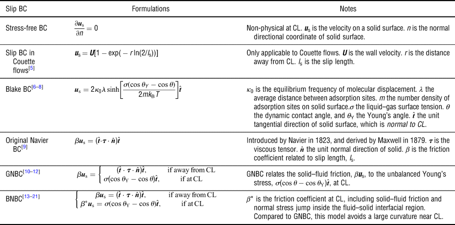
Table I lists a summary of slip boundary models developed for the continuum approach in the literature.[Reference Thompson and Robbins5–Reference Zhang and Ren21] Among these models, a generalized Navier boundary condition (GNBC) proposed by Qian et al.[Reference Qian, Wu, Lei, Wang and Sheng10–Reference Yamamoto, Higashida, Tanaka, Wakimoto, Ito and Katoh12] and a balanced-force Navier boundary condition (BNBC) proposed by Ren and E[Reference Ren and E13–Reference Zhang and Ren21] were independently constructed, and both are based on molecular dynamics results. The GNBC and BNBC capture the dynamic contact angle using the unbalanced Young's stress, σ(cos θ − cos θ Y), where σ is the liquid–gas surface tension, θ Y is the Young's angle, and θ is the dynamic contact angle. The GNBC uses only one friction coefficient, β, while the BNBC uses three friction coefficients, i.e., β L in the liquid–solid contact surface, β G in the gas–solid contact surface, and β* on the tri-phase contact line. Thus, the BNBC is expected to yield more accurate predictions. However, measuring these friction coefficients is difficult, and these coefficients are not yet available in the literature for real materials. Moreover, the relations between the slip velocity and unbalanced stress proposed in GNBC and BNBC are approximate, not constitutional, and have not yet been validated through experiments.
Summary of slip boundary conditions developed in the literature.

CL stands for “contact line”.
There have also been significant developments in the particle methods. The lattice Boltzmann (LB) methods model the solid–surface interactions directly as the pairwise interactions between wall and fluid particles.[Reference Martys and Chen22–Reference Fernandes, Vainstein and Brito24] Limitations and challenges in LB are: (1) spurious interfacial flows strongly influence the contact line motion, and (2) realistic density and viscosity ratios between liquid and gas are not practical.[Reference Chen, Kang, Mu, He and Tao23] Efforts are still in progress to overcome these limitations in LB.[Reference Yu and Fan25] A smoothed particle hydrodynamics model uses a combination of short-range repulsive and long-range attractive interactions between solid–liquid, solid–gas, and liquid–gas particles to simulate the contact angle.[Reference Tartakovsky and Meakin26] A dissipative particle dynamics (DPD) model uses only the short-range repulsive interactions to simulate the contact angle.[Reference Kong and Yang27] In general, the particle methods do not need to explicitly define a slip boundary condition on the contact line. Instead, the slip condition can be captured in particle methods as presented in a DPD work.[Reference Kasiteropoulou, Karakasidis and Liakopoulos28]
In this work, the continuum approach is used to investigate the wetting on micro-patterned surfaces. Micro-patterned surfaces were reported were reported to promote dropwise condensation for heterogeneous wetting behaviors.[Reference Yao, Garvin, Alvarado, Jacobi, Jones and Marsh29] However, little insight into the role of surface morphology on droplet dynamics was provided.
To understand the contact line dynamics on the micro-patterned surfaces, an experimentally validated, constitutional slip boundary model based on the Navier–Stokes (N–S) equations is developed in this paper. Note that our new model does not require fitting parameters, and the model is validated through studying a water droplet interacting with different micropillared substrates under different conditions; i.e., static, receding, and advancing modes. The paper is organized as follows. The physical problem, governing equations, and numerical methods are presented in Section “Physical problem, governing equations, and numerical methods”. The results and analysis are presented in Section “Simulation results and analysis”. Finally, the conclusions are presented in Section “Concluding remarks”.
Physical problem, governing equations, and numerical methods
Physical problem
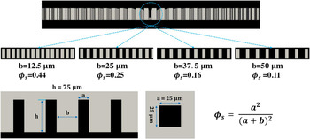
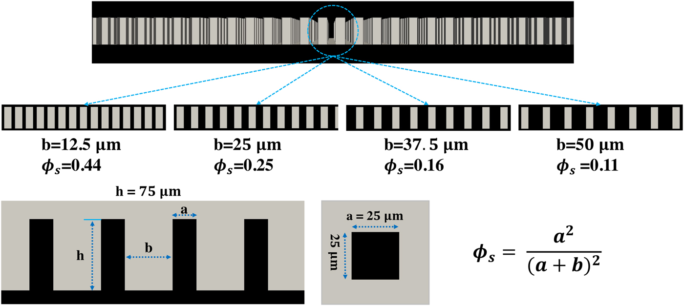
The geometry of the micro-patterned substrates studied in this paper is shown in Fig. 1. Each substrate is covered by a square array of micrometer-sized square pillars. The pillar dimensions are 25 µm × 25 µm × 75 µm. Four substrates with the same pillar dimensions, but different pillar spacings are studied, i.e., 12.5, 25, 37.5, and 50 µm. The area fraction of the liquid–gas interface occluded by the pillars, which is defined as ϕ s in Eq. (1), is used to refer to the four substrates throughout the paper:
 $$\phi _{\rm s} = \displaystyle{{a^2} \over {{(a + b)}^2}} $$
where a is the width of the pillar and b is the spacing between two neighboring pillars. Based on the Cassie–Baxter theory,[Reference Cassie and Baxter3] decreasing ϕ s will increase the hydrophobicity, unless the Wenzel state is reached. Note that all the cases studied in this paper are in the Cassie–Baxter state.
Schematic of the micrometer-sized patterns with square pillars studied in this paper.
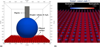
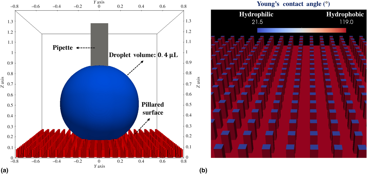
As shown in Fig. 2(a), a 0.4 µL water droplet interacting with the micro-patterned substrates is studied numerically and compared with experiments.[Reference Yao, Garvin, Alvarado, Jacobi, Jones and Marsh29] All simulations in this paper use the same configurations stated as follows. The computational domain is 1.6 mm × 1.6 mm × 1.4 mm, the minimum grid size is Δx = 6.25 μm, and the total number of computational cells is over 8 million. A square micropipette, whose dimensions are 0.2 mm × 0.2 mm × 0.9 mm, is used in the advancing and receding simulations, while it is omitted in the equilibrium simulations. The micro-patterned surface consisting of a micropillar array of hydrophobic and hydrophilic sites is shown in Fig. 2(b). The pillar top-surface is hydrophilic (θ Y = 21.5°), while the side-surfaces and substrate bottom are hydrophobic (θ Y = 119°). This configuration is set according to the experiments.[Reference Yao, Garvin, Alvarado, Jacobi, Jones and Marsh29] Although a large droplet (5–50 µL) was used in the experiments, our numerical simulations cannot handle such large droplets because the pillar size constrains the domain size. Fortunately, our simulation results of a 0.4 µL water droplet agree well with experiments of 5–50 µL droplets. Indeed, it is well accepted that the droplet size does not affect the static and dynamic contact angles.
Simulation configurations: (a) the computational domain (axis unit is millimeter) contains a 0.4 µL water droplet (blue), a micropipette (gray), and a micro-patterned substrate (red); and (b) the Young's angle of the micro-patterned substrate is 21.5° on the pillar top-surface (blue), and 119° on the pillar side surfaces and substrate bottom (red).
Governing equations
The problem described in this section is an incompressible Newtonian, two-phase flow, which is governed by the incompressible continuum equation, and N–S equations:
 $$\nabla \cdot {\bi u} = 0$$
 $$\displaystyle{{\partial \rho {\bi u}} \over {\partial t}} + \nabla \cdot (\rho {\bi uu}) = -\nabla p + \nabla \cdot {\bi \tau} + {\bi F}_{{\rm ff}} + {\rm \;} \rho {\bi g}$$
where u is the flow velocity, ρ the density, t the time, p the pressure,  ${\bi \tau} = \mu \lsqb {\nabla {\bi u} + {\lpar {\nabla {\bi u}} \rpar }^{\rm T}} \rsqb $ the fluid stress tensor, g the gravitational acceleration, and Fff the smeared liquid–gas surface tension force.
A constitutional slip boundary condition for contact line
To capture the contact line motion, a constitutional slip boundary model based on the N–S equations is proposed in this paper:
 $$\eqalign{\rho \left[ {\displaystyle{{\partial u_{\rm s}} \over {\partial t}} + u_{\rm s}{\hat {\bi t}}\cdot \nabla u_{\rm s}} \right] & = \mu _{\rm s}\nabla _{\rm n}^2 u_{\rm s} \cr & + \lsqb {{\hat {\bi t}}\cdot {\bi \tau} \cdot {\hat {\bi n}} + \sigma \lpar {{\rm cos}\,\theta_{\rm Y}-{\rm cos}\,\theta} \rpar \delta_{\rm c}} \rsqb \delta _{\rm s} + \rho g_t} $$
where u s is the slip velocity of the contact line, whose direction is  ${\hat {\bi t}}$, the normal direction of the contact line pointing from liquid to gas (meanwhile,
 ${\hat {\bi t}}$ is tangential to the solid surface), μ s is the liquid viscosity near the solid surface,
 $\nabla _n^2 u_{\rm s} = \nabla ^2u_{\rm s}-{\hat {\bi n}}\cdot \nabla \lpar {{\hat {\bi n}}\cdot \nabla u_{\rm s}} \rpar $ is the 2-D Laplacian operator on the solid surface,
 ${\hat {\bi n}}$ is the normal direction of the solid surface, δ c is a numerical delta function to describe the contact line, δ s is a numerical delta function to describe the solid surface, and
 $g_t = {\bi g}\cdot {\hat {\bi t}}$ is the gravitational acceleration in the direction of
 ${\hat {\bi t}}$.
Equation (4) is a one-dimensional N–S equation written in the direction of  ${\hat {\bi t}}$. The pressure gradient is neglected, because it is expected to be small. Although there is a sharp pressure jump across the contact line due to surface tension, the pressure gradient on either side of the contact line is small. Equation (4) is used in the region near the contact line (δ c > 0), while the classic no-slip condition is used elsewhere (δ c = 0) on the solid surface. Note that although the gravity term, ρg t, is included here, it is negligible based on a simple scale analysis, because the thickness of a contact line is infinitesimal.
There are two dissipation terms working as the damping mechanism: (1) a bulk fluid viscous term,  ${\hat {\bi t}}\cdot {\bi \tau} \cdot {\hat {\bi n}}\delta _{\rm s}$, and (2) a fluid–solid interfacial viscous term,
 $\mu _{\rm s}\nabla _n^2 u_{\rm s}$. The first one is exerted from the bulk fluid, and its viscosity is, of course, the fluid viscosity, μ [see Eq. (9)]. The second one is the viscous dissipation on the contact line, but its viscosity is not yet clear to us. It is commonly recognized that fluid viscosity increases when it meets a solid surface. We use μ s = 10μ L for all cases in this paper (μ L is the liquid viscosity). Our simulations with different μ s show that: (1) a relatively large μ s helps damp the contact line oscillation, and (2) the apparent contact angles are not sensitive to μ s in all of our simulations, e.g., results of μ s = 10μ L and 100μ L are compared in Section 6 in the Supplementary materials.
Although the value of μ s is not yet certain theoretically, our slip boundary model [Eq. (4)] can still be considered as free of fitting parameters. First, μ s is a physical quantity representing the fluid viscosity near solids. Second, μ s is not sensitive to capture the static and dynamic contact angles. More detailed experimental data on the contact line dynamics are required to measure the value of μ s for a liquid–solid pair. However, both temporal and spatial scales are required to be small on the contact line, which is a challenge in these experiments. We plan to perform experiments and simulations to measure μ s in future studies.
Numerical methods
The liquid and gas are modeled as two continuum regions in the computational domain, while the solid substrate is treated as one of the boundaries of the domain. The incompressible two-phase flow is simulated using the volume of fluids (VOF) method. The liquid–gas interface is tracked using a VOF function, α: α = 1 marks the liquid region, α = 0 marks the gas region, and 0 < α < 1 marks the liquid–gas interfacial region. The smeared surface tension force, Fff, is calculated using the continuum surface force model. The VOF method usually results in a smeared interface across several grids. An interface compression method is used in coupling with VOF, and achieves a sharper interface smeared within two grids.[Reference Jasak and Weller30]
A signed distance function, ϕ s, is used to represent the solid surface: (1) |ϕ s(x, y, z)| is the closest distance from (x, y, z) to the solid surface, and (2) ϕ s is negative, if (x, y, z) is below the solid surface, i.e., outside the computational domain, and ϕ s is positive, if (x, y, z) is above the solid surface, i.e., inside the computational domain. Note that there is only one side of the solid surface inside the computational domain, i.e. ϕ s > 0. The delta-function, δ s(ϕ), is used to smear the surface tension forces on the solid surface:
 $$\delta _{\rm s} = \left\{ {\matrix{ {\displaystyle{1 \over \varepsilon} + \displaystyle{1 \over \varepsilon} \cos \left( {\displaystyle{{\pi \phi_{\rm s}} \over \varepsilon}} \right),} & {{\rm if}\; \vert {\phi_{\rm s}} \vert \lt 2\varepsilon} \cr 0 & {{\rm otherwise}} \cr}} \right.$$
where ε = 2Δx is the smearing distance used in this study. The contact line delta function, δ c, is calculated as:
 $$\delta _{\rm c} = \vert {{\hat {\bi t}}\cdot \nabla \alpha} \vert $$
where the tangential direction of the solid surface,  ${\hat {\bi t}}$, which is also normal to the contact line, is calculated as:
 $${\hat {\bi t}} = \displaystyle{{{{\hat {\bi n}}}_{\rm L}-({{\hat {\bi n}}}_{\rm L}\cdot {\hat {\bi n}}){\hat {\bi n}}} \over {\vert {{{\hat {\bi n}}}_{\rm L}-({{\hat {\bi n}}}_{\rm L}\cdot {\hat {\bi n}}){\hat {\bi n}}} \vert }} $$
 ${\hat {\bi n}}_{\rm L} = -\nabla \alpha /\vert {\nabla \alpha} \vert $ is the normal direction of the liquid–gas interface pointing toward the gas, and
 ${\hat {\bi n}} = \nabla \phi _{\rm s}$ is the normal direction of the solid surface pointing toward the fluids (liquid and gas). The density, ρ, and viscosity, μ, are calculated based on the VOF function, α:
 $$\rho = \rho _{\rm G}\lpar {1-\alpha} \rpar + \rho _{\rm L}\alpha $$
 $$\mu = \mu _{\rm G}\lpar {1-\alpha} \rpar + \mu _{\rm L}\alpha $$
where the subscript “L” denotes liquid, and “G” gas.
In our simulations, the Young's angle, θ Y, is an input field, which can represent a solid surface with constant θ Y or variable θ Y at different locations. The dynamic contact angle, θ, is calculated as:
 $${\rm cos}(\theta ) = {\hat {\bi n}}_{\rm L}\cdot {\hat {\bi n}}$$
Based on the above equations, Eq. (4) is solved near the contact line (the region of δ c > 0). The solution of Eq. (4), u s, near the contact line (δ c > 0), together with the no-slip condition away from the contact line (δ c = 0) are used as the Dirichlet boundary conditions of the velocity field in solving the governing equations. A convergence study of grid size and time stepping is presented in Section 1 of the Supplementary materials.
Simulation results and analysis
Equilibrium (static) contact angles
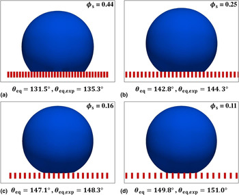
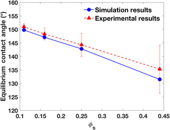
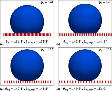
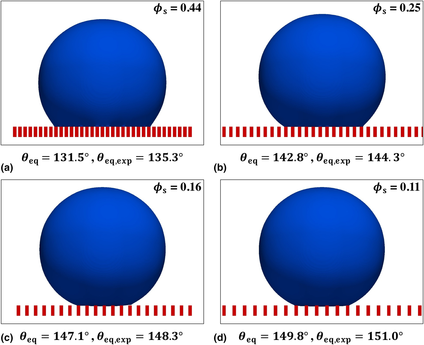
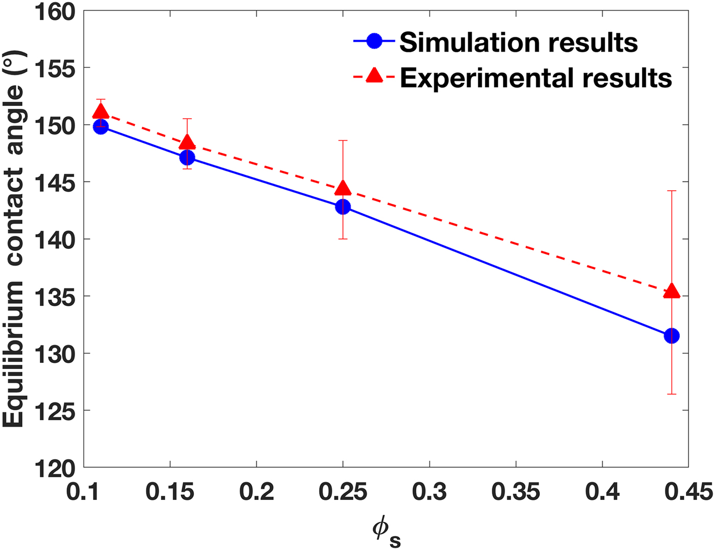
A 0.4 µL water droplet initially sits on the micro-patterned substrate. Its bottom is set with a small invasion distance of 12.5 µm below the pillar top-surface. As the simulation starts, the droplet bottom surface quickly recedes upward resulting in a decreased penetration depth. Within 5 ms, all four cases reach an equilibrium state, and yield the Cassie–Baxter state. Figure 3 presents the droplet contours at equilibrium conditions, and Fig. 4 compares the static apparent contact angles with the experimental data.[Reference Yao, Garvin, Alvarado, Jacobi, Jones and Marsh29] Results show good agreement between simulations and experiments. Screenshots of measuring the static contact angles using the KRUSS ADVANCE software are presented in Section 2 of the Supplementary materials. Note that the equilibrium contact angle is also referred to as the static contact angle (the two terms are used interchangeably).
The droplet contours of the equilibrium simulations with the measured apparent contact angles: (a) ϕ s = 0.44, (b) ϕ s = 0.25, (c) ϕ s = 0.16, and (d) ϕ s = 0.11.
The equilibrium contact angles compared with experimental data at different ϕ s.
Receding contact angles
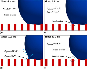
The receding (and advancing) contact angles are measured in the simulations by inserting a micropipette in the droplet as shown in Fig. 2(a). The volumetric outflow rate is 16 µL/s. Figure 5 shows the evolution of the droplet contour during the receding process in the case of ϕ s = 0.11. Although at t = 6.2 ms, the global contour is dominant, the liquid is pinned on the top-surface of the outermost pillar because of its hydrophilicity. At t = 9.8 ms, a local contour is developed near the outermost pillar. The global contact angle decreases slightly, and the local contact angle appears to be small (97.1°). At t = 12.6 ms, the local contour is increasingly noticeable, and the resulting local contact angle is only 41.7°. At t = 12.7 ms, the droplet recedes to the adjacent pillar, the global contour is recovered, and a small amount of water remains on the deserted pillar.
Evolution of the droplet contour (blue) in the receding process on the pillars (red) at ϕ s = 0.11: (a) at t = 6.2 ms, the global contour is dominant, (b) at t = 9.8 ms, a local contour is developed near the outermost pillar, (c) at t = 12.6 ms, the local contour becomes outstanding, and (d) at t = 12.7 ms, the droplet recedes to the neighboring pillar; the global contour is recovered; and a small amount of water remains on the previously outermost pillar.

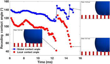
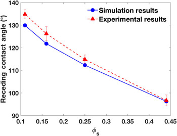
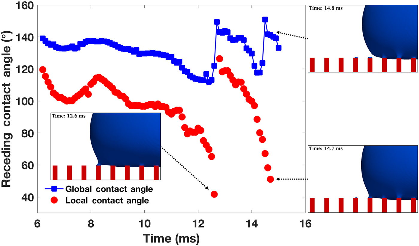
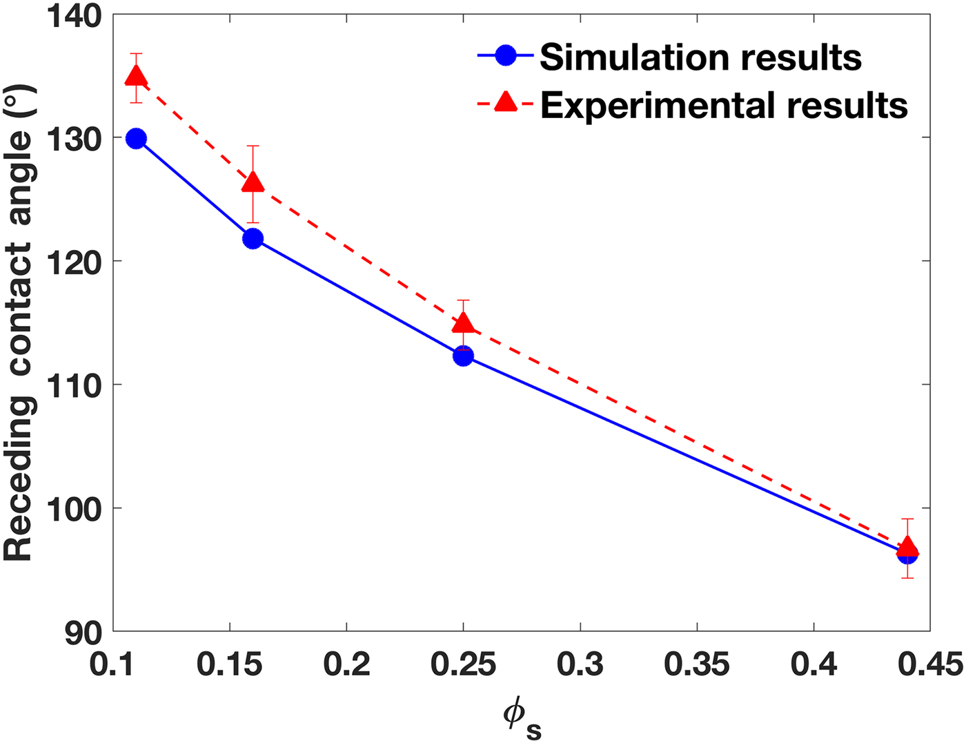
Figure 6 quantitatively depicts the evolution of receding contact angles in the time range of 6 < t < 15 ms. There are two jumps in both the global and local contact angles, at t = 12.6 ms, and t = 14.7 ms, each of which occurs when the contact line recedes from an outermost pillar to an adjacent one. In 6 < t < 12.6 ms, the first receding period occurs, and the rate of change of the contact angles is small, while, from 12.6 < t < 14.7 ms, a steady receding period is observed, and the rate of change is large. In both periods, the minimum local contact angle corresponds to the detaching moment, and afterward, it increases to about 130°. The minimum global contact angle is also observed at the same moment, but it quickly increases to about 150° after detaching. Both contact angles decrease as the contact line moves toward the adjacent pillar. Once the next pillar is reached, the contact angle sharply increases. The global contact angle is determined to be the receding contact angle. In this case, a medium value of 129.9° at t = 9.8 ms is reported as the receding contact angle, because it appears in the flat section of the global contact angle curve in Fig. 6. The same contact angle measurement procedure is performed for all the receding and advancing cases at different ϕ s. Figure 7 presents the receding contact angles at different ϕ s compared with experimental data. A good agreement has been observed. Videos of the receding simulations are provided as Movies S1–S4, and their snapshots are listed in Section 3 of the Supplementary materials.
Evolution of the receding contact angles at ϕ s = 0.11 for 6 <t <15 ms (global contact angles are marked using blue squares, and local contact angles using red circles).
The receding contact angles at different ϕ s compared with experimental results.
Advancing contact angles
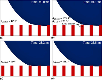
Similar to the receding cases, the advancing contact angles are measured using an inflow rate of 16 µL/s at the micropipette boundary. Figure 8 shows the evolution of the advancing process (20 ≤ t ≤ 21.8 ms) in the case of ϕ s = 0.11. A local contour develops near the outer, adjacent pillar next to the outermost pillar covered by the droplet. As a result, a local contact angle appears that differs from the global contact angle. The maximum local contact angle approaches 180°, however, it only lasts for an extremely short time (Δt < 0.1 ms), which is difficult to measure in experiments. In the advancing process, the hydrophilicity of the pillar top-surface plays an important role in attracting the liquid. After the contact line advances onto the adjacent pillar, the local contour disappears, and the global contact angle recovers a value similar to the former one.
The evolution of the droplet contour in an advancing process at ϕ s = 0.11: (a) t = 20.0 ms, (b) t = 21.1 ms, (c) t = 21.2 ms, and (d) t = 21.8 ms.
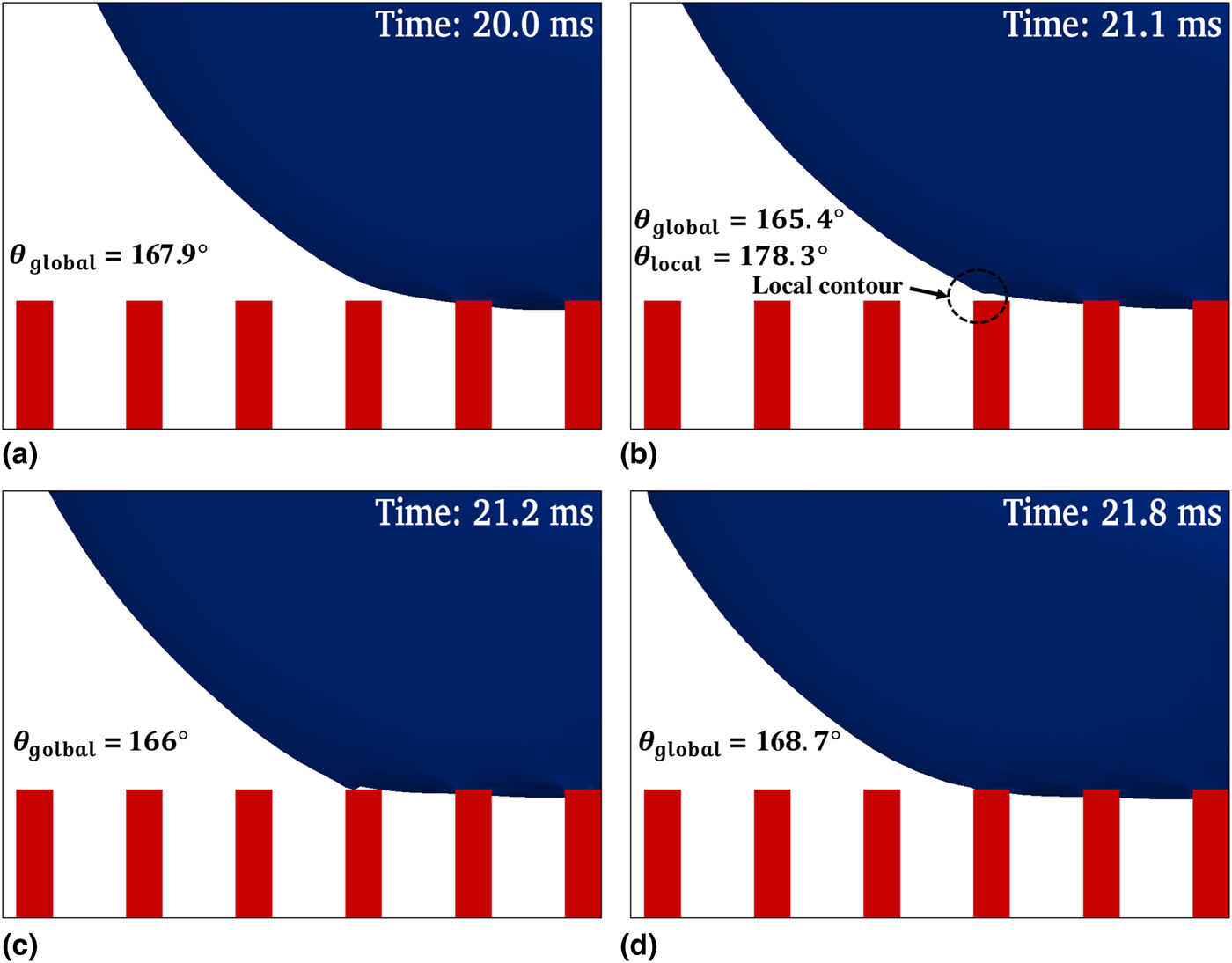
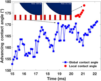
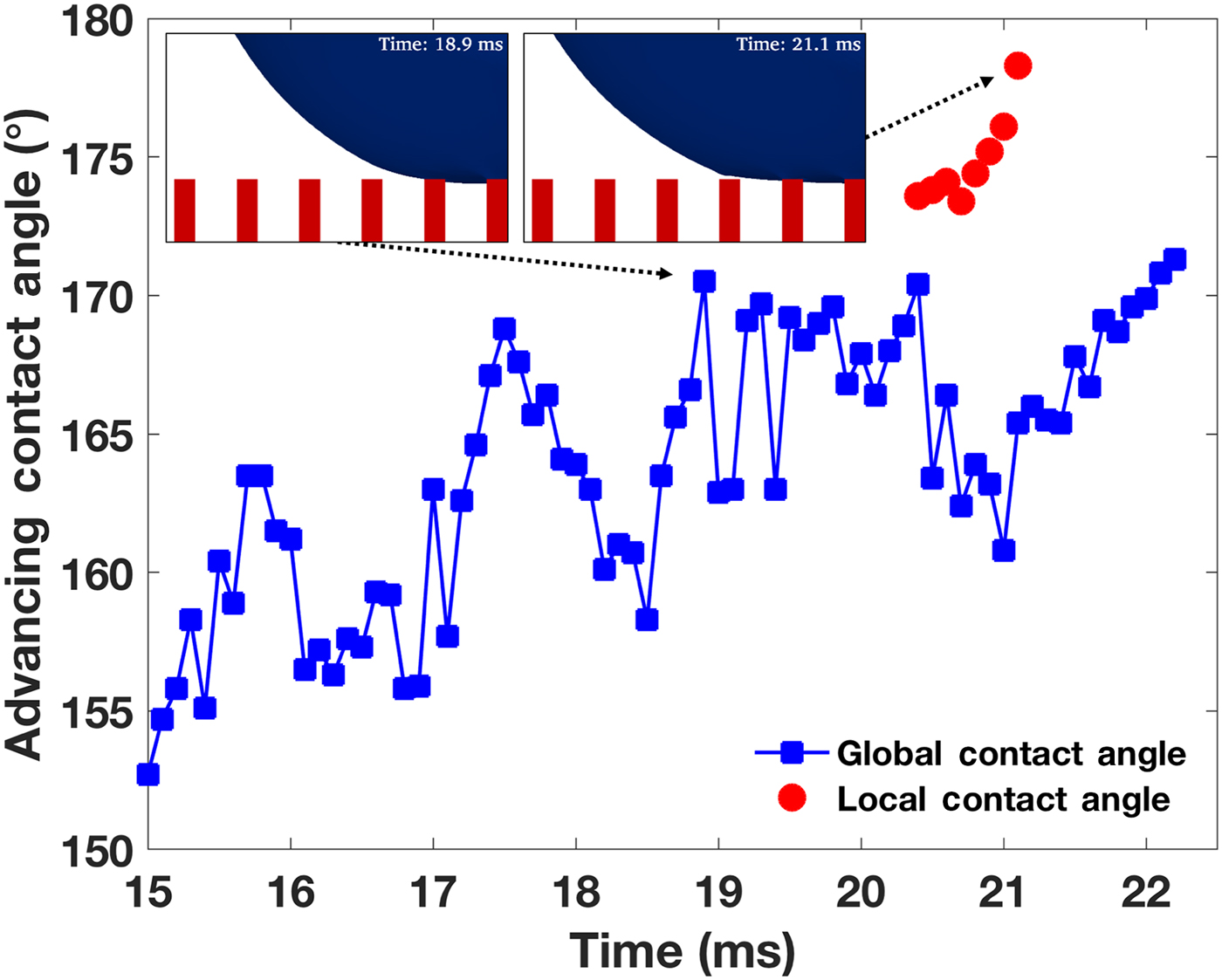
Figure 9 presents the evolution of the local and global advancing contact angles during 15 ≤ t ≤ 22 ms at ϕ s = 0.11. As the contact line advances, large fluctuations are observed in the global contact angle. Before the contact line approaches the adjacent pillar at t = 20.4 ms, fluctuation in the contact angle is caused by the fluid injection from the pipette. The droplet contour is disturbed by the inflow. After t = 20.4 ms, the contact line is strongly attracted by the hydrophilic top-surface of the adjacent pillar, and thus, induces contact angle fluctuations. As explained in the receding cases, the flat section (18.9 ≤ t ≤ 20.4 ms) of the global contact angle curve is reported as the advancing contact angle measured in this simulation. Videos of the advancing simulations are provided as Movies S5–S8, and their snapshots are listed in Section 4 of the Supplementary materials.
The evolution of the advancing contact angles at ϕ s = 0.11.
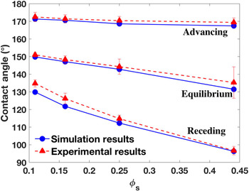
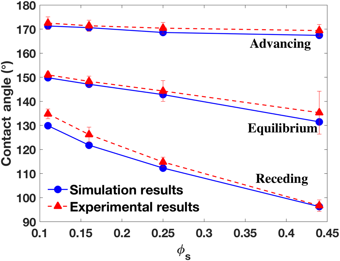
The equilibrium, receding and advancing contact angles are presented together with the experimental data of Ref. Reference Yao, Garvin, Alvarado, Jacobi, Jones and Marsh29 in Fig. 10. A good agreement has been achieved for all cases without fitting parameters, although small deviations exist for receding angles at small ϕ s. In addition, we note that the thin hydrophobic edge present on the pillar top-surface in the experiments, whose width is only 0.07 µm [see Fig. 1(c) and Table I in Ref. Reference Yao, Garvin, Alvarado, Jacobi, Jones and Marsh29], is extremely difficult to model in simulations because of the large scale difference.
The equilibrium, receding and advancing contact angles at different ϕ s compared with experimental results.
Droplet invasion and sagging
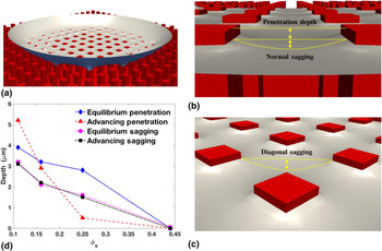
The invasion and sagging of the droplet into the pillar valleys are interesting, and will likely affect the surface energies; however, they are difficult to measure experimentally. Simulation studies exhibit advantages in predicting invasion and sagging. Figure 11 shows the penetration and sagging of the droplet bottom on the patterned substrate. Because of the hydrophobicity of the pillar top-surface, penetrations of a few micrometers have been observed in the equilibrium state for substrates, whose pillar spacings are large (ϕ s are 0.11, 0.16, 0.25), while zero penetration is observed for the substrate with the smallest pillar spacing (ϕ s = 0.44). As shown in Fig. 11(d), the penetration decreases with ϕ s, indicating that the required energy to invade the pillar valleys increases with ϕ s. In the advancing mode, the penetration at ϕ s = 0.11 is larger than that of the equilibrium state, because the inflow from the micropipette pushes the droplet surface toward the pillar bottom. However, at ϕ s = 0.16 and 0.25, the advancing penetration becomes lower than the equilibrium value. This is because (1) at higher ϕ s, the required energy to invade the pillar valleys increases, and (2) the advancing flow pushes the droplet interface in the lateral direction, and consequently, lifts the droplet bottom.
Penetration and sagging: (a) a cut view of the droplet bottom sitting on the patterned surface with ϕ s = 0.11, (b) the penetration depth and normal sagging, (c) the diagonal sagging marked for the same case, and (d) the penetration and diagonal-sagging depths at different ϕ s for the equilibrium and advancing modes.
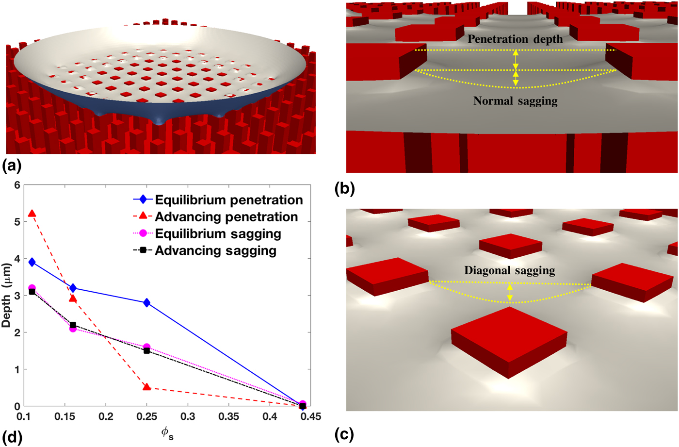
As shown in Figs. 11(b) and 11(c), normal sagging occurs between two adjacent pillars, while diagonal sagging occurs in the middle of four pillars. Obviously, the depth of diagonal sagging is larger than that of normal sagging. Figure 11(d) presents the diagonal sagging at different ϕ s for both the static and advancing modes. Because each pillar spacing is small (ranging from 12.5 to 50 µm), fluid flows cannot affect the liquid sagging. As a result, the advancing sagging depths are almost the same as the static values. More details for penetration and sagging are presented in Section 5 of the Supplementary materials.
Fluid flow and spurious velocity
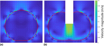
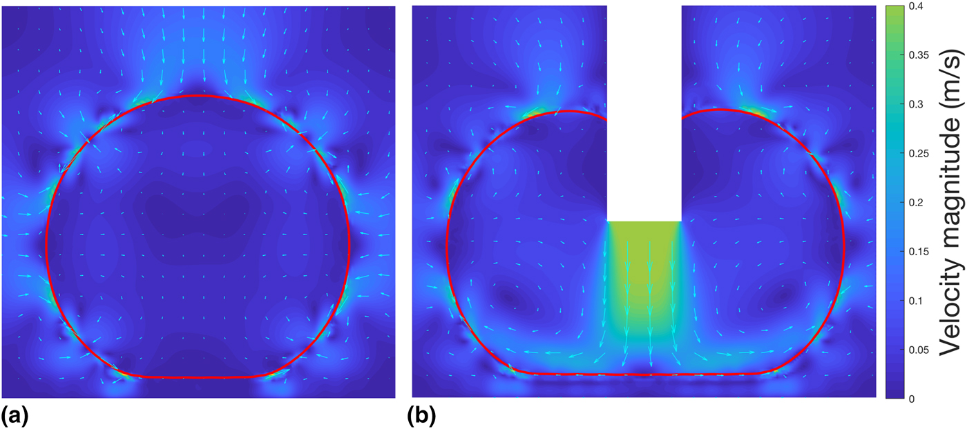
The VOF method used in this paper smears the liquid–gas interface, and induces spurious fluid flows near that interface, which raises the question, “Will the artificial flows affect the contact line dynamics, and so alter the apparent contact angles predicted on patterned substrates?” Figure 12 shows that the answer is no. At equilibrium [Fig. 12(a)], the spurious velocity is outstanding, while the bulk liquid remains stationary. The spurious velocity does not change the droplet contour, nor does it change the apparent contact angle. In the advancing mode [Fig. 12(b)], the spurious velocity is weaker than the inflow. It does not affect either the recirculation flows inside the droplet, or the apparent contact angle.
The magnitude (color) and vector (quivers) of the flow velocity on the central plane in (a) the equilibrium state, and (b) the advancing mode, both of which are at ϕ s = 0.11. The red line marks the droplet contour. While the pillars are not explicitly shown, their shadows can be seen in the flow field in (b). The empty rectangle in (b) is the micropipette.
Concluding remarks
In this paper, we developed a novel, constitutional contact line dynamics model based on the N–S equations capable of capturing the contact line motions of liquid interacting with a solid surface. Using our new method, a realistic continuum modeling has been achieved, and a series of 3-D simulations have been performed. These simulations allowed us to study a water droplet interacting with micrometer-sized pillared surfaces. Our model has been validated through comparing simulation results with the experimental results for four pillar spacings (12.5, 25, 37.5, and 50 µm), and three interacting modes (static, receding, and advancing). To the best of our knowledge, this is the first numerical study to report 3-D realistic, continuum simulations of static and dynamic contact angles. Our simulations captured the Cassie–Baxter state and reported apparent contact angles close to the experimental measurements at four pillar conditions and at three interacting modes. Good agreement on the static and dynamic contact angles and their trends indicates that our model captures the physical contact line dynamics.
Moreover, our simulations enable the detailed study of droplet–surface interactions, which are difficult to observe in experiments. The local and global contact angles have been captured in the receding and advancing cases when the contact line recedes or advances from one pillar to an adjacent one. This process is extremely brief (<0.1 ms). Our simulations also captured a small amount of residual water on a pillar from which the contact line had receded. The penetration and sagging of liquid into the pillar valleys have been reported. The high hydrophilicity of the pillar top-surface caused small penetrations of a few micrometers to be observed for large pillar spacings. However, further penetration was prevented by the high surface energy described in Section “Droplet invasion and sagging”, even if an initial penetration of 12.5 µm was set. The advancing mode is found to increase penetration at the largest pillar spacing and reduce it at the medium spacings. Zero penetration has been found for all cases with the smallest pillar spacings; this shows that the surface energy increases with ϕ s (i.e., decreasing with the pillar spacing). The sagging depth in the advancing mode is found to be the same as in the equilibrium state; this shows that the flow condition does not affect sagging for such a small scale present in pillar valleys.
The interface smearing technique is used in this modeling work, which induces spurious flows around the fluid–fluid interface. A natural question arises concerning the impact of artificial flows on the modeling of contact angles. Fortunately, our results showed that the spurious flows do not, in all cases, affect the overall droplet shape, the contact line dynamics, or the contact angles.
Future studies are planned to investigate the evolution of surface energy under different pillar conditions and droplet initial conditions.
Supplementary material
The supplementary material for this article can be found at https://doi.org/10.1557/mrc.2018.215.
Acknowledgment
The authors acknowledge the 2018 Research Enhancement Grant (REG) Award at LU for supporting this research. We acknowledge the Texas Advanced Computing Center (TACC) at UT Austin for funding computational hours (Grant #G-819854). We acknowledge the Center for Advances in Port Management at LU for funding our HPC cluster, and we thank the Center for Innovation, Commercialization and Entrepreneurship (CICE) at LU for supporting this research. We greatly appreciate Dr. Srinivas Palanki, Dr. Hsing-Wei Chu, Mr. Paul Latiolais, and Mr. Erik Stromberg for discussions and encouragement. We thank the IT Infrastructure Department at LU for hosting our HPC cluster, and especially thank Mr. Chad Smith for helping us on HPC maintenance.