1 Introduction
Recent times have seen a resurgence of interest in ship waves, the phenomenon whose theory was pioneered by Lord Kelvin well over a century ago (Thomson Reference Thomson1887). A topic of particular interest recently has been the angle formed by a ship’s waves. Famously, in deep waters the gravity-driven waves behind a ship were shown by Kelvin to lie within a sector of half-angle
 ${\it\Phi}_{\mathit{K}}=19^{\circ }28^{\prime }$
, regardless of the ship’s size, shape and velocity. Rabaud & Moisy (Reference Rabaud and Moisy2013) remarked, however, that images of ship wakes indicate the wake angle narrowing with increasing Froude number
 $Fr=V/\sqrt{gb}$
,
 $V$
being the ship’s velocity and
 $b$
its size. The issue was soon resolved by Darmon, Benzaquen & Raphaël (Reference Darmon, Benzaquen and Raphaël2014) and Noblesse et al. (Reference Noblesse, He, Zhu, Hong, Zhang, Zhu and Yang2014) who demonstrated that while Kelvin’s result remains true, the angle at which the waves’ amplitude is greatest is smaller than Kelvin’s angle, and decreases with increasing
 $Fr$
, making the wake appear narrower. The phenomenon was in fact observed and analysed already several decades ago (Munk, Scully-Power & Zachariasen Reference Munk, Scully-Power and Zachariasen1987; Brown et al.
Reference Brown, Buchsbaum, Hall, Penhune, Schmitt, Watson and Wyatt1989; Reed & Milgram Reference Reed and Milgram2002), and a number of authors have further elucidated this question recently (e.g. Benzaquen, Darmon & Raphaël Reference Benzaquen, Darmon and Raphaël2014; Moisy & Rabaud Reference Moisy and Rabaud2014; Pethiyagoda, McCue & Moroney Reference Pethiyagoda, McCue and Moroney2014, Reference Pethiyagoda, McCue and Moroney2015; He et al.
Reference He, Zhang, Zhu, Wu, Yang, Noblesse, Gu and Li2015; Zhu et al.
Reference Zhu, He, Zhang, Wu, Wan, Zhu and Noblesse2015). In particular it has been shown that interference effects between waves generated at the bow and the stern determine the scaling of the apparent angle with
 $Fr$
(Noblesse et al.
Reference Noblesse, He, Zhu, Hong, Zhang, Zhu and Yang2014; Zhang et al.
Reference Zhang, He, Zhu, Yang, Li, Zhu, Lin and Noblesse2015; Zhu et al.
Reference Zhu, He, Zhang, Wu, Wan, Zhu and Noblesse2015).
Although a large literature exists on waves on shear currents in two dimensions, or when the shear is horizontal (cf. e.g. Peregrine Reference Peregrine1976; Bühler Reference Bühler2009; Ellingsen & Brevik Reference Ellingsen and Brevik2014, and references therein), previous knowledge of waves on vertically sheared currents in three dimensions is very scarce and limited to a few scattered references (e.g. Craik Reference Craik1968; Johnson Reference Johnson1990; McHugh Reference McHugh1994). However, it was recently demonstrated that, when viscosity is neglected, a general solution to linear wave problems exists when a shear current with uniform vorticity is present, and the solution was used to solve the problems of ship waves (Ellingsen Reference Ellingsen2014b
), oscillating point source (Ellingsen & Tyvand Reference Ellingsen and Tyvand2016) and initial value problems (Ellingsen Reference Ellingsen2014a
; Li & Ellingsen Reference Li and Ellingsen2015). The presence of a shear current was found to influence the waves behind a ship profoundly. A ship travelling against the shear current (seen from a coordinate system where the unperturbed water surface is at rest) produces longer transverse wavelengths, and its wake is broader than Kelvin’s angle
 ${\it\Phi}_{\mathit{K}}$
, and vice versa for a ship travelling with the current. When the shear current makes an angle
 ${\it\beta}$
other than
 $0$
or
 ${\rm\pi}$
with the ship’s line of motion, the wake is found to be asymmetrical, its angular extent being greater than
 ${\it\Phi}_{\mathit{K}}$
on one side and smaller on the other. Moreover it was shown that, except at
 ${\it\beta}={\rm\pi}$
, there exists a critical velocity at which the Kelvin wake angle reaches a total angle of
 $180^{\circ }$
, beyond which the ship moves too fast for the transverse part of the ship waves to keep up, thus being unable to contribute to a stationary wake.
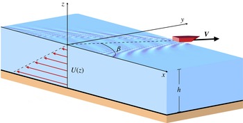
The geometry considered: a boat (modelled as a pressure disturbance) travelling at velocity
 $\boldsymbol{V}$
making an angle
 ${\it\beta}$
with an underlying shear current of uniform vorticity. The undisturbed surface is chosen to be at rest with respect to the coordinate system.

Waves carry momentum, so a moving wave source must feel a resistance force equal to the rate at which impulse is imparted to the waves which are created. This wave resistance force typically accounts for more than 30 % of the fuel consumption of large sea-going vessels (Faltinsen Reference Faltinsen2005). Knowing that the train of waves is affected by the presence of a subsurface shear current, it seems likely that also the wave resistance will be affected by the current, a notion which we confirm and quantify herein. In particular, when the ship’s line of motion is not parallel with the current the ship waves are asymmetrical, and the wave resistance also obtains a lateral component which, our calculations indicate, can amount to a significant percentage of the normal resistance force.
We present in the current paper a reasonably complete theory of linear ship waves in the presence of uniform vorticity when also the water is assumed to have a finite, constant depth
 $h$
. The geometry is shown in figure 1. While accounting for the finite depth is a straightforward extension of the formal derivation of general results, the physical implications are highly non-trivial, and introduce a subtle interplay between the effects of the shear current and the sea bed upon the surface elevation. We begin by laying out the theory in its general form and pay particular attention to the separation into near field and far field by careful use of the Cauchy integral theorem. The resulting far-field expression for the surface elevation differs slightly from that obtained by an alternative procedure (the Sokhotsky–Plemelj formula) used repeatedly in the literature, and we explain why the latter procedure is in fact potentially treacherous when employed, as here, in the context of the radiation condition.
We thereupon discuss in detail the phenomenon of critical velocity, which can occur whenever the dispersion relation makes the phase velocity bounded for all wavelengths in at least certain directions. Ship waves are termed supercritical when, for wave components in a finite sector of propagation directions, the ship’s velocity is greater than the maximum phase velocity measured along the direction of motion, in which case transverse waves will vanish from the ship wake completely. We derive explicit conditions for criticality and the critical velocity as a function of vorticity
 $S$
, depth and the angle
 ${\it\beta}$
.
Numerical evaluations of ship waves are thereafter carried out with particular emphasis on the transition between critical and non-critical waves; when the water depth is finite, increasing the shear can result in a transition both from subcritical to supercritical (as reported by Ellingsen Reference Ellingsen2014b ), or in certain cases, also from supercritical to subcritical. We finally calculate the wave resistance on the model ‘ship’, both the standard resistance force to the forward motion and the lateral force resulting from asymmetric wave making. While a realistic wave resistance calculation for a real vessel must take account of the actual hull shape, which is beyond our present scope, the calculations show trends which are likely to hold in general. Firstly, that wave resistance is increased when the ship motion has an upstream component (as seen from the system where the undisturbed surface is at rest), and decreased for downstream ship motion. Secondly, the Froude number at which the wave resistance is maximal is lowered for upstream and increased for downstream ship velocity.
2 Mathematical model and general solution
This section lays out the mathematical theory. The mathematical model and its general solution for wave pattern and wave resistance are derived in §§ 2.1 and 2.2 with (2.8), (2.12) and (2.14) as final results. A discussion of the dispersion relation ensues in § 2.3, whereupon far-field expressions are derived in § 2.4. It was seen as necessary to recount the careful extraction of the far-field waves in some detail herein, in order to highlight pitfalls and rectify errors associated with cavalier use of a related method used in recent literature. The final expression, (4.1), is found only after also taking on board lessons from § 3.
2.1 General solution
For fully three-dimensional flow in the presence of vorticity, potential theory is not an option, so to solve the flow problem we must turn to the Euler equations, describing inviscid flow. The flow is assumed to be incompressible. We write the full velocity and pressure field on the form
 $$\begin{eqnarray}\boldsymbol{v}=(U(z)+\hat{u} ,\hat{v},{\hat{w}});\quad P=-{\it\rho}gz+\hat{p};\quad U(z)=Sz.\end{eqnarray}$$
Here
 $U(z)$
is the basic shear current of constant vorticity
 $S\geqslant 0$
, and the hatted quantities are perturbations due to the waves. We shall assume all perturbations to be small, and work to linear order in these quantities. We have assumed the surface of the water to be at rest with respect to the coordinate system in order that results can be immediately compared to previous work: this is easily generalised by an overall Galilean coordinate transformation.
The wave source (‘ship’) is modelled as a superimposed localised pressure
 $\hat{p}_{ext}$
of constant shape and strength, travelling with velocity
 $\boldsymbol{V}$
which makes an angle
 ${\it\beta}$
with the
 $x$
axis, and hence the shear flow. The situation is sketched in figure 1. We consider only stationary solutions as seen from the boat, hence all physical quantities will depend on surface position
 $\boldsymbol{x}=(x,y)$
and time
 $t$
only through the combination
 ${\bf\xi}=\boldsymbol{x}-\boldsymbol{V}t$
. Such a stationary wake may be interpreted as a continuous series of ring waves emitted by the travelling source, and all our results might instead be derived based on such a formalism (Li & Ellingsen Reference Li and Ellingsen2016).
The flow is a solution to the Euler equation
 $$\begin{eqnarray}\partial _{t}\boldsymbol{v}+(\boldsymbol{v}\boldsymbol{\cdot }\boldsymbol{{\rm\nabla}})\boldsymbol{v}=-\boldsymbol{{\rm\nabla}}(P/{\it\rho}+gz)\end{eqnarray}$$
which we linearize with respect to perturbations. We use a Fourier decomposition of perturbation quantities into plane waves according to
 $$\begin{eqnarray}[\hat{u} ,\hat{v},{\hat{w}},\hat{p}]({\bf\xi},z)=\int \frac{\text{d}^{2}k}{(2{\rm\pi})^{2}}[u,v,w,p](\boldsymbol{k},z)\text{e}^{\text{i}\boldsymbol{k}\boldsymbol{\cdot }{\bf\xi}}.\end{eqnarray}$$
Following Ellingsen (Reference Ellingsen2014b
), we can eliminate
 $u,v$
and
 $p$
to find a simple Rayleigh equation (the inviscid form of the Orr–Sommerfeldt equation) for
 $w$
alone,
 $w^{\prime \prime }=k^{2}w.$
Solving this subject to the boundary condition that
 $w(\boldsymbol{k},-h)=0$
(no vertical velocity at the bottom), we find the solution to the full flow field as follows
 $$\begin{eqnarray}\displaystyle & \displaystyle u(\boldsymbol{k},z)=\text{i}A(\boldsymbol{k})\left[k_{x}\cosh k(z+h)+\frac{Sk_{y}^{2}\sinh k(z+h)}{k(k_{x}U-\boldsymbol{k}\boldsymbol{\cdot }\boldsymbol{V})}\right], & \displaystyle\end{eqnarray}$$
 $$\begin{eqnarray}\displaystyle & \displaystyle v(\boldsymbol{k},z)=\text{i}A(\boldsymbol{k})\left[k_{y}\cosh k(z+h)-\frac{Sk_{x}k_{y}\sinh k(z+h)}{k(k_{x}U-\boldsymbol{k}\boldsymbol{\cdot }\boldsymbol{V})}\right], & \displaystyle\end{eqnarray}$$
 $$\begin{eqnarray}\displaystyle & \displaystyle w(\boldsymbol{k},z)=kA(\boldsymbol{k})\sinh k(z+h), & \displaystyle\end{eqnarray}$$
 $$\begin{eqnarray}\displaystyle & \displaystyle p(\boldsymbol{k},z)=-\text{i}A(\boldsymbol{k})\left[(k_{x}U-\boldsymbol{k}\boldsymbol{\cdot }\boldsymbol{V})\cosh k(z+h)-\frac{Sk_{x}}{k}\sinh k(z+h)\right]. & \displaystyle\end{eqnarray}$$
 $A(\boldsymbol{k})$
is an unknown coefficient. These solutions are the ship wave equivalents of the general solutions reported by Ellingsen (Reference Ellingsen2014a
). Note that the motion introduced by this wave solution is itself rotational since it shifts and twists the vortex lines of the background flow, unlike any wave motion described by potential theory (Ellingsen Reference Ellingsen2016).
Let the surface elevation (relative to its equilibrium state) be
 ${\it\zeta}({\bf\xi})$
and the external pressure be
 $\hat{p}_{ext}({\bf\xi})$
, and let their Fourier transforms in the manner of (2.3), be
 $B(\boldsymbol{k})$
and
 $p_{ext}(\boldsymbol{k})$
, respectively. We can now write down the linearized kinematic boundary condition (stating that a particle on the surface stays on the surface)
 $$\begin{eqnarray}kA(\boldsymbol{k})\sinh kh=-\text{i}(\boldsymbol{k}\boldsymbol{\cdot }\boldsymbol{V})B(\boldsymbol{k})\end{eqnarray}$$
(note that
 $U(0)=0$
by choice), and dynamic boundary condition (stating that normal stress, as given by the pressure through Euler equation, is continuous at the surface),
 $$\begin{eqnarray}\text{i}A(\boldsymbol{k})\left[\boldsymbol{k}\boldsymbol{\cdot }\boldsymbol{V}\cosh kh+\frac{Sk_{x}}{k}\sinh kh\right]-gB(\boldsymbol{k})=p_{ext}(\boldsymbol{k})/{\it\rho}.\end{eqnarray}$$
Eliminating
 $A(\boldsymbol{k})$
, we find
 $B(\boldsymbol{k})$
which we integrate over the
 $\boldsymbol{k}$
plane to find
 ${\it\zeta}$
. One now encounters the same difficulty always encountered when considering waves in quasi-stationary or quasi-periodic wave systems, namely that the integral is indeterminate due to poles on the axes of integration. The criterion that our system, while being a stationary description, still knows the difference between past and future, must be imposed through a radiation condition. We use the procedure employed, e.g. by Lighthill (Reference Lighthill1978, § 3.9), presuming that the external pressure has been turned on very slowly since
 $t=-\infty$
 $$\begin{eqnarray}\hat{p}_{ext}\rightarrow p_{ext}\text{e}^{kV{\it\epsilon}t},\quad {\it\epsilon}=0^{+},\end{eqnarray}$$
where
 ${\it\epsilon}$
is defined to be dimensionless for convenience. The same slow temporal behaviour will affect all perturbation quantities, hence throughout our analysis this transition amounts to the replacement rule
 $\boldsymbol{k}\boldsymbol{\cdot }\boldsymbol{V}\rightarrow \boldsymbol{k}\boldsymbol{\cdot }\boldsymbol{V}+\text{i}kV{\it\epsilon}$
. The tiny addition to the ship’s ‘frequency’,
 $\boldsymbol{k}\boldsymbol{\cdot }\boldsymbol{V}$
, can be neglected except where it moves the pole slightly off the integration path, to complex values of
 $\boldsymbol{k}$
.
The resulting expression for the surface elevation is now well defined and reads
 $$\begin{eqnarray}\displaystyle & \displaystyle {\it\zeta}({\bf\xi})=-\frac{1}{{\it\rho}}\lim _{{\it\epsilon}\rightarrow 0^{+}}\int \frac{\text{d}^{2}k}{(2{\rm\pi})^{2}}\frac{kp_{ext}(\boldsymbol{k})\text{e}^{\text{i}\boldsymbol{k}\boldsymbol{\cdot }{\bf\xi}}}{gk-(\boldsymbol{k}\boldsymbol{\cdot }\boldsymbol{V})^{2}\coth kh-(\boldsymbol{k}\boldsymbol{\cdot }\boldsymbol{V})(Sk_{x}/k)-\text{i}{\it\epsilon}{\it\Phi}(\boldsymbol{k})}, & \displaystyle\end{eqnarray}$$
 $$\begin{eqnarray}\displaystyle & \displaystyle {\it\Phi}(\boldsymbol{k})=kV[2(\boldsymbol{k}\boldsymbol{\cdot }\boldsymbol{V})\coth kh+Sk_{x}/k]. & \displaystyle\end{eqnarray}$$
 $S=0$
. It is quite possible to use this expression directly for numerical purposes, keeping
 ${\it\epsilon}$
small but finite, as was done by Moisy & Rabaud (Reference Moisy and Rabaud2014). The effect of
 ${\it\epsilon}$
is to attenuate the waves slightly away from the boat. In § 2.4 we shall apply the Cauchy integral theorem as well as path of steepest descent techniques to obtain an expression for the far field only.
2.1.1 Gaussian pressure source
For definiteness, let us use the same Gaussian pressure source as used by Ellingsen (Reference Ellingsen2014a ,Reference Ellingsen b ) and also by Darmon et al. (Reference Darmon, Benzaquen and Raphaël2014):
 $$\begin{eqnarray}\hat{p}_{ext}({\bf\xi})=p_{0}\text{e}^{-({\rm\pi}{\it\xi}/b)^{2}};\quad p_{ext}(\boldsymbol{k})=\frac{b^{2}p_{0}}{{\rm\pi}}\text{e}^{-(kb/2{\rm\pi})^{2}}.\end{eqnarray}$$
As pointed out by He et al. (Reference He, Zhang, Zhu, Wu, Yang, Noblesse, Gu and Li2015), such a model of a ship will not give a completely realistic scaling of the ‘apparent wake angle’, the angle of maximum wave amplitude, for large Froude numbers, but this is not a point of focus in the present effort. It does, however, have the virtue of describing the size of the ‘ship’ by a single parameter
 $b$
, which in the presence of both shear and finite depth is seen as a great advantage for maintaining a manageable parameter space.
It is well known, and recently shown explicitly for a model like ours with an anisotropic Gaussian external pressure ‘ship’ model (Benzaquen et al.
Reference Benzaquen, Darmon and Raphaël2014), that the wave resistance depends on the shape of the ‘ship’. Thus our wave resistance calculations in the following must be understood as a demonstration of the theory, while quantitatively accurate wave resistance calculation requires using a source
 $\hat{p}_{ext}$
in (2.12) which approximates a particular hull shape. Such calculation is beyond the scope of the present effort. Note, however, that our formalism facilitates the use of more realistic models should quantitative results be needed in specific cases.
2.2 Wave resistance
The theory for wave resistance on a travelling pressure disturbance was laid out long ago in a series of papers by Havelock (Reference Havelock1917, Reference Havelock1919, Reference Havelock1922). This and other analytical models, as well as experimental results available at the time, were famously reviewed by Wehausen (Reference Wehausen1973). The effect of elongation of an ellipsoidal Gaussian pressure distribution was recently investigated by Benzaquen et al. (Reference Benzaquen, Darmon and Raphaël2014). The effect of shear upon wave resistance has never been considered before to our knowledge.
Havelock’s idea for calculation of wave resistance was to identify it as the horizontal component of the applied pressure force acting on the surface, in the direction of ship motion whereby the wave resistance may be found by an integral over the whole water surface:
 $$\begin{eqnarray}R=\int \,\text{d}^{2}{\it\xi}\,\hat{p}_{ext}({\bf\xi})(V^{-1}\boldsymbol{V}\boldsymbol{\cdot }\boldsymbol{{\rm\nabla}}_{{\it\xi}}){\it\zeta}({\bf\xi}),\end{eqnarray}$$
where
 $\boldsymbol{{\rm\nabla}}_{{\it\xi}}=(\partial /\partial {\it\xi}_{x},\partial /\partial {\it\xi}_{y})$
. Inserting (2.8), we recognise the complex conjugate of
 $p_{ext}$
and find
 $$\begin{eqnarray}R=-\frac{\text{i}}{{\it\rho}V}\lim _{{\it\epsilon}\rightarrow 0^{+}}\int \frac{\text{d}^{2}k}{(2{\rm\pi})^{2}}\frac{k(\boldsymbol{k}\boldsymbol{\cdot }\boldsymbol{V})|p_{ext}(\boldsymbol{k})|^{2}}{gk-(\boldsymbol{k}\boldsymbol{\cdot }\boldsymbol{V})^{2}\coth kh-(\boldsymbol{k}\boldsymbol{\cdot }\boldsymbol{V})(Sk_{x}/k)-\text{i}{\it\epsilon}{\it\Phi}(\boldsymbol{k})}.\end{eqnarray}$$
The limiting expression in deep water is again given by letting
 $\coth kh\rightarrow 1$
.
As shown by Ellingsen (Reference Ellingsen2014b
) the presence of a shear current beneath the boat will result in an asymmetric wake when the angle
 ${\it\beta}$
is not
 $0$
or
 ${\rm\pi}$
. This, in turn, will give a lateral force on the wave source, normal to the direction of motion. In a slight misuse of terminology we term it the ‘lateral wave resistance’
 $R_{\bot }$
, and it is found in analogous fashion
 $$\begin{eqnarray}R_{\bot }=\int \text{d}^{2}{\it\xi}\hat{p}_{ext}({\bf\xi})[V^{-1}(\mathbf{e}_{z}\times \boldsymbol{V})\boldsymbol{\cdot }\boldsymbol{{\rm\nabla}}_{{\it\xi}}]{\it\zeta}({\bf\xi}).\end{eqnarray}$$
A positive value of
 $R_{\bot }$
means a lateral force directed towards the right (starboard) with respect to the ship’s direction of motion. As for
 $R$
we find
 $$\begin{eqnarray}R_{\bot }=-\frac{\text{i}}{{\it\rho}V}\lim _{{\it\epsilon}\rightarrow 0^{+}}\int \frac{\text{d}^{2}k}{(2{\rm\pi})^{2}}\frac{k[(\mathbf{e}_{z}\times \boldsymbol{V})\boldsymbol{\cdot }\boldsymbol{k}]|p_{ext}(\boldsymbol{k})|^{2}}{gk-(\boldsymbol{k}\boldsymbol{\cdot }\boldsymbol{V})^{2}\coth kh-(\boldsymbol{k}\boldsymbol{\cdot }\boldsymbol{V})(Sk_{x}/k)-\text{i}{\it\epsilon}{\it\Phi}(\boldsymbol{k})}.\end{eqnarray}$$
2.3 Dispersion relation
Much of the physics of any wave problem may be discerned from analysis of the dispersion relation. As discussed in Ellingsen (Reference Ellingsen2014b
) (and numerous previous expositions without shear current present), the pole in the integrand of (2.8) – that is, the zero of the denominator – corresponds to values of
 $\boldsymbol{k}$
which simultaneously satisfy the dispersion relation and the condition of stationariness,
 $$\begin{eqnarray}\boldsymbol{k}\boldsymbol{\cdot }\boldsymbol{V}=kc(\boldsymbol{k})\end{eqnarray}$$
ensuring wave crests which look stationary as seen from the moving source.
 $c(\boldsymbol{k})$
is the phase velocity of a plane wave with wave vector
 $\boldsymbol{k}$
.
Letting the denominator of (2.8) (say) equal zero and solving with respect to
 $\boldsymbol{k}\boldsymbol{\cdot }\boldsymbol{V}$
immediately gives two solutions for the phase velocity,
 $$\begin{eqnarray}\boldsymbol{k}\boldsymbol{\cdot }\boldsymbol{V}=kc_{\pm }(\boldsymbol{k})=\pm \sqrt{gk\tanh kh+\left(\textstyle \frac{1}{2}S\cos {\it\theta}\tanh kh\right)^{2}}-\textstyle \frac{1}{2}S\cos {\it\theta}\tanh kh,\end{eqnarray}$$
where
 $\boldsymbol{k}=(k\cos {\it\theta},k\sin {\it\theta})$
. As discussed by Ellingsen (Reference Ellingsen2014a
), to each wave vector
 $\boldsymbol{k}$
there are two associated phase velocities. One of these phase velocities is positive, the other negative, and given the sign of
 $\boldsymbol{k}\boldsymbol{\cdot }\boldsymbol{V}$
, the appropriate solution is chosen.
For later reference let us denote the angle between
 $\boldsymbol{k}$
and
 $\boldsymbol{V}$
as
 ${\it\gamma}={\it\theta}-{\it\beta}$
, so that
 $$\begin{eqnarray}\boldsymbol{k}\boldsymbol{\cdot }\boldsymbol{V}=kV\cos {\it\gamma}.\end{eqnarray}$$
The constituents of the Fourier integral are plane waves with ‘frequency’
 $\boldsymbol{k}\boldsymbol{\cdot }\boldsymbol{V}$
which is negative when
 $|{\it\gamma}|>{\rm\pi}/2$
, and a wave of negative frequency and wave vector
 $\boldsymbol{k}$
has phase velocity in the direction of
 $-\boldsymbol{k}$
. Thus the integral in (2.8) (say) obtains two identical pole contributions, one from a wave of phase velocity
 $c_{+}$
whose wave vector has a forward component (
 $\boldsymbol{k}\boldsymbol{\cdot }\boldsymbol{V}>0$
) and one of phase velocity
 $c_{-}$
whose wave vector has a rearward component (
 $\boldsymbol{k}\boldsymbol{\cdot }\boldsymbol{V}<0$
). Both of these plane waves appear stationary as seen by the ship and give identical contributions.
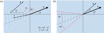
Definitions of the different angles used in the analysis.

While the coordinate system defined in figure 1 is easiest for the sake of the preceding derivations, for further analysis we shall want to use a polar system relative to the ship’s motion, in the manner of Ellingsen (Reference Ellingsen2014b ). We define
 $$\begin{eqnarray}{\it\phi}_{{\it\beta}}={\it\phi}-{\it\beta}.\end{eqnarray}$$
Using
 ${\it\gamma}$
and
 ${\it\phi}_{{\it\beta}}$
instead of
 ${\it\theta}$
and
 ${\it\phi}$
corresponds to rotating the coordinate system so that the boat moves along a new
 $x$
axis while the current, in general, does not. Definitions of the various angles used in the analysis are summarised in figure 2.
2.3.1 Length scales and limiting cases
Three length scales are involved in the model:
 $b$
(size of source),
 $h$
(depth) and a length associated with the shear,
 $l_{\mathit{S}}=g/S^{2}$
. Known limiting cases are obtained if one of the length scales is much greater than the smaller of the other two. When
 $l_{\mathit{S}}\gg \min (h,b)$
, the effect of shear becomes negligible, waves are the same for all
 ${\it\beta}$
, and the well-known expressions of Havelock (Reference Havelock1908) are regained. Likewise, when
 $h\gg \min (l_{\mathit{S}},b)$
, the deep water case considered by Ellingsen (Reference Ellingsen2014b
) is found, and the simplest case
 $b\ll h,l_{\mathit{S}}$
is detailed in Darmon et al. (Reference Darmon, Benzaquen and Raphaël2014), being the deep water case with no shear.
The most pertinent physical insights are obtained when these length scales are compared to typical wavelengths in different parts of the wake, as obtained from stationary phase arguments. Once typical values of
 $k$
and
 ${\it\theta}$
in some part of the wake (transverse or diverging waves), limiting cases can be analysed using the dispersion relation (2.16), which reveals that the effect of shear is weak provided
 ${\it\delta}\equiv \tanh kh/(kl_{\mathit{S}})\ll 1$
. In this case
 $$\begin{eqnarray}c_{\pm }(\boldsymbol{k})=c_{0}(k)\left(\pm 1-{\textstyle \frac{1}{2}}\sqrt{{\it\delta}}\cos {\it\theta}\pm {\textstyle \frac{1}{8}}{\it\delta}\cos ^{2}{\it\theta}+\cdots \!\right)\end{eqnarray}$$
with
 $c_{0}(k)=\sqrt{(g/k)\tanh kh}$
. We see that for the effect of shear upon a wave
 $\boldsymbol{k}$
to be small, it is sufficient that
 $|\sqrt{{\it\delta}}\cos {\it\theta}|\ll 1$
. There are thus two cases in which shear is rendered unimportant even though
 $kl_{\mathit{S}}$
is not large: if
 ${\it\theta}$
is close to
 $\pm {\rm\pi}/2$
(propagation normal to the shear current), or if
 $kh\ll 1$
(shallow water waves). The relative unimportance of shear for shallow water waves was shown for ring waves by Ellingsen (Reference Ellingsen2014a
).
2.4 Near-field and far-field contributions
We wish now to extract the far-field contribution to the ship waves. The analysis is carried out in a detailed and careful manner, thereby exposing weaknesses in a more cavalier method used in the recent literature, including Darmon et al. (Reference Darmon, Benzaquen and Raphaël2014) and Ellingsen (Reference Ellingsen2014b ). In order not to clutter the reading overly with mathematics, some calculations are found in appendices.
We will re-write the expression for the surface elevation (2.8) with a Gaussian disturbance in a different form which is suitable for further analysis. First, let us write the integral over
 $\boldsymbol{k}$
in polar form with dimensionless quantities,
 $$\begin{eqnarray}\displaystyle & \displaystyle {\it\zeta}(\boldsymbol{X})=\frac{bp_{0}}{4{\rm\pi}^{3}{\it\rho}V^{2}}\int _{-{\rm\pi}}^{{\rm\pi}}\frac{\text{d}{\it\gamma}}{\cos ^{2}{\it\gamma}}\lim _{{\it\epsilon}\rightarrow 0^{+}}I({\it\gamma}) & \displaystyle\end{eqnarray}$$
 $$\begin{eqnarray}\displaystyle & \displaystyle I({\it\gamma})=\int _{0}^{\infty }\text{d}KK\frac{\text{e}^{E(K,{\it\gamma})}\tanh KH}{{\it\Gamma}(K,{\it\gamma})+\text{i}{\it\epsilon}{\it\Psi}(K,{\it\gamma})}\equiv \int _{0}^{\infty }\text{d}Kf(K,{\it\gamma}) & \displaystyle\end{eqnarray}$$
 $$\begin{eqnarray}\boldsymbol{K}=b\boldsymbol{k},\quad \boldsymbol{X}={\bf\xi}/b,\quad H=h/b.\end{eqnarray}$$
and the functions (for frequent reference below)
 $$\begin{eqnarray}\displaystyle & \displaystyle E(K,{\it\gamma})=-K^{2}/4{\rm\pi}^{2}+\text{i}KX\cos ({\it\gamma}-{\it\phi}_{{\it\beta}}), & \displaystyle\end{eqnarray}$$
 $$\begin{eqnarray}\displaystyle & \displaystyle {\it\Gamma}(K,{\it\gamma})=K-\frac{f_{s}({\it\gamma})}{Fr^{2}\cos ^{2}{\it\gamma}}\tanh KH, & \displaystyle\end{eqnarray}$$
 $$\begin{eqnarray}\displaystyle & \displaystyle {\it\Psi}(K,{\it\gamma})=\frac{2K}{\cos {\it\gamma}}+\frac{Fr_{\mathit{s}}}{Fr^{2}}\frac{\cos ({\it\gamma}+{\it\beta})}{\cos ^{2}{\it\gamma}}\tanh KH, & \displaystyle\end{eqnarray}$$
 $$\begin{eqnarray}\displaystyle & \displaystyle f_{s}({\it\gamma})=1-Fr_{\mathit{s}}\cos {\it\gamma}\cos ({\it\gamma}+{\it\beta}). & \displaystyle\end{eqnarray}$$
Our system is described by four non-dimensional parameters:
 $Fr,Fr_{\mathit{s}},Fr_{h}$
and
 ${\it\beta}$
, where the three Froude numbers are
 $$\begin{eqnarray}Fr=\frac{V}{\sqrt{gb}};\quad Fr_{\mathit{s}}=\frac{VS}{g};\quad Fr_{h}=\frac{V}{\sqrt{gh}}.\end{eqnarray}$$
Here
 $Fr$
is based on the size of the source (the ship),
 $Fr_{\mathit{s}}$
is based on a ‘shear depth’
 $g/S^{2}$
which is half the depth at which the dynamic and hydrostatic pressure of the shear flow are equal, and
 $Fr_{h}$
is based on the finite water depth.
We will consider the integral
 $I({\it\gamma})$
by forming a closed contour in the complex
 $K$
plane. The contour is formed of the positive real
 $K$
axis (the original integration path) and closed either in the upper or lower plane, depending on the exponent function
 $E(K,{\it\gamma})$
so that the resulting path gives a finite and well defined integral. To wit we shall choose the path of steepest descent (cf. e.g. Bender & Orszag Reference Bender and Orszag1991, § 6.6),
 $$\begin{eqnarray}K_{s.d.}(K,{\it\gamma})=K+2{\rm\pi}^{2}\text{i}X\cos ({\it\gamma}-{\it\phi}_{{\it\beta}}).\end{eqnarray}$$
This path is parallel to the real
 $K$
axis and lies either above or below the latter depending on the sign of
 $\cos ({\it\gamma}-{\it\phi}_{{\it\beta}})$
. We connect it to the original path of integration while noticing that
 ${\it\Gamma}(K,{\it\gamma})$
has a series of zeros along the imaginary axis which we wish to avoid, and therefore choose the connection path (arbitrarily) at
 $45^{\circ }$
to the real axis. The path is closed at infinity where the integrand is exponentially zero. The closed path of integration,
 ${\it\Lambda}$
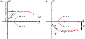
, is shown in figure 3.
Contours of integration: the original integration path along the positive real
 $K$
axis is closed with a steepest descent path and a connection path at an angle with both axes. The position of the pole is indicated, its position relative to the real
 $K$
axis depending on the sign of the function
 $F(K_{0},{\it\gamma})$
. (a)
 $\cos ({\it\gamma}-{\it\phi}_{{\it\beta}})>0$
, (b)
 $\cos ({\it\gamma}-{\it\phi}_{{\it\beta}})<0$
.

Now we define
 $K_{0}({\it\gamma})$
as the (real) value of
 $K$
for which
 ${\it\Gamma}(K,{\it\gamma})$
has a zero, i.e. it is implicitly defined by
 $$\begin{eqnarray}K_{0}-\frac{f_{s}({\it\gamma})}{Fr^{2}\cos ^{2}{\it\gamma}}\tanh K_{0}H=0.\end{eqnarray}$$
Only in the deep water limit
 $H\rightarrow \infty$
is the expression for
 $K_{0}$
explicit. For a given set of parameters, it is not certain that a positive solution of (2.25) exists. Note that the trivial solution
 $K_{0}=0$
is not a pole of the integrand since it is cancelled by a factor
 $K$
in the numerator. The existence or non-existence of a positive solution
 $K_{0}({\it\gamma})$
is related to the question of a critical velocity, and is discussed in § 3. There, an approximate, explicit solution for
 $K_{0}({\it\gamma})$
is also given.
Importantly, when
 $K_{0}$
is inserted for
 $K$
, the exponent function
 $E(K_{0},{\it\gamma})$
does not depend on the source size
 $b$
, i.e. on the Froude number
 $Fr$
. This is important because the pole at
 $K=K_{0}$
gives far-field waves (to be shown below), and the exponent function
 $E(K_{0},{\it\gamma})$
is what determines the width of the Kelvin wake. Hence, just as was for deep water (Ellingsen Reference Ellingsen2014b
) (and is well-known to be the case without shear), the source Froude number has no influence on the Kelvin angle, although it strongly affects the apparent wake angle at which the waves have the largest amplitude (see, e.g. Darmon et al.
Reference Darmon, Benzaquen and Raphaël2014; Noblesse et al.
Reference Noblesse, He, Zhu, Hong, Zhang, Zhu and Yang2014).
We now proceed to solve the contour integral
 $I({\it\gamma})$
. We show in § A.2 that the integrals
 $I_{s.d.}$
and
 $I_{conn.}$
make up the near field of the wake, i.e. a surface deformation following the source which falls off quickly as
 $X$
increases. The all-important far field of the wave pattern is given by the contribution from the pole, provided it is found inside the contour. This should be no surprise, since exactly this decomposition has been reported numerous times in the literature (e.g. Lighthill Reference Lighthill1978) for ship waves as well as other wave systems.
Evaluating the contribution from the pole (details may be found in § A.1) we obtain the following expression for the far field of the wave pattern
 $$\begin{eqnarray}\displaystyle {\it\zeta}_{\mathit{f.f.}} & = & \displaystyle -\frac{\text{i}p_{0}}{2{\rm\pi}^{2}{\it\rho}g}\int _{-{\rm\pi}}^{{\rm\pi}}\text{d}{\it\gamma}{\it\Theta}(K_{0}){\it\Theta}[-\!\cos ({\it\gamma}-{\it\phi}_{{\it\beta}})\cos {\it\gamma}]Sg\,[\cos {\it\gamma}]\nonumber\\ \displaystyle & & \displaystyle \times \,\frac{K_{0}\text{e}^{E(K_{0})}\tanh K_{0}H}{Fr^{2}\cos ^{2}{\it\gamma}-Hf_{s}({\it\gamma})\text{sech}^{2}K_{0}H}.\end{eqnarray}$$
Here
 ${\it\Theta}$
is the Heaviside step function.
Crucially, once the far field is identified as the contribution to
 $I({\it\gamma})$
from the pole, it implies that a wave of propagation direction
 ${\it\gamma}$
contributes to the far field in the real space direction
 ${\it\phi}$
if and only if the pole where
 ${\it\Gamma}+\text{i}{\it\epsilon}{\it\Psi}=0$
lies inside the contour
 ${\it\Lambda}$
. Much of the below analysis rests upon this insight, and we shall see that the two different ways in which the pole can fall outside the contour, corresponding to the two Heaviside functions in (2.26), each have their different physical interpretations.
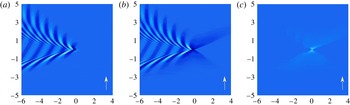
Illustration of wake waves calculated using the expressions for (a) the full expression in (2.8), (b) the far-field expression in (2.26), and (c) only the near field. In (a–c)
 $Fr=Fr_{\mathit{s}}=0.8$
,
 $Fr_{h}=0$
and
 ${\it\beta}={\rm\pi}/2$
. Arrows indicate direction of shear flow as defined in figure 1.

The separation into near field and far field are shown in figure 4. One may note that the far field as calculated with the Cauchy integral theorem gives a butterfly like surface deformation near the source, which is particularly visible with strong side-on shear such as shown in figure 4. The artefact is not a worry since the far-field expression is only accurate far from the source.
The requirement that the pole most lie inside the closed contour in order to contribute led to the Heaviside factor
 ${\it\Theta}[-\!\cos ({\it\gamma}-{\it\phi}_{{\it\beta}})\cos {\it\gamma}]$
in (2.26). A careful inspection of the angles involved reveals that this factor restricts the contribution to the far field to including only the partial waves whose direction of propagation has a positive component towards the ship. In other words, the waves in the far field always follow the ship and are not allowed to run ahead of it. This accords well with what one must expect, but we note that arguments based on the group velocity, say, would be complicated since in the presence of shear the phase and group velocities do not in general have the same direction.
The radiation condition used here automatically allows for the perhaps surprising result that with side-on shear near the critical velocity, waves can in fact be seen in front of the moving ship on one side (see § 4 and Ellingsen (Reference Ellingsen2014b )). This is not in violation of the radiation condition because these waves have been sufficiently refracted by the shear to still be able to follow the moving source according to the above definition.
Note finally that, beyond being a generalization, the far-field expression in (2.26) in fact differs slightly from those reported in Ellingsen (Reference Ellingsen2014b
), Darmon et al. (Reference Darmon, Benzaquen and Raphaël2014), Benzaquen et al. (Reference Benzaquen, Darmon and Raphaël2014). In these references the Sokhotsky–Plemelj formula was used to extract the far-field contribution from an expression similar, but not identical, to (2.8). We explain in appendix B why the use of this theorem is treacherous; it yields a far-field expression which but for a factor
 $2$
is identical to ours in the limit
 $X\rightarrow \infty$
behind the ship, but which contains a spurious wake also in front of the ship which is equal but of opposite sign. Clearly such a far field does not satisfy the radiation condition at positions within the spurious Kelvin wedge in front of the ship, the reason for which appendix B elucidates. When Sokhotsky–Plemelj is used, the spurious wake must be manually removed from the far-field expression, for instance by simply not plotting it. This is easy and clear cut in deep waters with no shear current, when the wave train is famously contained within a Kelvin wedge with half-angle
 $19^{\circ }28^{\prime }$
, but not so straightforward when the wake angle grows large or even extends beyond
 $90^{\circ }$
. Moreover, Ellingsen (Reference Ellingsen2014b
) and Darmon et al. (Reference Darmon, Benzaquen and Raphaël2014) perform integration over
 ${\it\gamma}$
only from
 $-{\rm\pi}/2$
to
 ${\rm\pi}/2$
, resulting in a further factor
 $2$
difference and a far-field expression which is an overall factor
 $4$
smaller than our (2.26). This does not affect any of the main conclusions in these references.
3 Critical velocity
In this section we discuss the phenomenon of critical velocity, and derive the criterion for criticality, (3.8), when both shear and finite depth are present.
The phenomenon of critical velocity is known previously both for ship waves in shallow water (Havelock Reference Havelock1908) and in shear current (Ellingsen Reference Ellingsen2014b
). In physical terms, when the ship’s speed exceeds a certain critical velocity, transverse-propagating waves (i.e. the part of the ship waves whose direction of propagation
 $\boldsymbol{k}$
is close to parallel with
 $\boldsymbol{V}$
, found directly behind the ship in a wedge including
 ${\it\phi}_{{\it\beta}}={\rm\pi}$
) are unable to keep up with the source and cannot contribute to a stationary wake as seen by the moving source. We will show that the criterion that
 $K_{0}({\it\gamma})$
must exist for waves contributing to the far field is exactly the criterion which ensures that transverse plane wave components are excluded at supercritical velocities.
Below we will derive the following explicit expression for the critical Froude number and velocity,
 $$\begin{eqnarray}Fr_{crit}=\frac{V_{\mathit{crit}}}{\sqrt{gb}}=\frac{\sqrt{Fr_{Sb}^{2}+1/H}-Fr_{Sb}\cos {\it\beta}}{1/H+Fr_{Sb}^{2}\sin ^{2}{\it\beta}},\end{eqnarray}$$
where the intrinsic Froude number (based on the velocity
 $Sb$
and the source size
 $b$
) is
 $$\begin{eqnarray}Fr_{Sb}=\frac{Sb}{2\sqrt{gb}}=\frac{S}{2}\sqrt{\frac{b}{g}}.\end{eqnarray}$$
While it is true that the amplitude of the transverse waves in the wake decreases as the ship’s velocity (hence
 $Fr$
) increases, and they gradually vanish from sight (Darmon et al.
Reference Darmon, Benzaquen and Raphaël2014), the vanishing of transverse waves is not the only, or even the most, striking phenomenon associated with the critical velocity. As
 $V$
approaches the critical, the total Kelvin wake angle reaches
 ${\rm\pi}$
in a sharp peak at this velocity, as will be duly discussed in the following. The phenomenon cannot be observed in deep, still waters since it is caused by the fact that phase velocity is limited: In shallow waters, the phase velocity cannot exceed
 $\sqrt{gh}$
, and in a shear current
 $c(\boldsymbol{k})$
is limited above by
 $g/S\cos {\it\theta}$
when
 ${\it\theta}>0$
(propagation against the shear) as may be deduced from (2.16).
As argued, the value of the wavenumber which satisfies both the dispersion relation and the condition that the wave front appears stationary as seen from the boat is
 $K_{0}({\it\gamma})$
, solving (2.25). Only such a plane wave can contribute to the ship wave pattern in the far field. It is useful to write (2.25) in the form
 $$\begin{eqnarray}f({\it\varkappa})\equiv {\it\varkappa}-B({\it\gamma})\tanh {\it\varkappa}=0\end{eqnarray}$$
with
 ${\it\varkappa}=K_{0}H$
and
 $B({\it\gamma})=f_{s}({\it\gamma})/(Fr_{h}^{2}\cos ^{2}{\it\gamma})$
. For any real
 $B({\it\gamma})$
the function
 $f({\it\varkappa})$
is smooth, positive as
 ${\it\varkappa}\rightarrow \infty$
and is zero at
 ${\it\varkappa}=0$
, hence it follows that
 $f({\it\varkappa})$
has a zero at some positive
 ${\it\gamma}$
if and only if
 $f^{\prime }(0)<0$
, that is, if
 $B>1$
. Thus the criterion for a positive solution
 $K_{0}({\it\gamma})>0$
to exist for some value of
 ${\it\gamma}$
is that
 $B({\it\gamma})>1$
, which can be written
 $$\begin{eqnarray}1-Fr_{\mathit{s}}\cos {\it\gamma}\cos ({\it\gamma}+{\it\beta})-Fr_{h}^{2}\cos ^{2}{\it\gamma}>0.\end{eqnarray}$$
An approximate solution to (3.3) for
 ${\it\varkappa}$
as a function of
 ${\it\gamma}$
expressed as a functional of
 $B({\it\gamma})$
may be found by matching the asymptotic behaviours at
 $B\rightarrow \infty$
and
 $B\rightarrow 1$
,
 $$\begin{eqnarray}{\it\varkappa}_{\mathit{app}}=B({\it\gamma})-1+\sqrt{1-B({\it\gamma})^{-3}}.\end{eqnarray}$$
The approximation remains better than approximately
 $8$
% accurate for all
 $B>1$
, and is
 $1\,\%$
accurate or better for
 $B\gtrsim 2$
.
3.1 Condition of criticality
We will now derive and discuss the critical velocity in the present case in which both finite depth (parameterised though
 $Fr_{h}$
) and shear current (parameterised through
 $Fr_{\mathit{s}}$
) are present. Either of the two on its own will give rise to a finite critical velocity, and combining the two naturally yields a critical velocity which depends on both
 $Fr_{h}$
and
 $Fr_{\mathit{s}}$
, as well as the angle
 ${\it\beta}$
between ship motion and shear current.
We shall describe a situation given by parameter triplet
 $Fr_{h},Fr_{\mathit{s}},{\it\beta}$
as supercritical if a finite sector of
 ${\it\gamma}$
values exists wherein the criterion (3.4) is false. It is slightly easier mathematically to work with the rearranged condition, equivalent to (3.4),
 $$\begin{eqnarray}\frac{1-Fr_{\mathit{s}}\cos {\it\gamma}\cos ({\it\gamma}+{\it\beta})}{\cos ^{2}{\it\gamma}}>Fr_{h}^{2}\end{eqnarray}$$
(we presume
 $\cos {\it\gamma}\neq 0$
). The situation is supercritical if
 $$\begin{eqnarray}\min _{{\it\gamma}}\left\{\frac{1-Fr_{\mathit{s}}\cos {\it\gamma}\cos ({\it\gamma}+{\it\beta})}{\cos ^{2}{\it\gamma}}\right\}<Fr_{h}^{2},\end{eqnarray}$$
where the notation means the minimum of the left-hand side with respect to
 ${\it\gamma}$
is taken. The minimum is found at
 $\tan {\it\gamma}=-(Fr_{\mathit{s}}\sin {\it\beta})/2$
, which we reinsert and conclude that the situation is supercritical if
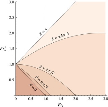
 $$\begin{eqnarray}Fr_{\mathit{s}}(\cos {\it\beta}+\textstyle \frac{1}{4}Fr_{\mathit{s}}\sin ^{2}{\it\beta})+Fr_{h}^{2}>1.\end{eqnarray}$$
The sub and supercritical regions of the
 $Fr_{\mathit{s}}$
–
 $Fr_{h}$
parameter plane are shown in figure 5 for some values of
 ${\it\beta}$
.
Critical lines as function of
 $Fr_{\mathit{s}}$
and
 $Fr_{h}$
for different values of
 ${\it\beta}$
. The shaded regions below the critical lines are subcritical.

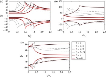
Kelvin angles for constant
 $Fr_{\mathit{s}}=0.5$
(a), constant
 $Fr_{h}^{2}=0.75$
(b) and constant
 $Fr_{h}^{2}=1.25$
(c). The case
 $Fr_{\mathit{s}}=0$
is also shown in (a) for comparison. See also figure 8.

Inserting the definitions of
 $Fr_{\mathit{s}}$
and
 $Fr_{h}$
, (3.8) can be solved with respect to
 $V$
to obtain the critical velocity given in (3.1). The known limits when
 $S=0$
(no shear current) when
 $V_{\mathit{crit}}=\sqrt{gh}$
(Havelock Reference Havelock1908), and as
 $h\rightarrow \infty$
when
 $V_{\mathit{crit}}=S/g\cos ^{2}({\it\beta}/2)$
(Ellingsen Reference Ellingsen2014b
), are regained. The latter limit may be seen easily if one notes that (3.8) can instead be written
 $$\begin{eqnarray}\frac{Fr_{h}^{2}}{1+Fr_{\mathit{s}}\sin ^{2}({\it\beta}/2)}+Fr_{\mathit{s}}\cos ^{2}({\it\beta}/2)>1.\end{eqnarray}$$
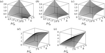
We plot
 $Fr_{crit}$
in figure 7.
 $Fr_{crit}$
as a function of
 $h$
and
 $Fr_{Sb}$
for different values of
 ${\it\beta}$
. (a)
 ${\it\beta}=0$
;(b)
 ${\it\beta}={\rm\pi}/4$
; (c)
 ${\it\beta}={\rm\pi}/2$
; (d)
 ${\it\beta}=3{\rm\pi}/4$
; (e)
 ${\it\beta}={\rm\pi}$
.

4 Wave patterns and Kelvin angles under different conditions
In this section we present numerical evaluation of wave patterns and Kelvin angles (total angular extent of the wake) in different parts of the parameter space spanned by parameters
 $Fr,Fr_{\mathit{s}},Fr_{h}$
and
 ${\it\beta}$
.
Combining what has been found so far, the far field of the surface elevation can be written
 $$\begin{eqnarray}\displaystyle {\it\zeta}_{\mathit{f.f.}} & = & \displaystyle \frac{p_{0}}{2{\rm\pi}^{2}{\it\rho}g}\int _{-{\rm\pi}}^{{\rm\pi}}\text{d}{\it\gamma}{\it\Theta}[1-Fr_{\mathit{s}}\cos {\it\gamma}\cos ({\it\gamma}+{\it\beta})-Fr_{h}^{2}\cos ^{2}{\it\gamma}]Sg\,[\cos {\it\gamma}]\nonumber\\ \displaystyle & & \displaystyle \times \,{\it\Theta}[-\!\cos ({\it\gamma}-{\it\phi}_{{\it\beta}})\cos {\it\gamma}]\frac{K_{0}\text{e}^{-(K_{0}/2{\rm\pi})^{2}}\sin [K_{0}X\cos ({\it\gamma}-{\it\phi}_{{\it\beta}})]\tanh K_{0}H}{Fr^{2}\cos ^{2}{\it\gamma}-Hf_{s}({\it\gamma})\text{sech}^{2}K_{0}H},\quad\end{eqnarray}$$
where we have now taken the real part. Significant contributions to the far field are only obtained for values of
 ${\it\phi}_{{\it\beta}}$
where the argument of the sine,
 $$\begin{eqnarray}f_{1}({\it\gamma})=K_{0}({\it\gamma})X\cos ({\it\gamma}-{\it\phi}_{{\it\beta}})\end{eqnarray}$$
has a stationary point for a value of
 ${\it\gamma}$
in the integration range, that is, where
 $\partial _{{\it\gamma}}f_{1}({\it\gamma})=0$
. The Kelvin angle as defined in Darmon et al. (Reference Darmon, Benzaquen and Raphaël2014) and Ellingsen (Reference Ellingsen2014b
) is the largest value of
 $|{\rm\pi}-{\it\phi}_{b}|$
for which a stationary point exists; in the presence of a shear current the Kelvin angle is in general different on either side of the wake.
Unlike the cases considered in these references, we do not now have an explicit expression for
 $K_{0}({\it\gamma})$
or its derivative, so the Kelvin angle must be found numerically by first calculating the value of
 ${\it\phi}_{{\it\beta},stat}({\it\gamma})$
at which a stationary point exists for a given value of
 ${\it\gamma}$
and then finding the extrema of
 ${\rm\pi}-{\it\phi}_{{\it\beta},stat}({\it\gamma})$
in the range of
 ${\it\gamma}$
(see also Ellingsen Reference Ellingsen2014b
, for details and illustration).
Kelvin angles for different values of
 $Fr_{\mathit{s}}$
and
 $Fr_{h}^{2}$
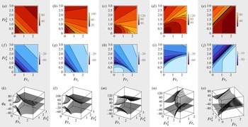
: left-hand Kelvin angle (a–e), right-hand Kelvin angle (f–j) for
 ${\it\beta}=0$
(a,f,k);
 ${\rm\pi}/4$
(b,g,l);
 ${\rm\pi}/2$
(c,h,m);
 $3{\rm\pi}/4$
(d,i,n);
 ${\rm\pi}$
(e,j,o). See also figure 6.

The Kelvin angles for different values of parameters
 $Fr_{\mathit{s}}$
and
 $Fr_{h}^{2}$
are shown in figures 6 and 8. As is clear to see, the Kelvin angles on both sides of the wake show sharp maxima on the critical curves in the
 $Fr_{\mathit{s}}$
–
 $Fr_{h}^{2}$
plane which we plotted in figure 5. Exactly as for deep waters, the Kelvin angle is not influenced by
 $Fr$
. A very pronounced effect is, however, that as
 $Fr$
exceeds
 $1$
the wake appears to grow narrower with increasing
 $Fr$
because the largest wave amplitudes are found at wake angles smaller than the Kelvin angle with an apparent angle decreasing as
 $Fr^{-1}$
for the Gaussian source as discussed in the Introduction. When
 $Fr$
is large, neither the presence of a shear current (Ellingsen Reference Ellingsen2014b
) nor finite depth (Zhu et al.
Reference Zhu, He, Zhang, Wu, Wan, Zhu and Noblesse2015) have more than a modest effect on the apparent wake angle, however, and considering the already large parameter space of our model we shall not focus on the effects of varying
 $Fr$
in the present effort.
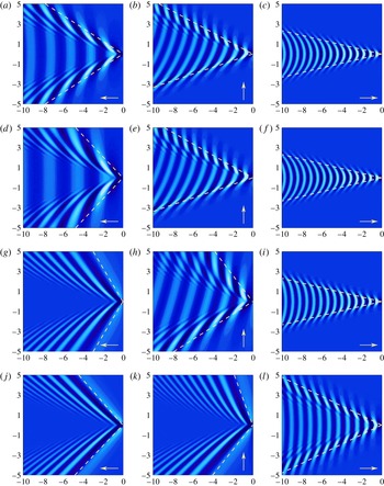
Wave patterns evaluated from the far-field expression (4.1), for different water depths and angles
 ${\it\beta}$
of ship motion relative to the shear current (a,d,g,j)
 ${\it\beta}=0$
, (b,e,h,k)
 ${\it\beta}={\it\phi}/2$
, (c,f,i,l)
 ${\it\beta}={\it\phi}$
. Length scales are in units of
 $2{\rm\pi}bFr^{2}$
. In all graphs,
 $Fr=0.5$
and
 $Fr_{\mathit{s}}=0.5$
. A comparison with figure 5 shows that (g,j) and (k) show supercritical situations. Arrows indicate direction of shear flow in the system where the surface is at rest (see figure 1). (a–c)
 $Fr_{h}^{2}=0$
; (d–f)
 $Fr_{h}^{2}=0.4$
; (g–i)
 $Fr_{h}^{2}=0.8$
; (j–l)
 $Fr_{h}^{2}=1.2$
.

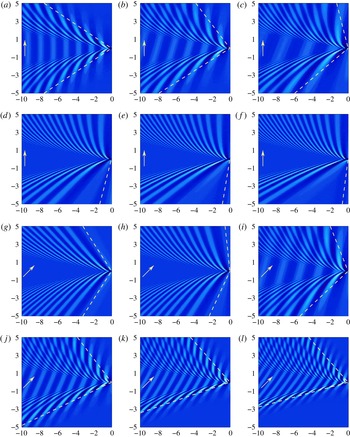
Increasing the shear
 $S$
(and therefore
 $Fr_{\mathit{s}}$
) can cause transition from subcritical to supercritical situation (a–f) or from supercritical to subcritical (g–l) depending on the value of
 $Fr_{h}$
and
 ${\it\beta}$
. In deep waters (
 $Fr_{h}=0$
) only the former transition is possible. In all graphs
 $Fr=0.8$
. Arrows indicate direction of shear flow in the system where the surface is at rest (see figure 1): (a)
 $Fr_{s}=0$
; (b)
 $Fr_{s}=0.5$
; (c)
 $Fr_{s}=0.75$
; (d)
 $Fr_{s}=1.0$
; (e)
 $Fr_{s}=1.25$
; (f)
 $Fr_{s}=1.5$
; (g)
 $Fr_{s}=0$
; (h)
 $Fr_{s}=0.5$
; (i)
 $Fr_{s}=075$
; (j)
 $Fr_{s}=1.0$
, (k)
 $Fr_{s}=1.25$
; (l)
 $Fr_{s}=1.5$
; (a–f)
 $Fr_{h}^{2}=0.8$
,
 ${\it\beta}={\it\pi}/2$
: subcritical to supercritical when
 $Fr_{s}$
increases, (g–l)
 $Fr_{h}^{2}=1.2$
,
 ${\it\beta}=3{\it\pi}/4$
: supercritical to subcritical when
 $Fr_{s}$
increases.

The effect of varying depth on the ship waves is illustrated in figure 9 where the wave field is shown for different values of
 $Fr_{h}^{2}$
when
 $Fr$
and
 $Fr_{\mathit{s}}$
are held constant at moderate values. The values of
 $H$
for each row (a–l) are
 $\infty ,1.6,0.8$
and
 $0.53$
. As the depth decreases the waves for
 ${\it\beta}=0$
(upstream) and
 ${\it\beta}={\rm\pi}/2$
(side-on) both become supercritical, with transverse waves disappearing. The presence of the sea bed is felt most strongly for upstream ship motion (
 ${\it\beta}=0$
), whereas for downstream ship motion (
 ${\it\beta}={\rm\pi}$
) the effect of finite depth only becomes noticeable for the largest
 $Fr_{h}$
, when the wake goes from being made up purely of transverse waves to also showing diverging contributions as well as a wider Kelvin angle. The waves following the downstream-going source are helped along by the current, shortening the wavelength required for transverse waves’ velocity to equal that of the source. A plane wave is affected by the sea floor only if depth is less than roughly half a wavelength, and due to the shortened wavelength, at
 ${\it\beta}={\rm\pi}$
the sea bed only begins to be felt at values of
 $Fr_{h}^{2}$
which are supercritical in the absence of shear.
That a shear current can cause transition from subcritical to supercritical waves when the shear
 $S$
is increased was already shown by Ellingsen (Reference Ellingsen2014b
). However, as figure 5 shows, at finite depth it is also possible to effect the opposite transition by increasing the shear. We illustrate this in figure 10. Figure 10(a–f), the normal transition is seen from sub to supercritical when
 $S$
is increased with other quantities constant (in non-dimensional terms,
 $Fr_{\mathit{s}}$
is increased with constant
 $Fr_{h}$
and
 $Fr$
). Here the direction of motion is
 ${\it\beta}={\rm\pi}/2$
and
 $H\approx 0.31$
, and
 $Fr=0.5$
. Now changing the direction of travel and water depth slightly, to
 ${\it\beta}=3{\rm\pi}/4$
and
 $H=0.21$
at the same source velocity (same
 $Fr$
), creates the opposite situation; now the waves go from supercritical to subcritical as the shear is increased through the same values. It is possible in the latter situation for the waves to become supercritical once more for even higher
 $Fr_{\mathit{s}}$
, but the required values of
 $Fr_{\mathit{s}}$
for the second transition (
 $5.4$
in this example) are so large as to seem unrealistic in practice.
The phenomenon may be understood in terms of dispersion of the waves propagating in the direction of ship motion, i.e. transverse waves, since criticality is the transverse waves becoming too slow to keep up with the source. The effect of finite depth is to limit the phase velocity to values
 ${\leqslant}\!\sqrt{gh}$
isotropically, while the subsurface shear current will advance waves going downstream (as seen from the system where the surface is at rest) and retard upstream-propagating waves. Figure 10(g–l), transverse waves which would otherwise be too slow to contribute to the stationary wake are helped along by the subsurface current, rendering the situation subcritical again when the shear is increased.
5 Wave resistance
We present in this section, for the first time, numerical evaluation and discussion of the wave resistance on a moving pressure source in the presence of shear. We illustrate and discuss the interplay shear and finite depth affect the wave resistance. Calculations of the lateral wave ‘resistance’, present for
 ${\it\beta}\neq 0,{\rm\pi}$
, are reported here for the first time to our knowledge.
Contour considered for the calculation of wave resistance.

In the same vein as (2.20) we can write (2.12) with pressure (2.10) as
 $$\begin{eqnarray}\displaystyle & \displaystyle R=\frac{bp_{0}^{2}}{4{\rm\pi}^{4}{\it\rho}gFr^{2}}\int _{-{\rm\pi}}^{{\rm\pi}}\frac{\text{d}{\it\gamma}}{\cos {\it\gamma}}\lim _{{\it\epsilon}\rightarrow 0^{+}}J({\it\gamma}), & \displaystyle\end{eqnarray}$$
 $$\begin{eqnarray}\displaystyle & \displaystyle J({\it\gamma})=\text{i}\int _{0}^{\infty }\text{d}K\frac{K^{2}\text{e}^{-2(K/2{\rm\pi})^{2}}\tanh KH}{{\it\Gamma}(K,{\it\gamma})+\text{i}{\it\epsilon}{\it\Psi}(K,{\it\gamma})}\equiv \int _{0}^{\infty }\text{d}Kg(K). & \displaystyle\end{eqnarray}$$
 $K_{0}({\it\gamma})$
in (2.25) exists, there is a simple pole which, through the introduction of
 ${\it\epsilon}$
, has been moved slightly off the real
 $K$
axis to a position which is slightly above the axis if
 $\cos {\it\gamma}<0$
and slightly below it if
 $\cos {\it\gamma}>0$
(see the discussion in § 2.4).
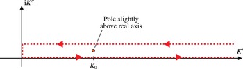
Consider now the case where the pole lies above the axis, and regard the closed contour in the complex
 $K$
plane shown in figure 11. The contour consists of the real
 $K$
axis (the original integration path giving
 $J({\it\gamma})$
) and a horizontal path parallel with the real axis but just far enough above to enclose the pole into the contour. While the quantity
 $R$
is real by construction, a finite value of
 ${\it\epsilon}$
introduces a small imaginary part which vanishes as
 ${\it\epsilon}\rightarrow 0$
, so we treat
 $J({\it\gamma})$
as complex. Now note that because the imaginary unit
 $\text{i}$
enters only as a prefactor and in front of
 ${\it\epsilon}$
, the integral along the upper horizontal path (towards the left) equals
 $J^{\ast }({\it\gamma})$
(complex conjugate) plus a correction of order
 ${\it\epsilon}$
. Hence we have by the Cauchy integral theorem that
 $$\begin{eqnarray}\oint \text{d}Kg(K)=2{\rm\pi}\text{i}\mathop{\text{Res}}_{K=K_{0}}g(K)=J({\it\gamma})+J^{\ast }({\it\gamma})=2\,\text{Re}\{J({\it\gamma})\}\overset{{\it\epsilon}\rightarrow 0}{\longrightarrow }2J({\it\gamma}).\end{eqnarray}$$
If the pole is below the axis instead, the argument remains the same while closing the path in the lower half-plane, producing the opposite sign because the pole is now encircled in the negative sense, and we obtain all together
 $$\begin{eqnarray}\displaystyle \frac{R}{R_{0}}=\frac{1}{2Fr^{2}}\int _{-{\rm\pi}}^{{\rm\pi}}\frac{\text{d}{\it\gamma}}{|\cos {\it\gamma}|}\frac{K_{0}^{2}\text{e}^{-K_{0}^{2}/2{\rm\pi}^{2}}\tanh K_{0}H}{{\it\Gamma}^{\prime }(K_{0},{\it\gamma})}{\it\Theta}[\,f_{s}({\it\gamma})-Fr_{h}^{2}\cos ^{2}{\it\gamma}], & & \displaystyle\end{eqnarray}$$
where
 $R_{0}=bp_{0}^{2}/(2{\rm\pi}^{3}{\it\rho}g)$
, and the
 ${\it\Theta}$
function again ensures inclusion only of
 ${\it\gamma}$
for which
 $K_{0}({\it\gamma})$
exists (
 $f_{s}({\it\gamma})$
was defined in (2.22d
)). For comparison with Benzaquen et al. (Reference Benzaquen, Darmon and Raphaël2014) we plot the quantity
 $R/R_{0}$
which corresponds to the function
 $f$
in their equation (18). (Our result is a factor
 $2$
greater than that of Benzaquen et al. (Reference Benzaquen, Darmon and Raphaël2014) for comparable parameters; the latter reference seems to lose this factor somewhere between their equations (16) and (18).) The same result could be obtained by bypassing the pole on the real axis with a small semicircle, above or below as appropriate.
Hence the wave resistance is given by the pole at
 $K_{0}$
only, which is in fact physically obvious: only waves which satisfy the dispersion relation
 $K=K_{0}({\it\gamma})$
are allowed to propagate towards infinity and thereby remove energy from the source by way of wave resistance.
In his classical analysis nearly a century ago, Havelock (Reference Havelock1922) showed that for an axisymmetric pressure travelling in water of finite depth so that
 $H$
was of order
 $1$
, the wave resistance showed a clear peak at a velocity just below the critical velocity
 $\sqrt{gh}$
, and decreased rapidly for velocities higher than this. We observe the same trend at shallow and intermediate depth also in the presence of shear, while for
 $H\gtrsim 1$
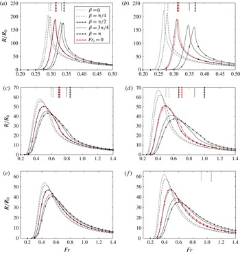
the critical Froude number becomes of little consequence to the wave resistance. Wave resistance is calculated for three different depth (
 $H=0.1,0.5$
and
 $\infty$
) and shown in figure 12 for different directions of motion and increasing values of shear, parameterised through
 $Fr_{Sb}$
defined in (3.2).
The importance of the critical velocity to wave resistance in shallow water, but not in deep water, can be understood from considerations of dispersion. In deep water there is strong dispersion which causes a gradual transition from a wake dominated by transverse waves propagating along the direction of ship motion, to diverging waves propagating almost normal to the direction of motion. Since wave resistance equals the rate at which forward momentum is imparted to the waves, transverse waves must contribute more to wave resistance than a diverging wave of the same absolute momentum but directed almost normal to the ship’s motion. For this reason deep water wave resistance naturally peaks at a value of
 $Fr$
corresponding to the increasing importance of diverging waves. If the critical velocity occurs for a value of
 $Fr$
where transverse waves are still strongly present, however, wave resistance experiences a sudden drop near the critical value because transverse waves vanish. This occurs in shallow water, shown in figure 12(a), and could also occur for very strong shear.
Wave resistance at depth
 $H=0.1$
(a,b),
 $0.5$
(c,d) and
 $\infty$
(e,f) for
 $Fr_{Sb}=0.25$
(a,c,e) and
 $0.5$
(b,d,f). The vertical lines show the critical Froude numbers as given in (3.1).

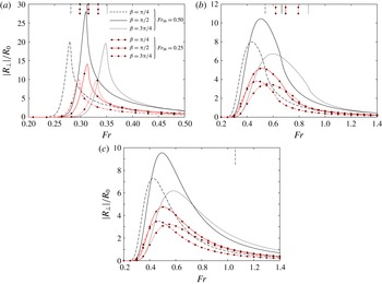
In general the effect of shear upon wave resistance is twofold: to shift the velocity of maximum resistance, and to modify the value of the maximum resistance. For motion against the direction of shear (
 ${\it\beta}=0$
) the peak resistance is higher and is found at smaller values of
 $Fr$
compared to zero shear, while for the source moving with the shear (
 ${\it\beta}={\rm\pi}$
) the peak is lower and shifted to higher
 $Fr$
. In all cases the wave resistance for side-on shear (
 ${\it\beta}={\rm\pi}/2$
) is very close to that found without shear current. All shear effects are stronger for higher values of
 $Fr_{Sb}$
as can be expected. The effect of shear is most dramatic in shallow water, where wave resistance has a sharp peak near the critical Froude number. For vessels operating in the shallows at Froude numbers near the critical, inclusion of the effect of shear seems to be crucial for a realistic calculation of wave resistance.
Firstly, the velocity at which wave resistance peaks is lower for upstream ship motion. In fact, inspection reveals that also other effects of increasing velocity, such as the transition from transverse to diverging wave dominated patterns, occur at lower
 $Fr$
for upstream ship motion (
 ${\it\beta}\sim 0$
) than for downstream (
 ${\it\beta}\sim {\rm\pi}$
). Because waves with an upstream propagation component are retarded by the subsurface shear flow, an upstream-going ship has, in a rough sense, a higher effective velocity as far as the waves are concerned, and effects of increasing velocity are thus shifted to lower values of
 $Fr$
. The opposite is the case for downstream motion.
To understand why wave resistance has a higher peak for upstream motion than for downstream, it may be most instructive to consider the directional dependence of group velocity in the presence of shear, discussed in detail by Ellingsen (Reference Ellingsen2014a
). First, notice that wave resistance peaks at a value of
 $Fr$
where the waves are dominated by transverse waves, i.e. waves propagating approximately in direction
 ${\it\beta}$
. Ship waves have phase velocity which equals the ship velocity along the line of motion, and since gravity waves have a group velocity smaller than their phase velocity, the waves, after being generated (at the bow, say) are left behind as the boat moves forward. A wave can contribute to wave resistance only while it remains in the near field: once left behind its influence is no longer felt by the ship. As discussed by Ellingsen (Reference Ellingsen2014a
) (and illustrated in the context of ring waves), waves travelling upstream have weakened dispersion, and the shear makes the group velocity approach the phase velocity. The time the wave spends in the ship’s near zone is proportional to the difference between group and phase velocity, hence the wave travelling upstream will remain in the ship’s near zone for a longer time, increasing the effect on wave resistance. For the same reason, the effects of transient waves created by the source from manoeuvring, say, can continue to affect the wave resistance for a long time for upstream motion, but are quickly whisked away for downstream motion (Li & Ellingsen Reference Li and Ellingsen2016).
Lateral ‘wave resistance’ for the same values of
 $H,{\it\beta}$
and
 $Fr_{Sb}$
as in figure 12 (for
 ${\it\beta}=0,{\rm\pi}$
the lateral force is zero). The vertical lines show the critical Froude numbers as given in (3.1). The absolute value of
 $R_{\bot }$
is shown; for
 $0\leqslant {\it\beta}\leqslant {\rm\pi}$
,
 $R_{\bot }\leqslant 0$
. (a)
 $H=0.1$
, (b) 0.5, (c)
 $\infty$
.

For all wave resistance calculations it must be noted that wave resistance depends on the shape of the wave source, and the calculations herein, performed for a circular source, is only an illustration and rough indication of the effect of shear upon the wave resistance on a particular hull. The methodology can however be applied to more realistic shapes, at the cost of introducing further parameters.
5.1 Lateral wave ‘resistance’
Now consider the lateral ‘wave resistance’
 $R_{\bot }$
which is calculated exactly like
 $R$
was above, using (2.14) while noting that
 $(\mathbf{e}_{z}\times \boldsymbol{V})\boldsymbol{\cdot }\boldsymbol{k}=kV\sin {\it\gamma}$
,
 $$\begin{eqnarray}\frac{R_{\bot }}{R_{0}}=\frac{1}{2Fr^{2}}\int _{-{\rm\pi}}^{{\rm\pi}}\text{d}{\it\gamma}\frac{\tan {\it\gamma}}{|\!\cos {\it\gamma}\!|}\frac{K_{0}^{2}\text{e}^{-K_{0}^{2}/2{\rm\pi}^{2}}\tanh K_{0}H}{{\it\Gamma}^{\prime }(K_{0},{\it\gamma})}{\it\Theta}[\,f_{s}({\it\gamma})-Fr_{h}^{2}\cos ^{2}{\it\gamma}].\end{eqnarray}$$
The lateral force is plotted in figure 13 for the same values of
 $H$
as used in figure 12. Just like the standard wave resistance, the lateral component also tends to pull the source in the direction where the wave field is strongest, i.e. downstream (as seen from the system where the undisturbed water surface is at rest). The lateral force behaves more or less like the wave resistance as a function of parameters, but is smaller in magnitude. Its maximum value is when the current is approximately side on (
 ${\it\beta}\sim {\rm\pi}/2$
), in which case its value can amount to about 10–20 % of the value of the corresponding no-shear wave resistance when the shear is strong (
 $Fr_{Sb}\sim 1$
).
6 Further discussion and concluding remarks
We have presented a comprehensive theory for linear ship waves on a shear current of uniform vorticity, including the effects of finite depth. A finite water depth and non-zero vorticity each affect the dispersion of the water waves, and the resulting pattern is governed by the two effects in subtle combination. In particular, the phenomenon of a critical velocity at which the wake becomes very broad and above which transverse waves vanish, can be caused by either finite depth or non-zero shear, and in the presence of both the behaviour is intricate.
We derive an explicit formula for the critical velocity for our system as a function of two different Froude numbers (with respect to water depth, and an ‘intrinsic Froude number’) and the angle between current and the source’s line of motion. The phenomenon may be fully understood in terms of dispersion of the waves propagating in the direction of ship motion, i.e. transverse waves, since criticality is the transverse waves becoming too slow to keep up with the source. The effect of finite depth is to limit the phase velocity to values
 ${\leqslant}\!\sqrt{gh}$
isotropically, while the subsurface shear current will advance waves going downstream (as seen from the system where the surface is at rest) and retard upstream-propagating waves. While it was previously shown that increasing the shear strength in deep water could cause transition from sub to supercritical waves (Ellingsen Reference Ellingsen2014b
), in the presence of finite depth, increasing shear strength can also cause the opposite transition for mainly downstream ship motion.
It is a general observation that the presence of a subsurface shear current in a system where the surface is at rest will tend to alter the ‘effective velocity’ of the ship (in a rough sense) relative to the water as far as the waves are concerned. While this notion provides a rough prediction of some qualitative effects of shear upon various aspects of ship waves in shear conditions, it cannot capture the full picture since the dispersion properties of waves in the presence of shear have a subtle directional dependence.
A source generating ship waves will feel a resistance force because waves carry energy away from the source. In the presence of a shear current there will in general also be a lateral component to this force, because the wake is asymmetrical about the ship’s line of motion unless its angle with the shear current is exactly
 $0$
or
 ${\rm\pi}$
. We derive formulae for both the normal and lateral wave resistance force and analyse its dependence on the source velocity (or Froude number
 $Fr$
) for different amounts of shear and different directions of motion. For a circular source the well-known dependence of wave resistance
 $R$
on Froude number is observed –
 $R$
rises to a maximum value before falling off again at higher
 $Fr$
– and the role of the shear current is twofold. Firstly, the velocity of maximum wave resistance,
 $Fr_{max}$
, is lowered for directions moving the source up against the shear, but increased when the motion has a component downstream with the shear (as seen from a system at which the surface is at rest). Secondly the maximum wave resistance is increased for directions against the shear, and decreased for downstream directions.
The lateral ‘wave resistance’ behaves much the same way as a function of Froude number, it is maximal when the current is approximately normal to the direction of motion, and tends to zero for directions directly upstream or downstream.
Appendix A. Details of path integration
In this appendix may be found details of the calculation of path integral
 $I({\it\gamma})$
from (2.20)
A.1 Contribution from the pole
The position of the pole in the integrand of
 $I({\it\gamma})$
is now at
 $K_{pole}=K_{0}-\text{i}{\it\epsilon}F(K_{0},{\it\gamma})$
where
 $$\begin{eqnarray}F(K_{0},{\it\gamma})=\frac{{\it\Psi}(K_{0},{\it\gamma})}{{\it\Gamma}^{\prime }(K_{0},{\it\gamma})}=\frac{2K_{0}Fr^{2}\cos {\it\gamma}+Fr_{\mathit{s}}\cos ({\it\gamma}+{\it\beta})\tanh (K_{0}H)}{Fr^{2}\cos ^{2}{\it\gamma}-f_{s}({\it\gamma})H\,\text{sech}^{2}(K_{0}H)},\end{eqnarray}$$
where
 ${\it\Gamma}^{\prime }(K,{\it\gamma})=\partial {\it\Gamma}(K,{\it\gamma})/\partial K$
. The key property of
 $F(K_{0},{\it\gamma})$
is its sign, which determines which side of the real
 $K$
axis the pole lies. To wit, we note that in order for the pole to lie inside the contour
 ${\it\Lambda}$
,
 $F$
and
 $\cos ({\it\gamma}-{\it\phi}_{{\it\beta}})$
must have opposite signs. It is also necessary that
 $K_{0}({\it\gamma})>0$
as discussed above. If we assume that for some
 ${\it\gamma}$
a solution
 $K_{0}({\it\gamma})>0$
exists, we can use definition (2.25) to write
 $$\begin{eqnarray}F(K_{0},{\it\gamma})=\frac{f_{s}({\it\gamma})+1}{Fr^{2}\cos ^{3}{\it\gamma}}\frac{2\sinh ^{2}{\it\varkappa}}{\sinh 2{\it\varkappa}-2{\it\varkappa}}\end{eqnarray}$$
with
 ${\it\varkappa}=K_{0}({\it\gamma})H$
. It follows from the criterion (3.4) that for
 $K_{0}({\it\gamma})>0$
to exist it is necessary that
 $f_{s}({\it\gamma})>0$
. Moreover one easily ascertains that
 $2\sinh ^{2}{\it\varkappa}/(\sinh 2{\it\varkappa}-2{\it\varkappa})$
is a positive function of
 ${\it\varkappa}$
for all
 ${\it\varkappa}>0$
. In other words,
 $Sg\,[F(K_{0},{\it\gamma})]=Sg\,(\cos {\it\gamma})$
, provided
 $K_{0}({\it\gamma})>0$
(
 $Sg\,$
is the signum function). Hence the pole lies inside the closed contour provided
 $\cos {\it\gamma}$
and
 $\cos ({\it\gamma}-{\it\phi}_{{\it\beta}})$
have opposite signs, i.e.
 $\cos {\it\gamma}\cos ({\it\gamma}-{\it\phi}_{{\it\beta}})<0$
.
Hence we may write using the Cauchy integral theorem, noting that the pole is encircled in the positive sense if
 $\cos ({\it\gamma}-{\it\phi}_{{\it\beta}})>0$
and vice versa,
 $$\begin{eqnarray}\displaystyle \oint _{{\it\Lambda}}\text{d}Kf(K,{\it\gamma}) & \hspace{-2.0pt}=\hspace{-2.0pt} & \displaystyle 2{\rm\pi}\text{i}{\it\Theta}(K_{0}){\it\Theta}[-\!\cos ({\it\gamma}-{\it\phi}_{{\it\beta}})\cos {\it\gamma}]Sg\,[\cos ({\it\gamma}-{\it\phi}_{{\it\beta}})]\mathop{\text{Res}}_{K=K_{pole}}\left\{f(K)\right\}\nonumber\\ \displaystyle & \hspace{-2.0pt}=\hspace{-2.0pt} & \displaystyle I({\it\gamma})-I_{s.d.}({\it\gamma})-I_{conn.}({\it\gamma})\end{eqnarray}$$
or, noting that
 $Sg\,[\cos ({\it\gamma}-{\it\phi}_{{\it\beta}})]=-Sg\,[\cos {\it\gamma}]$
if the pole contributes,
 $$\begin{eqnarray}\displaystyle I({\it\gamma})=I_{s.d.}({\it\gamma})+I_{conn.}({\it\gamma})-2{\rm\pi}\text{i}{\it\Theta}(K_{0}){\it\Theta}[-\!\cos ({\it\gamma}\!-\!{\it\phi}_{{\it\beta}})\cos {\it\gamma}]Sg\,[\cos {\it\gamma}]\mathop{\text{Res}}_{K=K_{\mathit{pole}}}\left\{f(K)\right\}\!, & & \displaystyle \nonumber\\ \displaystyle & & \displaystyle\end{eqnarray}$$
where the Heaviside functions
 ${\it\Theta}$
enforce the criteria for the pole being inside the integral, and the contributions from the parts of the path are
 $$\begin{eqnarray}\displaystyle & \displaystyle I_{s.d.}({\it\gamma})=\int _{|{\it\Xi}|}^{\infty }\text{d}Kf(K+\text{i}{\it\Xi},{\it\gamma}), & \displaystyle\end{eqnarray}$$
 $$\begin{eqnarray}\displaystyle & \displaystyle I_{conn.}({\it\gamma})=(1\pm \text{i})\int _{0}^{|{\it\Xi}|}\text{d}Kf[(1\pm \text{i})K,{\it\gamma}]. & \displaystyle\end{eqnarray}$$
 ${\it\Xi}=2{\rm\pi}^{2}X\cos ({\it\gamma}-{\it\phi}_{{\it\beta}}),$
whereby
 $K_{s.d.}=K+\text{i}{\it\Xi}$
. The sign to be taken in (A 6) is the sign of
 ${\it\Xi}$
. Thus, by (A 4) the integral
 $I({\it\gamma})$
can be written in terms of a steepest descent integral, a connection path, and possibly the residue of the pole.
A.2 Asymptotic fall off of path integrals
Consider now large distances
 $X$
to consider asymptotic behaviour. We presume therefore in the following that
 $|{\it\Xi}|\rightarrow \infty$
.
Inserting
 $K_{s.d.}$
, the steepest descent integral becomes (
 ${\it\epsilon}$
is only of interest inasmuch as it moves the pole off the real
 $K$
axis, and can be set to zero in the following)
 $$\begin{eqnarray}I_{s.d.}=\text{e}^{-{\it\Xi}^{2}/2}\int _{|{\it\Xi}|}^{\infty }\text{d}K\frac{K_{s.d.}\text{e}^{-(K/2{\rm\pi})^{2}}\tanh (K_{s.d.}H)}{{\it\Gamma}(K_{s.d.},{\it\gamma})}.\end{eqnarray}$$
Numerical inspection reveals that the integral in (A 7) is a nearly periodic function of
 ${\it\Xi}$
with sharp peaks at
 ${\it\Xi}H=(n+1/2){\rm\pi}$
(
 $n=1,2,3,\ldots$
) and which is everywhere of order unity. The prefactor
 $\exp (-{\it\Xi}^{2}/2)$
and the fact that the integral starts at the (already very large) lower limit
 $|{\it\Xi}|$
ensure that the integral is exponentially small as
 ${\it\Xi}\rightarrow \infty$
.
Next considering
 $I_{conn.}$
, we write
 $$\begin{eqnarray}I_{conn.}=(1\pm \text{i})^{2}\int _{0}^{|{\it\Xi}|}\text{d}K\frac{K\text{e}^{-2\text{i}K^{2}/(2{\rm\pi})^{2}}\tanh (1\pm \text{i})KH}{{\it\Gamma}[(1\pm \text{i})K]}\text{e}^{(\text{i}{\it\Xi}-|{\it\Xi}|)K/2{\rm\pi}^{2}}.\end{eqnarray}$$
Asymptotic analysis of this integral in itself is straightforward, by noting that its main contribution comes from small values of
 $K$
of order
 $1/{\it\Xi}$
. However, the resulting expression yields a non-integrable function of
 ${\it\gamma}$
, so an asymptotic analysis of the full double integral is necessary. We satisfy ourselves by performing the integral numerically and find that the contribution to
 ${\it\zeta}$
from the connection integral falls off slightly faster than
 $X^{-1}$
as
 $X\rightarrow \infty$
(most likely a logarithmic contribution is involved). The surface deformation in the far field falls off as
 $X^{-1/2}$
(e.g. Ellingsen Reference Ellingsen2014b
) as is required by energy conservation, hence the connection integral is part of the near field.
We have shown that
 $I_{s.d.}$
and
 $I_{conn.}$
fall off faster than the far field solution when
 $X\rightarrow \infty$
. More detailed asymptotic analysis of
 $I_{s.d.}$
and
 $I_{conn.}$
is of course possible, yet given the complexity of the integrals involved and the fact that our primary interest is the far field, we shall be content here with this brief treatment.
Appendix B. Note on the use of the Sokhotski–Plemelj theorem
In the literature, the so-called Sokhotski–Plemelj theorem has sometimes been used in order to extract the far-field contribution to the wave field (Raphaël & de Gennes Reference Raphaël and de Gennes1996; Benzaquen et al. Reference Benzaquen, Darmon and Raphaël2014; Darmon et al. Reference Darmon, Benzaquen and Raphaël2014; Ellingsen Reference Ellingsen2014b ). We show here that while the correct far field can be obtained this way in parts of the plane (modulo a prefactor of 2 for the wave amplitude), what is obtained is in fact a combination of the far field allowed by the radiation condition and the spurious ‘far field’ which is physically illegal because it corresponds to waves travelling from future to past (or alternatively: originate at infinity and converge at the source).
Comparison of wave fields
 ${\it\zeta}(\boldsymbol{x})$
calculated using (a) full expression from (2.8) with a small, non-zero value of
 ${\it\epsilon}$
, (b) the Sokhotksy–Plemelj expression
 ${\it\zeta}_{S{-}P}$
(with integration range
 $-{\rm\pi}<{\it\gamma}<{\rm\pi}$
), (c) our far-field expression
 ${\it\zeta}_{\mathit{f.f.}}$
from (4.1), and (d) the combination
 $2{\it\zeta}_{S\text{-}P}-{\it\zeta}_{\mathit{f.f.}}$
. Parameters are
 $Fr=Fr_{\mathit{s}}=0.8$
,
 $Fr_{h}=0$
, and
 ${\it\beta}={\rm\pi}/2$
in (a–d).

Let us consider the surface deformation
 ${\it\zeta}$
and consider the case of deep water for simplicity (the principle is the same for finite water depth), in which case
 ${\it\zeta}$
from (2.8) can be written on the general form
 $$\begin{eqnarray}{\it\zeta}={\it\zeta}_{0}\int _{-{\rm\pi}}^{{\rm\pi}}\text{d}{\it\gamma}\lim _{{\it\epsilon}\rightarrow 0}\int _{0}^{\infty }\frac{\text{d}k\,f(k)}{k-k_{0}-\text{i}{\it\epsilon}{\it\phi}},\end{eqnarray}$$
where
 ${\it\zeta}_{0}$
is a constant and
 ${\it\phi}$
is a function of
 $(k,{\it\gamma})$
which can take either sign. We now wish to evaluate just the far-field contribution to the
 $k$
-integral. The procedure of, e.g. Darmon et al. (Reference Darmon, Benzaquen and Raphaël2014) is now to use the so-called Sokhotski–Plemelj (SP) theorem to evaluate the contribution from the simple pole at
 $k=k_{0}$
, which is then identified as the far field.
The SP theorem is very simple to derive and results from simply multiplying the integrand by
 $k-k_{0}+\text{i}{\it\epsilon}{\it\phi}$
in numerator and denominator and splitting into two terms:
 $$\begin{eqnarray}\displaystyle & & \displaystyle \hspace{-20.00003pt}\lim _{{\it\epsilon}\rightarrow 0}\int _{0}^{\infty }\text{d}k\frac{f(k)}{k-k_{0}-\text{i}{\it\epsilon}{\it\phi}}=\text{i}{\rm\pi}\lim _{|{\it\phi}|{\it\epsilon}\rightarrow 0}\int _{0}^{\infty }\text{d}k\frac{{\it\epsilon}|{\it\phi}|f(k)}{{\rm\pi}[(k-k_{0})^{2}+{\it\epsilon}^{2}{\it\phi}^{2}]}Sg\,({\it\phi})\nonumber\\ \displaystyle & & \displaystyle \hspace{-20.00003pt}\qquad +\lim _{{\it\epsilon}\rightarrow 0}\int _{0}^{\infty }\text{d}k\frac{(k-k_{0})^{2}}{(k-k_{0})^{2}+{\it\epsilon}^{2}{\it\phi}^{2}}\frac{f(k)}{k-k_{0}}=\text{i}{\rm\pi}Sg\,({\it\phi}_{0})f(k_{0})+\mathscr{P}\int _{0}^{\infty }\text{d}k\frac{f(k)}{k-k_{0}},\end{eqnarray}$$
where
 $\mathscr{P}$
denotes the principal value, and
 ${\it\phi}_{0}={\it\phi}(k_{0},{\it\gamma})$
. The last form is obtained by noting that
 ${\it\varepsilon}/{\rm\pi}(x^{2}+{\it\varepsilon}^{2})\rightarrow {\it\delta}(x)$
as
 ${\it\varepsilon}\rightarrow 0^{+}$
, and recognising a definition of the principal value. The theorem is of course valid, but the potential danger lies in now identifying the first term in the last form of (B 2), proportional to
 $f(k_{0})$
as the far field, and the second term as the near field.
We can see this most easily by regarding the term which becomes the
 ${\it\delta}$
-function, purportedly the far-field contribution according to the SP procedure. In a slight change of notation from the above this term alone can be written
 $$\begin{eqnarray}\lim _{{\it\epsilon}\rightarrow 0}\int _{0}^{\infty }\text{d}k\frac{\text{i}{\it\epsilon}{\it\phi}f(k)}{(k-k_{0})^{2}+{\it\epsilon}^{2}{\it\phi}^{2}}=\lim _{{\it\epsilon}\rightarrow 0}\int _{0}^{\infty }\text{d}k\frac{1}{2}\left[\frac{f(k)}{k-k_{0}-\text{i}{\it\epsilon}{\it\phi}}-\frac{f(k)}{k-k_{0}+\text{i}{\it\epsilon}{\it\phi}}\right],\end{eqnarray}$$
where we have expanded in partial fractions. Now comparing with the original, full expression (B 1) we see that the purported ‘far-field’ solution is in fact half the full wave field minus half of the wave field obtained from swapping the sign of
 ${\it\epsilon}$
, i.e. exactly the waves which the radiation condition is supposed to exclude.
Apart from the factor
 $1/2$
, the situation is not too serious, because the real wake in (B 1) lies behind the ship, whereas the spurious ‘wake from the future’ in the second term of (B 3) lies in front of it. The situation is illustrated in figure 14 Indeed the ‘far-field’ wave expressions in Darmon et al. (Reference Darmon, Benzaquen and Raphaël2014), Ellingsen (Reference Ellingsen2014b
) give waves also antisymmetrically in front of the ship which must be manually removed (for example by simply not plotting them). The procedure employed in our § 2.4, while somewhat more elaborate, avoids this problem.