

Introduction
The practice of precision agriculture (PA) requires identifying fairly homogeneous areas for site-specific management. This could be achieved by interpolation of relevant soil properties between sample points. However, this approach is expensive since it requires a large number of points, evenly distributed and sampled at intervals short enough to allow for spatial dependence between them. Digital elevation models (DEM) of high-resolution can be produced from images obtained from unmanned aerial vehicles (UAV). Such DEMs can be used to create a terrain classification based on small topographic differences within plots. The terrain classes could be used to delineate areas for site-specific management, provided they are related to changes in soil conditions.
Digital soil mapping includes different methods to interpolate for spatial prediction (Hengl, Reference Hengl and Evans2009). Among these methods, linear statistical models such as kriging, environmental correlations, Bayesian models and hybrid models require that the input data accomplish with strict statistical stationary assumptions of the interpolated variable. Specifically, kriging and its derivatives are based on the theory of regionalized variables. Its objective is to predict the values at non-sampled points, based on the model of a stochastic stationary process, for which it is necessary that the point values are spatially autocorrelated (Valera, Reference Valera2015). The standard version is called ordinary kriging and the predictions are based on equation (1):
 $$Z\left( s \right)\,{\equals}\,\mu {\plus}{\epsilon}'\left( s \right)$$
where the value of Z at a given point is equal to a stationary constant function (global mean, μ) plus the random component (ε') of spatially correlated variation.
Grids of interpolated values of soil properties can be combined into a single map to produce of management units for PA. Such management units could also be produced by means of a predictive model of soil variation based on a set of soil data recorded at known locations, and a set of environmental covariates derived from a high-resolution DEM. The most adequate methods to model the soil variation to this aim appear to be those which allow working with uncertain and noisy phenomena, given the rather complex relationships between environmental variables and soil properties. These methods include unsupervised classifications based on artificial neural networks (ANN) (e.g. Zhu, 2000; Fidêncio et al., 2001; Zhao et al., 2009, Viloria et al., Reference Viloria, Viloria-Botello, Pineda and Valera2016), fuzzy sets (e.g. Lark, 1999; Zhu et al., 2001; Beucher et al., 2014; Akumu et al., 2015), or a combination of them (e.g. Viloria et al., Reference Viloria, Viloria-Botello, Pineda and Valera2016). In particular, the Fuzzy Kohonen Clustering Network (FKCN) is a neuro-fuzzy network (Bezdeck et al., Reference Bezdek, Tsao and Pal1992; Viloria, Reference Viloria2007) that generates representations of similarity values or functions of neuro-fuzzy memberships in raster format, with expressions of membership values to each class (between 0 and 1). Under this approach, the value of an environmental covariate of a given pixel can be assigned to more than one class or management unit. Grades of class assignment are referred to as a graded.
Two different maps of potential management units were created in this work by means of FKCN. The first map was based on a classification of interpolated values of soil variables, whereas the second map was created by a classification of terrain attributes derived from a DEM produced from UAV images. Both maps represent soil-landscape relationships and subdivide the area into more homogeneous units. In previous works related to generation of management units for PA, efficiency to delineate such units by one methodology or another has been evaluated (Ortega et al., 2007; Song et al., Reference Song, Wang, Huang, Liu, Yan and Pu2009; Davatgar et al., Reference Davatgar, Neishabouri and Sepaskhah2012; Tripathi et al., Reference Tripathi, Nayak, Shahid, Lal, Gautama, Raja, Mohanty, Kumar, Panda and Sahoob2015). Nevertheless, the possibility of using other input variables different to soil properties or crop yield has not been evaluated. Soil or yield-related variables may have a bias derived from the sampling distance, the behavior of the variable or the crops management. In addition, sampling in a systematic way involves investment of time and money, which is why the variables generated by remote sensing are increasingly used (Song et al., Reference Song, Wang, Huang, Liu, Yan and Pu2009; Chang et al., Reference Chang, Zhang, Zhu, Ge, Li and Liu2014). The objective of this research is to compare the performance of management units delimited from (a) soil variables and (b) environmental covariates, in order to show whether the last can be used to delineate areas for site-specific management, saving time and money.
Material and methods
Study area
The study area occupies 6 ha and is located in the experimental field of the Faculty of Agronomy of the Central University of Venezuela in Maracay city. The region corresponds to a tropical dry forest climate. The annual average temperature is 25°C, the average annual rainfall is 1,063 mm and the average annual evaporation is 1,080 mm (Agricultural Climatology Service of the Faculty of Agronomy, UCV). The soils of the area were developed on alluvial sediments derived from micaceous schists. In general, the area is covered by intensive crops.
Soil data
Soil sampling was carried out in 50×50 m squares to cover all the variability observed in the area. This distance was selected to take into account the distance of different samples previously made in neighboring areas, where it was indicated that the distance that solves the pattern of variation of the soils is between 61.5 and 100 m (Ovalles and Rey, Reference Ovalles and Rey1994). A total of 86 sampling points were taken. Each sampling point was located in the field with the support of a GPS with a precision of 3 m. At each point a soil sample was taken from the first horizon to determine the content of sand (a, %) and clay (A, %) by the Bouyoucos method, pH in water 1:1 (pH), electrical conductivity (EC, dS/m), soil organic carbon (SOC, %) by the Walkley and Black method, cation exchange capacity (CIC, cmol kg–1) at pH 7 and thickness of the first horizon A (cm).
Statistical analysis
A descriptive statistical analysis was performed to examine the behavior of variables and to identify outliers. According to the procedure proposed by Tukey (Reference Tukey1977), values higher or lower than the external fences of the data distribution were considered as outliers. This method considers observation Y an outlier if: Y<(Q1−1.5 IQR) or Y>(Q3+1.5 IQR), where Q1=lower quartile, Q3=upper quartile, and IQR=(Q3−Q1) is the interquartile range. Additionally, the Kolmogorov-Smirnov normality test was done.
Generation of map of soil variables
Once the normality of the variables was evaluated, their spatial distribution was adjusted to theoretical semivariograms, determining the spatial dependence or range (A1). From the semivariograms, we obtained optimal estimates of regionalized variables at non-sampled sites through ordinary kriging (Webster and Oliver, Reference Webster and Oliver1990), when the variables did not present spatial dependence was represented by the inverse of the distance (IDW). The maps of the different variables were used as input in the FKCN software, in order to generate a map of terrain classes or management units (Tripathi et al., Reference Tripathi, Nayak, Shahid, Lal, Gautama, Raja, Mohanty, Kumar, Panda and Sahoob2015).
Generation of the DEM from UAV images
A 5 m spatial resolution DEM was generated from images taken by an UAV. For that, six control points were used. Six additional points were used to validate the result. The XYZ coordinates of these control points were determined by means of a GPS receiver (MAGELLAN, model Promark 3 with antenna NAP100). The device was configured with a cutting angle or lifting mask over the horizon of 15° and 5 seconds of recording interval. The data obtained were post processed with the software GNSS Solution v. 3.7.50. The mean accuracy of the ground control points, with respect to the known coordinate vertexes, was 2 mm, in XYs and 2 mm in Z.
Environmental covariates
From the DEM, several topographic parameters were derived. Those were called environmental covariates: elevation, slope degree, profile curvature, plan curvature, topographic wetness index, sediment transport index. The environmental covariates correspond to the factors of Jenny’s (Reference Jenny1941), CLORPT equation, and to the multivariate geospatial SCORPAN model, formulated by McBratney et al. (Reference McBratney, Mendonça and Minasny2003). These were used as input parameters for the generation of a map of management units corresponding to soil-landscape relationships. The environmental covariates were computed with SAGA GIS (System for Automated Geoscientists Analyses, v.2.0.8).
Terrain classes or management units
For the grouping of soil variables and environmental covariates, FKCN was applied (Bezdeck et al., Reference Bezdek, Tsao and Pal1992; Viloria, Reference Viloria2007). The procedure consists in entering the input data in ASCII format to generate an array of variables, to train the neural network. For that, learning parameters (number of classes: 3–12, fuzzy exponent (ø): 1.1–1.6, convergence error: 0.0001–0.001, number of iterations: 20-50) must be specified. Then, maps of similarity values of classes are obtained and, finally, the final model or map of management units is generated (Valera, Reference Valera2015).
Validations
The validation of the proposed management units was performed with the values of the soil properties used for the generation of soil property maps using kriging. Later, it was determined whether or not there were significant differences between the proposed units, through the F test (α=0.05) taking into account the value of soil variables. Finally, a test of means was done to establish whether there were differences or similarities between the different units.
Results
The variables that presented spatial dependence were represented by ordinary kriging (clay, SOC and pH), the remaining variables (thickness, cation exchange capacity, electrical conductivity and sand) were represented by the inverse of the distance (IDW).
Selection of the fuzziness coefficient and the number of classes
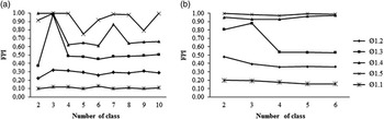
As shown in figure 1, according to the fuzziness performance index (FPI), the optimal number of classes or management units was 4, with a fuzzy exponent (ø) of 1.3, for both, the classes obtained from environmental covariates or those obtained from the soil variables.
Variation of the fuzziness performance index (FPI) with the fuzzy exponent (ø) and the number of classes of land surface to a) soil variables and b) environmental covariates. A combination of ø=1.3 and four classes was chosen as the best option for this study.

Tables 1 and 2 show the centroid values of each class, for both the class map obtained from soil variables and for the class map obtained from environmental covariates. Regarding the classes obtained from the soil variables (Table 1), Class 1 had a higher pH value; Class 2 presented a higher cation exchange capacity and the lowest value of electrical conductivity; Class 3 presented the highest values of soil thickness, soil organic carbon and clay content and the lowest pH values. Class 4 presented the highest value of electrical conductivity.
Centroids of each one the classes generated from soil variables

Centroids of each one the classes generated from environmental covariates.

Table 2 shows the differences between the four proposed management units generated from the environmental covariates. Class 1 was located in the lowest landscape position. It was characterized by being concave to cross sectional or longitudinal curvature, the lowest slope degree and the highest topographic wetness index. Class 2 was located in the highest landscape position and had a cross sectional and longitudinal convex shape. Classes 3 and 4, had a higher slope degree. Class 3 had a longitudinal and cross sectional convex shape, and Class 4 a concave shape in both directions and, therefore, a higher topographic wetness index compared to Class 3.
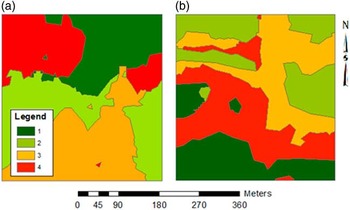
Figure 2 shows the spatial location of the management units obtained from both data sources. It is worth to note that these classes were not analogous. Class 1 of the map obtained from soil variables did not correspond geographically with Class 1 of the map of management units obtained from the environment covariates.
Management units obtained from a) soil variables b) environmental covariates.

Validation
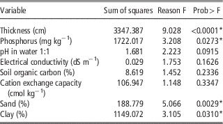
Table 3 shows that there were significant differences between management units only for soil thickness, sand, clay and phosphorus content. The rest of the variables did not show significant differences. The chemical variables did not present significant differences, except phosphorus (Table 3). The reason could be that soils of the study area were developed over sediments from the Güey River, which in turn come from the Las Brisas formation. The phosphorus has a different behavior because the input is mainly from fertilization. Differences in soil thickness, sand and clay content could be attributed to differential deposition occurring in the area, as result of alluvial sedimentation.
Probability of existence of significant differences between the classes generated from the environmental covariates and soil properties.

*Significantly different between each class.
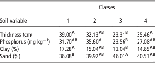
In most cases (Table 4) the soil variables showed that the management units obtained from environmental covariates were correctly delimited. Although each variable showed that at least two classes overlapped, this overlap did not always occur between the same classes. For example, the classes 1 and 2 do not show differences in thickness and phosphorus content, but they show differ in clay and sand content. Classes 2 and 3 show differences in phosphorus content but there are overlaps between classes for the other variables. Accordingly, the obtained management units will probably show differences in the dynamics of water and nutrients in the soil, as well as in the stability of the soil physical structure.
Mean least-squares test for each class and soil variable.

The map generated from the soil variables, as expected, is not the same as the map generated from the environmental variables. Although a large number of samples were taken, there is a bias in generating the final map from these variables, because the appropriate sampling distance is difficult to establish and is different for each variable. Additionally, the values generated between one sampling point and another are the product of interpolation, while that the map generated from the environmental variables have values for each pixel and the establishment or determination of an appropriate sampling distance is not necessary. The results show that the delimitation of management units from environmental covariates may be an alternative for the delimitation of management units or homogeneous zones, as shown by Reyniers et al. (Reference Reyniers, Maertens, Vrindts and De Baerdemaeker2006). However, it is necessary to determine if there is a relationship between these variables and the yield, as suggested by Ortega and Santibáñez (Reference Ortega and Santibáñez2007) and Yao et al. (Reference Rong-Jiang Yao, Yanga, Zhang, Gao, Wang, Hong and Wang2014). The values of clay as centroids in all classes show that the predominant textural class is the franca, Map intends to model the internal variation of a “natural soil body”.
Discussion
The main purpose of generating terrain management units is to subdivide the total area into more homogeneous units that allow site-specific management (Ruß et al., Reference Ruß, Kruse and Schneider2010). However, for a proper subdivision of an area, one must work with the appropriate resolution. So far the solution to model the internal variation of soil bodies has been interpolated by kriging, but this solution is expensive because a large number of point samples of soil are needed. Additionally, sampling is not always done at the proper distance, so it is possible that the map obtained by kriging does not present the detail necessary to divide the studied area into appropriate management units. Generally, kriging is generated from physical, chemical or biological variables that operate at different intensities and at different time space scales, whose values may even be affected by crop management, fertilization, and irrigation (Tripathi et al., Reference Tripathi, Nayak, Shahid, Lal, Gautama, Raja, Mohanty, Kumar, Panda and Sahoob2015). In addition, each soil property has a differential behavior. While the terrain variables derived from the DEM show the existing natural variability of the terrain and a value for each pixel can be derived. The spatial resolution could be a constrain to define areas for site-specific management from terrain variables. However, images taken from UAVs nowadays provide an option to obtain a high resolution DEM at a fairly low cost. In this last case, management units can be generated at low costs and with easy-to-use tools. On the other hand, when using a map obtained by kriging it is not certain that it can be used to predict the value of a soil variable, since this depends on the spacing between samples and the degree of similarity between them, and even it is almost certain that it cannot be used as a framework or guide for another sampling (Webster and Butler, Reference Webster and Butler1976). Finally, the generation of management areas through environmental covariates reduces the number of samples necessary for the delimitation of the areas and those necessary to carry out the planning and cultivation work in the area.
Conclusions
Obtaining terrain classes or management units from environmental covariates seems to be an alternative for the delineation of site-specific management zones in low relief crop areas. For their generation, less time and money are invested compared in comparison to the management units obtained from soil variables. Nevertheless, it is advisable to analyze the relationship between these type of management units and variables such as yield or productivity.
Acknowledgment
This research was funded by the Venezuelan Organic Law for Science and Technology (LOCTI) and the Consejo de Desarrollo Científico y Humanístico (Council of Scientific and Humanistic Development) of the Universidad Central de Venezuela (CDCH-UCV). We are also grateful to the International Centre for Theoretical Physics (Trieste, Italy) for the financial support and fellowships.