
1. Introduction
When a tank partially filled with liquids is subjected to vertical excitation, standing waves, called Faraday waves, are generated on the free surface. This phenomenon was first observed and studied in laboratory by Faraday (Reference Faraday1831), who discovered that resonance occurs when the frequency of vertical external excitation is twice the natural frequency of the liquid. More than one century later, McLachlan (Reference McLachlan1947) obtained the stable and unstable region of the Mathieu equation by using mathematical analysis and Benjamin & Ursell (Reference Benjamin and Ursell1954) found that the governing equation of inviscid Faraday waves is equivalent to the Mathieu equation, from which the stable and unstable regions of Faraday waves can be determined.
From the 1990s, viscous Faraday waves began to be studied extensively and there were many investigations of free surface Faraday waves by theoretical analyses, laboratory experiments and numerical modelling. For example, Bechhoefer et al. (Reference Bechhoefer, Ego, Manneville and Johnson1995) systematically measured the threshold accelerations in exciting the Faraday instability by using a viscous fluid. Cerda & Tirapegui (Reference Cerda and Tirapegui1997, Reference Cerda and Tirapegui1998) derived a new equation for the amplification of surface Faraday waves of a highly viscous fluid in a horizontally homogeneous domain, and they concluded that when the amplitude of excitation acceleration makes the effective acceleration negative, the Rayleigh–Taylor (RT) instability will occur. Lioubashevski, Fineberg & Tuckerman (Reference Lioubashevski, Fineberg and Tuckerman1997) conducted experiments with high-viscosity fluids in a circular cell moving vertically and they came to a similar conclusion that upward acceleration can force the liquid layer to be susceptible to RT instability. In the above works by Cerda & Tirapegui (Reference Cerda and Tirapegui1997, Reference Cerda and Tirapegui1998) and Lioubashevski et al. (Reference Lioubashevski, Fineberg and Tuckerman1997), the Faraday waves were actually the result of RT instability as the external excitation is much larger than gravitational acceleration. Jiang et al. (Reference Jiang, Ting, Perlin and Schultz1996) experimentally analysed mild to steep standing waves generated in a rectangular tank undergoing vertical excitations. They found that increasing the excitation amplitude could lead to period tripling breaking waves in the form of three modes, i.e. sharp crest with breaking, dimpled or flat crest with breaking, and round crest without breaking. Murakami & Chikano (Reference Murakami and Chikano2001) examined standing surface waves of a viscous fluid driven by a vertical harmonic oscillation based on direct numerical simulations of the two-dimensional (2-D) Navier–Stokes equations (NSEs). Jin, Xue & Lin (Reference Jin, Xue and Lin2021) utilised a three-dimensional (3-D) NSEs model and systematically studied resonant Faraday waves with different modes.
Although Faraday waves were first observed on a free surface between air and liquid, they also occur on the interface between two liquids bounded by walls at the top and the bottom. The Atwood number,  $A$, which is the ratio between the density difference and density sum of two fluids, is commonly used to quantify the density difference between two fluids and it is around 1 for an air–liquid system but much smaller for a liquid–liquid system. Faraday waves on the interface between two liquid layers enclosed by horizontal plates are not crucially different from Faraday waves on a free surface, both of which can be described by the Mathieu equation. Wright, Yon & Pozrikidis (Reference Wright, Yon and Pozrikidis2000) numerically simulated the dynamics of 2-D standing waves at the interface between two inviscid fluids with different Atwood number, and it was found that when the conditions of external excitation fell into unstable region, plumes could be developed at moderate values of Atwood number, whereas droplets will be ejected at higher values of Atwood number. In contrast to Faraday waves at the interface between ideal liquids, Kumar & Tuckerman (Reference Kumar and Tuckerman1994) presented linear stability analysis by using Floquet theory in a horizontally homogeneous domain for the interface between two viscous fluids under vertical excitation, which could not be reduced to a system of Mathieu equations for liquids with high viscosity. They concluded that it was necessary to consider the viscous boundary conditions at the top and the bottom of the configuration to obtain a better estimation of the stability threshold if the liquid layers have finite depths. Interface Faraday waves between two immiscible liquids in a cylindrical cell were studied by Tipton & Mullin (Reference Tipton and Mullin2004) and the influence of the volume filling ratio on the bifurcation set in connection to the onset of the fundamental axisymmetric mode was examined. Périnet, Juric & Tuckerman (Reference Périnet, Juric and Tuckerman2009) and Kahouadji et al. (Reference Kahouadji, Périnet, Tuckerman, Shin, Chergui and Juric2015) performed numerical simulations of Faraday waves in three dimensions for two incompressible and immiscible viscous fluids. The NSEs were solved in their model and the front-tracking method was employed for the interface tracking between the two fluids. However, all the Faraday waves mentioned previously occur only on one interface between two fluids. A comprehensive review of Faraday waves and parametric sloshing can be found in Miles & Henderson (Reference Miles and Henderson1990) and Ibrahim (Reference Ibrahim2015).
Faraday waves occurring on both the free surface and the interface between two liquids simultaneously have not been investigated until recently. Faraday instabilities of a liquid drop floating on another more viscous liquid were studied by Pucci et al. (Reference Pucci, Fort, Ben Amar and Couder2011); Pucci, Ben Amar & Couder (Reference Pucci, Ben Amar and Couder2013). They found in their experiment that the displacement of interface is much smaller than that of free surface. Pototsky & Bestehorn (Reference Pototsky and Bestehorn2016) employed an integrated layer model based on the NSEs with long-wave approximation to study the layered thin liquid film with a free upper surface under vertical excitations. The conditions of the in-phase and anti-phase displacements were determined, and the location of the stability threshold of two-layer liquid film was obtained based on numerical simulations. In addition, by placing the heavier liquid on top of the lighter liquid, they found that when the acceleration of excitation is large, the development of RT instability was suppressed. Li, Li & Liao (Reference Li, Li and Liao2018a); Li et al. (Reference Li, Li, Liao and Chen2018b) conducted experiments on two coupled Faraday waves in a Hele-Shaw cell under periodic vertical vibration. They observed that the upper surface vibrated vertically whereas the lower surface oscillated horizontally with the same wave height. They also discussed the influence of the depth of upper and lower liquids on the standing waves on both free surface and interface. Zhao, Dietzel & Hardt (Reference Zhao, Dietzel and Hardt2019) investigated the Faraday instability of an immiscible two-layer system with the bottom film much thinner than the top layer, which could be also viewed as a single-layer liquid with a Navier-slip boundary on the bottom. However, the full two-layer system can capture the flow properties inside the thin film, which could not be fully reflected in a single-layer model.
So far there has been no report on the possible secondary interface instabilities that may occur during the resonant Faraday waves of two-layer liquids with free surface, considering the interaction between free surface and liquid–liquid interface. In addition, systematic studies of resonant Faraday waves on both free surface and interface between two liquids under different vertical excitations are less reported. On the other hand, some engineering systems are concerned with multiple-layer Faraday waves and their interface instabilities. For example, a wash-tank or a separator on a floating production storage and offloading (FPSO) unit may contain water and crude oil, thus forming a two-layer liquid system with free surface. A common sea state may induce resonant Faraday waves with breaking free surface or secondary interface instabilities, which may pose a threat to the stability of the tank on FPSO or induce mixing of the layered water and crude oil, both of which should be avoided in practice.
In this study, the phenomena of upper layer resonance (free surface), lower layer resonance (liquid interface) and both layer resonances are investigated by conducting laboratory experiments and numerical modelling. We focus on the secondary surface and interface instabilities induced by the Faraday waves. In § 2, we review the numerical model called NEWTANK that is utilised to study the Faraday waves in a two-layer liquid system with free surface under vertical periodic excitations. A multilayer volume-of-fluid (ML-VOF) method (Liu et al. Reference Liu, Lin, Xue, Cheng and Lian2021) is employed to track both free surface and the interface between different liquids simultaneously. The experimental apparatus is described in § 3, followed by a systematical study on resonant Faraday waves and secondary surface and interface instability in § 4. The threshold for generating secondary interface instabilities of RT type or Kelvin–Helmholtz (KH) type is analysed and discussed, with the introduction of a new dimensionless parameter to define the incipient criterion of RT interface instability. Conclusions are drawn in § 5.
2. Mathematical model and numerical implementation
2.1. Governing equations
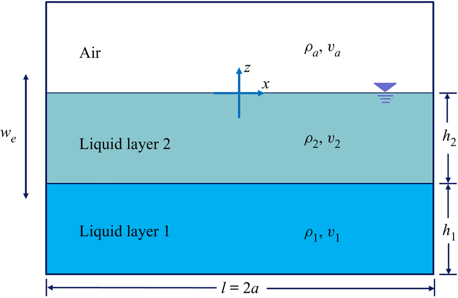
The spatially filtered NSEs are employed as the governing equations of the numerical model NEWTANK (Liu & Lin Reference Liu and Lin2008) in this study, under the assumption of incompressible fluid. In addition, the coordinate system is fixed on a moving tank with the non-inertial reference frame following the tank motion. The resulting continuity equation and NSEs are
 \begin{gather} \frac{\partial \bar{u}_i}{\partial x_i}=0, \end{gather}
 \begin{gather} \frac{\partial \bar{u}_i}{\partial t}+\bar{u}_j\frac{\partial \bar{u}_i}{\partial x_j}={-}\frac{1}{\rho}\frac{\partial \bar{p}}{\partial x_i}+\frac{1}{\rho}\frac{\partial \left( \bar{\tau} _{ij}+R_{ij} \right)}{\partial x_j}+g_i-\frac{\mathrm{d}({u_e})_i}{\mathrm{d}t}, \end{gather}
where  $i=1,2,3$ for 3-D flow,
 $\bar {u}_i$ is the
 $i$th component of the spatially averaged velocity,
 $t$ is the time,
 $\rho$ is the density (
 $\rho = {\rho _1}$ in the lower liquid,
 $\rho ={\rho _2}$ in the upper liquid,
 $\rho =\rho _a$ in air, see figure 1),
 $\bar p$ is the filtered pressure,
 $g_i$ is the gravitational acceleration,
 $({u_e})_i$ is the velocity of external excitation,
 $\bar {\tau } _{ij}=2\rho \nu \bar {S}_{ij}$ is the molecular viscous stress tensor with
 $\nu$ being the kinematic viscosity and
 $R_{ij}$ is the stress induced by the filtering process for spatial flow variation that is mainly caused by small-scale turbulence. To be more specific,
 \begin{equation} \bar{S}_{ij} = \frac{1}{2}\left( \frac{\partial \bar{u}_i}{\partial x_j} + \frac{\partial \bar{u}_j}{\partial x_i} \right) \end{equation}
is the rate of strain of the filtered flow. The stress  $R_{ij}$ can be simulated by Smagorinsky sub-grid scale (SGS) model (Smagorinsky Reference Smagorinsky1963), which is a variant of large eddy simulation (LES), i.e.
 \begin{equation} R_{ij}=2\rho \nu _t\bar{S}_{ij} , \end{equation}
where  $\nu _t = L_{s}^{2} \sqrt {2\bar {S}_{ij} \bar {S}_{ij}}$ is the eddy viscosity and
 $L_s$ is the characteristic length scale, which equals to
 $C_s( \Delta x\Delta y\Delta z ) ^{1/3}$ with
 $C_s=0.15$ (Lin & Li Reference Lin and Li2003). The spatial average is completed by utilising a spatial filter, which is usually equivalent to the grid size used in the computation. Therefore, the large-scale or resolvable-scale components of velocity and pressure field will be calculated by (2.1) and (2.2), whereas the unresolved components (smaller than grid size) will be modelled by (2.4). The symbol for spatial filter, ‘
 $\bar {\ }$’, will be omitted from here onwards for simplicity.
Sketch of the two-layer liquid system with free surface in a rectangular tank filled with two liquids and air; the origin of the non-inertial coordinate system is in the middle of the tank on the free surface.

The transport equation of density can be expressed as
 \begin{equation} \frac{\partial \rho}{\partial t}+u_i\frac{\partial \rho}{\partial x_i}=0, \end{equation}
which implies incompressibility imposed in the entire multiphase flow field.
2.2. Solver of NSE
In NEWTANK, the finite difference method (FDM) on a staggered mesh system is adopted to solve the governing equations. The numerical methods similar to those of Liu & Lin (Reference Liu and Lin2008) and Liu (Reference Liu2007) have been utilised and are only briefly summarised here. A two-step projection method is employed with the time derivative term discretised by forward time difference. The central difference scheme is used to discretise the pressure gradient terms and the viscous stress gradient terms, whereas the combination of the central difference and upwind method is utilised to discretise the convection terms. Two stability criteria should be satisfied to make the numerical scheme stable. The first is related to the convection process, which is characterised by the Courant number ( $Cr$) restriction, and the second is related to the diffusion process, which avoids the negative diffusion. The no-slip boundary condition is applied on the bottom and the lateral walls of the tank, and the open boundary condition with the pressure equal to zero is applied on the top boundary. The height of the tank will be large enough to avoid the escapement of liquid from the tank.
2.3. Free surface and interface tracking: a ML-VOF method
In order to track both free surface and interface between two liquids simultaneously, a ML-VOF method proposed by Liu et al. (Reference Liu, Lin, Xue, Cheng and Lian2021) is employed and will be briefly summarised here. Two volume-of-fluid (VOF) functions  $F_1$ and
 $F_a$ are defined as volumetric fraction of lower liquid and air, respectively, and the volumetric fraction of upper layer liquid can be expressed as
 $F_2 = ( 1-F_1-F_a )$. Therefore,
 $F_1=1$ in lower liquid and
 $F_1=0$ in upper liquid and air; similarly,
 $F_a=1$ in air and
 $F_a=0$ in lower and upper liquids (figure 1). If we substitute the definition of
 $F_1$ and
 $F_a$ into (2.5), we can obtain the transport equations of
 $F_1$ and
 $F_a$, i.e.
 \begin{gather} \frac{\partial F_1}{\partial t}+u_i\frac{\partial F_1}{\partial x_i}=0, \end{gather}
 \begin{gather} \frac{\partial F_a}{\partial t}+u_i\frac{\partial F_a}{\partial x_i}=0. \end{gather}
The average density and kinematic viscosity of fluid in each grid can be updated as
 \begin{gather} \rho =F_1\rho _1+F_a\rho _a+\left( 1-F_1-F_a \right)\rho_2, \end{gather}
 \begin{gather} \nu =F_1\nu _1+F_a\nu _a+\left( 1-F_1-F_a \right) \nu _2. \end{gather}
For both  $F_1$ and
 $F_a$, the normal vector of the interface in each grid is calculated by using the second-order least squares method (Gueyffier et al. Reference Gueyffier, Li, Nadim, Scardovelli and Zaleski1999). The detailed numerical treatment for volume flux calculation and the VOF update scheme can be found in Liu (Reference Liu2007) and Lin (Reference Lin2008).
2.4. Natural frequencies of a two-layer liquid system with free surface
For the natural frequency of a two-layer liquid system with a free surface, each mode is characterised by two natural frequencies, i.e.  $\omega _{m,n}$ (
 $n=1$ or
 $2$) (Veletsos & Shivakumar Reference Veletsos and Shivakumar1993). It should be noted that the first subscript ‘
 $m$’ of
 $\omega$ refers to the
 $m$th mode of natural frequency and the second subscript ‘
 $n=1$’ or ‘
 $n=2$’ indicates whether the natural frequency is related to the first layer (i.e. the lower layer) or to the second layer (i.e. the upper layer). In other words, the existence of two natural frequencies for each mode arises from the presence of two moving surfaces: that with larger value
 $\omega _{m,2}$ is related to the movement of the free surface, whereas that with smaller value
 $\omega _{m,1}$ is related to the movement of the interface between two liquid layers. Actually, if there are
 $n$ interfaces/free surface, there should exist
 $n$ natural frequencies for each mode.
The two natural frequencies for each mode of the two-layer inviscid liquid system with free surface can be expressed as (Veletsos & Shivakumar Reference Veletsos and Shivakumar1993)
 \begin{gather} \omega_{m,1} =\left( \frac{-B_m-\sqrt{B_{m}^{2}-4A_mC_m}}{2A_m} {k_mg}\right)^{{1}/{2}}, \end{gather}
 \begin{gather} \omega_{m,2} =\left( \frac{-B_m+\sqrt{B_{m}^{2}-4A_mC_m}}{2A_m} {k_mg}\right)^{{1}/{2}} , \end{gather}
in which
 \begin{equation} \left. \begin{gathered} A_m=1+\frac{\rho _2}{\rho _1}\tanh k _m{h_1}\tanh k _m{h_2} ,\\ B_m={-}\tanh k _m{h_1}-\tanh k_m{h_2},\quad\\ C_m=\left( 1-\frac{\rho _2}{\rho _1} \right) \tanh k _m{h_1}\tanh k _m{h_2}, \end{gathered} \right\} \end{equation}
where  $k_m = {m{\rm \pi} }/{2a}$, and
 $a$ is the half-length of the tank.
From the analysis of Benjamin & Ursell (Reference Benjamin and Ursell1954), when the frequency of vertical external excitation is equal to  $2/l$ (
 $l=1,2,3,\ldots$) times the natural frequency, and the amplitude of excitation is large enough, instability will develop on the free surface or the interface between two liquids bounded by plates. Therefore, it is naturally assumed that for a layered liquid system with both free surface and interface between two liquids, resonant response or Faraday instability may also occur under similar conditions. It should be noted that because there are two values related to free surface or interface between two liquids for each mode in a two-layer liquid system with free surface, Faraday waves may occur on free surface, interface or both but with different modes.
2.5. Stability analysis of Faraday waves at free surface and interface
In reality, Faraday waves can be triggered even when the external excitation frequency is near  $2/l$ times the natural frequency of the liquid system, provided that the excitation amplitude is large enough. The attempt to identify the range of frequency and amplitude combination for different modes of Faraday wave is called stability analysis. This stability analysis for air–liquid and liquid–liquid system confined between two rigid plates follows the same mathematical procedure and are used to provide a useful guideline to design the experimental tests and numerical simulations in this study.
Considering a single-layer liquid with free surface or two-layer liquids confined between two horizontal plates in a tank with harmonic motion,  $z(t) = -b_e \sin (\omega _e t)$, where
 $b_e$ and
 $\omega _e$ are the displacement amplitude and frequency, respectively, if the liquids are inviscid, the free surface or interface displacement
 $z = \zeta (x,t)$ can be formulated as (Benjamin & Ursell Reference Benjamin and Ursell1954)
 \begin{equation} \zeta=\sum_{m=1}^{\infty}\sin\left(k_mx\right) z_m(t). \end{equation}
According to the homogeneous Mathieu equation (McLachlan Reference McLachlan1947),  $\zeta$ can be derived from (2.14) by applying proper initial conditions:
 \begin{equation} \ddot{\zeta}+\left[p_m-2q_m \cos \left(2T\right)\right]\zeta=0, \end{equation}
where
 $$\begin{gather} p_m=\frac{4\omega_{m,n}^2}{\omega_e^2},\quad q_m=\frac{2b_e\omega_e^2}{g}\quad {\rm and}\quad T=\frac{1}{2}\omega_e t. \end{gather}$$
When the displacement of free surface is considered, (2.11) can be used to calculate  $\omega _{m,2}$, and when the displacement of interface is considered, (2.10) can be used to evaluate
 $\omega _{m,1}$.
The free surface and interface displacement is governed by the frequency ratio  ${\omega _{m,n}}/{\omega _e}$ and the peak acceleration
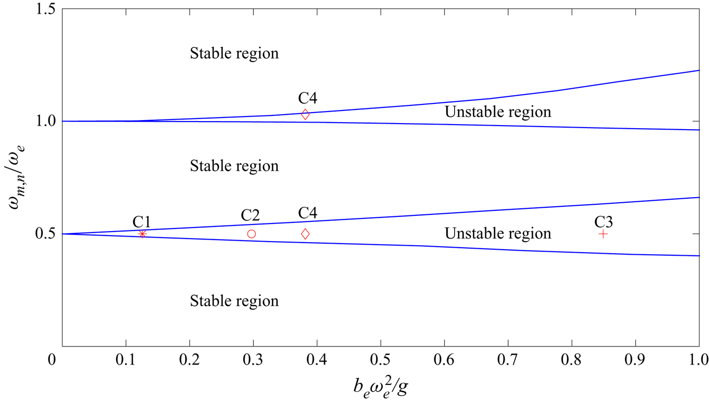
 ${b_e\omega _e^2}/g$ (McLachlan Reference McLachlan1947; Abramowitz & Stegun Reference Abramowitz and Stegun1965), and the contour plot of each natural frequency (Frandsen Reference Frandsen2004; Kumar & Tuckerman Reference Kumar and Tuckerman1994) is displayed in figure 2. It should be noted that after the normalisation of both axes, the contour plots for both free surface and interface instabilities are the same.

Based on figure 2, we determined four cases of frequency and amplitude combination to be investigated in this study. Case 1 (C1:  $m=1$,
 $n=2$) and case 2 (C2:
 $m=2$,
 $n=2$) correspond to Faraday wave of first mode and second mode on the free surface under subharmonic excitations (i.e.
 ${\omega _{m,n}}/{\omega _e}=0.5$). They will be studied by both experiments and numerical simulations in § 4.1. Case 3 (C3:
 $m=5$,
 $n=1$) corresponds to fifth-order Faraday waves on the interface during which the strong secondary interface instability in the RT instability type will occur and be investigated in § 4.2. Case 4 (C4:
 $m=1$,
 $n=2$ for free surface and
 $m=3$,
 $n=1$ for interface) corresponds to the first-order Faraday wave on free surface (harmonic, i.e.
 ${\omega _{m,n}}/{\omega _e}=1.0$) and third-order Faraday wave (subharmonic) on interface under the same external excitation, during which the secondary interface instability of KH type will take place and be investigated in § 4.3.
3. Experimental set-up
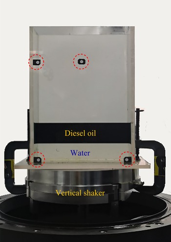
A series of experiments were conducted by utilising the dynamic triaxial apparatus in State Key Laboratory of Hydraulic Engineering Simulation and Safety in Tianjin University, China. A rigid tank, which is 0.25 m in length, 0.10 m in width and 0.45 m in height, sits on the triaxial apparatus (figure 3). The height of the tank is high enough so that no liquid is spilled out of the tank under the experimental conditions. The vertical movement of the tank can be precisely controlled by the motor in triaxial apparatus. The lower layer liquid is water with a density of  $998.0\,\mathrm {kg}\,\mathrm {m}^{-3}$ and the upper one is diesel oil with a density of
 $826.0\,\mathrm {kg}\,\mathrm {m}^{-3}$. The diesel oil was dyed with dark green colour and a video of the movement of the free surface and interface between oil and water was recorded. Standard image processing was used to track the movement of the free surface and interface simultaneously. In the experiment, a high-speed CCD camera with 60 Hz and a spatial resolution of
 $1920\times 1080$ pixels, which was fixed on a tripod standing on the ground, was used to record the free surface and interface motion. However, it is unavoidable that the tank in the frame is visually tilted due to the relative motion between the tank and the camera. To rectify the errors of image distortion, four controlling points were fixed on front side of the tank (circled in red in figure 3) and were used during the image processing. Therefore, no intruding equipment such as wave gauges was utilised to measure free surface and interface between liquids.
Experimental set-up of two-layer liquids (water and dyed diesel oil) with free surface under vertical excitation by using triaxial apparatus; four controlling points (red circles) are fixed on front side of the tank and used to rectify the errors of image distortion during image processing.

In the experiment, the depth of both layers  $h_1 = h_2 = 0.05$ m. Based on (2.11), the first and second natural frequencies related to the upper layer are
 $\omega _{1,2} = 10.1480\,\mathrm {s}^{-1}$ and
 $\omega _{2,2} = 15.5817\,\mathrm {s}^{-1}$, respectively. The vertical tank movement follows the sinusoidal function, i.e.
 $w_e = -b_e\omega _e\cos \omega _et$, in which
 $b_e$ and
 $\omega _e$ are the amplitude and frequency of the external excitation.
4. Faraday waves and secondary interface instability
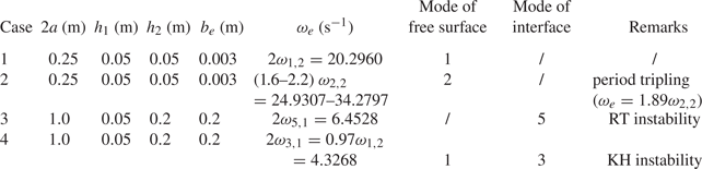
In the following text, we refer non-breaking Faraday waves to primary instability, whereas the breaking Faraday waves on free surface (e.g. period tripling breaking) as secondary surface instability, and the RT or KH instability that occurs on liquid interface as secondary interface instability. In this section, Faraday waves at both free surface and interface will be studied systematically, when the resonant response occurs on free surface, the interface between two liquids, and both simultaneously. Special attention will be paid to the secondary interface instabilities in the form of RT instability and KH instability when the interface Faraday wave is triggered. Although RT instability type of secondary interface instability is the result of combining external excitation and vertical fluid acceleration, which can take place even when the external excitation amplitude of acceleration is smaller than that of gravity, the KH type of secondary interface instability always takes place when both free surface and interface Faraday waves are excited with different modes and, thus, moving in different directions across the interface at certain instances. The parameters and the forms of secondary instability of the four cases to be presented in this section are listed in table 1.
Parameters of the study cases in § 4.

4.1. Faraday waves on free surface
In the first experiment, the frequency of external excitation  $\omega _e$ was set to be twice the first modal natural frequency related to the upper layer, i.e.
 $\omega _e = 2\omega _{1,2}=20.2960\, \mathrm {s}^{-1}$, and thus it was expected that the first mode resonant response of upper layer would occur. The amplitude of external excitation is
 $b_e = 0.003$ m (C1 in figure 2). In the numerical simulation, the length of the computational domain is 0.25 m and the height of the domain is 0.225 m. The employed mesh system has 200 uniform horizontal and 180 uniform vertical grid points with mesh size
 $\Delta x=\Delta z=0.00125$ m. The simulation runs up to
 $t\omega _{1,2}/(2{\rm \pi} ) = 64$ and the time step is automatically adjusted to ensure the stability of the numerical model. In order to trigger Faraday waves, the initial slopes of the free surface and the interfaces are set to
 $-10^{-5}$. In the experiment, on the other hand, the vertical vibration of the shaking table always contained background noise that was enough to trigger Faraday waves. A time shift of the numerical results was carried out to match the starting point of Faraday waves in experiment.
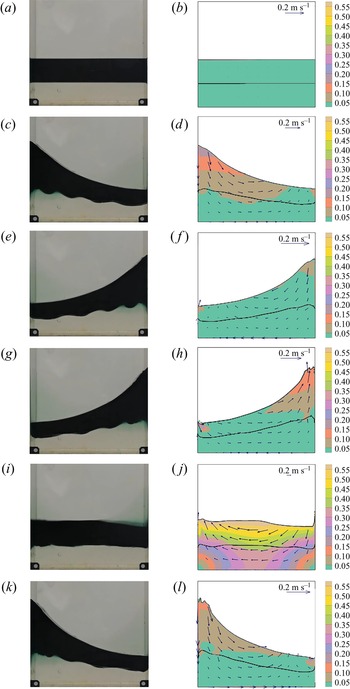
The comparisons of the snapshots of free surface and interface profiles from experiment and numerical simulation at  $t\omega _{1,2}/(2{\rm \pi} )$ = 16.0, 43.61, 44.11, 46.14, 46.40 and 46.64 are shown in figure 4, in which we can observe that the elevation of free surfaces becomes increasingly large and resonance occurs in two-layer Faraday waves. In addition, the numerical results of both free surface and interface profiles match favorably with those from experiment (left column), indicating that the hydrodynamic characteristics of layered Faraday waves can be well reproduced and predicted by NEWTANK. Both experiment and numerical simulation indicate that the interface moves in-phase along with the free surface, and the response of the lower layer liquid is basically a forced motion by the upper layer liquid. The numerical results of free surface and interface displacements at the position of
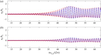
 $x = 0.115$ m (near the right boundary in figure 1) are also compared with the experimental data. It can be seen from figures 5(a) and 5(b) that fairly good agreements are obtained for both free surface and interface between the numerical results and experimental data. From figures 5(a) and 5(b) we can also observe that before
 $t\omega _{1,2}/(2{\rm \pi} ) = 20$, the responses of both free surface and interface are very small. However, after
 $t\omega _{1,2}/(2{\rm \pi} ) = 20$, resonant response gradually develops and the normalised free surface displacement is as large as 2 at
 $t\omega _{1,2}/(2{\rm \pi} ) = 46.7$. It should also be noted that the wave crest becomes sharper and the trough becomes flatter after
 $t\omega _{1,2}/(2{\rm \pi} ) = 40.0$, indicating that nonlinearity begins to take effect. Furthermore, after
 $t\omega _{1,2}/(2{\rm \pi} ) = 40.0$, the effect of nonlinearity restricts the wave amplitude to unboundedly grow. Instead, the response begins to become smaller. Actually, as the wave height increases due to resonant effect, wave nonlinearity becomes strong. As a result, the wave celerity exceeds that of linear wave, based on which the natural frequencies of the liquid system are calculated and the external excitation is selected. The difference of the external excitation frequency and the actual natural frequency of the liquid system will become larger and larger until the surface breaks up or the resonance stops when the frequency difference is large enough.
Comparisons of snapshots of Faraday waves on the free surface and the interface under vertical excitation with  $b_e = 0.003$ m and
 $\omega _e = 2.0\omega _{1,2}$ at
 ${t \omega _{1,2}}/{2{\rm \pi} } = 16.0$, 43.61, 44.11, 46.14, 46.40 and 46.64 between the experimental results (a,c,e,g,i,k) and the numerical results (b,d,f,h,j,l); the colour in the right column indicates the velocity magnitude and the vectors are the velocity field; the black lines indicate the profiles of the free surface and the interface between two liquids.

Comparisons of normalised displacement of (a) free surface and (b) interface at  $x = 0.115$ m in a vertically excited tank with
 $b_e = 0.003$ m and
 $\omega _e = 2.0\omega _{1,2}$ between the numerical results (solid line) and the experimental data (circles).

Observation is made to the small waves on the interface in experiment (figures 4c, 4e and 4g), which are not well-captured in the numerical simulation. When we conducted stability analysis, it is found that these small waves may arise from the higher-mode response of the interface Faraday waves. The natural frequency of the 9th mode of the lower layer is  $\omega _{9,1}=10.2284\,\textrm {s}^{-1}$, which is rather close to
 $\omega _{1,2}=10.1480\,\textrm {s}^{-1}$. This can be confirmed from figures 4(c), 4(e) and 4(g) that the interface contains 4.5 waves. However, due to the fact that the disturbances to trigger these interface Faraday waves in experiment cannot be exactly reproduced in the numerical simulation, the small interface waves in the numerical modelling appear much later and do not match the laboratory observations in the same pace, even though the numerical simulations capture some of the larger oscillations near the walls, where the interface Faraday waves are first triggered.
In the second experiment, the frequency of external excitation  $\omega _e$ was set to be twice the second mode natural frequency related to the upper layer, i.e.
 $\omega _e = 2\omega _{2,2} = 31.1742\,\mathrm {s}^{-1}$, in which the second mode resonant response of upper layer may occur (C2 in figure 2). The same amplitude of external excitation was adopted as in previous set-up. In the computation, the length of the computational domain is 0.25 m, and the height of the domain is 0.2 m. The employed mesh system has 200 uniform horizontal and 160 uniform vertical grids with mesh size
 $\Delta x=\Delta z=0.00125$ m. The simulation runs up to
 $t \omega _{2,2}/ (2{\rm \pi} ) = 47$ and the time step is automatically adjusted to ensure the stability of the numerical model. The same initial slope of free surface and interface is adopted as in previous case. In this laboratory experiment, the acceleration amplitude of the vertical excitation has already reached the limit of the apparatus, and thus the experiment stopped before
 $t \omega _{2,2}/ (2{\rm \pi} ) = 45$ for device protection.
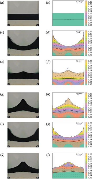
The comparisons of the snapshots of free surface and interface profiles from experiment and numerical simulation at  $t\omega _{2,2}/(2{\rm \pi} )$ = 14.88, 28.94, 29.21, 29.43, 30.06 and 31.54 are shown in figure 6, in which symmetric wave profiles of the 2nd mode resonance can be seen. Again, the numerical results of both free surface and interface profiles match well with those from experiment. The numerical results of free surface and interface displacement at the center of the tank (
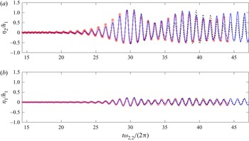
 $x=0$ in figure 1) are compared with the experimental data. It can be seen from figures 7(a) and 7(b) that fairly good agreements are obtained for both free surface and interface between the numerical results and experimental data. From figures 7(a) and 7(b) we can also observe that before
 $t\omega _{2,2}/(2{\rm \pi} ) = 20.0$, the responses of both free surface and interface are very small. After
 $t\omega _{2,2}/(2{\rm \pi} ) = 20.0$, resonant response gradually develops and the free surface displacement normalised by the depth of the lower layer liquid is as large as 1.2 at
 $t\omega _{2,2}/(2{\rm \pi} ) = 29.5$. It should also be noted that the wave crest becomes sharper and the trough becomes flatter after
 $t\omega _{2,2}/(2{\rm \pi} ) = 25$, similar to that observed in case 1. Furthermore, after
 $t\omega _{2,2}/(2{\rm \pi} ) = 29.5$, the wave amplitude gradually decreases due to frequency shift. The similar small interface Faraday waves are also observed in experiment for this case as those in previous experiment, except that this time they are of the 21st mode, i.e.
 $\omega _{21,1}=15.6243,\textrm {s}^{-1}$, which is close to
 $\omega _{2,2}=15.5817\,\textrm {s}^{-1}$.
Comparisons of snapshots of Faraday waves on the free surface and the interface under vertical excitation with  $b_e = 0.003$ m and
 $\omega _e = 2.0\omega _{2,2}$ at
 ${t \omega _{2,2}}/{2{\rm \pi} }$ = 14.88, 28.94, 29.21, 29.43, 30.06 and 31.54 between the experimental results (a,c,e,g,i,k) and the numerical results (b,d,f,h,j,l); the colour in the right column indicates the velocity magnitude and the vectors are the velocity field; the black lines indicate the profiles of the free surface and the interface between two liquids.

Comparisons of normalised displacement of (a) free surface and (b) interface at  $x = 0$ in a vertically excited tank with
 $b_e = 0.003$ m and
 $\omega _e = 2.0\omega _{2,2}$ from the experimental data (circles), the numerical results with turbulence model (blue solid line) and numerical results without turbulence model (black dashed line).

The turbulence effect is examined by turning off the turbulence model and re-run the same case. The numerical results without turbulence model is added into figure 7. It can be seen from figure 7(a) that before  $t\omega _{2,2}/(2{\rm \pi} ) = 32$, the differences of all results are negligible; however, the numerical results without turbulence model deviate from the experimental data gradually after
 $t\omega _{2,2}/(2{\rm \pi} ) = 32$, whereas the numerical results with LES model match well with the experimental data, indicating that the turbulence model plays a crucial role in long-term simulation when the wave amplitude becomes large.
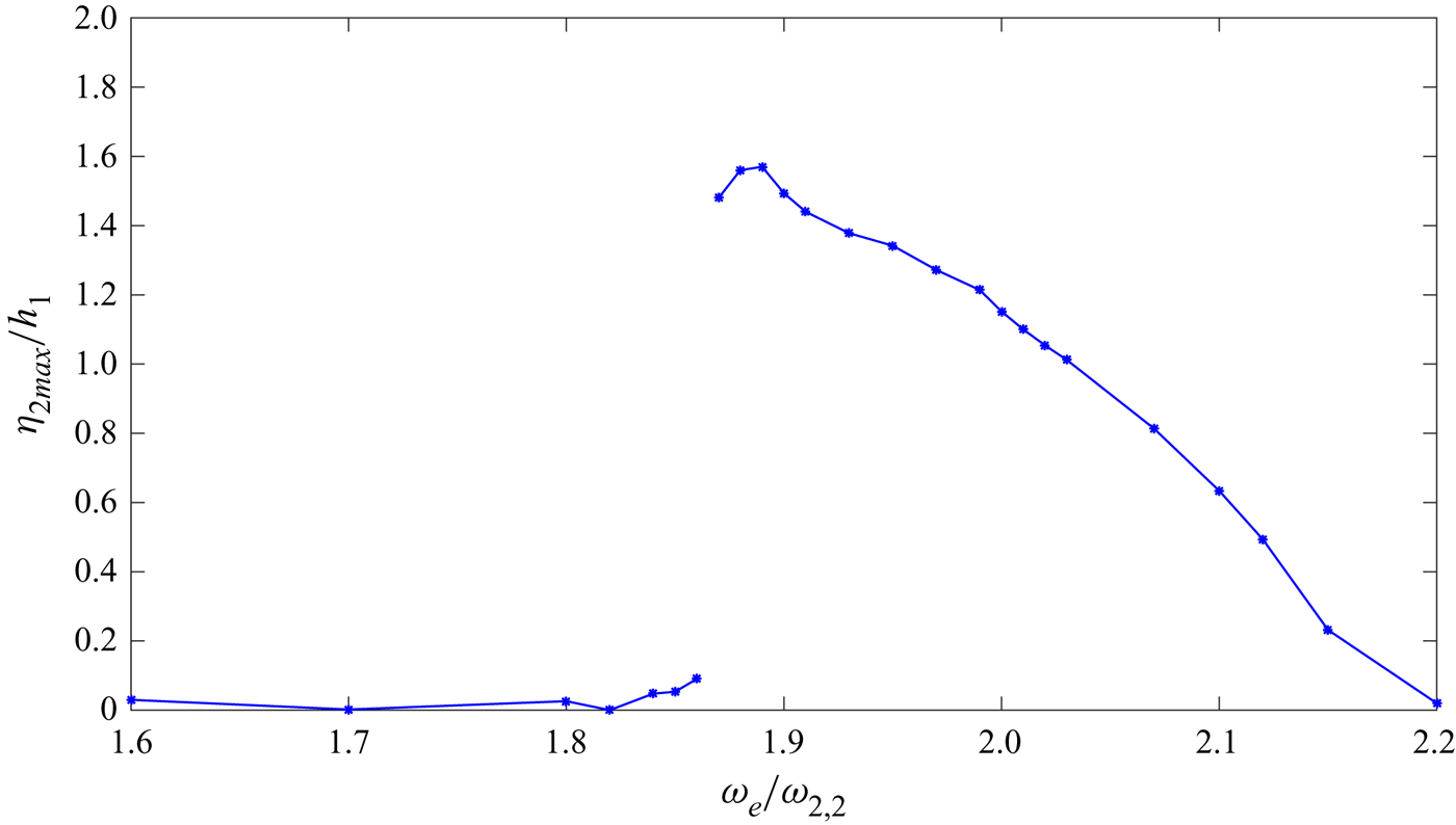
In order to investigate the off-resonant, near-resonant and resonant responses, we extend case 2 for more external excitations with the ratio of  $\omega _e/\omega _{2,2}$ varying from
 $1.6$ to
 $2.2$. The change of free surface Faraday wave amplitude with excitation frequency is shown in figure 8. When
 $\omega _e / \omega _{2,2} \le 1.86$, the maximum free surface displacement (
 $\eta _{2{max}}$) of Faraday waves are relatively small; however, when
 $\omega _e/\omega _{2,2} = 1.87$, the maximum displacement of Faraday waves normalised by the depth of the lower layer liquid rises sharply to 1.48. The maximum displacement occurs when
 $\omega _e / \omega _{2,2} = 1.89$ with
 $\eta _{2{max}}/h_1$ being 1.57. When
 $\omega _e/\omega _{2,2} > 1.89$, the response of Faraday waves decreased gradually until
 $\eta _{2{max}}/h_1 = 0.02$ when
 $\omega _e /\omega _{2,2} = 2.2$. It should be noted that the maximum response of Faraday waves on the free surface occurs when
 $\omega _e /\omega _{2,2} = 1.89$, instead of 2.0. When the maximum response of the Faraday waves on the free surface occurs at
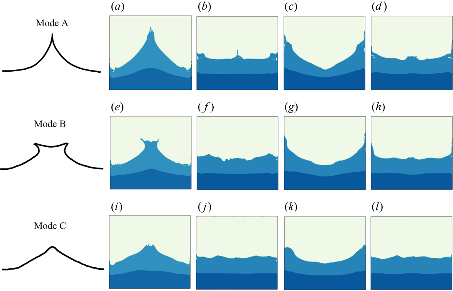
 $\omega _e /\omega _{2,2} = 1.89$, it can be seen from figure 9 that the phenomenon similar to the period tripling breaking modes proposed in Jiang, Perlin & Schultz (Reference Jiang, Perlin and Schultz1998) can also be found in the two-layer liquids with free surface. When the response of Faraday waves is large, the breaking waves, which can be regarded the secondary surface instability, are in the form of three modes at three successive periods, i.e. sharp crest (mode A), dimpled or flat crest with plunging breaker on both sides (mode B) and round crest (mode C). When the resonant waves are generated on the free surface and the response becomes maximum in the middle of the tank at
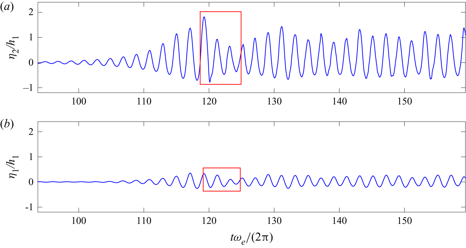
 $t\omega _e/(2{\rm \pi} ) = 119.24$, as can be seen from figure 10, the profile of the free surface is similar to the shape of mode A, and in the following two periods, the profiles of the free surface resemble the shape of mode B and mode C introduced by Jiang et al. (Reference Jiang, Perlin and Schultz1998).
Normalised responses of free surface displacement when  $\omega _e / \omega _{2,2}$ ranges from 1.6 to 2.2.

Snapshots of breaking Faraday waves on free surface under vertical excitations of  $b_e = 0.003$ m and
 $\omega _e = 1.89\omega _{2,2}$ in three successive periods: (a) occurs at
 ${t \omega _e}/{2{\rm \pi} } = 119.24$ and the time interval between each two parts (a)–(l) is
 ${1}/{4}$ period of response (
 $T_r = {2{\rm \pi} }/{\omega _r} = 0.4267$ s).

Normalised displacements of (a) the free surface and (b) the interface at  $x = 0$ in a vertically excited tank with
 $b_e = 0.003$ m and
 $\omega _e = 1.89\omega _{2,2}$; the red rectangle indicates the time interval when period tripling on the free surface can be observed.

Scale effects are investigated in this study. Due to the limitation of our experimental apparatus, we only conducted experiments using a small tank (described in § 3), which was 0.25 m in length ( $l_e$), 0.10 m in width and 0.45 m in height. The scale effects were investigated numerically by running additional simulations of different scale problems with similar tank geometry. The tanks utilised in these simulations were of the dimension with the length
 $\times$ width equal to 1.0 m
 $\times$ 0.4 m (tank 1,
 $l_1$), 5.0 m
 $\times$ 2.0 m (tank 2,
 $l_2$) and 25.0 m
 $\times$ 10.0 m (tank 3,
 $l_3$). Therefore, the ratios of length scale
 $\lambda _i=l_i/l_e$ for the four tanks were 1, 4, 20 and 100, respectively. As the inertial force and gravitational force were the dominant forces in Faraday waves, the Froude number (
 $Fr$) similarity was required so that
 $V_e/\sqrt {gl_e} =V_i/\sqrt {gl_i}$, where
 $i = 1,2,3$. Therefore, the time scale
 $T_i/T_e = \sqrt {l_i/l_e} = \sqrt {\lambda _i}$, which gave
 $T_e:T_1:T_2:T_3 = 1:2:2\sqrt {5}:10$. In the simulations, we used the same viscosity and, thus, the Reynolds number (
 $Re$) increased with the size of the tank.
By using (2.10) and (2.11), it was found that the second mode natural frequencies of three additional numerical models are 7.79, 3.48 and 1.56 s $^{-1}$, which could be calculated by
 $Fr$-based similarity law as well. Case 2 with
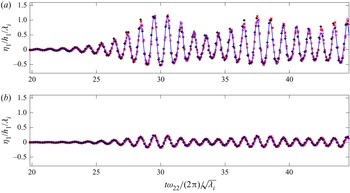
 $\omega _e/\omega _{2,2} = 2.0$ was again utilised to analyse the scale effects. It was seen from figure 11 that four results (normalised by the respective time and length scale) were rather close, implying that for non-breaking Faraday waves, the
 $Fr$ similarity was adequate to describe scale effects, i.e. the wave height increased linearly in a larger tank if the excitation is scaled linearly. The small discrepancies among numerical results of different length scales probably arose from the viscous effect, which was not the dominant factor for non-breaking waves.
Comparisons of normalised displacement of (a) free surface and (b) interface at  $x = 0$ in a vertically excited tank with
 $\omega _e = 2.0\omega _{2,2}$ from the numerical results of experimental scale (blue solid line), length scale 1 (red crosses), length scale 2 (magenta circles) and length scale 3 (black pluses).

4.2. Faraday waves on interface and secondary interface instability
In § 4.2, the Faraday waves at the interface between liquids will be studied. As the interface Faraday wave grows, the combined effects of external excitation and fluid acceleration in vertical direction may exceed the threshold of gravity and induce the secondary instability in the form of RT instability, which becomes 3-D eventually.
To capture the possible 3-D flow evolution during the secondary instability, a larger tank than that utilised in the experiment with the length of  $2a = 1.0$ m, the width of
 $2w = 0.15$ m, the height of
 $H = 0.3$ m is adopted in the numerical simulation. The depth of the lower layer is
 $h_1 = 0.05$ m and the depth of the upper layer is
 $h_2 = 0.20$ m, with the density of the lower layer being
 $\rho _1 = 1.0 \times 10^3\,\mathrm {kg}\,\mathrm {m}^{-3}$ and the density of the upper layer
 $\rho _2 = 0.84 \rho _1$. Therefore, with
 $g = 9.81\,\mathrm {m}\,\mathrm {s}^{-2}$, the fifth mode of natural frequency related to lower layer response
 $\omega _{5,1} =3.2264\,\mathrm {s}^{-1}$. As the initial disturbance, the interface between liquids in the tank is set as a straight line with the slope of
 $s = 0.01$. In the simulation, the frequency of external excitation is
 $\omega _e = 2\omega _{5,1} = 6.4528\,\mathrm {s}^{-1}$, and the amplitude is
 $b_e = 0.2$ m. Thus, the period of vertical excitation
 $T_e = 0.5 T_{5,1}$. The oscillation of the tank follows
 ${\mathrm {d}w_e}/{\mathrm {d}t} = b_e\omega _e^2\sin (\omega _et)$. Therefore, the acceleration amplitude of vertical external excitation is
 $b_e\omega _e^2 = 8.3277\,\mathrm {m}\,\mathrm {s}^{-2}$, which is approximately
 $0.85g$.
When the motion of the free surface is negligible and only the Faraday waves on the interface are significant, as shown in figure 12, the linear stability map of the interface between two fluids is similar to the original one of Benjamin & Ursell (Reference Benjamin and Ursell1954), according to Kumar & Tuckerman (Reference Kumar and Tuckerman1994). The subharmonic case considered here is displayed in figure 2 (C3). With such a set-up, the fifth order of interface Faraday wave is expected to be induced, whereas the free surface is off resonance. In the numerical simulation, the horizontal grids have a mesh size  $\Delta x=\Delta y=0.005$ m and the vertical grids
 $\Delta z=0.0015$ m. The time step is automatically adjusted to ensure the numerical stability. The simulation runs up to
 $t = 15$ s.
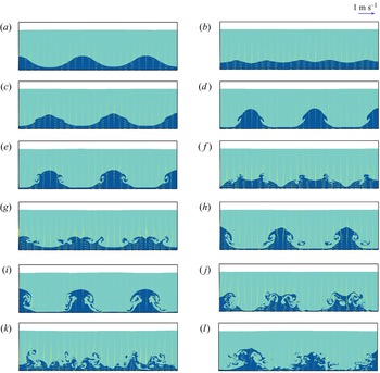
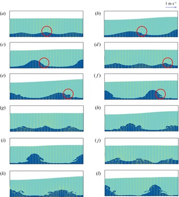
Snapshots of Faraday waves on the free surface and the interface under vertical excitation with  $b = 0.2$ m and
 $\omega _e =2\omega _{5,1}$ at (a)
 $t= t_0+T_{5,1}/8$, (b)
 $t= t_0+T_{5,1}/4$,(c)
 $t= t_0+3T_{5,1}/8$, (d)
 $t= t_0+T_{5,1}/2$, (e)
 $t= t_0+5T_{5,1}/8$, (f)
 $t= t_0+3T_{5,1}/4$, (g)
 $t= t_0+7T_{5,1}/8$, (h)
 $t= t_0+T_{5,1}$, (i)
 $t= t_0+9T_{5,1}/8$, (j)
 $t= t_0+5T_{5,1}/4$, (k)
 $t= t_0+11T_{5,1}/8$ and (l)
 $t= t_0+13T_{5,1}/8$.

The snapshots of the free surface and interface at the mid-plane of the tank width at  $t= t_0+T_{5,1}/8$,
 $t_0+T_{5,1}/4$,
 $t_0+3T_{5,1}/8$,
 $t_0+T_{5,1}/2$,
 $t_0+5T_{5,1}/8$,
 $t_0+3T_{5,1}/4$,
 $t_0+7T_{5,1}/8$,
 $t_0+T_{5,1}$,
 $t_0+9T_{5,1}/8$,
 $t_0+5T_{5,1}/4$,
 $t_0+11T_{5,1}/8$ and
 $t_0+13T_{5,1}/8$ are shown in figure 12 (
 $t_0=9T_e$). It can be found that the displacement of the interface is much larger than that of the free surface, as expected. In addition, the Faraday waves in the interface become increasingly high as time evolves. At
 $t = t_0+T_{5,1}/8$, the fifth mode response on interface with two waves and a half can be seen in figure 12(a). These Faraday waves start to break at
 $t = t_0+3T_{5,1}/8$ (figure 12c), due to the nonlinear effect in the interface Faraday waves with increasing wave amplitude. At
 $t = t_0+T_{5,1}/2$ (figure 12d), an interesting phenomenon can be observed that the wave crests are of ‘mushroom-hat’ style. As the wave crests become even higher, secondary interface instability is formed at
 $t = t_0+7T_{5,1}/8$ and
 $t = t_0+T_{5,1}$ (figures 12g and 12h). As the development of wave trough in the interface is restricted by the bottom of the tank, almost all the liquids in the lower layer form the crest of RT mushroom-hat and the wave trough becomes very thin, and the nonlinearity becomes much stronger. Afterwards, the flow becomes chaotic as can be seen from figures 12(i)–12(l).
It is found that the shape of unstable interface is very similar to RT instability that occurs when a heavier liquid enters the lighter liquid from above under gravity. Once the heavier liquid on the top layer begins to moves downward, the liquid on the lower layer will move upward to fill the space left by the heavier liquid. As the liquid on lower layer cannot provide enough buoyancy for heavier liquid, the initial disturbance will be magnified, leading to instability. This can also happen on the interface of two liquids when the heavier liquid is below the lighter one, but the imposed vertical excitation exceeds the gravitational acceleration (Waddell, Niederhaus & Jacobs Reference Waddell, Niederhaus and Jacobs2001). This creates time intervals during which the upper liquid becomes essentially heavier than the lower one (Cerda & Tirapegui Reference Cerda and Tirapegui1997, Reference Cerda and Tirapegui1998; Lioubashevski et al. Reference Lioubashevski, Fineberg and Tuckerman1997).
However, our case is different from either of these two situations. We have the lighter liquid in the upper layer and the maximum acceleration amplitude of the vertical excitation remains lower than that of gravity. From the viewpoint of statics, this system is stable. However, after carefully inspecting how this secondary instability is initiated and evolved, we realise that there is an additional factor that plays an important role that has not been adequately considered in the previous studies. This factor is fluid particle acceleration in Faraday waves and it will modify the stability criterion of the dynamic two-liquid system, especially when the wave amplitude grows beyond certain threshold. In other words, the RT instability in this case actually results from large-amplitude Faraday waves on the interface between two liquids, and thus we refer to it as secondary interface instability, in contrast to the primary instability of Faraday wave itself. In order to quantify the fluid acceleration contribution, we introduce a new parameter for a dynamic fluid system. The detailed derivation is given in the following.
From (2.2), we can have the NSE for the vertical direction with the positive direction pointing upward, i.e.
 $$\begin{gather} \frac{\partial w}{\partial t}+u\frac{\partial w}{\partial x}+v\frac{\partial w}{\partial y}+w\frac{\partial w}{\partial z} ={-}\frac{1}{\rho} \frac{\partial p}{\partial z}+\frac{1}{\rho} \frac{\partial \left( \tau_{zx}+R_{zx} \right)} {\partial x} + \frac{1}{\rho}\frac{\partial \left( \tau_{zy}+R_{zy} \right)}{\partial y}\nonumber\\ +\frac{1}{\rho} \frac{\partial \left( \tau_{zz}+R_{zz} \right)}{\partial z} + g_z - \frac{\mathrm{d}w_e}{\mathrm{d}t}, \end{gather}$$
Rearranging the equation with all of the acceleration terms on the left-hand side and setting  $g_z=-g$, we have:
 $$\begin{gather} g+\left( \frac{{\rm d}w_e}{{\rm d}t}+\frac{\partial w}{\partial t}+{u}\frac{\partial w}{\partial x}+{v}\frac{\partial w}{\partial y}+{w}\frac{\partial w}{\partial z}\right) ={-}\frac{1}{\rho} \frac{\partial p}{\partial z}+\frac{1}{\rho} \frac{\partial \left( \tau_{zx}+R_{zx} \right)} {\partial x} \nonumber\\ +\frac{1}{\rho}\frac{\partial \left( \tau_{zy}+R_{zy} \right)}{\partial y} +\frac{1}{\rho} \frac{\partial \left( \tau_{zz}+R_{zz} \right)}{\partial z}. \end{gather}$$
We call the left-hand side the effective gravitational acceleration. If we normalise it with  $g$, then a dimensionless parameter normalised effective gravitational acceleration (NEGA) is obtained, i.e.
 \begin{equation} \mathrm{NEGA} = 1+\left(\frac{{\rm d}w_e}{{\rm d}t}+\frac{\partial w}{\partial t}+{u}\frac{\partial w}{\partial x}+{v}\frac{\partial w}{\partial y}+{w}\frac{\partial w}{\partial z}\right)/g. \end{equation}
NEGA accounts for the gravity together with vertical excitation and fluid acceleration. When NEGA  $>0$, the fluid system is stable, whereas when NEGA
 $\leq 0$, RT instability may occur locally.
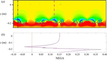
If the spatial distribution of NEGA at  $t = t_0+7T_{5,1}/8$, which corresponds to figure 12(g), is calculated and plotted in figure 13(a), we can spot a few regions (with blue colour) where NEGA
 $<0$, implying that the secondary instability in the form of RT instability will be induced in the near future (figure 12h). The distribution of NEGA at
 $t_0+7T_{5,1}/8$ can be seen from figure 13(a), whereas the vertical distributions of NEGA at
 $x = -0.4425$ and
 $-0.0575$ are plotted in figure 13(b). As can be seen from figure 13, at
 $t = t_0+7T_{5,1}/8$, there is a turning point for NEGA near the interface, and the values of NEGA here are indeed smaller than zero. Thus, the conditions of RT instability are satisfied locally. As a result, after another
 $T_{5,1}/8$ at
 $t = t_0+T_{5,1}$, it can be seen from figure 12(h) that mushroom-hat shaped secondary instability resembling the shape of classic RT instability (Waddell et al. Reference Waddell, Niederhaus and Jacobs2001) is generated on the interface. From figure 13, we can find the possible locations that secondary instabilities may occur. The NEGA at the location of
 $(-0.4425,-0.16375)$ m is utilised to investigate the contribution of the gravity, the periodic vertical excitation, the local acceleration and the convective acceleration to NEGA. It can be seen from figure 14 that at the location of
 $(-0.4425,-0.16375)$ m the value of NEGA is smaller than
 $0$ at
 $t = t_0+7T_e/4 = 10.75T_e$, which is why the liquid here at this moment can generate secondary RT instability, even though the time duration for NEGA
 $<0$ is short and the total area of unstable flow regions is small.
(a) The spatial distribution of the normalised effective gravitational acceleration (NEGA) in Faraday waves under vertical oscillations with  $b_e$ = 0.2 m and
 $\omega _e = 2\omega _{5,1}$ at
 $t = t_0+7T_{5,1}/8$; the grey line indicates the profile of the interface between two liquids; (b) the corresponding vertical variation of NEGA at
 $x = -0.4425$ m (black dash-dot line) and
 $-0.0575$ m (magenta dashed line).

Time series of NEGA (black solid line), gravitational acceleration (red dotted line), acceleration of vertical excitation (blue dashed line), local acceleration (circles) and convective acceleration (cross) at the position of  $(x,z) = (-0.4425,-0.16375)$ m. The green circle denotes the time interval when
 $\mathrm {NEGA} < 0$, which is also around the moment in figure 13, i.e.
 $t = t_0+7T_{5,1}/8 = 10.75T_e$.

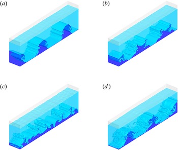
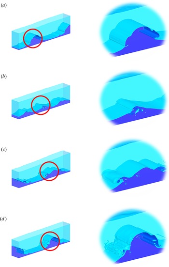
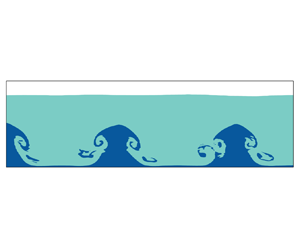
When secondary RT instability is generated, the flow structure has a tendency to transform from 2-D to 3-D. As can be seen from figure 15, after the secondary RT instability occurs at  $t = t_0+T_{5,1}$, symmetric vortices generated on both sides of the Faraday waves (figure 12h) enhance the mixture of two liquids (figure 15a) and the liquids of both layers near the interface further mix together at
 $t = t_0+5T_{5,1}/4$ (figure 15b). Then the interface can no longer sustain the 2-D structure and breaks down (figure 15c), and finally evolves into 3-D flow structure at
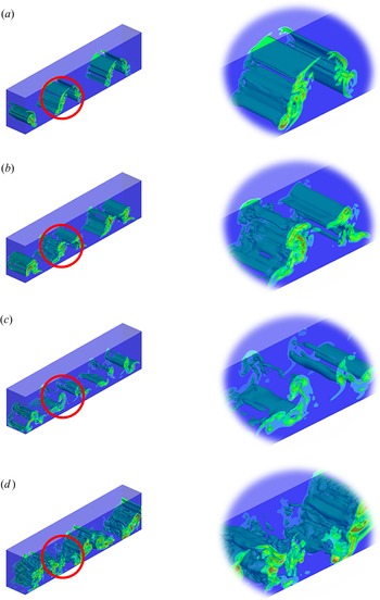
 $t = t_0+13T_{5,1}/8$ in figure 15(d). The corresponding vorticity near the interface between two liquids is plotted in figure 16. It can be seen that at
 $t = t_0+T_{5,1}$ when the interface just breaks due to strong nonlinear effect, the vortex tube is still nearly 2-D. However, as time evolves, the vortex structures become more and more 3-D, caused by the secondary interface instability of RT type.
Snapshots of 3-D Faraday waves on the free surface and the interface under vertical excitation with  $b_e = 0.2$ m and
 $\omega _e = 2\omega _{5,1}$ at (a)
 $t= t_0+9T_{5,1}/8$, (b)
 $t= t_0+5T_{5,1}/4$, (c)
 $t= t_0+11T_{5,1}/8$ and (d)
 $t= t_0+13T_{5,1}/8$, which correspond to figures 12(i)–12(l).

Snapshots of 3-D vorticity field near the interface between two liquids under vertical excitation with  $b_e = 0.2$ m and
 $\omega _e =2\omega _{5,1}$ at (a)
 $t= t_0+9T_{5,1}/8$, (b)
 $t= t_0+5T_{5,1}/4$, (c)
 $t= t_0+11T_{5,1}/8$ and (d)
 $t= t_0+13T_{5,1}/8$, which correspond to figures 12(i)–12(l).

To further understand the particle behaviour in this secondary instability, the trajectory of a massless particle originally located at  $(-0.3,0,-0.205)$, i.e.
 $2a/5$ away from the left wall and
 $h_1/10$ below the original interface, is plotted in figure 17 for 14 periods of vertical oscillation. The trajectory for the first 8 periods is coloured blue, the 9th and 10th periods cyan, the 11th and 12th green and the last 2 periods red. It can be seen from figure 17(a) that during the first 8 periods, the movement of the particle is restricted within a very thin region, implying that the motion is essentially 2-D. As the interface Faraday waves grows under resonant excitation, the range of movement of the trajectory becomes larger, yet it is still confined within the 2-D mid-plane of tank until 12th period, as shown in figure 17(b). However, after that, the trajectory of the particle moves out of the mid-plane and become total 3-D under RT instability.
(a) 3-D view and (b) side view of the trajectory of a particle originally located at  $(-0.3,0,-0.205)$ in 14 periods of vertical oscillation; the 1st–8th periods in blue, the 9th and 10th periods in cyan, 11th and 12th periods in green and 13th and 14th periods in red.

It should be noted that after interface instability occurs, turbulence becomes much stronger and many liquid droplets are formed near the interface where surface tension plays an important role. As we do not have experimental data at this moment, the accuracy of the numerical results in the stage of post-RT instability has not been validated and, thus, they mainly serve as the demonstration to provide qualitative analysis and discussion.
4.3. Faraday waves on both free surface and interface
In § 4.3, the two-layer Faraday waves with the frequency of vertical excitation equal to twice the natural frequency related to lower layer and simultaneously near the natural frequency related to upper layer are studied. As the resonant response of Faraday waves at the free surface and interface have different modes, reverse flows across the interface lead to KH instability as the flow directions of the upper wave and the lower wave are opposite.
In the following simulation, the length of the 3-D tank  $2a = 1.0$ m, the width
 $2w = 0.15$ m, in which the same liquids with the same depth as those in § 4.2 are adopted. Therefore, with
 $g = 9.81\,\mathrm {m}\,\mathrm {s}^{-2}$, the third mode of natural frequency related to lower layer response
 $\omega _{3,1} = 2.1634\,\mathrm {s}^{-1}$, and the first mode of natural frequency related to upper layer response
 $\omega _{1,2} = 4.4557\,\mathrm {s}^{-1}$.
Initially, both the free surface and the interface between liquids in the tank are straight lines with the same slope of  $s = 0.01$. The frequency of external excitation
 $\omega _e = 2\omega _{3,1} = 0.97\omega _{1,2} = 4.3268\,\mathrm {s}^{-1}$, and the amplitude
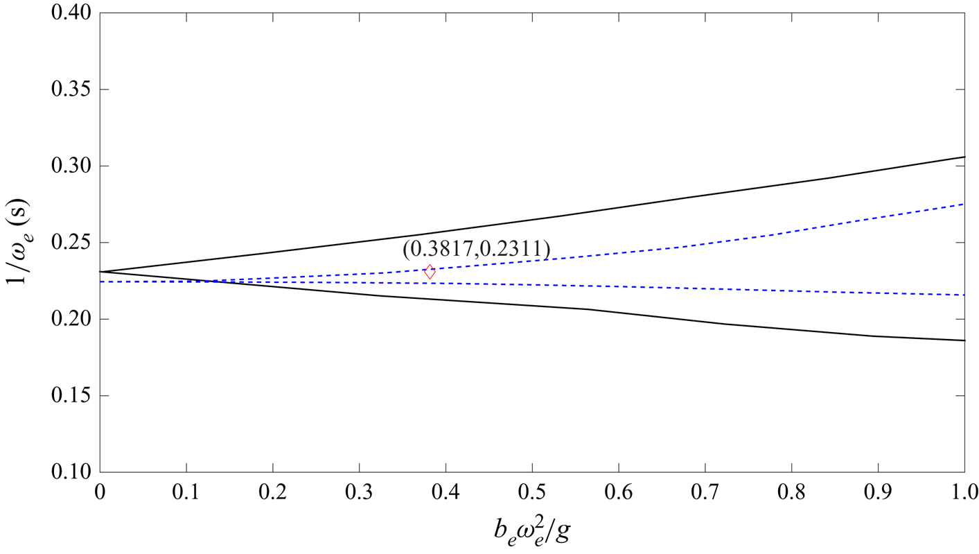
 $b_e = 0.2$ m. If we plot both the subharmonic and harmonic instability region under the same frequency of vertical excitation, as shown in figure 18, it can be found that there exists an overlapping area, in which the vertical oscillation of the tank can generate both subharmonic instability at the interface and harmonic instability at the free surface. Therefore, it is expected that the interface will have the third mode response and the free surface the first mode (C4 in figure 2). The mesh system has uniform horizontal grids with
 $\Delta x=\Delta y=0.005$ m and uniform vertical grids with
 $\Delta z=0.0015$ m. The time step is automatically adjusted to ensure the numerical stability. The simulation runs up to
 $t = 50$ s.
Instability diagram for Faraday waves when  $\omega _e = 2\omega _{3,1} = 0.97\omega _{1,2}$ and both the free surface and the interface exhibit resonance under the same vertical oscillation; black solid lines indicate the subharmonic instability region for the interface Faraday waves, blue dashed lines indicate the harmonic instability region for the free surface and red diamond is the test condition of vertical excitation.

The snapshots of the free surface and interface at the mid-plane of the tank width at  $t = t_0+3T_{3,1}/4$,
 $t_0+7T_{3,1}/8$,
 $t_0+T_{3,1}$,
 $t_0+5T_{3,1}/4$,
 $t_0+11T_{3,1}/8$,
 $t_0+3T_{3,1}/2$,
 $t_0+7T_{3,1}/4$,
 $t_0+15T_{3,1}/8$,
 $t_0+2T_{3,1}$,
 $t_0+9T_{3,1}/4$,
 $t_0+19T_{3,1}/8$ and
 $t_0+5T_{3,1}/2$ are shown in figure 19 (
 $t_0=16T_e$). It is found that both the free surface and interface are excited, but the modes of responses are different with the free surface being first mode and the interface third mode, because the frequency of excitation is equal to twice the third mode natural frequency of the lower layer and near the first mode natural frequency of the upper layer. Therefore, unlike the case in § 4.2, the velocity in upper layer liquid is also excited and move in one direction under first mode response. On the other hand, as the lower layer liquid has third mode response with shorter wavelength, the flow directions can be different at different locations, which provide chances of reverse flows across the interface driven by upper and lower layer liquids, respectively.
Snapshots of Faraday waves on the free surface and the interface under vertical excitation with  $b_e = 0.2$ m and
 $\omega _e = 2\omega _{3,1} = 0.97\omega _{1,2}$ at (a)
 $t= t_0+3T_{3,1}/4$, (b)
 $t= t_0+7T_{3,1}/8$, (c)
 $t= t_0+T_{3,1}$, (d)
 $t= t_0+5T_{3,1}/4$, (e)
 $t= t_0+11T_{3,1}/8$, (f)
 $t= t_0+3T_{3,1}/2$, (g)
 $t= t_0+7T_{3,1}/4$, (h)
 $t= t_0+15T_{3,1}/8$, (i)
 $t= t_0+2T_{3,1}$, (j)
 $t= t_0+9T_{3,1}/4$, (k)
 $t= t_0+19T_{3,1}/8$ and (l)
 $t= t_0+5T_{3,1}/2$.

Figure 19 exhibits how a KH instability is induced on the interface within two cycles, with figures 19(a)–19(f) representing the first cycle and figures 19(g)–19(l) the second cycle. At  $t = t_0+3T_{3,1}/4$, it can be seen from figure 19(a) that the flow direction of the upper layer liquid is mainly rightwards, whereas the flow direction of the lower layer liquid near the middle of the tank length is in opposite direction. It is seen from figure 19(b) that after another
 $T_{3,1}/8$ at
 $t = t_0+7T_{3,1}/8$, a vortex is formed in the wave front and there seems a tendency that this vortex will break if it further evolves. However, at
 $t = t_0+T_{3,1}$ in figure 19(c), the direction of the upper layer liquid changes to be leftward, which actually suppresses the vortex development and the interface becomes symmetric again. Nevertheless, the reverse flows occur in other places, i.e. the crest near the right wall in figure 19(d). This will further evolve into an overturning interface as shown in figures 19(e)–19(f). In each cycle, the interface will go through two phases of reserve flows and in-direction flows, respectively, with the former tending to develop into KH instability and the latter suppressing it.
However, as the Faraday waves grow on both the free surface and the interface, the phase of developing KH instability will win as shown in figures 19(g)–19(l), which is the second cycle that essentially repeat the processes as in figures 19(a)–19(f) but with larger amplitude of excited Faraday waves. Once the secondary interface instability is strong enough to evolve into a 3-D mode, it can no longer be suppressed by the in-direction flows of the second phase, as in figure 19(l).
It is worth pointing out that although the shape of interface instability in figure 19(l) looks similar to that in figure 12(e), the generating mechanisms are totally different. In § 4.2, the upper liquid is not in resonant mode and thus the free surface displacement is small at all time. The fluid velocity in the upper layer is always small except near the interface where the upper liquid must respond the excited interface motion. The vortices generated in the case of § 4.2 are mainly due to the fact that as the Faraday waves at the interface become strong, the secondary RT instability is generated, in which the space of the rising liquid from lower layer needs to be filled by the upper layer liquids, consequently generating vortices. In the present case, however, the motion of the upper liquid is more like the current in a U-tube with alternating directions. The vortices are induced mainly by the strong shear from the liquids of different layers moving at different directions at certain instances.
When secondary KH instability is generated, the 2-D flow structure will transfer into 3-D as is shown in figure 20. At  $t=t_0+2T_{3,1}$, although multivalued interface displacement can be seen in figure 20(a), the flow is basically 2-D. At
 $t=t_0+9T_{3,1}/4$, strong vortices generated on the crest of Faraday waves (figure 19j) enhance the mixture of two liquids (figure 20b) and the liquids of both layers near the interface will further blend together at
 $t = t_0+19T_{5,1}/8$ (figure 20c). Finally, from figure 20(d), it can be seen that the jet formed on both sides of the wave crest can no longer sustain 2-D structure and many droplets are generated with 3-D flow structure.
Snapshots of 3-D Faraday waves on the free surface and the interface under vertical excitation with  $b_e = 0.2$ m and
 $\omega _e = 2\omega _{3,1} = 0.97\omega _{1,2}$ at (a)
 $t= t_0+2T_{3,1}$, (b)
 $t= t_0+9T_{3,1}/4$, (c)
 $t= t_0+19T_{3,1}/8$ and (d)
 $t= t_0+5T_{3,1}/2$, which correspond to figures 19(i)–19(l).

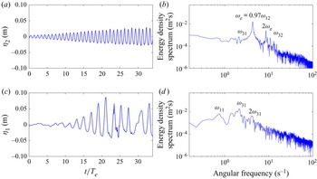
The time histories of free surface and interface displacements near  $x = -a$ (left boundary) are shown in figures 21(a) and 21(c). These displacements are calculated by integrating the VOF function in the vertical direction, because multivalued displacements of the interface may be formed. It can be seen from the figures that resonant response occurs on both free surface and interface as expected, since the frequency of external excitation is equal to twice the third mode of the lower layer natural frequency
 $\omega _{3,1}$ and also is near the first mode of the upper layer natural frequency
 $\omega _{1,2}$. In this case, although resonance can be observed on both surfaces, the displacement of interface near the left boundary is larger than that of free surface most of time, probably because the subharmonic response of the interface absorbs more energy than the harmonic response of the free surface from the external excitation. In addition, the wave crest in the interface is sharper and the trough becomes flatter, resulting from wave nonlinearity.
Displacement of (a) free surface and (c) interface between two layers near the left boundary of a vertically excited tank with  $b_e = 0.2$ m and
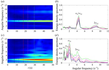
 $\omega _e = 2\omega _{3,1} = 0.97\omega _{1,2}$. (b), (d) The corresponding energy density spectra of numerical results.

Nonlinearity can be further confirmed from the Fourier spectra shown in figure 21(b,d). We can see that for the interface, the dominant frequency of the energy density spectrum is equal to  $\omega _{3,1}=\omega _e/2$ and the second peak corresponds to
 $\omega _{1,1}$. It should be noted that another peak corresponding to
 $2\omega _{3,1}$ can also be seen from figure 21(d), indicating that nonlinearity has been developed in the interface. For the free surface, the dominant frequency of the energy density is equal to
 ${\omega _e=0.97\omega _{1,2}}$, which is approximately equal to twice the main frequency of the wave response at the interface and approaches the first mode of natural frequency related to the upper layer. The second peak, corresponding to
 $2\omega _e$, is excited by nonlinear wave energy transfer.
In order to further investigate the energy transfer mechanism among different modes, we use the wavelet transform technique to study the change of energy density with time (figures 22a and 22c). Five energy density spectra at specific times  $t = 7.5$, 12.5, 17.5, 22.5 and 29.5 s are also drawn in figures 22(b) and 22(d). As can be seen from figure 22(a), for the free surface, the main band corresponds to the frequency of external excitation
 $\omega _e$, which is approximately equal to the first mode of natural frequency related to the upper layer
 $\omega _{1,2}$. This band exists throughout the time and as the amplitude of Faraday waves in the free surface becomes larger, the energy density spectrum also increases as shown in figure 22(b). The second peak is equal to
 $2\omega _e$, and it is not shown until
 $t = 10$ s, from which we can conclude that energy absorbed from external excitation is transferred to this frequency due to wave nonlinearity. For the interface, we can see from figure 22(c) that the main band corresponds to
 $\omega _{3,1}$ and the energy density spectrum of this frequency becomes larger with time (figure 22d); another two peaks corresponding to
 $\omega _{1,1}$ and
 $\omega _{2,1}$ are also found, meaning that the 1st and 2nd mode of natural frequency related to lower layer can also be excited under such vertical oscillation. In addition, a peak equal to
 $2\omega _{3,1}$ does not become significant until
 $t = 15$ s, so the energy absorbed from external excitation is transferred to this frequency in the lower layer because of wave nonlinearity, rather than external excitation, which otherwise should appear from the very beginning.
Wavelet transform analysis of time series of (a) the free surface elevation and (c) the interface elevation near the left boundary when  $b = 0.2$ m and
 $\omega _e = 2\omega _{3,1} = 0.97\omega _{1,2}$, and the energy density spectra obtained from the wavelet transform at
 $t = 7.5$ s (black),
 $t = 12.5$ s (blue),
 $t = 17.5$ s (red),
 $t = 22.5$ s (magenta) and
 $t = 29.5$ s (green).

5. Conclusions
In this study, a multiphase fluid model NEWTANK, which can be employed to track the motion of free surface and interface between different immiscible liquids simultaneously, has been employed to simulate Faraday waves and interface instabilities of two-layer liquids with free surface. Laboratory experiments were conducted for Faraday waves on the free surface and the interface between two liquids under heave excitations in order to study resonance characteristics of the upper layer liquid and to provide reliable data for validation of the numerical model.
It has been found that for two-layer liquids with free surface, when the frequency of vertical external oscillation is equal to or twice the natural frequencies of the system, either for upper layer liquid or lower layer liquid, resonant responses in the form of primary Faraday instabilities can be excited, similar to single-layer Faraday waves. However, for a two-layer liquid system with a free surface, each mode of natural frequency has two values corresponding to free surface and interface, respectively; therefore, the same external vertical excitation may possibly induce upper layer Faraday wave on free surface, lower layer Faraday on interface and Faraday waves on both interface and free surface simultaneously.
Both experiments and numerical simulations are employed to investigate Faraday waves on free surface and the corresponding interface motion. It is found that when the frequency of external excitation is twice the natural frequencies related to upper layer, resonant free surface will be excited at the corresponding modes. The lower layer liquid, although out of the resonant range, will be forced to move with the upper layer liquid, in the same phase but smaller amplitude. When the surface Faraday waves are of second mode response and reach certain wave height, the free surface will go through period tripling breaking, exhibits three-stage secondary instabilities in sequence, similar to those reported earlier for single-layer Faraday waves.
When the frequency of external excitation is twice the natural frequency related to the lower layer liquid, Faraday waves can be induced at the interface of two liquids, whereas the free surface can remain relatively calm. When interface Faraday wave grows over certain threshold, the secondary RT interface instability can be formed even if the lighter liquid is on top of heavier liquid and the excitation amplitude is smaller than gravity. The reason for this phenomenon is that the vertical acceleration of the fluid motion itself induced by interface Faraday wave can grow to certain value, by adding which into the vertical external excitation, the overall effect will overcome the gravity and lead to RT instability on the interface. To quantify the analysis, a new variable called NEGA is proposed in this study to take into account of the fluid acceleration effect in a dynamic fluid system. It is proven that this parameter is a sensible factor to judge whether a two-layer liquid system will be subject to RT instability in a moving tank, i.e. RT instability will occur when NEGA is negative. It is found that the Faraday waves at the interface between fluids are mainly 2-D; however, when secondary interface instability of RT type is generated, the flow structure will transform from 2-D to 3-D.
When resonant responses are generated on both free surface and interface between two liquids, resonances of the upper layer and lower layer with different Faraday modes can lead to reverse flows across the interface and the flow direction of the upper liquid and the lower liquid are opposite at certain instances. During one cycle, the interface will go through the unstable phase when the flows across the interface are different and, thus, induce interface shear and the stable phase when the flows across the interface are in the same direction. The secondary interface instability of KH type will eventually evolve, given that the 2-D Faraday waves grow to certain amplitude, after which the interface will turn from 2-D to 3-D. The transport of energy between different modes and layers are also discussed when the resonance occurs on both layers, indicating that when nonlinearity of resonant response becomes strong enough, the integral times of natural frequency will be excited during the evolution of Faraday waves. More energy will be transferred to higher frequencies as time evolves, due to additional interface mixing by KH instability. However, it should be noted that when instability is generated on free surface or interface, turbulence and surface tension may play an important role, so the stage of post-instability calculation should be validated and analysed further in the future study.
Supplementary movie
Supplementary movie is available at https://doi.org/10.1017/jfm.2022.259.
Acknowledgements
The first author would like to thank Dr G. Chen for his kind and generous assistance in the experiment, and also Mr D. Yan and Y. Wu for their efforts in preparing the experiments and the figures. We would also like to thank three anonymous reviewers who provided critical comments to help us improve the manuscript.
Funding
The research work was supported, in part, by the research grants from Natural Science Foundation of China (grant numbers 51879237 and 52031002), Ministry of Education (grant number G20190023062) and Open Fund of State Key Laboratory of Hydraulics and Mountain River Engineering (grant number SKHL1720).
Declaration of interests
The authors report no conflict of interest.