1. Introduction
In common interest signaling games it is usually the case that precise signaling is better than imprecise signaling in that it allows actors to get better payoffs. Santana (Reference Santana2014) has recently observed that this result does not jibe with systems of natural communication in which ambiguity as to signal meaning is the norm. Santana shows that when signals have some cost and when receivers are able to observe contextual environmental cues, ambiguous signaling strategies can do better than precise ones and can, as a result, evolve. In this note, I show that if one assumes realistic structure on the state space of a common interest signaling game, ambiguous strategies can be explained without appeal to contextual cues. Rather, in many cases, signal cost alone can make ambiguity more effective than precision. This observation is not contra Santana (Reference Santana2014). Some types of ambiguity are well explained by his models and others are better explained by the models presented here.
In section 2, I introduce the sim-max game, the model of common interest signaling appealed to here, and discuss why it is an appropriate model of the sort of real world signaling situations in which ambiguity arises. In section 3, I show that if signal cost is assumed in this model the optimal strategy will involve some level of ambiguity. Finally, I conclude (sec. 4) by briefly discussing payoff-beneficial ambiguity in conflict-of-interest signaling models and then discussing these results and how they should inform our understanding of real world ambiguity.
2. Payoff Structure
A good starting point for models of natural language phenomena is the signaling game introduced by Lewis (Reference Lewis1969).Footnote 1 This game begins when some exogenous force, or ‘nature’, selects a state of the world with some predetermined probability. One agent, called the ‘sender’, is then able to observe this state of the world and send a signal to another agent. This second agent, called the ‘receiver’, observes this signal and is able to take an action in response. If the receiver takes an action that is appropriate for the state of the world, the actors receive a payoff; otherwise they do not.
In signaling games, ambiguous strategies are those in which one signal is used to refer to multiple states of the world. In the Lewis signaling game, ambiguity leads to payoffs that are strictly worse than those for nonambiguous strategies. This is the case because if the sender uses a separate signal in each state, it is possible for the receiver to always select the correct act. If the sender uses an ambiguous signal, however, the receiver is unable to determine which state obtains and thus may sometimes select the incorrect act. Of course, as Lewis (Reference Lewis1969) notes, states in the Lewis signaling game can be thought of as representing larger or smaller groups of real world states. In this way one could reinterpret an ambiguous signaling strategy as nonambiguous by simply reinterpreting the set of states referred to by one signal as a single state. I follow Santana (Reference Santana2014) here by calling ambiguous any signal that refers to multiple states of the world for which it matters from a payoff standpoint. In other words, if an actor uses one signal for multiple states, when multiple signals could allow her to get a better payoff, that signal is ambiguous.Footnote 2
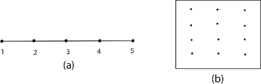
The sim-max game, introduced by Jäger (Reference Jäger2007), builds a natural type of structure into the state space of the Lewis signaling game. In the sim-max game, unlike the Lewis game, it is assumed that states bear similarity relationships to each other. In particular, states are modeled as existing in a metric space where distance represents similarity. For example, a sim-max game might have five possible states of the world modeled on a line (see fig. 1a; fig. 1b shows a similar game with a two-dimensional state space). Because state 1 is closer in state space to state 2 than to state 4, it is assumed that states 1 and 2 are more similar than 1 and 4.
State spaces for sim-max games: a, one-dimensional state space with five states; b, two-dimensional state space with 12 states.

This similarity structure is built into the game through payoff. As in the Lewis game, it is assumed that there is some perfect act for each state of the world that, if taken, will get a perfect payoff for the sender and the receiver. Unlike the Lewis game, however, it is also assumed that a nearly perfect act will get nearly perfect payoffs for these actors. In the example above, act 2 is perfect for state 2 but is also good for states 1 and 3 (because it is assumed that these states are similar to state 2).Footnote 3
This payoff structure mimics many types of real world signaling scenarios. Consider, for example, situations in which one is signaling about color, size, temperature, length, distance, ripeness, hardness, or essentially anything that varies by degree. For each of these properties, there are situations in which a single act will be more or less appropriate for a whole group of states. If one were signaling about the ripeness of a piece of fruit, for example, there would be many states for which eating the fruit would be similarly beneficial and many states for which it would be similarly detrimental. Importantly, this type of situation is one in which ambiguous signaling, in the sense defined here, is often encountered in the real world. One uses the term ‘ripe’ to refer to fruit that is perfect as well as to fruit that is almost rotten despite the fact that the payoffs for eating these two types of fruit are different. To give an example from the animal world, vervets use one alarm call to denote the presence of a hawk, no matter its proximity to the group. This is done despite the fact that a near hawk poses a greater hazard than a far one and that, as a result, different ideal actions might be taken in response to these two states. Given these observations, the sim-max game is an appropriate model of the sort of scenario in which real world ambiguity is often observed.
I will now outline a particular set of games to be considered here. In this set, an additional step is added to the sim-max game. Before nature selects a state to obtain, the sender first chooses a number of possible signals, n. This aspect is added to the model to create a chance for the sender to choose what will essentially amount to a level of ambiguity. Nature then selects the state of the world from the unit interval [0, 1] using a uniform probability distribution.Footnote 4 The sender observes this state and selects a signal from {0, … , n}. The receiver then chooses an act from the unit interval [0, 1]. Payoff for coordination is determined using a function, f, that takes as input the distance, x, between the state of the world and the receiver’s choice. This function will be restricted to only those that are finitely valued over the unit interval (no infinite payoffs) and to those that are strictly decreasing in x. In other words, the less appropriate the act for the state, the lower the payoff. Finally, each signal in this model has a cost, α. This is naturally interpreted as some sort of cognitive cost that the players pay for the ability to send and receive signals. This means that if a sender chooses n signals, the payoff for both players for a round of play will be f(x) − nα.
3. Ambiguity and Signal Cost
In the model just described, the actors do best to use a signaling strategy that is as unambiguous as possible when there is no signal cost: α = 0. This is the case because the actors can obtain the best payoff in each state by selecting the exact right act (assuming, as we do, that payoff decreases strictly in x). What this means is that when there is no signal cost, the optimal signaling strategy employs an infinity of signals. One can show, though, that if α > 0, no matter how small, some level of ambiguity will be beneficial to actors from a payoff standpoint. In particular, the optimal strategy will now involve the use of a finite number of signals to represent the infinite possible states.
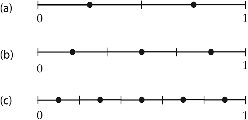
In order to see why this is the case, it will first be useful to discuss optimal strategies in sim-max games in which the number of signals is exogenously restricted. Obviously in such games, the actors cannot assign a separate signal for each state, and so ambiguity is necessary, even if a nonambiguous strategy would get a better payoff. Jäger et al. (Reference Jäger, Metzger and Riedel2011) show that optimal strategies in these games, which Jäger calls ‘Voronoi languages’, are “as separating as possible” (5).Footnote 5 In a Voronoi language, senders divide the state space of the game into convex cells and attach a signal to each one of these. Receivers then take an act in response to each signal that is approximately appropriate for all the states in the associated cell. If, as in the games considered here, the state space is a line and there is a uniform probability distribution over states, the sender using a Voronoi language will divide the state space into cells of the same length, and the receiver will choose acts appropriate for the middle of each cell. Figure 2 shows representations of Voronoi languages for the unit interval with various signal numbers. For a much more detailed description of Voronoi languages, including their properties in multidimensional state spaces, see Jäger et al. (Reference Jäger, Metzger and Riedel2011).
Voronoi languages of sim-max games in which the state space is the unit interval: a, language with two signals; b, three signals; c, five signals. In each case, the line represents the state space, the bars mark out cells in the state space for which one signal is sent, and the dots represent the receiver’s acts in response to the signal associated with each cell.

Let us return to the proposed model and give a proof sketch of why ambiguity is payoff beneficial in these games whenever α > 0 (for the full proof, see the appendix). It is enough to show that actors who play otherwise optimal strategies maximize payoff with respect to the number of signals, n, for some finite n whenever α > 0. For a given n, the best strategy for the actors is the Voronoi language described above. It can be shown that as one increases n stepwise, there is a payoff increase at each stage for using a Voronoi language with higher precision (a greater number of signals and thus less ambiguity). However, each added signal increases payoff less than the one before it and, in fact, this increase approaches 0 as n approaches ∞. Because the cost for signals increases linearly (i.e., by α at each step), there must then be a step where α is greater than the increase due to precision. From this step forward, any increase in n will cause a decrease in overall payoff. Thus, there is some finite n that maximizes payoff in the game.Footnote 6
One might note that the assumption that signal cost is always constant is a strange one given the proposed interpretation. It might make more sense to suppose that as an actor invests in the cognition necessary to signal, her costs decrease for each signal added. After all, while vervets might incur some significant cognitive cost to add a new signal to their repertoire, the addition of an extra word to some human’s vocabulary is presumably much smaller. Note that the proof sketched above may be extended to cases in which signal cost is decreasing. (For this extension and a discussion of optimal strategies in these cases, see the appendix.)
The proof just sketched depends on the state space of the game being infinite, but in most real world situations the number of states for which different actions lead to different payoffs will be finite. This proof should not be thought of as applying directly to real world scenarios but as illustrating a phenomenon that does—when there are a large number of states of the world, and signals have some cost, using enough signals to fully differentiate states will not be an effective strategy. Along these lines, similar results can be obtained for finite state spaces. For some parameter settings of a finite game that is otherwise similar to the one described above—few states, low signal cost, and a sharp decrease in payoff for the wrong act—there will be no ambiguous strategy that can outperform a nonambiguous strategy. But for other parameter settings—many states, higher signal cost, and more flexibility as to which act is performed—ambiguity at some level will be optimal. In real world signaling scenarios, the number of states is often very large. What this means is that in many real world settings, it will be the case that some level of ambiguity will be beneficial, assuming a cognitive cost for signal use.
To give an example of a finite sim-max game in which ambiguity is payoff optimal, consider one with 100 states and acts and f(x) = 100 − x.Footnote 7 When α = 5, payoff for this game is optimized when actors play a Voronoi language with n = 2. When α = 1, payoff is maximized for n = 5. If one considers a game with 1,000 states/acts, a payoff function f(x) = 1,000 − x and α = 1, payoff is maximized for n = 16.
4. Many Ambiguities
Before discussing the analysis above, it should be noted that there have been previous results that can explain ambiguity by appeal to conflict-of-interest signaling games. In these games, unlike the Lewis signaling game or the sim-max game, sender and receiver do not always get the same payoff and so may prefer different acts to be taken in the same state. For example, Crawford and Sobel (Reference Crawford and Sobel1982) present a model that is similar to the game presented here in that the state space is continuous but where (1) there is no signal cost and (2) actors may have conflicting interests. These authors show that at equilibria the signals chosen by the actors, in many cases, are ambiguous. In particular, the sender partitions the state space and sends a different signal for each partition. While this strategy is similar to the optimal strategies for the games presented here, ambiguity is payoff beneficial for a different reason. In Crawford and Sobel’s model, the sender benefits by obscuring the true state from the receiver so that the receiver will sometimes choose a state that the sender (but not the receiver) prefers. In other words, the sender strategically transfers only some, but not all, of the information available to her. Similar results have been replicated in many models and seem to explain cases of ambiguity where interests conflict. For example, consider a man who would like to conceal his age from a partner who would like to know it. When asked, he might reply, “well, I’m not 25 anymore.” This statement is ambiguous to the man’s advantage since his interactive partner might take him to be younger than he is.
In cases of common interest signaling, however, ambiguity is also observed, and results from conflict-of-interest models do not directly apply. As argued, the model presented here is a simple model of a type of common interest scenario in which signaling ambiguity is often seen. I have shown that signal cost in this model means that the optimal strategy will be ambiguous. This differs from the analysis of ambiguity provided by Santana (Reference Santana2014), which appeals to both signal cost and context to explain the evolution of this signaling phenomenon. Although in some ways the explanation of ambiguity provided here is simpler, this does not mean that there is reason to think Santana’s results are not important in explaining linguistic ambiguity.
Different types of ambiguity seem to be better explained by one or the other of these models. In some real world cases, a signal is ambiguous in that it represents a set of states for which the same action works fairly well but for some of which a slightly different action might be better. Examples of this are situations like the ones used to motivate the models here. The vervet hawk alarm is ambiguous in that it represents many states where a hawk is present. Some of these might be better responded to with slightly different actions (dive for the nearest bush rather than take the time to run to that really thick undergrowth), but for the most part the same actions will be at least partly appropriate. This type of ambiguity is not strongly context dependent. These types of situations are well represented by the models presented in this note.
But, for some types of ambiguity, taking the same action in response to an ambiguous signal will be unsuccessful. Consider, for example, a term like ‘dangerous’. One might describe both a rattlesnake and a scheming coworker as dangerous, but taking the same action in response to these two situations (trying to outpolitick the rattlesnake or remove the colleague from your path with a long, forked stick) will lead to poor payoffs. This type of ambiguity is better represented by Santana’s models in which the receiver uses contextual clues to determine how to interpret the signal.
In the first type of case outlined—in which ambiguous signals cover states that are similar with respect to payoff—there is a sort of true ambiguity for the receiver. The receiver can act successfully without ever knowing what state obtains. In the second sort of case, the signal is ambiguous, but the receiver solves the coordination problem by using other information. In other words, the receiver knows what state obtains, despite receiving an ambiguous signal. This aspect is captured in Santana’s models. Nature is assumed to provide enough information to the receiver to allow her to choose the uniquely correct state. In the models I provide, this is obviously not the case.Footnote 8 From these observations it should be clear why both models of ambiguity are helpful in that they shed light on two related types of natural language phenomena.
Santana (Reference Santana2014) shows not only that ambiguity is optimal from a payoff standpoint in the models he presents but that it is expected to evolve under the replicator dynamics with mutation. No evolutionary analysis is given here. The results presented, however, provide mathematical justification for the intuitive observation that to maintain separate signals for every possible payoff-relevant real world state would be prohibitively costly. Given this, one should expect the evolution of some level of ambiguity in natural signaling scenarios. In particular, more ambiguity should be expected when it is costly for the actors to maintain many signals and when there are many different payoff-relevant states. The models presented also highlight the reason why ambiguity of this sort can be a successful strategy in its own light—when a set of states all can be responded to with the same act, to decent results, ambiguity is kinda good enough.
The results presented here correspond nicely with the intuition that ambiguity is a result of a trade-off between a need to minimize cognitive complexity and a desire for terms to be maximally informative. Van Benthem (Reference van Benthem, Borgers, van Benthem and Rubsenstein2001), for example, points out that “many people (including myself) believe that natural language strikes some kind of successful balance between expressive power for information content and resource complexity of cogitation and communication processes” (95). Van Benthem goes on to contrast this with game theoretic approaches to language that focus on optimization of payoff. The analysis here, and that provided by Santana, indicates that these approaches need not stand in opposition to each other. Rather a payoff-optimal language will itself include some balance between cognitive cost and expressive power.
Appendix
Consider a sim-max game with a set of states S = [0, 1], a set of acts A = [0, 1], and a countably infinite set of possible signals M. Assume that nature chooses states using a uniform probability distribution. A sender strategy is defined as a choice of the number of signals used, n, and a complete contingent plan of action given n. A receiver strategy is defined as a complete contingent plan of action given n. Payoff for action is determined by a function f(x), where x = |s − a| with s nature’s choice of state and a the receiver’s choice of act. Assume that f(x) is strictly decreasing and bounded for [0, 1]. Further assume some cost, α, for each signal used. Payoff for both actors is thus f(x) − nα.
Proposition. The optimal strategy choice for two actors playing this game involves a finite choice of n.
Proof. Given some n the optimal strategy for actors in the described game is the Voronoi language (where cells are of size 1/n and the receiver’s choice of acts correspond to the center of each cell; Jäger et al. Reference Jäger, Metzger and Riedel2011). Suppose one increases n stepwise, considering at each step the expected payoff for the Voronoi language with n signals.
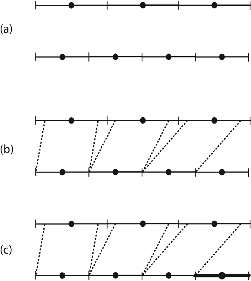
I claim that at each step n, the actors will only increase expected payoff for 1/n of the state space. To see why this is the case for any particular step n, consider the Voronoi languages for (n − 1) and n. At (n − 1), the state space is divided into n − 1 cells of size 1/(n − 1). At n, the state space is divided into n cells of size 1/n. Note that a cell of size 1/n in the n language is identical, from a payoff perspective, to the same length center portion of a cell of size 1/(n − 1) in the (n − 1) language. For this reason, one can associate (n − 1) of the cells at step n with the center of each cell at step (n − 1). Each of these cells will receive the same expected payoff as the centers of the (n − 1) cells. The remaining cell in the n step is the only section of the state space at that step that may receive a greater expected payoff. This cell is of size 1/n (see fig. A1 for a graphic representation of this).
Representation of the argument that expected payoff can only improve for 1/n of the state space when one moves from a Voronoi language of size n − 1 to one of size n. Step from n = 3 to n = 4 shown: a, the two Voronoi languages at these steps; b, one can associate three of the four cells in the n = 4 language with the centers of the cells in the n = 3 language; expected payoff will be identical for the associated areas; c, the remaining area of the n = 4 state space is highlighted; this is the only area where the expected payoff will not be identical to some area of the n = 3 language and thus the only area where payoff may improve.

Let m be the difference between the supremum of f(x) in [0, 1] and the infimum of f(x) in [0, 1]. Given two sets of sender and receiver strategies, the greatest payoff difference for one state in the game under these strategies will be m. Because payoff can only change for 1/n of the state space at each step n, the change in expected payoff for the Voronoi language at n − 1 and that at n can be no greater than (1/n)m.
As n → ∞, (1/n) → 0. Given that f(x) is bounded on [0, 1], m is finite; m is a constant and so is also independent of n. Then (1/n)m → 0 as well. Signal cost α is positive, and independent of n, and so at some step it must be the case that α > (1/n)m. At every step thereafter, the payoff for choosing (n + 1) signals will be less than for choosing n. Thus the optimal strategy in this game involves choosing a finite n. QED
In fact, the argument given above proves something considerably stronger. Consider a game as described but where signal cost is determined by some function c(n). Payoff is then  . Let h(n) = (1/n)m.
Proposition. In all games where there exists some integer n* such that for all integers n > n* it is the case that c(n) > h(n), the optimal strategy choice involves a finite choice of n.
Proof. Let x(n) be the expected payoff for a Voronoi language with n signals. Now choose any n > n*. The payoff for having n signals must be less than  because h(i) < c(i) for each i in the sums. Thus payoff for any n > n* is less than for n*. Because n* is finite, the optimal signal choice must be finite too. QED
Note that this will hold even for decreasing c(n) as long as it is the case that c(n) is greater than h(n) for all sufficiently large n.
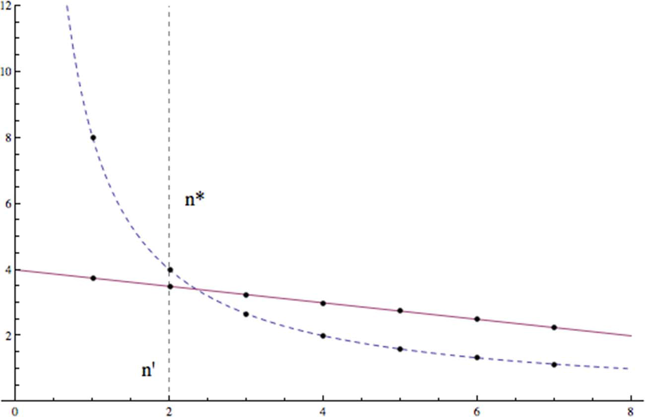
The exact value of the optimal, finite n, call this value n′, for such a game will depend on the particulars of f(x) and of c(n), but it will be the case that n′ < n*. It is difficult to say more about n′ generally, but some discussion, and a figure, may add clarity. Because m is a constant, h, which represents the upper bound on the payoff increase that a signal can provide, is convex and decreasing. Let b(n) be a function that outputs the expected payoff increase for adding signal n. The exact form of b(n) will depend on the payoff function, but for simplicity sake it is represented by the dashed line in figure A2, which is convex and decreasing. Signal cost, c(n), is represented in this figure by the solid line, although c could take any form.
Example case in which although signal cost is decreasing, ambiguity is still payoff beneficial. Dashed line represents the benefit of adding additional signals, b(n), while the solid line represents the cost, c(n). Dotted line represents n*, the integer where for all integers n > n*, c(n) > b(n). In this case, n* is also the optimal number of signals n.

If one imagines increasing n stepwise, n′ will occur at the last step where the benefits from b(n) outweigh the costs of c(n). If it is the case that for all integers n < n*, c(n) < b(n) and for all integers n > n*, c(n) > b(n), n′ = n* (see fig. A2 for an example). If, however, c(n) and b(n) cross at multiple points, things will be a bit more complicated. In our stepwise process, let n′′ be the last signal added (i.e., the last signal that provided a payoff benefit). It will be beneficial to add a higher number n if the sum of the benefits outweighs the sum of the costs between n′′ and n or if  . The last integer for which this is the case will be the optimal number of signals, n′.