INTRODUCTION
Variation in the geochemical composition of marine sediments conveys information on climatic and oceanographic variations (Calvert and Pedersen, Reference Calvert and Pedersen2007). Elemental data derived from marine sediments have been used to reconstruct the terrestrial climate and sediment source area characteristics (Lupker et al., Reference Lupker, France-Lanord, Galy, Lavé and Kudrass2013; Pérez-Cruz, Reference Pérez-Cruz2013; Clift et al., Reference Clift, Wan and Blusztajn2014). Specific elements, for example, aluminum (Al), iron (Fe), titanium (Ti), and potassium (K), have been interpreted to indicate terrigenous input by either river or eolian dust in different environmental settings (Peterson et al., Reference Peterson, Haug, Hughen and Röhl2000; Bozzano et al., Reference Bozzano, Kuhlmann and Alonso2002; Adegbie et al., Reference Adegbie, Schneider, Röhl and Wefer2003). However, the absolute contents of specific elements can be influenced by dilution effect and hydrodynamic differentiation; elemental ratios have been used more widely than a single elemental signal (Weltje and Tjallingii, Reference Weltje and Tjallingii2008). Among elemental ratios, calcium/aluminum (Ca/Al), calcium/iron (Ca/Fe), and calcium/titanium (Ca/Ti) are the mostly commonly adopted to represent marine and fluvial end members in different regions (Arz et al., Reference Arz, Pätzold and Wefer1998; Blanchet et al., Reference Blanchet, Tjallingii, Frank, Lorenzen, Reitz, Brown, Feseker and Brückmann2013; Revel et al., Reference Revel, Colin, Bernasconi, Combourieu-Nebout, Ducassou, Grousset and Rolland2014; Bouimetarhan et al., Reference Bouimetarhan, Dupont, Kuhlmann, Patzold, Prange, Schefuss and Zonneveld2015). Among terrigenous elemental ratios, potassium/aluminum (K/Al) and silicon/aluminum (Si/Al) are the most frequently applied to indicate the chemical weathering intensity in the source area (Yarincik et al., Reference Yarincik, Murray and Peterson2000; Bayon et al., Reference Bayon, Dennielou, Etoubleau, Ponzevera, Toucanne and Bermell2012; Bloemsma et al., Reference Bloemsma, Zabel, Stuut, Tjallingii, Collins and Weltje2012).
In spite of the wide application of the geochemical composition of sediments in paleoclimatic studies, several other factors can influence the geochemical signals in marine sediments. Indicators for fluvial discharge, such as Ca/Al ratios, are not only influenced by climatic conditions in the hinterland, but also by (1) sea-level fluctuation, (2) carbonate production, and (3) carbonate dissolution in the adjacent ocean (e.g., van der Lubbe et al., Reference van der Lubbe, Tjallingii, Prins, Brummer, Jung, Kroon and Schneider2014). Geochemical properties of terrigenous sediments may be affected by grain-size variations (Bouchez et al., Reference Bouchez, Gaillardet, France-Lanord, Maurice and Dutra-Maia2011; Meyer et al., Reference Meyer, Davies and Stuut2011), as well as other factors including provenance, weathering, and physical and chemical modification that occur during the source to sink process (Govin et al., Reference Govin, Holzwarth, Heslop, Keeling, Zabel, Mulitza, Collins and Chiessi2012; Garzanti et al., Reference Garzanti, Padoan, Setti, López-Galindo and Villa2014). For example, apart from the weathering indication, Si/Al ratio is also affected by the hydraulic sorting effect, which may cause biased results for weathering indication (Just et al., Reference Just, Schefuss, Kuhlmann, Stuut and Pätzold2014). Bloemsma et al. (Reference Bloemsma, Zabel, Stuut, Tjallingii, Collins and Weltje2012) provided a statistical method to separate the grain-size-dependent part of compositional variation from a residual part; however, this method depends on the specific geologic setting. Thus, it is necessary to evaluate the factors that influence and/or control the geochemical signature of marine sediments in different geologic settings. To date, research in this field is not well established for the East African continental margin. Here we present a multiproxy data set from a high-resolution marine sediment core offshore Tanzania to investigate (1) the sources of geochemical elements, (2) the influence and/or control of physical (grain-size) parameters on geochemical composition, and (3) their implications for East African climatic and sea-level changes during the Holocene.
REGIONAL SETTING
The Pangani River
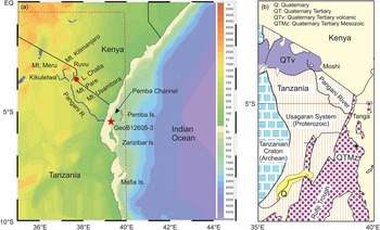
The Pangani River is ~500 km long with two major tributaries (Fig. 1a): the Ruvu and Kikuletwa (Hellar-Kihampa et al., Reference Hellar-Kihampa, Potgieter-Vermaak, Van Meel, Rotondo, Kishimba and Van Grieken2012). This river system passes through the Pare and Usambara mountain ranges before reaching the western Indian Ocean (WIO; Komakech et al., Reference Komakech, van Koppen, Mahoo and van der Zaag2011). The Pangani delta is considered to be the major supplier of freshwater (1830 mm3/yr) and siliciclastic sediments in the investigated region (Shaghude, Reference Shaghude2007). The upstream region of the Pangani River is covered by huge volcanic massifs of the Mt. Kilimanjaro and Meru (Fig. 1b; Kashaigili, Reference Kashaigili2010). The central drainage area is composed of Proterozoic crystalline rocks (Usagaran System; Fig. 1b) consisting of granulitic gneisses (Sommer et al., Reference Sommer, Kröner, Hauzenberger, Muhongo and Wingate2003; Bauernhofer et al., Reference Bauernhofer, Hauzenberger, Wallbrecher, Muhongo, Hoinkes, Mogessie, Opiyo-Akech and Tenczer2009), whereas the coastal area is dominated by Mesozoic and younger marine sediments (Kapilima, Reference Kapilima2004).
(color online) (a) The Pangani River Basin. The location of core GeoB12605-3 is indicated by the solid star. (b) A simplified geologic map of east Tanzania, modified from Semkiwa and Hester (Reference Semkiwa and Hester2005). The area of panel b is indicated by the rectangle in panel a.

Climatic setting
Modern climate
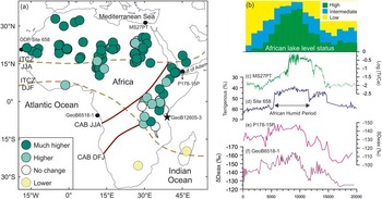
The present climatic system of East Africa is influenced by the strong seasonal monsoon climate: the southeast monsoon occurs during June–August, and the northeast monsoon during December–February (Beal et al., Reference Beal, Hormann, Lumpkin and Foltz2013). Driven by the migration of the Intertropical Convergence Zone (ITCZ; dashed lines in Fig. 2a), there are two distinct rainy seasons during the monsoonal transition: the long rains (March–May) and the short rains (September–November). In addition, the area is influenced by the Congo Air Boundary (CAB; solid lines in Fig. 2a), separating the air masses containing moisture derived from the Atlantic and Indian Oceans (Nicholson, Reference Nicholson1996). This seasonal reversal in the wind patterns cause phases of upwelling in the northern region off East Africa (McClanahan, Reference McClanahan1988). In contrast, surface waters south of 4°S are stratified year-round and characterized by relatively low benthic productivity and nutrient content (Birch et al., Reference Birch, Coxall, Pearson, Kroon and O’Regan2013).
(color online) (a) Modern climatic system of East Africa, with lake-level reconstructions at 9 ka by Tierney et al. (2011a). Locations of the Intertropical Convergence Zone (ITCZ; dashed lines) and the Congo Air Boundary (CAB; solid lines) for June–August (JJA) and December–February (DJF) are represented. (b) African lake–level status in basins in East and North Africa adapted from deMenocal and Tierney (Reference deMenocal and Tierney2012). (c) Log ratios of Ti/Ca from core MS27PT off the Nile Delta, representing marine versus terrigenous sedimentation (Revel et al., Reference Revel, Colin, Bernasconi, Combourieu-Nebout, Ducassou, Grousset and Rolland2014). (d) Ocean Drilling Program (ODP) Site 658 dust flux (deMenocal et al., Reference deMenocal, Ortiz, Guilderson, Adkins, Sarnthein, Baker and Yarusinsky2000). (e) δDwax data from Gulf of Aden core P178-15P (Tierney and deMenocal, Reference Tierney and deMenocal2013). (f) Congo River outflow inferred from δD of leaf waxes (Schefuß et al., Reference Schefuß, Schouten and Schneider2005).

The Holocene African Humid Period
During the Holocene, Africa experienced rapid hydrologic fluctuations, with a more pluvial early to middle Holocene (12–5 ka) as indicated in numerous records (Fig. 2b–f). This relatively humid period, termed the African Humid Period (AHP; Fig. 2d; deMenocal et al., Reference deMenocal, Ortiz, Guilderson, Adkins, Sarnthein, Baker and Yarusinsky2000), extends from North Africa to as far south as 10°S in East Africa (Fig. 2a; Gasse, Reference Gasse2000; Tierney et al., Reference Tierney, Lewis, Cook, LeGrande and Schmidt2011a). Following the occurrence of the AHP, significant hydrologic changes have occurred throughout the African continent, such as the Green Saharan, and the high stand in lake levels in the East African Rift Valley (e.g., Kröpelin et al., Reference Kröpelin, Verschuren, Lézine, Eggermont, Cocquyt, Francus and Cazet2008; Junginger et al., Reference Junginger, Roller, Olaka and Trauth2014; Morrissey and Scholz, Reference Morrissey and Scholz2014; Fig. 2a and b). The AHP was also associated with enhanced runoff of large rivers, such as the Nile River (Fig. 2c; Blanchet et al., Reference Blanchet, Tjallingii, Frank, Lorenzen, Reitz, Brown, Feseker and Brückmann2013; Revel et al., Reference Revel, Colin, Bernasconi, Combourieu-Nebout, Ducassou, Grousset and Rolland2014) and the Congo River (Fig. 2f; Schefuß et al., Reference Schefuß, Schouten and Schneider2005). In addition, there is a hinge zone near Lake Malawi, where sites located to the north of the lake experienced a wetter early Holocene, whereas southern sites were relatively dry (Fig. 2a; Gasse, Reference Gasse2000). The AHP ended with an abrupt termination, as inferred from a sudden increase in dust fluxes around 5.5 ka (Fig. 2d; deMenocal et al., Reference deMenocal, Ortiz, Guilderson, Adkins, Sarnthein, Baker and Yarusinsky2000) and increases in hydrogen isotope values in leaf wax around 5 ka (Fig. 2e; Tierney and deMenocal, Reference Tierney and deMenocal2013). In contrast, the termination of the AHP as recorded in sediments offshore the Nile and Congo River mouths shows a more gradual pace (Fig. 2c and f; Schefuß et al., Reference Schefuß, Schouten and Schneider2005; Revel et al., Reference Revel, Colin, Bernasconi, Combourieu-Nebout, Ducassou, Grousset and Rolland2014).
The pace of the AHP over East Africa, the East African Humid Period (EAHP), is inconsistent in both timing and abruptness, according to the existing paleoclimatic records and is still a matter of debate (Castañeda et al., Reference Castañeda, Schouten, Pätzold, Lucassen, Kasemann, Kuhlmann and Schefuß2016). Though the expression of the EAHP appears highly variable in space and time, a general pattern can be deduced: a significant humid period from the early Holocene to ~8 ka (EAHP I; Costa et al., Reference Costa, Russell, Konecky and Lamb2014) and a second moderate humid phase between 8 and 5 ka (EAHP II) during the mid-Holocene (Blanchet et al., Reference Blanchet, Contoux and Leduc2015). The second humid phase ended with an abrupt or gradual termination (Revel et al., Reference Revel, Colin, Bernasconi, Combourieu-Nebout, Ducassou, Grousset and Rolland2014; Castañeda et al., Reference Castañeda, Schouten, Pätzold, Lucassen, Kasemann, Kuhlmann and Schefuß2016; Liu et al., Reference Liu, Rendle-Bühring, Kuhlmann and Li2017), followed by an arid late Holocene (Fig. 2).
MATERIALS AND METHODS
Materials
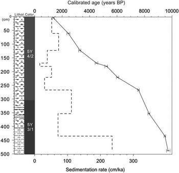
Core GeoB12605-3 (5°34.39′S, 39°06.49′E; seawater depth 197 m) was drilled in the Pemba Channel off the Pangani River mouth during the R/V METEOR Cruise M75/2 in February 2008 (Savoye et al., Reference Savoye, Ridderinkhof, Pätzold and Schneider2013). Total core length is 500 cm, and sediments grade from dark-gray fine-grained siliciclastic muddy sediments to olive-gray mixed biogenic calcareous-siliciclastic sandy sediments from the core base to top (Fig. 3). A detailed age model was established based on 10 radiocarbon ages measured on the planktonic foraminiferal shells by Kuhnert et al. (Reference Kuhnert, Kuhlmann, Mohtadi, Meggers, Baumann and Pätzold2014). Radiocarbon ages were converted into calendar years with the CALIB program (Calib 6.0), using the calibration curve marine 09 (ΔR= 150±60). ΔR is based on the 10 geographically closest calibration points, omitting the very young age from Watamu Reef (Grumet et al., Reference Grumet, Guilderson and Dunbar2002) and one extremely old age from the Seychelles (Southon et al., Reference Southon, Kashgarian, Fontugne, Metivier and Yim2002). Thus, the weighted average was calculated from the remaining 8 calibration points. According to the age model, core GeoB12605-3 covers a period spanning from 9.7 to 1.3 ka. In general, sedimentation rates are high (~60 cm/ka on average; Fig. 3), and a decrease in the sedimentation rate is observed from the base to the top of the core (Liu et al., Reference Liu, Rendle-Bühring, Meyer and Henrich2016).
Age model (solid line) and down-core variations in sedimentation rates (dashed line) of core GeoB12605-3, modified from Kuhnert et al. (Reference Kuhnert, Kuhlmann, Mohtadi, Meggers, Baumann and Pätzold2014) and Liu et al. (Reference Liu, Rendle-Bühring, Meyer and Henrich2016). Error bars mark the ±1 sigma range.

Grain-size analysis
The grain size of 224 terrigenous subsamples, extracted from marine bulk sediments, was analyzed at 2 cm intervals and measured with a Beckman Coulter Laser Diffraction Particle Size LS200. The grain-size spectra were resolved between 0.4 and 2000 μm in 92 size classes. The terrigenous fraction was obtained by treating bulk sediment with 10 mL hydrochloric acid (HCl; 10%) to remove CaCO3, 10 mL 35% hydrogen peroxide (H2O2) to remove organic matter, and 6 g sodium hydroxide (NaOH) to remove biogenic opal. Finally, each sample was boiled with ~300 mg of sodium pyrophosphate (Na4P2O7∙10H2O) before measurement to avoid the formation of aggregates. Down-core volume percentages of selected grain-size fractions were calculated: (1) clay (<2 µm); (2) silt (2–63 µm); (3) finer sands (63–250 µm), which included very fine sand (63–125 µm) and fine sand (125–250 µm); and (4) coarser sands (250–2000 µm), which included medium sand (250–500 µm), coarse sand (500–1000 µm), and very coarse sand (1000–2000 µm) fractions.
Elemental composition
Bulk sediment samples were stored at −20°C at the IODP Bremen Core Repository (MARUM, University of Bremen) for 24 hours. Then samples were freeze-dried, and ~4 g of dry bulk sediment was ground with an agate mortar to ensure the sediments were homogenous. The powder was loosely packed in a sample cup covered with a 4-µm-thick prolene foil, and the remaining space in the cup was filled by a foam plug prior to measurement (Govin et al., Reference Govin, Holzwarth, Heslop, Keeling, Zabel, Mulitza, Collins and Chiessi2012). A geochemical analysis of the pretreated samples was performed on a Spectro Xepos EDP-XRF at the Geochemistry Department of the Geosciences Faculty at the University of Bremen. The device was operated with the software Spectro X-Lab Pro (Version 2.4) using the Turboquant method of Schramm and Heckel (Reference Schramm and Heckel1998). The analytical quality of the measurements was evaluated using the certified standard reference material MAG-1, and measured values within 1% were accepted. The concentrations of specific elements (Mg, Al, Si, K, Ca, Ti, Fe, and Sr) of the bulk sediment were measured with a sample resolution of 2 cm.
Principal component analysis
In order to classify the major geochemical elements and determine their source and the influence and/or control of physical (grain-size) parameters on their composition, we performed a principal component analysis (PCA) on geochemical data by using XLSTAT software.
RESULTS
Grain-size distribution
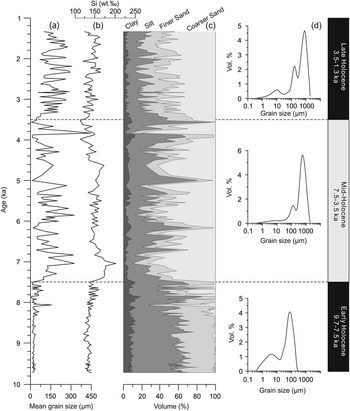
A comparison of the grain-size distribution pattern with depth and concentration of silicon shows several trends (Fig. 4). In general, there is an increase in the mean grain size (Fig. 4a) from the base to the top of the core. The sand fraction represents 45%, 64%, and 75% of terrigenous sediment during the early, middle, and late Holocene, respectively, and the silt fraction accounts for 47%, 30%, and 21% of the terrigenous sediment during the early, middle, and late Holocene, respectively (Fig. 4c).
Grain-size results for core GeoB12605-3. (a) The mean grain size of the terrigenous component of the marine sediment. (b) Concentration of silicon. (c) Down-core volume percentage of clay (<2 µm), silt (2–63 µm), finer sand (63–250 µm), and coarser sand (250–2000 µm) fractions in the terrigenous sediment. (d) The representative grain-size distribution patterns during respective time intervals.

The grain-size distribution reveals that the lower sequence (>264 cm), older than 7.5 ka, is platykurtic, with a main mode oscillating between 80 to 100 µm (very fine sand) and a secondary mode in the silt fraction (Fig. 4d). Since 7.5 ka, the grain-size distribution pattern is trimodal, with a main mode ~800 µm (coarse sand), which persists to the end of the core (Fig. 4d). According to grain-size signal, three main phases can be defined (Fig. 4): the early Holocene (9.7–7.5 ka; 488–266 cm), the mid-Holocene (7.5–3.5 ka; 264–132 cm), and the late Holocene (3.5–1.3 ka; 130–2 cm).
Geochemical composition
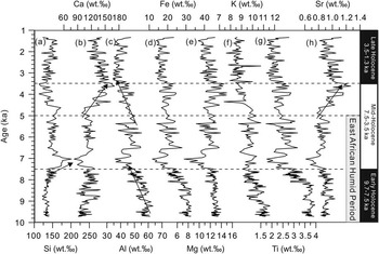
Si and Ca are the most abundant elements, with average concentrations of 140 wt.‰ and 120 wt.‰, respectively. Al, Fe, and Mg represent the elements with the second highest concentrations, with mean values of 48 wt.‰, 23 wt.‰, and 12 wt.‰, respectively. Average concentrations of K and Ti are 10 wt.‰ and 3 wt.‰, whereas Sr is usually lower than 1 wt.‰ (Fig. 5).
Concentrations of elements from core GeoB12605-3 against the time: silicon (a), calcium (b), aluminum (c), iron (d), magnesium (e), potassium (f), titanium (g), and strontium (h). Arrows represent the main change trends of respective elements. Dashed lines represent the boundary between the early, middle, and late Holocene.

From down-core variations in elemental concentrations, a number of trends are observed (Fig. 5). Si exhibits a consistently low concentration during the early Holocene, followed by a rapid increase in concentration at the end of the early Holocene (Fig. 5a). These high concentrations continue to be maintained and end with a steady decrease to the end of the mid-Holocene (~3.5 ka). Since then, the concentration of Si shows a steady slight increase throughout the late Holocene. Concentrations of Ca and Sr show no significant fluctuations during the early and the early mid-Holocene. Around 5 ka (the end of EAHP), the relative abundance of Ca and Sr in the bulk sediment increases rapidly to the end of the mid-Holocene (3.5 ka; Fig. 5b and h). Since then, Ca and Sr concentrations decline gradually throughout the late Holocene. Al, Fe, K, and Ti share very similar changing trends (Fig. 5c, d, f, and g), with the highest concentrations during the early Holocene and a decrease during the late early Holocene. All these elements recover to a moderate level followed by a steady decrease to the end of mid-Holocene (~3.5 ka). In the late Holocene, concentrations of Al, Fe, K, and Ti are stable and consistently low. Mg shows relative consistency with a significant decrease at the end of the early Holocene (Fig. 5e).
PCA results
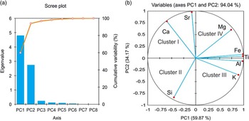
A scree plot and a correlation circle summarizing the PCA results are shown in Figure 6. The first two principal components account for 94.04% of the total variance: 59.87% and 34.17% of the variance for principal component 1 (PC1) and principal component 2 (PC2), respectively (Fig. 6a). PC1 is strongly influenced by high values in Al, Fe, K, and Ti, which are clustered together and have high positive loadings on the PC1 axis. In contrast, PC2 shows high positive loadings for Sr and Ca on the negative PC1 axis. Si shows a negative correlation with PC1 and PC2, whereas Mg displays a positive correlation with PC1 and PC2 (Fig. 6b). According to the loadings of the elements on PC1 and PC2, four basic clusters for elements can be identified: cluster I (Ca and Sr), cluster II (Si), cluster III (Al, Fe, K, and Ti), and cluster IV (Mg).
(color online) Principal component analysis results of major elements. (a) Scree plot. (b) Correlation circle. PC, principal component.

DISCUSSION
Source of major elements
Marine sediments consist of both terrigenous and marine biogenic components. According to the PCA results, each element is categorized to one of the four clusters. For cluster I, Ca in marine sediments commonly represents the biogenic carbonate component (Arz et al., Reference Arz, Pätzold and Wefer1998; Stuut et al., Reference Stuut, Temmesfeld and De Deckker2014), which is derived from carbonate-secreting organisms. Sr occurs in both terrigenous and marine minerals; however, our PCA results (Fig. 6b) suggest that most of the Sr originates from marine biogenic carbonate. Thus, Ca and Sr (Cluster I) are most plausibly interpreted to represent the biogenic component in the Tanzanian shelf sediments.
For cluster II, Si is contained in all clay minerals, but also in coarser-grained quartz grains (Govin et al., Reference Govin, Holzwarth, Heslop, Keeling, Zabel, Mulitza, Collins and Chiessi2012). In our results, Si shows a negative correlation to all the other elements, indicating that Si has a significant dilution effect on other elements. The concentration of Si shows a similar changing trend to that observed in the grain-size pattern (Fig. 4a and b). This suggests that the distribution of Si in the studied sediments is related to the concentration of the coarser-grained minerals, such as terrigenous quartz and feldspar (Liu et al., Reference Liu, Rendle-Bühring, Meyer and Henrich2016). In cluster III, Al, Fe, K, and Ti represent terrigenous components in the marine sediments (Krom et al., Reference Krom, Stanley, Cliff and Woodward2002; Hellar-Kihampa et al., Reference Hellar-Kihampa, Potgieter-Vermaak, Van Meel, Rotondo, Kishimba and Van Grieken2012). These four elements might be enriched in different mineral phases: Fe can be incorporated into clay minerals such as chlorite, smectite, and illite (Cantalejo and Pickering, Reference Cantalejo and Pickering2014), while K is mostly associated with K-feldspar or illite (Kuhlmann et al., Reference Kuhlmann, Meggers, Freudenthal and Wefer2004). For cluster IV, Mg in marine sediments is usually accompanied by clay minerals (e.g., illite, chlorite) or carbonate minerals (e.g., dolomite, calcite), so Mg is derived from both terrigenous and marine sediments.
Elemental ratios
Variations in the concentrations of major elements in marine sediments have been linked to climatic and oceanographic changes (Calvert and Pedersen, Reference Calvert and Pedersen2007; Clift et al., Reference Clift, Wan and Blusztajn2014). However, the interpretation of elements differs from site to site with partly controversial interpretations (Govin et al., Reference Govin, Holzwarth, Heslop, Keeling, Zabel, Mulitza, Collins and Chiessi2012). Thus, elemental ratios in marine sediments are applied to minimize the effect of elemental dilution (Weltje and Tjallingii, Reference Weltje and Tjallingii2008). These elemental ratios may be influenced by the following factors: (1) fluctuation in the quantity of the biogenic component, (2) grain-size sorting during the transportation of the sediments, (3) change in the source area, and (4) variation in chemical weathering strength in the source areas. Here, we normalized elemental concentrations using Al, to exclude the effect of elemental dilution and evaluate elemental response to environmental changes.
Ratios between biogenic elements and Al
Ratios between biogenic and terrigenous elements of marine sediments have been widely used to indicate the fluvial discharge (Blanchet et al., Reference Blanchet, Tjallingii, Frank, Lorenzen, Reitz, Brown, Feseker and Brückmann2013; Revel et al., Reference Revel, Colin, Bernasconi, Combourieu-Nebout, Ducassou, Grousset and Rolland2014). Nonetheless, before we use these proxies, the interpretation of these proxies should be assessed carefully. For example, calcium concentration in marine sediments depends on changes in the calcium carbonate production, dissolution, and dilution by terrigenous materials (Govin et al., Reference Govin, Holzwarth, Heslop, Keeling, Zabel, Mulitza, Collins and Chiessi2012). Changes in planktonic productivity probably cannot affect the calcium concentration in the research location, because the surface waters in this region are stratified year-round with low surface productivity (Birch et al., Reference Birch, Coxall, Pearson, Kroon and O’Regan2013). A recent study on the coccolith species in surface samples from our site demonstrates that terrigenous input plays a primary role in controlling planktonic productivity in this area (Stolz et al., Reference Stolz, Baumann and Mersmeyer2015). The benthic carbonate productivity in this region is mainly limited by nutrient input into the ocean associated with the discharge of terrigenous sediments from the Pangani River (Shaghude, Reference Shaghude2007).
Various studies suggest aerobic organic matter degradation as the most likely cause for calcite dissolution in sediments above the chemical lysocline because of increasing CO2 released during the organic matter degradation (e.g., Schulte and Bard, Reference Schulte and Bard2003). The low content of organic carbon in the Tanzanian shelf sediments (Liu et al, Reference Liu, Rendle-Bühring, Kuhlmann and Li2017) and well-preserved coccoliths in the surface sediment samples (Stolz et al., Reference Stolz, Baumann and Mersmeyer2015) suggest that a significant aerobic degradation of organic matter can be ruled out for recent sediments, and thus, carbonate dissolution in older sediments is unlikely to account for the calcium concentration in this case region. In contrast, our PCA results indicate that terrestrial particles play a primary role in the dilution of calcium carbonate concentrations of marine sediments on the Tanzanian shelf. Therefore, calcium concentration in the Tanzanian shelf sediments is possibly related to carbonate productivity and terrigenous dilution or the interplay between them. Taking into account that the oligotrophic environment off Tanzania where both the planktonic and benthic carbonate productivity are likely influenced by terrigenous materials, terrigenous dilution rather than carbonate production is the more likely mechanism controlling the first-order calcium concentration in the Tanzanian shelf sediments.
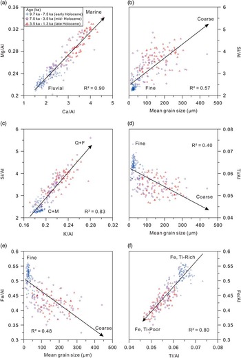
Though both river-suspended materials and eolian dust can contribute to the marine sediments (Bozzano et al., Reference Bozzano, Kuhlmann and Alonso2002; Plewa et al., Reference Plewa, Meggers, Kuhlmann, Freudenthal, Zabel and Kasten2012), eolian dust can be ignored because of the geographic location of core GeoB12605-3. Because the elemental ratios of Ca/Al, Mg/Al, and Sr/Al show good correlations to one another (Fig. 7a), we suggest that they share the same forcing and are mainly controlled by the fluvial discharge of the Pangani River. According to this interpretation, we infer that from the early to late Holocene, the fluvial discharge decreased (Fig. 7a).
(color online) Scatter plot between elemental ratios, classified by age. (a) Interaction between the elemental ratios of Ca/Al and Mg/Al, showing a decrease in fluvial discharge throughout the Holocene. (b) Si/Al ratio plotted as a function of the mean grain size of terrigenous sediments. (c) Interaction between the elemental ratios of K/Al and Si/Al. C+M, clay minerals and mica; Q+F, quartz and feldspar. (d, e) Ti/Al and Fe/Al ratios plotted as a function of the mean grain size of terrigenous sediments. (f) Scatter plot between Ti/Al and Fe/Al, indicating a shift in source area from the early to late Holocene.

Ratios between terrigenous elements and Al
The geochemical composition of terrigenous sediments may be affected by grain size (Bloemsma et al., Reference Bloemsma, Zabel, Stuut, Tjallingii, Collins and Weltje2012); thus, in response, terrigenous elemental ratios can be related to grain-size variations (Lupker et al., Reference Lupker, France-Lanord, Galy, Lavé and Kudrass2013). Among the terrigenous elements considered here, Si is associated with different minerals, spanning different grain size (e.g., fine-grained clay minerals and coarse-grained quartz; Just et al., Reference Just, Schefuss, Kuhlmann, Stuut and Pätzold2014). Al is mostly hosted in fine-grained clay minerals of terrigenous origin in marine sediments (Clift et al., Reference Clift, Wan and Blusztajn2014). Therefore, the ratio of Si/Al is indicative of grain size (Bouchez et al., Reference Bouchez, Gaillardet, France-Lanord, Maurice and Dutra-Maia2011; Bloemsma et al., Reference Bloemsma, Zabel, Stuut, Tjallingii, Collins and Weltje2012). As expected, a well-adjusted positive slope for the grain-size range and Si/Al ratio is obtained in Figure 7b (i.e., the coarser samples are Si enriched, whereas the finer samples are Al rich; thus Si/Al ratios increase when the sediments become coarser). In marine sediments, K derives from K-feldspar or illite, which are both characteristic of weak chemical weathering (Zabel et al., Reference Zabel, Schneider, Wagner, Adegbie, de Vries and Kolonic2001; Ziegler et al., Reference Ziegler, Simon, Hall, Barker, Stringer and Zahn2013); thus K/Al ratios have been used as an indicator for the intensity of chemical weathering in the source area. However, at the shelf off the Pangani River mouth, they display similar patterns to those observed in the Si/Al ratios, controlled by grain size (Fig. 7c). Clay minerals and mica (lower Si/Al and K/Al Al ratios) decrease from the early to late Holocene, whereas quartz and feldspar (higher Si/Al and K/Al ratios) contents increase continuously from the early to late Holocene (Liu et al., Reference Liu, Rendle-Bühring, Meyer and Henrich2016). Thus, an increase in Si/Al and K/Al ratios from the early to late Holocene is mainly controlled by the grain size of the terrigenous component, which shifted from fine- to coarse-grained sediments at the end of the early Holocene (Fig. 4b).
The Ti/Al ratio has been used as a grain-size proxy (Calvert and Pedersen, Reference Calvert and Pedersen2007) because Ti is carried in the silt and fine-sand fractions during transportation (i.e., Ti/Al increases when grain size becomes coarser). However, in core GeoB12605-3, a negative slope for the grain-size range and Ti/Al ratio is observed (i.e., decreasing ratios with increasing grain size; Fig. 7d). This inverse relationship is unexpected because Ti/Al ratios in other locations show positive correlations with grain size, which suggests that Ti/Al ratio might be controlled by other factors at our site. Ti concentrations in marine sediments may also change because of a shift in the source area (e.g., sediments derived from basaltic rocks are usually enriched in Ti; Plewa et al., Reference Plewa, Meggers, Kuhlmann, Freudenthal, Zabel and Kasten2012). A previous investigation on the Pangani River sediments indicates that the Ti concentration is higher in the upper stream region (Quaternary-Tertiary volcanic; Fig. 1b) than the lower region (Hellar-Kihampa et al., Reference Hellar-Kihampa, Potgieter-Vermaak, Van Meel, Rotondo, Kishimba and Van Grieken2012). Thus, the Ti/Al ratio of Tanzanian shelf sediments is plausibly interpreted to be controlled by a shift in the sediment source area, from the volcanic mountainous area to the coastal region and inner shelf. The Fe/Al ratio, similar to Ti/Al, also shows a negative correlation with grain size (Fig. 7e), indicating a strong genetic link with Ti/Al. Thus, the elemental ratios of Ti/Al and Fe/Al reflect the source of the terrigenous sediments during the Holocene (Fig. 7f), which reflect a shift that occurred at the end of the early Holocene (from Fe, Ti rich to Fe, Ti poor).
Geochemical variability in response to Holocene climatic and sea-level changes
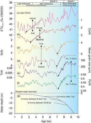
Numerous climatic records for the East African continental margin have shown that this region has experienced a transition from a humid early Holocene (AHP I), to a moderately humid early (AHP II) and late middle Holocene, and then an arid late Holocene (Liu et al., Reference Liu, Rendle-Bühring, Kuhlmann and Li2017; Fig. 8). Oceanographic records for this region, however, such as sea-level reconstructions are still rare (Zinke et al., Reference Zinke, Reijmer, Thomassin, Dullo, Grootes and Erlenkeuser2003; Camoin et al., Reference Camoin, Montaggioni and Braithwaite2004; Woodroffe et al., Reference Woodroffe, Long, Punwong, Selby, Bryant and Marchant2015). The limited records that do exist indicate that the early Holocene was a period of rapid sea-level rise off East Africa (Zinke et al., Reference Zinke, Reijmer, Thomassin, Dullo, Grootes and Erlenkeuser2003). Zinke et al. (Reference Zinke, Reijmer, Thomassin, Dullo, Grootes and Erlenkeuser2003) found that the sea-level rise had occurred at different rates since the onset of the last deglaciation and includes a fast sea-level rise during the early Holocene (19 mm/yr) between 11.6 and 9.6 ka, followed by a continuously rapid sea-level rise during the early middle Holocene, between 9.6 and 8 ka with a rate of 9 mm/yr, which fell to a rate of 3 mm/yr after 7 ka (Fig. 8g). These environmental influences have also played a role in the sediment pattern of the Tanzanian shelf system (autochthonous vs. allochthonous sedimentation; Liu et al., Reference Liu, Rendle-Bühring, Meyer and Henrich2016), which are fingerprinted in the geochemical composition of the marine sediments.
(color online) Comparison of geochemical and grain-size data with climatic and sea-level changes. (a) Lake Challa oxygen isotope values, based on Barker et al. (Reference Barker, Hurrell, Leng, Wolff, Cocquyt, Sloane and Verschuren2011), representing ratios of precipitation and evaporation, scale reversed. (b) Elemental ratios of Ca/Al from core GeoB12605-3, indicating the intensity of the fluvial discharge. (c, d) Si/Al ratios from core GeoB12605-3, comparing with the grain-size data. (e, f) Elemental ratios of Ti/Al and Fe/Al, indicating a shift in the sediment source area. (g) Composite sea-level curve off East Africa based on the data from the Mayotte foreslopes and the lagoon of Mayotte (Zinke et al., Reference Zinke, Reijmer, Thomassin, Dullo, Grootes and Erlenkeuser2003). EAHP, East African Humid Period. VSMOW, Vienna Standard Mean Ocean Water.

During the early Holocene (>7.5 ka), the higher rates in sea-level rise coincided with a phase when East Africa experienced a significantly humid period, the EAHP I (e.g., Lake Challa; Fig. 8a). At this time, enhanced precipitation in the hinterland would have resulted in intense erosion and an increase in fluvial discharge; thus elemental ratios of Ca/Al were low (Fig. 8b). The high Pangani River discharge, containing fine-grained suspended sediments (low Si/Al; Fig. 8c and d), caused the deposition of terrigenous-derived clay minerals and mica (enriched in Fe and Ti; Fig. 8e and f) on the shelf. Because of terrigenous sediment dilution, the Ca and Sr elements, coupled to the marine CaCO3 signal, were low when the sedimentation pattern was characterized by allochthonous sedimentation (Liu et al., Reference Liu, Rendle-Bühring, Meyer and Henrich2016). VSMOW, Vienna Standard Mean Ocean Water.
The early middle Holocene (7.5–5 ka) was influenced by the higher stand in sea level caused by the rapid rise during the early Holocene (Fig. 8g; Zinke et al., Reference Zinke, Reijmer, Thomassin, Dullo, Grootes and Erlenkeuser2003). During the EAHP II, the fluvial discharge would have decreased slightly as indicated by the fluctuations in the ratio of Ca/Al (Fig. 8b). An increase in grain size and the increase reflected in the Si/Al ratios (Fig. 8c and d) at this time suggest the idea of the correlation between the elemental ratio of Si/Al and grain size. This shift in grain size was caused by autochthonous sedimentation on the inner shelf of sediment composed of quartz and feldspar (Liu et al., Reference Liu, Rendle-Bühring, Meyer and Henrich2016).
A switch in source area would facilitate the coarser-grained sediment input. The source material of the coarse-grained material has lower Ti concentrations compared with the source material of the fine-grained sediments, reflecting a shift of the sediment source area (indicated by the arrows in Fig. 8e and f). We can therefore propose that the sediment source area changed from the upper drainage area (Fe, Ti rich; QTv in Fig. 1b) to the coast and inner shelf (Fe, Ti poor; QTMz in Fig. 1b) at the end of the early Holocene, which corresponds to our previous mineral record by Liu et al. (Reference Liu, Rendle-Bühring, Meyer and Henrich2016). This shift in the source area of the terrigenous sediments is the primary controlling factor for the elemental ratios of Ti/Al and Fe/Al observed at the research site during the transition from the early to mid-Holocene.
During the late middle Holocene (5–3.5 ka), when the climatic conditions transitioned from the EAHP climate regime to the arid climate of the late Holocene, the rate of sea-level rise was slowed, and sea level reached its present-day level (Woodroffe et al., Reference Woodroffe, Long, Punwong, Selby, Bryant and Marchant2015). Fine-grained fluvial terrigenous sediment input was low, as indicated by an increase in the Ca/Al ratio (Fig. 8b). The grain-size coarsening (deposition of very coarse sands) in the sediments at GeoB12605-3 suggests that reworked sediments were still being deposited (Fig. 8d). During the late Holocene, the climate became arid, and thus, the fluvial discharge was low, as represented by the low sedimentation rate (Fig. 2) and high Ca/Al ratios (Fig. 8b). Because of the reduction of deposited fine-grained sediments and coast erosion, grain size became coarser, as represented by an increase in the elemental ratios of Si/Al (Fig. 8c and d).
Implications for the termination of the EAHP
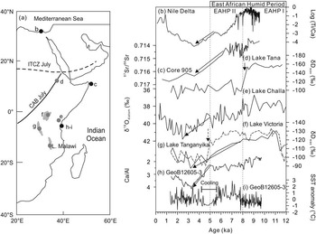
Based on the existing records (Fig. 9), the pace of the termination of the EAHP is still controversial. According to the elemental ratios of Ti/Ca, Blanchet et al. (Reference Blanchet, Tjallingii, Frank, Lorenzen, Reitz, Brown, Feseker and Brückmann2013) suggested that the terrigenous sediments discharged by the Nile River decreased gradually from 7.3 to 3 ka (Fig. 9b). A strontium isotopic record off northeast Africa shows that aridification began at 6 ka and ceased at 3.8 ka (Jung et al., Reference Jung, Davies, Ganssen and Kroon2004; Fig. 9c). Isotopic records from Lakes Challa (Barker et al., Reference Barker, Hurrell, Leng, Wolff, Cocquyt, Sloane and Verschuren2011) and Victoria (Berke et al., Reference Berke, Johnson, Werne, Grice, Schouten and Damste2012) also demonstrated a gradual transition from the humid early Holocene to the arid late Holocene (Fig. 9e and f). In contrast, δD at Lake Tanganyika (Fig. 9g), as a signal for the amount of precipitation, suggests an abrupt termination of the EAHP around 5 ka (Tierney et al., Reference Tierney, Russell, Huang, Damste, Hopmans and Cohen2008); however, this signal has also been influenced by the moisture source (Costa et al., Reference Costa, Russell, Konecky and Lamb2014), which has been documented in Lake Tana (Fig. 9b). Other records, such as the lake levels in this region, also show inconsistency in both timing and abruptness of the EAHP (e.g., Garcin et al., Reference Garcin, Melnick, Strecker, Olago and Tiercelin2012; Junginger et al., Reference Junginger, Roller, Olaka and Trauth2014; Morrissey and Scholz, Reference Morrissey and Scholz2014). These spatial and temporal patterns have been related to shifts in the mean position of the ITCZ and CAB, as well as the influence of the sea-surface temperatures (SSTs) of the Atlantic and Indian Oceans (Tierney et al., Reference Tierney, Russell, Damste, Huang and Verschuren2011b).
(a) Comparison of paleoclimatic records around East Africa. (b) Ti/Ca ratios from a sediment core off the Nile Delta, representing terrigenous versus marine sedimentation (Blanchet et al., Reference Blanchet, Tjallingii, Frank, Lorenzen, Reitz, Brown, Feseker and Brückmann2013). (c) Sr isotope ratios of the dust fraction off Somalia (core 905), reflecting the precipitation/evaporation balance (Jung et al., Reference Jung, Davies, Ganssen and Kroon2004). (d) δD of leaf wax for Lake Tana, indicating the precipitation amount (Costa et al., Reference Costa, Russell, Konecky and Lamb2014). (e) Oxygen isotope diatom record for Lake Challa, representing ratios of precipitation and evaporation (Barker et al., Reference Barker, Hurrell, Leng, Wolff, Cocquyt, Sloane and Verschuren2011). (f, g) δD of leaf wax at Lake Victoria (solid line; Berke et al., Reference Berke, Johnson, Werne, Grice, Schouten and Damste2012) and Lake Tanganyika (dashed line; Tierney et al., Reference Tierney, Russell, Huang, Damste, Hopmans and Cohen2008), indicating the precipitation amount. (h) Ca/Al ratios from core GeoB12605-3 off Tanzania, representing marine versus terrigenous sedimentation, this study. (i) Sea-surface temperature (SST) anomalies from core GeoB12605-3 based on Mg/Ca ratios of Globigerinoides ruber (Kuhnert et al., Reference Kuhnert, Kuhlmann, Mohtadi, Meggers, Baumann and Pätzold2014). CAB, Congo Air Boundary; ITCZ, Intertropical Convergence Zone.

Our high-resolution geochemical results show that ratios of Ca/Al from core GeoB12605-3 correlate closely with fluctuations in the oxygen isotopes extracted from diatom silica in Lake Challa sediments (Fig. 9e and h), which have been used to indicate the ratios between local precipitation and evaporation by Barker et al. (Reference Barker, Hurrell, Leng, Wolff, Cocquyt, Sloane and Verschuren2011). This suggests that elemental ratios of Ca/Al are sensitive to fluvial discharge and can reflect fluctuations of precipitation in the hinterland when the sea level of the WIO became stabilized during the mid- and late Holocene. These high-resolution elemental ratios (i.e., Ca/Al, Sr/Al, and Mg/Al) thus could be regarded as potential indicators to study the termination of the EAHP. An increase in ratios of Ca/Al occurred at 5–3.5 ka, coupled with an increase in oxygen isotopes (Fig. 9e and h), indicating that the termination of the EAHP in this study region might have been gradual. Furthermore, some previous X-ray fluorescence (XRF) data sets also support this conclusion, such as a gradual decrease in the ratios of Fe (Ti) Ca of marine sediment cores from the Mediterranean Sea (Blanchet et al., Reference Blanchet, Tjallingii, Frank, Lorenzen, Reitz, Brown, Feseker and Brückmann2013; Revel et al., Reference Revel, Colin, Bernasconi, Combourieu-Nebout, Ducassou, Grousset and Rolland2014; Castañeda et al., Reference Castañeda, Schouten, Pätzold, Lucassen, Kasemann, Kuhlmann and Schefuß2016; Figs. 2c and 9b). An apparently abrupt termination of the EAHP, as indicated by a rapid increase in a δDwax record, could reflect a shift in the dominant moisture source rather than rainfall amount effect, which has been suggested recently by Costa et al. (Reference Costa, Russell, Konecky and Lamb2014) and Castañeda et al. (Reference Castañeda, Schouten, Pätzold, Lucassen, Kasemann, Kuhlmann and Schefuß2016).
The termination of the EAHP reflected by our high-resolution geochemical profile corresponds to a decrease in the SST record derived from the same sediment core (Kuhnert et al., Reference Kuhnert, Kuhlmann, Mohtadi, Meggers, Baumann and Pätzold2014; Fig. 9i). This relation between the increase in the elemental ratios of Ca/Al and the mid-Holocene cooling interval (5.6–4.2 ka) might have been caused by increasing carbonate production because of the cooling SST. However, taking into account the low productivity in the research area (Liu et al., Reference Liu, Rendle-Bühring, Kuhlmann and Li2017), the most likely cause is that cooling waters in the WIO resulted in a decrease in inland precipitation, which, in turn, reduced the terrigenous discharge of the Pangani River. SST anomalies in the WIO have been proposed as possible drivers for Holocene climate variability in the hinterland of East Africa (Tierney and deMenocal, Reference Tierney and deMenocal2013). Therefore, our new data sets suggest that the termination of the EAHP in this research region likely has been gradual and responding to the decrease in the SST of the adjacent ocean.
CONCLUSIONS
We present a high-resolution geochemical record off Tanzania, with average temporal resolution ~40 yr, to estimate the sediment sources into the WIO and their implications for climatic and sea-level changes during the Holocene. Among the ratios between terrigenous elements and Al, the ratios Si/Al and K/Al provide reasonable proxies for grain size in the region off the Tanzanian margin, whereas the ratios of Ti/Al and Fe/Al show a negative correlation to the grain size of the terrigenous sediments, which is unexpected. We propose that elemental ratios of Ti/Al and Fe/Al reflect the source area of the terrigenous sediments during the Holocene. These elemental ratios demonstrate a shift in the source area that occurred at the end of the early Holocene (from Fe, Ti rich to Fe, Ti poor) in response to Holocene climatic and sea-level changes. Elemental ratios between biogenic elements and Al (i.e., Ca/Al, Mg/Al, and Sr/Al) are mainly controlled by the fluvial discharge of the Pangani River. Further, our geochemical results imply that elemental ratios could serve as potential indicators for precipitation in the hinterland of East Africa when the sea level was stabilized at the end of the early Holocene. Our results infer that the termination of the EAHP might have been gradual at this study area, indicating that the end of the AHP in East Africa might have been related to the cooler SST in the WIO. Further high-resolution marine records off East Africa are needed to discover the back-driven forcing for aridification of East Africa.
ACKNOWLEDGMENTS
We acknowledge three anonymous reviewers for their thoughtful and constructive comments that improved the manuscript, and the associate editor, Matthew Lachniet, for his valuable comments. We thank the crew and scientists of R/V Meteor Cruise M75/2 for collecting the gravity core. We are also grateful to Dr. Matthias Zabel (University of Bremen) and Dr. Inka Meyer (Ghent University) for XRF and grain-size measurements, respectively. Financial support for this study was provided by the DFG (Deutsche Forschungsgemeinschaft) Research Center/Cluster of Excellence “The Ocean in the Earth System.” XL was supported by the National Natural Science Foundation of China (grant nos. 41606062 and 41430965) and the China Postdoctoral Science Foundation (grant no. 2016M592257).