





1 Introduction
The study of two phase systems is both of practical significance in engineering and fundamental interest in the pure sciences. For example, continued miniaturisation of mechanical and electrical components has led to steep increases in power density, making thermal management a critical aspect of microelectronics and microelectromechanical systems (MEMS) design today. Evaporation and condensation are very efficient modes of heat transfer and as such are employed in component cooling and in energy conversion systems (Ling et al. Reference Ling, Zhang, Shi, Fang, Wang, Gao, Fang, Xu, Wang and Liu2014; Plawsky et al. Reference Plawsky, Fedorov, Garimella, Ma, Maroo, Chen and Nam2014) leading to considerable research into the study of phase transition at the micro and nano scales. Understanding the evaporation of liquid droplets is critical to a broad range of natural processes, such as body temperature control of mammals (Sherwood Reference Sherwood2005), and many industrial cooling processes, such as spray drying, spray cooling and microelectronics cooling (Dhavaleswarapu, Murthy & Garimella Reference Dhavaleswarapu, Murthy and Garimella2012; Plawsky et al. Reference Plawsky, Fedorov, Garimella, Ma, Maroo, Chen and Nam2014; Hodes et al. Reference Hodes, Steigerwalt, Shi, Cowley, Enright and MacLachlan2015).
One of the main difficulties in the description of phase-change microflows is that the classical Navier–Stokes–Fourier (NSF) model can fail to accurately capture the vapour flow. The breakdown of the NSF model can be quantified by the Knudsen number,
 $Kn=\unicode[STIX]{x1D706}/L$
, which is defined as the ratio of the molecular mean free path
 $\unicode[STIX]{x1D706}$
to the macroscopic length scale
 $L$
. The classical description of the NSF equations is applicable only when the Knudsen number is sufficiently small
 $(Kn\lesssim 10^{-1})$
; also known as the continuum and slip flow regime. In the opposite limiting case,
 $Kn\gtrsim 10$
, the mean free path is large as compared to the macroscopic dimensions of the system; this is known as the free molecular flow regime. The intermediate range between these extremes is the transitional regime (
 $10^{-1}\lesssim Kn\lesssim 10$
).
Many interesting rarefaction effects are observed in the transitional regime, such as velocity slip and temperature jump at boundaries, Knudsen layers, transpiration flow, thermal stress and heat flux without temperature gradients (Sone Reference Sone2007; Struchtrup & Torrilhon Reference Struchtrup and Torrilhon2008; Gu, Emerson & Tang Reference Gu, Emerson and Tang2010; Rana, Torrilhon & Struchtrup Reference Rana, Torrilhon and Struchtrup2013); these non-equilibrium effects cannot be described by the classical NSF equations and associated boundary conditions. This means that although the liquid phase is often accurately captured by the NSF equations, since the considered length scales are well above the molecular dimensions in the liquid, the properties of vapour in the vicinity of the liquid–vapour interface need to be modelled with more accurate transport models.
At sufficiently low temperatures, the saturated vapour can be treated as an ideal gas, which is well described by the Boltzmann equation, an evolution equation for the distribution function of the gas particles (Cercignani Reference Cercignani1975). The Boltzmann equation involves detailed information of phase space and thus its direct solution typically requires considerable computational resources. Often, it is solved by utilising the direct simulation Monte Carlo (DSMC) method (Bird Reference Bird1994). However, this is computationally expensive, particularly for the low-speed, moderate Knudsen number flows encountered in micro/nano devices.
When the perturbation of the distribution function from the equilibrium state is assumed small, the Boltzmann equation can be simplified through linearisation. Further simplification can be obtained when the Boltzmann collision operator is approximated by simplified collision models; such as the Bhatnagar–Gross–Krook (BGK) model (Bhatnagar, Gross & Krook Reference Bhatnagar, Gross and Krook1954), the ellipsoidal statistical BGK (ES-BGK) model and the S-model (Sharipov & Seleznev Reference Sharipov and Seleznev1998). Applications of these methods to the droplet evaporation process are reported in the literature; see e.g. Chernyak & Margilevskiy (Reference Chernyak and Margilevskiy1989), Takata et al. (Reference Takata, Sone, Lhuilliere and Wakabayashi1998) and Sone (Reference Sone2007). However, in all these simplified models the phase space still needs to be resolved, making them in many cases prohibitively computationally expensive.
Besides the Boltzmann equation, rarefaction effects that are beyond the resolution of the NSF system can be predicted by extended macroscopic moment equations (Struchtrup Reference Struchtrup2005; Struchtrup & Torrilhon Reference Struchtrup and Torrilhon2008; Gu & Emerson Reference Gu and Emerson2009), which were the subject of a recent article in the Annual Review of Fluid Mechanics (Torrilhon Reference Torrilhon2016). The moment equations form a set of partial differential equations describing the evolution of macroscopic quantities, such as mass density, temperature, velocity, heat flux, stress tensor and so on, defined as moments of the distribution function. These equations are obtained by an asymptotic reduction of the Boltzmann equation at different levels of approximation. The moment method was introduced to gas kinetic theory by Grad (Reference Grad1949), who expressed the distribution function in terms of Hermite polynomials. More recently, the regularisation of Grad’s 13-moment (G13) equations have been obtained by Struchtrup & Torrilhon (Reference Struchtrup and Torrilhon2003). The regularised 13-moment (R13) equations introduce additional terms to the G13 equations that overcome various deficiencies, such as the prediction of sub-shocks at high Mach number (
 $Ma\gtrsim 1.65$
). Gu & Emerson (Reference Gu and Emerson2007) presented a set of wall boundary conditions for the R13 equations derived from the Maxwell accommodation model. However, in their work unphysical oscillations were reported near the boundary due to the over-prescription of the boundary conditions, as identified and rectified by Torrilhon & Struchtrup (Reference Torrilhon and Struchtrup2008). Thus far, the R13 equations have been considered for canonical boundary-value problems, such as planar and cylindrical Couette and Poiseuille flows (Taheri et al.
Reference Taheri, Rana, Torrilhon and Struchtrup2009; Taheri & Struchtrup Reference Taheri and Struchtrup2009), transpiration flows and gas flow past a sphere (Torrilhon Reference Torrilhon2010), among others, in one- and two-dimensional numerical simulations.
To extend the applicability of the moment method further into the transition regime, Gu & Emerson (Reference Gu and Emerson2009) used the regularisation process to obtain the regularised 26-moment (R26) equations. The kinetic wall boundary conditions for the R26 equations were also derived in the same paper using the Maxwell accommodation model. The R26 theory describes Knudsen layers (regions of strongly non-equilibrium behaviour within a few mean free paths of the boundary) more accurately than the R13 equations (Gu & Emerson Reference Gu and Emerson2014); the NSF and G13 equations are not able to predict these at all. The R13/R26 systems have produced accurate results for small to moderate
 $Kn$
and have the advantage that they offer fast, sometimes analytic, solutions to enable us to understand, and develop intuition for the general flow behaviour. In this article, we shall consider whether similar results can be derived for phase-change phenomena.
1.1 Modelling evaporation and condensation
Flows involving evaporation/condensation processes are usually modelled using a sharp interface approach, where the interface separating the vapour and liquid phases is assumed to be infinitely thin. The phase transition process itself is modelled by setting the appropriate boundary conditions on the interface. Different variants of these boundary conditions have been employed in the literature. The standard assumptions, found in numerous classical textbooks and incorporated into most computational fluid dynamics software, is that the temperature and the velocity tangential to the interface are continuous across it. However, it is now well established, both experimentally and theoretically, that such assumptions are invalid at small length scales, where a velocity slip and temperature jump are observed (McGaughey & Ward Reference McGaughey and Ward2002; Rahimi & Ward Reference Rahimi and Ward2005).
The first mathematical model for the evaporation and condensation processes was developed by Maxwell (Reference Maxwell1867) for quasi-steady flow, where the flow at the interface can be assumed equal to the diffusion vapour flow far away from the interface. However, the classical diffusion flow of vapour starts beyond the Knudsen layer. The Hertz–Knudsen–Schrage (HKS) relation (Schrage Reference Schrage1953) can be applied to model the mass flux across the interface, along with the NSF equations in the bulk, provided
 $Kn$
is sufficiently small (Persad & Ward Reference Persad and Ward2016). Fuchs (Reference Fuchs1959) obtained a semi-empirical formula to account for the Knudsen layer by matching the free molecular solution, valid at the interface, with the diffusion solution valid at the edge of the Knudsen layer, the width of which is used as a fitting parameter to give a good match for all
 $Kn$
. Young (Reference Young1991) furthered this approach by deriving expressions for the mass and energy fluxes across a fluid droplet in a pure vapour assuming the G13 distribution inside the Knudsen layer. However, Young’s approach also involves an empirical parameter (related to thickness of the Knudsen layer) and does not resolve the Knudsen layer properly.
Bond & Struchtrup (Reference Bond and Struchtrup2004) considered interface conditions using the kinetic theory of gases and irreversible thermodynamics (using NSF equations) to develop predictive expressions for the mass and energy fluxes across the interface and compared the results between irreversible thermodynamics, statistical rate theory and experimental data. In particular, they considered a condensation coefficient which depends on the impact energy of the condensing particle and also pointed out the effect of interfacial curvature on temperature jump. More recently, steps towards using higher-order moment methods for mass and energy transport across the phase boundary were made by Struchtrup & Frezzotti (Reference Struchtrup and Frezzotti2016), with a full set of boundary conditions for the R13 equations derived and solved for a planar case. In this article, we extend this work to both curved interfaces, using spherical drops, and also derive phase-change boundary conditions for the R26 moment equations. This will allow us to compare the NSF, R13 and R26 models for evaporation and condensation for both a spherical droplet and a planar interface, in order to establish their accuracy against benchmark solutions from the Boltzmann equation. In this article, due to the linearity of the equations and boundary conditions considered, the results obtained for the evaporation process can simply be translated to condensation by reversing the signs of thermodynamics forces.
The article is organised as follows. A brief summary of basic elements of kinetic theory and the moment method is given in § 2, followed by the derivation of moment equations, namely the NSF, R13 and R26 equations for a spherical geometry, in § 3. In § 4, analytical solutions to these equations are found. In § 5, boundary conditions for the R26 equations are derived and applied for the evaporation problem. Throughout §§6–8, Boltzmann solutions provide the benchmark for our analytic results; beginning, in § 6, by considering
 $Kn\rightarrow 0$
. In § 9, we analyse the magnitude of competing higher-order contributions to the total normal stress. Finally, in § 10 we conclude and discuss future directions of research.
2 Moment methods in kinetic theory
Sufficiently far from the critical point, the vapour can be treated as an ideal gas and one can use the kinetic theory of dilute gases for this phase. A monoatomic ideal gas can be characterised by a one-particle distribution function
 $f$
which depends on time
 $t$
, spatial coordinates
 $x_{i}$
and molecular velocity
 $~c_{i}$
. The distribution function is governed by the Boltzmann equation (Kogan Reference Kogan1969; Cercignani Reference Cercignani1975)
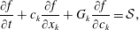 $$\begin{eqnarray}\frac{\unicode[STIX]{x2202}f}{\unicode[STIX]{x2202}t}+c_{k}\frac{\unicode[STIX]{x2202}f}{\unicode[STIX]{x2202}x_{k}}+G_{k}\frac{\unicode[STIX]{x2202}f}{\unicode[STIX]{x2202}c_{k}}={\mathcal{S}},\end{eqnarray}$$
where
 $G_{k}$
is the external force per unit mass acting on the gas and is assumed to be independent of the microscopic velocity
 $c_{k}$
. The term
 ${\mathcal{S}}$
is the collision operator that describes the change of the distribution function due to interaction between particles.
For most engineering processes, the main interest is not in detailed information about the distribution function
 $f$
, but in the macroscopic quantities, such as mass density
 $\unicode[STIX]{x1D71A}$
, macroscopic velocity
 $v_{i}$
, and temperature
 $T$
. These are defined as moments of the distribution function:
 $$\begin{eqnarray}\displaystyle & \displaystyle \unicode[STIX]{x1D71A}=\int f\,\mathbf{d}\boldsymbol{c}, & \displaystyle\end{eqnarray}$$
 $$\begin{eqnarray}\displaystyle & \displaystyle v_{i}=\frac{1}{\unicode[STIX]{x1D71A}}\int c_{i}f\,\mathbf{d}\boldsymbol{c}, & \displaystyle\end{eqnarray}$$
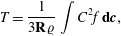 $$\begin{eqnarray}\displaystyle & \displaystyle T=\frac{1}{3\mathbf{R}\unicode[STIX]{x1D71A}}\int C^{2}f\,\mathbf{d}\boldsymbol{c}, & \displaystyle\end{eqnarray}$$
where
 $C_{i}=c_{i}-v_{i}$
is the peculiar velocity,
 $\text{R}$
is the gas constant and
 $\mathbf{d}\boldsymbol{c}=dc_{1}\,dc_{2}\,dc_{3}$
. The temperature is related to the pressure
 ${\wp}$
and density by the ideal-gas law
 ${\wp}=\unicode[STIX]{x1D71A}RT$
. The pressure tensor
 $\unicode[STIX]{x1D631}_{ij}$
, and the heat-flux vector
 $q_{i}$
are the second and contracted third-order moments of the distribution function
 $f$
, respectively, i.e.
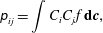 $$\begin{eqnarray}\displaystyle & \displaystyle \unicode[STIX]{x1D631}_{ij}=\int C_{i}C_{j}f\,\mathbf{d}\boldsymbol{c}, & \displaystyle\end{eqnarray}$$
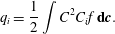 $$\begin{eqnarray}\displaystyle & \displaystyle q_{i}=\frac{1}{2}\int C^{2}C_{i}f\,\mathbf{d}\boldsymbol{c}. & \displaystyle\end{eqnarray}$$
Furthermore, the pressure tensor can be separated as
 $\unicode[STIX]{x1D631}_{ij}={\wp}\unicode[STIX]{x1D6FF}_{ij}+\unicode[STIX]{x1D70E}_{ij}$
, where
 $\unicode[STIX]{x1D6FF}_{ij}$
is the Kronecker delta,
 $\unicode[STIX]{x1D70E}_{ij}=\unicode[STIX]{x1D631}_{\langle ij\rangle }$
is the deviatoric stress tensor, and
 ${\wp}=p_{kk}/3$
is the pressure. The angular brackets are used to denote the traceless part of a symmetric tensor.
Instead of attempting a direct solution of the Boltzmann equation (2.1), the moment method provides a bridge between kinetic theory and classical hydrodynamics via evolution equations, known as moment equations, for the macroscopic moments. A set of moment equations is obtained by multiplication of the Boltzmann equation (2.1) with an arbitrary function
 $\unicode[STIX]{x1D6F9}_{A}$
and subsequent integration over the microscopic velocity space. For example, by choosing
 $\unicode[STIX]{x1D6F9}_{A}=1$
,
 $c_{i}$
and
 $C^{2}/2$
, we get the conservation laws for mass, momentum and energy densities, respectively. However, in pronounced non-equilibrium situations, it is necessary to extend the set of macroscopic variables beyond the 5 conservative variables, so as to include higher-order moments. For instance, in the 13-moment approximation
 $\unicode[STIX]{x1D6F9}_{A}=1$
,
 $c_{i}$
,
 $C_{i}C_{j}$
and
 $C^{2}C_{i}/2$
, corresponding to the 13 moments (
 $5$
conservative variables,
 $5$
components of
 $\unicode[STIX]{x1D70E}_{ij}$
and
 $3$
components of
 $q_{i}$
). A further extension of the moment equations contain even higher-order moments (see below) and here we follow the same notation as used in Gu & Emerson (Reference Gu and Emerson2009) for the R26 equations, where
 $\unicode[STIX]{x1D6E5}$
,
 $\unicode[STIX]{x1D6FA}_{i}$
,
 $\unicode[STIX]{x1D619}_{ij}$
,
 $\unicode[STIX]{x1D62E}_{ijk}$
,
 $\unicode[STIX]{x1D713}_{ijk}$
and
 $\unicode[STIX]{x1D719}_{ijkl}$
are scalar, first-, second-, third- and fourth-order symmetric trace-free tensors, respectively, defined as
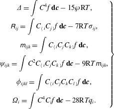 $$\begin{eqnarray}\left.\begin{array}{@{}c@{}}\displaystyle \unicode[STIX]{x1D6E5}=\int C^{4}f\,\mathbf{d}\boldsymbol{c}-15{\wp}\text{R}T,\\ \displaystyle \unicode[STIX]{x1D619}_{ij}=\int C_{\langle i}C_{j\rangle }f\,\mathbf{d}\boldsymbol{c}-7\text{R}T\unicode[STIX]{x1D70E}_{ij},\\ \displaystyle \unicode[STIX]{x1D62E}_{ijk}=\int C_{\langle i}C_{j}C_{k\rangle }f\,\mathbf{d}\boldsymbol{c},\\ \displaystyle \unicode[STIX]{x1D713}_{ijk}=\int C^{2}C_{\langle i}C_{j}C_{k\rangle }f\,\mathbf{d}\boldsymbol{c}-9\text{R}T\unicode[STIX]{x1D62E}_{ijk},\\ \displaystyle \unicode[STIX]{x1D719}_{ijkl}=\int C_{\langle i}C_{j}C_{k}C_{l\rangle }f\,\mathbf{d}\boldsymbol{c},\\ \displaystyle \unicode[STIX]{x1D6FA}_{i}=\int C^{4}C_{i}f\,\mathbf{d}\boldsymbol{c}-28\text{R}Tq_{i}.\end{array}\right\}\end{eqnarray}$$
Here, the higher moments have been constructed in such a way that they vanish in the 13-moment theory. The governing equations for the moments can be readily obtained from the Boltzmann equation (2.1), see e.g. Struchtrup (Reference Struchtrup2005); however, they cannot be solved as they stand, since they do not form a closed set of equations. The regularisation process presented by Struchtrup & Torrilhon (Reference Struchtrup and Torrilhon2003) and Struchtrup (Reference Struchtrup2004) provides a framework to derive a closed set of moment equations, giving the R13 equations at third-order accuracy while at the fifth order we arrive at the R26 equations, see Struchtrup (Reference Struchtrup2005) and Gu & Emerson (Reference Gu and Emerson2009). The derivation of the R13 and R26 moment equations for a monatomic gas of Maxwell molecules (i.e. molecules repelling each other with an intermolecular force
 $\propto r^{-5}$
) and their linearised version can be found in Taheri & Struchtrup (Reference Taheri and Struchtrup2009), Gu et al. (Reference Gu, Emerson and Tang2010) and Gu & Emerson (Reference Gu and Emerson2014). The equations of these models will now be presented for the spherically symmetric case.
2.1 Problem statement
Consider a liquid droplet of fixed radius
 $R_{0}$
at a given temperature
 $T_{l}$
, with corresponding saturation pressure in the liquid
 ${\wp}_{l}$
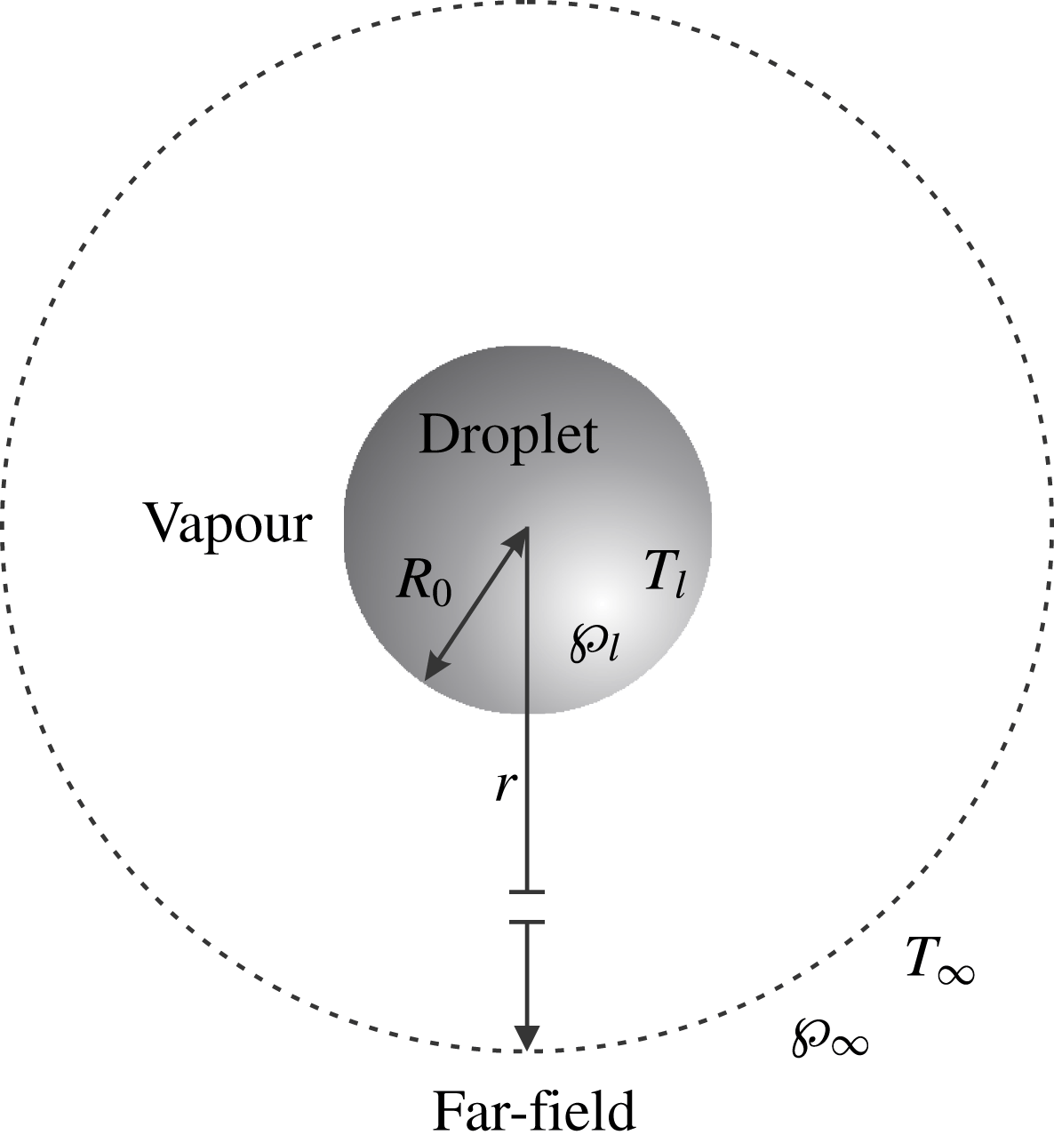
, immersed in its own vapour; see figure 1. This problem has been studied fairly extensively, e.g. Sone & Onishi (Reference Sone and Onishi1978), Chernyak & Margilevskiy (Reference Chernyak and Margilevskiy1989), Takata et al. (Reference Takata, Sone, Lhuilliere and Wakabayashi1998), which allows us to test the accuracy of the derived evaporation/condensation boundary conditions for the extended moment equations. Let the temperature and pressure of the vapour at a distance far from the surface of the droplet be given by
 $T_{\infty }$
and
 ${\wp}_{\infty }$
, respectively. In general, the saturation pressure
 ${\wp}_{l}$
is a function of
 $T_{l}$
given by the Clausius–Clapeyron relation; however, when the droplet has fixed properties this is not invoked so that
 ${\wp}_{l}$
and
 $T_{l}$
can be varied independently.
A spherical coordinate system (
 $r$
,
 $\unicode[STIX]{x1D703}$
,
 $\unicode[STIX]{x1D711}$
) is considered, and because of the spherical symmetry, the flow is independent of the azimuthal and polar directions. Two cases will be considered.
Schematic representation of a liquid droplet surrounded by its own vapour.
 $T_{l}$
is the temperature of liquid at the interface which corresponds to the saturation pressure
 ${\wp}_{l}$
. The temperature and pressure of the vapour at distance far from the surface of the droplet are given as
 $T_{\infty }$
and
 ${\wp}_{\infty }$
, respectively.
-
(i) Pressure-driven flow. The process in the vapour is driven by a dimensionless pressure difference
 $p_{l}=({\wp}_{l}-{\wp}_{\infty })/{\wp}_{\infty }$
while the temperature of the liquid is equal to the far-field temperature.
-
(ii) Temperature-driven flow. The process is driven by a dimensionless temperature difference
$\unicode[STIX]{x1D703}_{l}=(T_{l}-T_{\infty })/T_{\infty }$
while the saturation pressure in the liquid is same as the far-field pressure.


In general, any combination of these two cases can be superimposed, owing to the linearity of the equations and boundary conditions considered.
As a result of the flow configuration, the velocity vector
 $\boldsymbol{v}$
, the heat-flux vector
 $\boldsymbol{q}$
and stress tensor
 $\unicode[STIX]{x1D748}$
simplify to
 $$\begin{eqnarray}\boldsymbol{v}\equiv \left\{v(r),~0,0\right\},\quad \boldsymbol{q}\equiv \left\{q(r),0,0\right\}\quad \text{and}\quad \unicode[STIX]{x1D748}\equiv \left\{\begin{array}{@{}ccc@{}}\unicode[STIX]{x1D70E}(r) & 0 & 0\\ 0 & -\displaystyle \frac{\unicode[STIX]{x1D70E}(r)}{2} & 0\\ 0 & 0 & -\displaystyle \frac{\unicode[STIX]{x1D70E}(r)}{2}\end{array}\right\}.\end{eqnarray}$$
Furthermore, the only non-zero components of the higher-order tensors
 $\unicode[STIX]{x1D6FA}_{i}$
,
 $\unicode[STIX]{x1D619}_{ij}$
,
 $\unicode[STIX]{x1D62E}_{ijk}$
,
 $\unicode[STIX]{x1D713}_{ijk}$
and
 $\unicode[STIX]{x1D719}_{ijkl}$
are
 $$\begin{eqnarray}\displaystyle & \displaystyle \unicode[STIX]{x1D6FA}_{r}\equiv \unicode[STIX]{x1D714}(r), & \displaystyle\end{eqnarray}$$
 $$\begin{eqnarray}\displaystyle & \displaystyle \unicode[STIX]{x1D619}_{rr}=-2\unicode[STIX]{x1D619}_{\unicode[STIX]{x1D711}\unicode[STIX]{x1D711}}=-2\unicode[STIX]{x1D619}_{\unicode[STIX]{x1D703}\unicode[STIX]{x1D703}}\equiv R(r), & \displaystyle\end{eqnarray}$$
 $$\begin{eqnarray}\displaystyle & \displaystyle \unicode[STIX]{x1D62E}_{rrr}=-2\unicode[STIX]{x1D62E}_{r\unicode[STIX]{x1D711}\unicode[STIX]{x1D711}}=-2\unicode[STIX]{x1D62E}_{r\unicode[STIX]{x1D703}\unicode[STIX]{x1D703}}\equiv m(r), & \displaystyle\end{eqnarray}$$
 $$\begin{eqnarray}\displaystyle & \displaystyle \unicode[STIX]{x1D713}_{rrr}=-2\unicode[STIX]{x1D713}_{r\unicode[STIX]{x1D711}\unicode[STIX]{x1D711}}=-2\unicode[STIX]{x1D713}_{r\unicode[STIX]{x1D703}\unicode[STIX]{x1D703}}\equiv \unicode[STIX]{x1D713}(r), & \displaystyle\end{eqnarray}$$
 $$\begin{eqnarray}\displaystyle & \displaystyle \unicode[STIX]{x1D719}_{rrrr}=-2\unicode[STIX]{x1D719}_{rr\unicode[STIX]{x1D711}\unicode[STIX]{x1D711}}=-2\unicode[STIX]{x1D719}_{rr\unicode[STIX]{x1D703}\unicode[STIX]{x1D703}}={\textstyle \frac{8}{3}}\unicode[STIX]{x1D719}_{\unicode[STIX]{x1D703}\unicode[STIX]{x1D703}\unicode[STIX]{x1D703}\unicode[STIX]{x1D703}}={\textstyle \frac{8}{3}}\unicode[STIX]{x1D719}_{\unicode[STIX]{x1D711}\unicode[STIX]{x1D711}\unicode[STIX]{x1D711}\unicode[STIX]{x1D711}}\equiv \unicode[STIX]{x1D6F7}(r), & \displaystyle\end{eqnarray}$$
2.2 Relation to the unsteady evaporation of a drop
The steady process considered in this article will form the basis of future work into the unsteady problem, where one is interested in how long it takes a drop to completely evaporate. In this case, the temperature distribution inside the liquid drop
 $T_{l}(t,r)$
must be calculated as part of the solution, as must the position of the drop’s radius
 $R(t)$
, see e.g. the molecular dynamics study by Holyst & Litniewski (Reference Hołyst and Litniewski2008) and the experimental and theoretical study by Holyst et al. (Reference Hoyst, Litniewski, Jakubczyk, Kolwas, Kolwas, Kowalski, Migacz, Palesa and Zientara2013). The pressure inside the liquid is also now part of the solution with the saturation pressure
 ${\wp}_{l}$
a function of
 $T_{l}$
and
 $R$
given by the Clausius–Clapeyron relation with corrections (Kelvin equation) that account for the curvature of the liquid–vapour interface (Young Reference Young1991). The problem can be significantly simplified owing to the high density ratio between the liquid and the vapour phase, which creates a quasi-steady process in the vapour phase.
To determine the radius of the drop and the temperature distribution in the liquid the mass flux
 $j$
and heat flux
 $q$
into the vapour must be calculated. For small deviations from equilibrium, i.e.
 $p_{l}\ll 1$
and
 $\unicode[STIX]{x1D703}_{l}\ll 1$
, the pressure-driven and temperature-driven cases can be combined to give the mass flux
 $j$
and the heat flux
 $q$
as
 $$\begin{eqnarray}\displaystyle & \displaystyle j=j^{p}p_{l}+j^{\unicode[STIX]{x1D70F}}\unicode[STIX]{x1D703}_{l}, & \displaystyle\end{eqnarray}$$
 $$\begin{eqnarray}\displaystyle & \displaystyle q=q^{p}p_{l}+q^{\unicode[STIX]{x1D70F}}\unicode[STIX]{x1D703}_{l}, & \displaystyle\end{eqnarray}$$
where,
 $j^{p}(q^{p})$
and
 $j^{\unicode[STIX]{x1D70F}}(q^{\unicode[STIX]{x1D70F}})$
are the mass (heat) flux for the pressure-driven and the temperature-driven cases, respectively, and are derived in this article.
3 Extended moment equations in spherical geometry
Let
 $R_{0}$
,
 ${\wp}_{\infty }$
,
 $T_{\infty }$
be the reference length, pressure and temperature, respectively. The equations are made dimensionless by introducing
 $$\begin{eqnarray}\displaystyle & \displaystyle \hat{\unicode[STIX]{x1D703}}=\frac{T-T_{\infty }}{T_{\infty }},\quad \hat{p}=\frac{{\wp}-{\wp}_{\infty }}{{\wp}_{\infty }},\quad \hat{\unicode[STIX]{x1D70E}}=\frac{\unicode[STIX]{x1D70E}}{{\wp}_{\infty }},\quad \hat{v}=\frac{v}{\sqrt{\text{R}T_{\infty }}}, & \displaystyle\end{eqnarray}$$
 $$\begin{eqnarray}\displaystyle & \displaystyle \hat{q}=\frac{q}{{\wp}_{\infty }\sqrt{\text{R}T_{\infty }}}\quad \text{and}\quad \hat{r}=\frac{r}{R_{0}}, & \displaystyle\end{eqnarray}$$
where
 $\hat{\unicode[STIX]{x1D703}}$
and
 $\hat{p}$
are the dimensionless deviation of the temperature and pressure from their far-field values, respectively. The Knudsen number is defined as
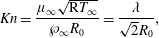 $$\begin{eqnarray}Kn=\frac{\unicode[STIX]{x1D707}_{\infty }\sqrt{\text{R}T_{\infty }}}{{\wp}_{\infty }R_{0}}=\frac{\unicode[STIX]{x1D706}}{\sqrt{2}R_{0}},\end{eqnarray}$$
where
 $\unicode[STIX]{x1D707}_{\infty }$
is the gas viscosity coefficient at the reference state. The mean free path,
 $\unicode[STIX]{x1D706}$
, is related to the usual definition of the mean free path
 $\ell _{0}$
(Sone Reference Sone2007) by
 $$\begin{eqnarray}\unicode[STIX]{x1D706}=\frac{\sqrt{\unicode[STIX]{x03C0}}}{2}A\ell _{0}.\end{eqnarray}$$
Here,
 $A=1.27$
for the hard-sphere model and
 $A=1$
for the BGK model, which gives the same fluid viscosity for different models and allows for a consistent comparison. For brevity, the hat will be removed hereafter, and unless otherwise stated, all variables will be given in dimensionless form.
For the linearised equations, only terms that are linear in deviations from the reference equilibrium state are considered. Accordingly, dimensionless and linearised conservation laws for mass, momentum and energy, in spherically symmetric coordinates, read
 $$\begin{eqnarray}\frac{1}{r^{2}}\frac{\unicode[STIX]{x2202}(r^{2}v)}{\unicode[STIX]{x2202}r}=0,\quad \frac{\unicode[STIX]{x2202}p}{\unicode[STIX]{x2202}r}+\frac{1}{r^{3}}\frac{\unicode[STIX]{x2202}(r^{3}\unicode[STIX]{x1D70E})}{\unicode[STIX]{x2202}r}=0,\quad \frac{1}{r^{2}}\frac{\unicode[STIX]{x2202}(r^{2}q)}{\unicode[STIX]{x2202}r}=0,\end{eqnarray}$$
which contain the normal component of the viscous stress,
 $\unicode[STIX]{x1D70E}$
and the radial heat flux,
 $q$
as unknowns. The various theories for transport provide equations for stress and heat flux which are presented in the following subsections.
3.1 Linearised NSF equations
In the dimensionless form and one-dimensional spherical geometry, the NSF constitutive laws for stress and heat flux are given by
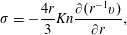 $$\begin{eqnarray}\displaystyle & \displaystyle \unicode[STIX]{x1D70E}=-\frac{4r}{3}Kn\frac{\unicode[STIX]{x2202}(r^{-1}v)}{\unicode[STIX]{x2202}r}, & \displaystyle\end{eqnarray}$$
 $$\begin{eqnarray}\displaystyle & \displaystyle q=-\frac{5Kn}{2Pr}\frac{\unicode[STIX]{x2202}\unicode[STIX]{x1D703}}{\unicode[STIX]{x2202}r}. & \displaystyle\end{eqnarray}$$
Here, the Prandtl number
 $Pr$
=
 $2/3$
for Maxwell molecules (MM) model and
 $Pr$
=
 $1$
for the BGK model.
The linearised form of the mass and momentum conservation laws (3.4) along with the constitutive relation for stress tensor (3.5) give the Stokes equations. In this case, the flow problem decouples from the Fourier-based energy problem, so that non-equilibrium cross-effects, such as thermal stress and non-Fourier heat flux (Sone Reference Sone2007; Rana et al. Reference Rana, Torrilhon and Struchtrup2013), cannot be predicted by the NSF system. High-order macroscopic models based on moment equations are developed to describe these effects.
3.2 Higher-order moment equations
The balance equations for the heat-flux vector and stress tensor follow from the Boltzmann equation as
 $$\begin{eqnarray}\displaystyle & \displaystyle \frac{8r}{15}\frac{\unicode[STIX]{x2202}(r^{-1}q)}{\unicode[STIX]{x2202}r}+\frac{1}{r^{4}}\frac{\unicode[STIX]{x2202}(r^{4}m)}{\unicode[STIX]{x2202}r}=-\frac{1}{Kn}\left[\unicode[STIX]{x1D70E}+\frac{4r}{3}Kn\frac{\unicode[STIX]{x2202}(r^{-1}v)}{\unicode[STIX]{x2202}r}\right], & \displaystyle\end{eqnarray}$$
 $$\begin{eqnarray}\displaystyle & \displaystyle \frac{1}{r^{3}}\frac{\unicode[STIX]{x2202}(r^{3}\unicode[STIX]{x1D70E})}{\unicode[STIX]{x2202}r}+\frac{1}{2r^{3}}\frac{\unicode[STIX]{x2202}(r^{3}R)}{\unicode[STIX]{x2202}r}+\frac{1}{6}\frac{\unicode[STIX]{x2202}\unicode[STIX]{x1D6E5}}{\unicode[STIX]{x2202}r}=-\frac{Pr}{Kn}\left[q+\frac{5}{2}\frac{Kn}{Pr}\frac{\unicode[STIX]{x2202}\unicode[STIX]{x1D703}}{\unicode[STIX]{x2202}r}\right]. & \displaystyle\end{eqnarray}$$
3.2.1 R13 constitutive relations
The balance equations (3.7) do not form a closed set, since they contain additional higher moments
 $m$
,
 $R$
and
 $\unicode[STIX]{x1D6E5}$
. In G13 theory,
 $m$
,
 $R$
and
 $\unicode[STIX]{x1D6E5}$
all are set to zero. A non-vanishing closure for these higher-order moments is given by the R13 constitutive relations (Struchtrup Reference Struchtrup2005). The linear R13 constitutive relations, for the considered geometry, take the following form
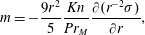 $$\begin{eqnarray}\displaystyle & \displaystyle m=-\frac{9r^{2}}{5}\frac{Kn}{Pr_{M}}\frac{\unicode[STIX]{x2202}(r^{-2}\unicode[STIX]{x1D70E})}{\unicode[STIX]{x2202}r}, & \displaystyle\end{eqnarray}$$
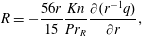 $$\begin{eqnarray}\displaystyle & \displaystyle R=-\frac{56r}{15}\frac{Kn}{Pr_{R}}\frac{\unicode[STIX]{x2202}(r^{-1}q)}{\unicode[STIX]{x2202}r}, & \displaystyle\end{eqnarray}$$
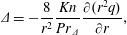 $$\begin{eqnarray}\displaystyle & \displaystyle \unicode[STIX]{x1D6E5}=-\frac{8}{r^{2}}\frac{Kn}{Pr_{\unicode[STIX]{x1D6E5}}}\frac{\unicode[STIX]{x2202}(r^{2}q)}{\unicode[STIX]{x2202}r}, & \displaystyle\end{eqnarray}$$
 $Pr_{M}$
,
 $Pr_{R}$
and
 $Pr_{\unicode[STIX]{x1D6E5}}$
depend upon the choice of inter-molecular potential function appearing in Boltzmann collision operator. For the MM model they are given by
 $Pr=2/3$
,
 $Pr_{M}=3/2$
,
 $Pr_{R}=7/6$
,
 $Pr_{\unicode[STIX]{x1D6E5}}=2/3$
and all are
 $1$
for BGK approximations (Truesdell & Muncaster Reference Truesdell and Muncaster1980; Gu & Emerson Reference Gu and Emerson2009).
The conservation laws (3.4), the balance equations for heat-flux vector and stress tensor (3.7) along with the constitutive relations (3.8) form the R13 equations.
3.2.2 R26 constitutive relations
The 26-moment theory consists of the conservation laws, the balance equations for the heat flux and stress and the balance equations for the higher moments,
 $\unicode[STIX]{x1D62E}_{ijk}$
,
 $\unicode[STIX]{x1D619}_{ij}$
and
 $\unicode[STIX]{x1D6E5}$
. The evolution equations for
 $\unicode[STIX]{x1D62E}_{ijk}$
,
 $\unicode[STIX]{x1D619}_{ij}$
and
 $\unicode[STIX]{x1D6E5}$
were obtained from the Boltzmann equation in Gu & Emerson (Reference Gu and Emerson2009), which for the present problem read
 $$\begin{eqnarray}\displaystyle & \displaystyle \frac{9r^{2}}{35}\frac{\unicode[STIX]{x2202}(r^{-2}R)}{\unicode[STIX]{x2202}r}+\frac{1}{r^{5}}\frac{\unicode[STIX]{x2202}(r^{5}\unicode[STIX]{x1D6F7})}{\unicode[STIX]{x2202}r}=-\frac{Pr_{M}}{Kn}\left[m+\frac{9r^{2}}{5}\frac{Kn}{Pr_{M}}\frac{\unicode[STIX]{x2202}(r^{-2}\unicode[STIX]{x1D70E})}{\unicode[STIX]{x2202}r}\right], & \displaystyle\end{eqnarray}$$
 $$\begin{eqnarray}\displaystyle & \displaystyle \frac{2}{r^{4}}\frac{\unicode[STIX]{x2202}(r^{4}m)}{\unicode[STIX]{x2202}r}+\frac{4r}{15}\frac{\unicode[STIX]{x2202}(r^{-1}\unicode[STIX]{x1D714})}{\unicode[STIX]{x2202}r}+\frac{1}{r^{4}}\frac{\unicode[STIX]{x2202}(r^{4}\unicode[STIX]{x1D713})}{\unicode[STIX]{x2202}r}=-\frac{Pr_{R}}{Kn}\left[R+\frac{56r}{15}\frac{Kn}{Pr_{R}}\frac{\unicode[STIX]{x2202}(r^{-1}q)}{\unicode[STIX]{x2202}r}\right], & \displaystyle\end{eqnarray}$$
 $$\begin{eqnarray}\displaystyle & \displaystyle \frac{1}{r^{2}}\frac{\unicode[STIX]{x2202}(r^{2}\unicode[STIX]{x1D714})}{\unicode[STIX]{x2202}r}=-\frac{Pr_{\unicode[STIX]{x1D6E5}}}{Kn}\left[\unicode[STIX]{x1D6E5}+\frac{8}{r^{2}}\frac{Kn}{Pr_{\unicode[STIX]{x1D6E5}}}\frac{\unicode[STIX]{x2202}(r^{2}q)}{\unicode[STIX]{x2202}r}\right]. & \displaystyle\end{eqnarray}$$
As for the NSF and the R13 cases, constitutive relations are needed to express the fluxes
 $\unicode[STIX]{x1D6F7}$
,
 $\unicode[STIX]{x1D713}$
and
 $\unicode[STIX]{x1D714}$
, to form a closed system. The R26 equations include the constitutive relations for these higher-order terms as (Gu & Emerson Reference Gu and Emerson2009)
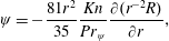
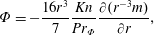 $$\begin{eqnarray}\displaystyle & \displaystyle \unicode[STIX]{x1D6F7}=-\frac{16r^{3}}{7}\frac{Kn}{Pr_{\unicode[STIX]{x1D6F7}}}\frac{\unicode[STIX]{x2202}(r^{-3}m)}{\unicode[STIX]{x2202}r}, & \displaystyle\end{eqnarray}$$
 $$\begin{eqnarray}\displaystyle & \displaystyle \unicode[STIX]{x1D713}=-\frac{81r^{2}}{35}\frac{Kn}{Pr_{\unicode[STIX]{x1D713}}}\frac{\unicode[STIX]{x2202}(r^{-2}R)}{\unicode[STIX]{x2202}r}, & \displaystyle\end{eqnarray}$$
 $$\begin{eqnarray}\displaystyle & \displaystyle \unicode[STIX]{x1D714}=-\frac{7Kn}{3}\frac{\unicode[STIX]{x2202}\unicode[STIX]{x1D6E5}}{\unicode[STIX]{x2202}r}-\frac{4}{r^{3}}Kn\frac{\unicode[STIX]{x2202}(r^{3}R)}{\unicode[STIX]{x2202}r}, & \displaystyle\end{eqnarray}$$
 $Pr_{\unicode[STIX]{x1D6F7}}$
 $=2.097$
and
 $Pr_{\unicode[STIX]{x1D713}}=1.698$
for MM and
 $Pr_{\unicode[STIX]{x1D6F7}}=Pr_{\unicode[STIX]{x1D713}}=1$
for the BGK model. The constitutive relations (3.10) with balance equations (3.9) and (3.7) and conservation laws (3.4) form the system of the R26 equations.
Comparison of the R13 constitutive relations (3.8) with the balance equations (3.9) reveals that the R13 constitutive relations (3.8) stem from a Chapman–Enskog expansion of (3.9) in
 $Kn$
, i.e. taking the right-hand side of (3.9) to be zero. Likewise, the R26 constitutive relations (3.10) follow from the Chapman–Enskog expansion of the evolution equations for the moments
 $\unicode[STIX]{x1D719}_{ijkl}$
,
 $\unicode[STIX]{x1D713}_{ijk}$
and
 $\unicode[STIX]{x1D714}_{i}$
from the 45-moment theory.
In the next section, we shall derive analytic solutions to the NSF, R13 and R26 equations for the spherical geometry and then in § 5 formulate and apply the boundary conditions required for the evaporation problem.
4 Analytical solutions of the moment equations
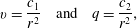
Due to the linearity of the equations and the simple geometry, we have found that all equations can be solved analytically. By integrating the mass and energy conservation laws (3.4a,c ), we immediately find
 $$\begin{eqnarray}v=\frac{c_{1}}{r^{2}}\quad \text{and}\quad q=\frac{c_{2}}{r^{2}},\end{eqnarray}$$
where
 $c_{1}$
and
 $c_{2}$
are integration coefficients. These solutions are obtained from the conservation laws without any assumption on constitutive relations and therefore they are valid for all values of the Knudsen number. The integration coefficients
 $c_{1}$
and
 $c_{2}$
, however, depend on other field variables through boundary conditions, and consequently, these depend on the constitutive relations.
4.1 Solution to the NSF equations
Substitution of the velocity and heat flux from (4.1) into the NSF constitutive equations (3.1), leads to the solutions
 $$\begin{eqnarray}\unicode[STIX]{x1D70E}=\frac{4Knc_{1}}{r^{3}}\quad \text{and}\quad \unicode[STIX]{x1D703}=c_{3}+\frac{2Pr}{5Kn}\frac{c_{2}}{r},\end{eqnarray}$$
and the momentum equation (3.4b ) gives
 $$\begin{eqnarray}p=c_{4}.\end{eqnarray}$$
Applying the far-field boundary conditions, we find that
 $c_{3}=c_{4}=0$
, since
 $$\begin{eqnarray}\lim _{r\rightarrow \infty }\unicode[STIX]{x1D703}=0\quad \text{and}\quad \lim _{r\rightarrow \infty }p=0.\end{eqnarray}$$
Therefore, for the given flow configurations, the solutions of the NSF equations include two integration constants,
 $c_{1}$
and
 $c_{2}$
. These constants need to be fixed from two boundary conditions at the interface at
 $r=1$
.
4.2 Solution to the R13 equations
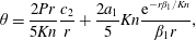
The integration of the heat-flux and stress balance equations (3.7) and use of the R13 constitutive relations (3.8) with the solutions (4.1), give
 $$\begin{eqnarray}\displaystyle & \displaystyle \unicode[STIX]{x1D70E}=\frac{4Knc_{1}}{r^{3}}+\frac{8Knc_{2}}{5r^{3}}-3a_{1}\left(Kn^{3}+Kn^{2}r\unicode[STIX]{x1D6FD}_{1}+Kn\frac{r^{2}\unicode[STIX]{x1D6FD}_{1}^{2}}{3}\right)\frac{\text{e}^{-r\unicode[STIX]{x1D6FD}_{1}/Kn}}{\unicode[STIX]{x1D6FD}_{1}^{3}r^{3}}, & \displaystyle\end{eqnarray}$$
 $$\begin{eqnarray}\displaystyle & \displaystyle \unicode[STIX]{x1D703}=\frac{2Pr}{5Kn}\frac{c_{2}}{r}+\frac{2a_{1}}{5}Kn\frac{\text{e}^{-r\unicode[STIX]{x1D6FD}_{1}/Kn}}{\unicode[STIX]{x1D6FD}_{1}r}, & \displaystyle\end{eqnarray}$$
 $\unicode[STIX]{x1D6FD}_{1}=\sqrt{5Pr_{M}}/3$
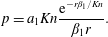
. In (4.5) we have already used the far-field conditions (4.4). Similarly, the momentum equations (3.4b
) and (4.5a
) give the pressure
 $$\begin{eqnarray}p=a_{1}Kn\frac{\text{e}^{-r\unicode[STIX]{x1D6FD}_{1}/Kn}}{\unicode[STIX]{x1D6FD}_{1}r}.\end{eqnarray}$$
The R13 equations therefore allow for a non-uniform pressure in the gas that decays exponentially with the scaled distance
 $r\unicode[STIX]{x1D6FD}_{1}$
from the interface. It is a purely non-equilibrium effect caused by the Knudsen layer. The non-uniform pressure has been observed in molecular dynamics (MD) simulations (Holyst & Litniewski Reference Hołyst and Litniewski2008; Cheng et al.
Reference Cheng, Lechman, Plimpton and Grest2011; Rana et al.
Reference Rana, Ravichandran, Park and Myong2016), kinetic theory computations (Sone & Onishi Reference Sone and Onishi1978) and previous works (Taheri et al.
Reference Taheri, Rana, Torrilhon and Struchtrup2009; Taheri & Struchtrup Reference Taheri and Struchtrup2009; Struchtrup & Taheri Reference Struchtrup and Taheri2011) for different flow configurations. Evidently, the NSF equations fail to capture this phenomenon.
Solutions (4.5)–(4.6) of the R13 equations have three integration constants,
 $c_{1,2}$
and
 $a_{1}$
, which need to be determined from the three boundary conditions at
 $r=1$
.
4.3 Solution to the R26 equations
The integration of the R26 equations is more involved and can be found in the appendix; here we present only the final results. The pressure and normal stress are given as the superposition of three decaying exponentials expressed as
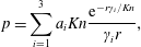 $$\begin{eqnarray}\displaystyle & \displaystyle p=\mathop{\sum }_{i=1}^{3}a_{i}Kn\frac{\text{e}^{-r\unicode[STIX]{x1D6FE}_{i}/Kn}}{\unicode[STIX]{x1D6FE}_{i}r}, & \displaystyle\end{eqnarray}$$
 $$\begin{eqnarray}\displaystyle & \displaystyle \unicode[STIX]{x1D70E}=\frac{4Kn~c_{1}}{r^{3}}+\frac{8Kn~c_{2}}{5r^{3}}-3\mathop{\sum }_{i=1}^{3}a_{i}\left(Kn^{3}+Kn^{2}r\unicode[STIX]{x1D6FE}_{i}+Kn\frac{r^{2}\unicode[STIX]{x1D6FE}_{i}^{2}}{3}\right)\frac{\text{e}^{-r\unicode[STIX]{x1D6FE}_{i}/Kn}}{r^{3}\unicode[STIX]{x1D6FE}_{i}^{3}}, & \displaystyle\end{eqnarray}$$
 $\unicode[STIX]{x1D6FE}_{i}\in \mathbb{R}^{+}$
for the MM model and BGK model are given in table 1.
Interestingly, the normal stress
 $\unicode[STIX]{x1D70E}$
(4.7b
) has three contributions: (i) Newtonian stress (with
 $Kn\,c_{1}$
), (ii) thermal stress (with
 $Kn\,c_{2}$
) and (iii) Knudsen layer contributed stress (with exponentials). The origin of these different contributions to the stress are best explained by the stress balance equation (3.7a
) from which the Newtonian stress and thermal stress arise due to the velocity gradient and the heat-flux gradient terms, respectively, and derivative of the higher-order moment
 $m$
produces the Knudsen layer. The only non-zero contribution to the pressure (4.7a
) is due to Knudsen layer, given by the radial momentum conservation (3.4b
).
As the NSF equations are only accurate up to first order in
 $Kn$
(by Chapman–Enskog expansion), they capture the Newtonian stress (first order) but not the thermal stress (second order). The effect of these different contributions on the vapour flow will be studied later in § 9.
The temperature from the R26 equations reads
 $$\begin{eqnarray}\unicode[STIX]{x1D703}=\frac{2Pr}{5Kn}\frac{c_{2}}{r}+\mathop{\sum }_{i=1}^{3}a_{i}Kn(k_{1}\unicode[STIX]{x1D6FE}_{i}^{4}+k_{2}\unicode[STIX]{x1D6FE}_{i}^{2}+k_{3})\frac{\text{e}^{-r\unicode[STIX]{x1D6FE}_{i}/Kn}}{r\unicode[STIX]{x1D6FE}_{i}^{3}}.\end{eqnarray}$$
The temperature
 $\unicode[STIX]{x1D703}$
has a Fourier contribution,
 $(2Pr/5Kn)(c_{2}/r)$
, which comes from the right-hand side terms in the heat-flux balance equation (3.7b
), plus an additional contribution due to the Knudsen layer (superposition of exponential functions), which describes the influence of higher moments in (3.7b
). The coefficient
 $k_{1}$
,
 $k_{2}$
and
 $k_{3}$
in (4.8) depend on the collision model, they are given in equation (A 6) of the appendix.
The Knudsen layer coefficients
 $\unicode[STIX]{x1D6FE}_{i}$
associated with the R26 equations for BGK and Maxwell molecules (MM) models.

The solutions of the R26 equations for
 $p$
,
 $\unicode[STIX]{x1D70E}$
and
 $\unicode[STIX]{x1D703}$
given in (4.7) and (4.8) and other variables (given in appendix A) contain
 $5$
integration constants,
 $c_{1,2}$
and
 $a_{1,2,3}$
. These constants are to be evaluated from interface conditions at
 $r=1$
. The boundary conditions for NSF, R13 and R26 equations are derived in the next section.
5 Formulation of the boundary conditions
The boundary conditions for evaporating and condensing interfaces for the R13 equations have been derived by Struchtrup & Frezzotti (Reference Struchtrup and Frezzotti2016), and here we follow the same steps for the derivation of the evaporating/condensing interface conditions for the R26 equations.
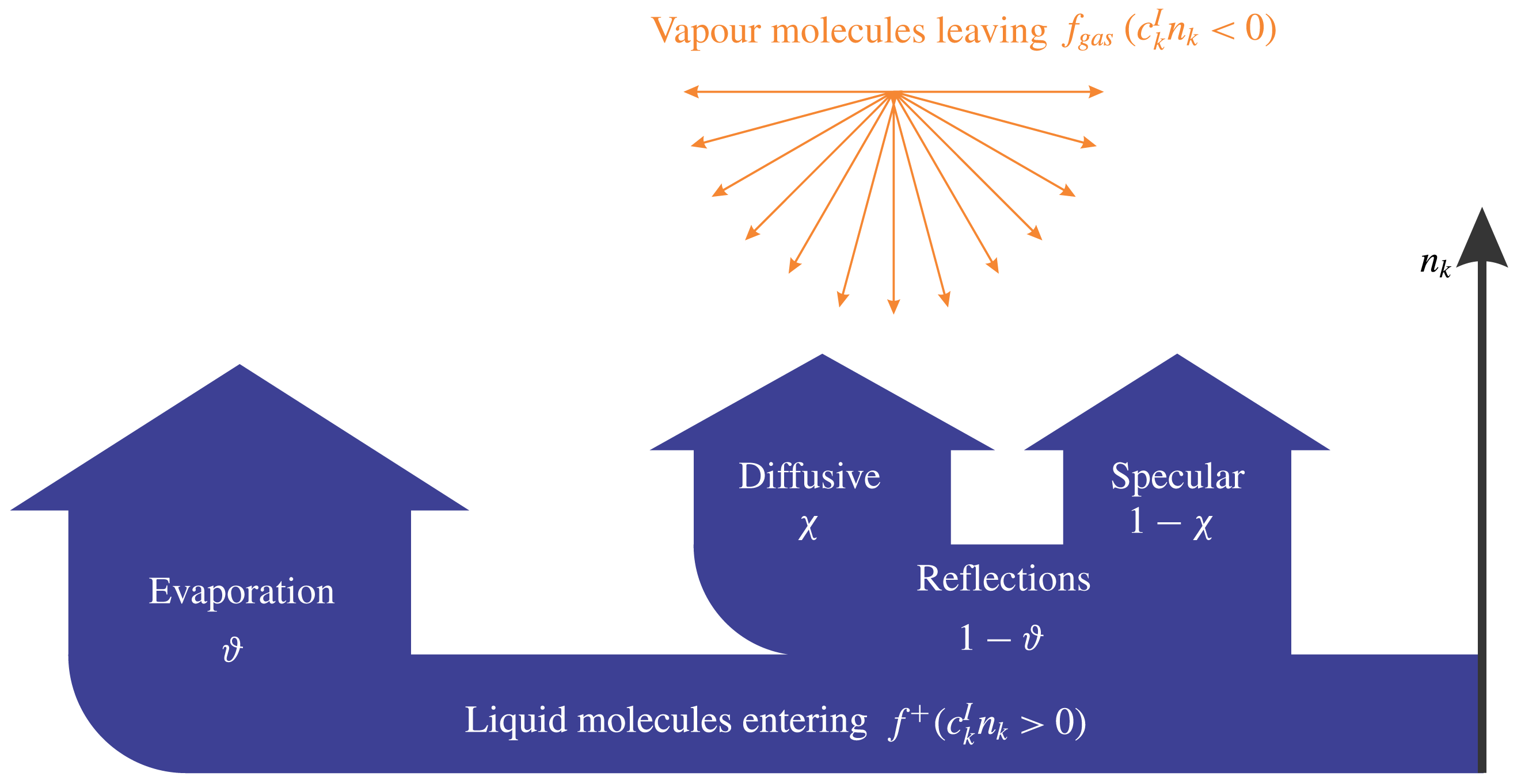
A phase interface, where particles approaching the interface from the vapour phase (
 $c_{k}^{I}n_{k}<0$
) are described by the Grad 45-moment (G45) distribution function
 $f|_{G45}$
and molecules entering the gas (
 $c_{k}^{I}n_{k}\geqslant 0$
) are distributed according to a known distribution
 $f^{+}$
, see figure 2. Note that
 $f|_{G45}$
reconstructs the distribution function in Hermite polynomials such that it reproduces all 45 moments appearing in the R26 equations. Similarly, for the NSF and R13 equations, G13 and G26 distribution functions are used, respectively.
Schematic of the evaporation and reflection (specular and diffusive) process at the liquid–vapour interface. The distribution of molecules entering from vapour phase is approximated by Grad’s distribution function, i.e.
 $f_{gas}\simeq f|_{G45}$
in equation (5.1).
Here,
 $n_{k}$
denotes the normal vector to the wall pointing into the vapour phase, and
 $c_{k}^{I}$
is the velocity of vapour molecules in the reference frame of the interface. The explicit form of
 $f|_{G45}$
can be found in the literature, for example by Gu & Emerson (Reference Gu and Emerson2009). The distribution of molecules entering the gas is written as (Struchtrup & Frezzotti Reference Struchtrup and Frezzotti2016)
 $$\begin{eqnarray}f^{+}=\unicode[STIX]{x1D717}f_{M}(\unicode[STIX]{x1D703}_{l},p_{l};c_{k}^{I})+(1-\unicode[STIX]{x1D717})\left[\unicode[STIX]{x1D712}f_{M}(T,p;c_{k}^{I})+(1-\unicode[STIX]{x1D712})f|_{G45}(T,p;c_{k}^{\ast })\right],\end{eqnarray}$$
where,
 $\unicode[STIX]{x1D717}$
is defined as the evaporation/condensation coefficient, and
 $\unicode[STIX]{x1D712}$
is the accommodation coefficient, defined as the fraction of reflected molecules being thermalised. Here
 $c_{k}^{\ast }$
represents the specularly reflected values of
 $c_{k}^{I}$
with respect to
 $n_{k}$
. In (5.1),
 $\unicode[STIX]{x1D703}_{l}$
is the temperature of the liquid phase at the interface and
 $p_{l}$
is saturation pressure at
 $\unicode[STIX]{x1D703}_{l}$
, following the definitions and the notations in (3.1). Note that, for non-evaporating interfaces (
 $\unicode[STIX]{x1D717}=0$
), the above model reduces to the Maxwell accommodation model (Torrilhon & Struchtrup Reference Torrilhon and Struchtrup2008; Gu & Emerson Reference Gu and Emerson2009).
At the interface, the distribution function
 $\bar{f}$
of the vapour molecules is therefore written as
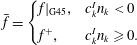 $$\begin{eqnarray}\bar{f}=\left\{\begin{array}{@{}ll@{}}f|_{\text{G45}}, & c_{k}^{I}n_{k}<0\\ f^{+}, & c_{k}^{I}n_{k}\geqslant 0.\end{array}\right.\end{eqnarray}$$
Once the distribution function at the interface is defined, the process of deriving the interface boundary conditions is the same as that for the wall boundary conditions (Torrilhon & Struchtrup Reference Torrilhon and Struchtrup2008; Gu & Emerson Reference Gu and Emerson2009). Again, assuming small deviations, i.e.
 $|p_{l}|\ll 1$
and
 $|\unicode[STIX]{x1D703}_{l}|\ll 1$
, linearisation of the distribution (5.2) can be performed. The distribution function (5.2) is further simplified when relations (2.8) and (2.9) specifying the flow configuration are introduced.
5.1 Boundary conditions for NSF, R13 and R26
The evaporation and condensation boundary conditions for the R26 equations read
 $$\begin{eqnarray}\displaystyle & \displaystyle v=-\unicode[STIX]{x1D70D}\left(p-p_{l}-\frac{{\mathcal{T}}}{2}+\frac{\unicode[STIX]{x1D70E}}{2}-\frac{R}{28}-\frac{\unicode[STIX]{x1D6F7}}{24}\right), & \displaystyle\end{eqnarray}$$
 $$\begin{eqnarray}\displaystyle & \displaystyle q+\frac{v}{2}=-\unicode[STIX]{x1D70F}\left(2{\mathcal{T}}+\frac{\unicode[STIX]{x1D70E}}{2}+\frac{5R}{28}+\frac{\unicode[STIX]{x1D6E5}}{15}-\frac{\unicode[STIX]{x1D6F7}}{12}\right), & \displaystyle\end{eqnarray}$$
 $$\begin{eqnarray}\displaystyle & \displaystyle m+\frac{2\,v}{5}=\unicode[STIX]{x1D70F}\left(\frac{2{\mathcal{T}}}{5}-\frac{7\unicode[STIX]{x1D70E}}{5}-\frac{R}{14}+\frac{\unicode[STIX]{x1D6E5}}{75}-\frac{13\unicode[STIX]{x1D6F7}}{30}\right), & \displaystyle\end{eqnarray}$$
 $$\begin{eqnarray}\displaystyle & \displaystyle \unicode[STIX]{x1D713}-\frac{6\,v}{5}=\unicode[STIX]{x1D70F}\left(\frac{6{\mathcal{T}}}{5}+\frac{9\unicode[STIX]{x1D70E}}{5}-\frac{93R}{70}+\frac{\unicode[STIX]{x1D6E5}}{5}-\frac{\unicode[STIX]{x1D6F7}}{2}\right), & \displaystyle\end{eqnarray}$$
 $$\begin{eqnarray}\displaystyle & \displaystyle \unicode[STIX]{x1D714}-3v=\unicode[STIX]{x1D70F}\left(8{\mathcal{T}}+2\unicode[STIX]{x1D70E}-R-\frac{4\unicode[STIX]{x1D6E5}}{3}\right). & \displaystyle\end{eqnarray}$$
 $$\begin{eqnarray}\unicode[STIX]{x1D70D}=\frac{\unicode[STIX]{x1D717}}{2-\unicode[STIX]{x1D717}}\sqrt{\frac{2}{\unicode[STIX]{x03C0}}}\quad \text{ and }\quad \unicode[STIX]{x1D70F}=\frac{\unicode[STIX]{x1D717}+\unicode[STIX]{x1D712}(1-\unicode[STIX]{x1D717})}{2-\unicode[STIX]{x1D717}-\unicode[STIX]{x1D712}(1-\unicode[STIX]{x1D717})}\sqrt{\frac{2}{\unicode[STIX]{x03C0}}},\end{eqnarray}$$
and
 ${\mathcal{T}}=\unicode[STIX]{x1D703}-\unicode[STIX]{x1D703}_{l}$
denotes the temperature jump at the interface. As expected, for non-evaporating interfaces (
 $\unicode[STIX]{x1D717}=0$
), the above interface boundary conditions are reduced to the wall boundary conditions for the R26 equations derived by Gu & Emerson (Reference Gu and Emerson2009).
The R13 equations are obtained from the first three equations (5.3a–c
), with
 $R$
,
 $m$
and
 $\unicode[STIX]{x1D6E5}$
replaced by the R13 constitutive laws (3.8) and
 $\unicode[STIX]{x1D6F7}=0$
.
The NSF boundary conditions, permitting a temperature jump, require that both the stress and the heat flux in (5.3a
) and (5.3b
) are replaced by the NSF laws (3.1) alongside
 $R=m=\unicode[STIX]{x1D6E5}=\unicode[STIX]{x1D6F7}=0$
.
5.2 Comparison with classical theories
At thermodynamic equilibrium, the chemical potential and temperature are assumed continuous across the liquid/vapour interface. These conditions lead to the Clausius–Clapeyron relations, i.e. a relation between the saturation pressure and temperature at equilibrium. However, when the interface is not under local equilibrium conditions, it is usually assumed that the mass flux
 $j$
(in dimensional form) obeys the Hertz–Knudsen–Schrage (HKS) relation, derived from the kinetic theory of gases as (Schrage Reference Schrage1953)
 $$\begin{eqnarray}j=\frac{1}{2-\unicode[STIX]{x1D70E}_{c}}\sqrt{\frac{2}{\unicode[STIX]{x03C0}}}\left(\unicode[STIX]{x1D70E}_{e}\frac{{\wp}_{l}}{\sqrt{\text{R}T_{l}}}-\unicode[STIX]{x1D70E}_{c}\frac{{\wp}}{\sqrt{\text{R}T}}\right)\!,\end{eqnarray}$$
where
 $\unicode[STIX]{x1D70E}_{e}$
and
 $\unicode[STIX]{x1D70E}_{c}$
denote the evaporation and condensation coefficients, respectively, representing the fraction of molecules that strike the interface and change phases from their initial liquid or vapour states, respectively. When written in the dimensionless and linearised form, the HKS relation (5.5) for
 $\unicode[STIX]{x1D70E}_{c}=\unicode[STIX]{x1D70E}_{e}=\unicode[STIX]{x1D717}$
reduces to
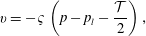 $$\begin{eqnarray}v=-\unicode[STIX]{x1D70D}\left(p-p_{l}-\frac{{\mathcal{T}}}{2}\right),\end{eqnarray}$$
which is the linear Hertz–Knudsen–Schrage (LHKS) relation.
In the standard approach, the HKS is combined with the equality of liquid and vapour temperatures at the interface, i.e.
 $$\begin{eqnarray}\unicode[STIX]{x1D703}=\unicode[STIX]{x1D703}_{l}.\end{eqnarray}$$
Comparing with our boundary conditions for the R26 equations, we see that (5.3a
) is a generalisation of the LHKS relation which contains the higher-order moments (
 $R,$
 $\unicode[STIX]{x1D6F7}$
) and an additional term (
 $\unicode[STIX]{x1D70E}/2$
) in (5.3a
) due to the geometric curvature. In what follows, the results obtained from macroscopic models are compared with the linearised Boltzmann solutions in order to determine the gains in accuracy from using the R13 or R26 theories over the classical one.
5.3 Summary of models
Below, we summarise the hierarchy of models which are to be investigated in the forthcoming sections. Each is composed of bulk equations for
 $r>1$
supplemented with boundary conditions at the droplet surface (
 $r=1$
).
-
(i) NSF: The NSF equations are used alongside LHKS given in (5.6) and the classical no-temperature-jump condition from (5.7). That is, the integration constants (
$c_{1,2}$
) appearing in the NSF solutions (4.1)–(4.3) are determined from the boundary conditions (5.6) and (5.7). -
(ii) NSF (+jump): The NSF equations are used with the mass-flux boundary condition (5.3a ) and the temperature jump boundary condition (5.3b ). These two boundary conditions give two integration constants (
$c_{1,2}$
) appearing in the NSF solutions (4.1)–(4.3). -
(iii) R13: The R13 moment equations are solved, with integration constants
$c_{1,2}$
and
$a_{1}$
in their solutions (4.1), (4.5) and (4.6) calculated from the first three boundary conditions (5.3a–c
). -
(iv) R26: The R26 moment equations are solved, with integration constants
$c_{1,2}$
and
$a_{1,2,3}$
appearing in the R26 solutions (4.1), (4.7) and (4.8) obtained from all five boundary conditions (5.3a–e
).


A Mathematica script can be found in the online supplementary material (available at https://doi.org/10.1017/jfm.2018.85), which computes and lists these integration constants for the NSF, R13 as well as the R26 equations.
6 Evaporation of a spherical drop as
$Kn\rightarrow 0$

As a starting point we consider
 $Kn\rightarrow 0$
for the two cases of pressure-driven flow (
 $p_{l}=1$
,
 $\unicode[STIX]{x1D703}_{l}=0$
) and temperature-driven flow (
 $p_{l}=0$
,
 $\unicode[STIX]{x1D703}_{l}=1$
), which allows us to compare the results with previously obtained solutions of the linearised Boltzmann equation (LBE).
To establish the limits of applicability of our analytic solutions, we will compare them with numerical solution of the LBE based on both the S-model (Chernyak & Margilevskiy Reference Chernyak and Margilevskiy1989), and hard-sphere molecules (Sone & Onishi Reference Sone and Onishi1978; Takata et al.
Reference Takata, Sone, Lhuilliere and Wakabayashi1998; Sone Reference Sone2007), for the case of complete evaporation (
 $\unicode[STIX]{x1D717}=1$
). Therefore, henceforth,
 $\unicode[STIX]{x1D717}=1$
.
6.1 Pressure-driven flow
$(p_{l}=1,\unicode[STIX]{x1D703}_{l}=0)$

The LBE with S-model predicts that the mass-flux coefficient
 $c_{1}\,(=vr^{2})\rightarrow 0.6654$
as
 $Kn\rightarrow 0$
(Chernyak & Margilevskiy Reference Chernyak and Margilevskiy1989) whilst Sone & Onishi (Reference Sone and Onishi1978) applied the asymptotic method to the LBE for hard-sphere molecules to obtain
 $c_{1}\rightarrow 0.6633$
as
 $Kn\rightarrow 0$
. The value 0.66–0.67 can be directly compared to those obtained from the macroscopic models, as tabulated in table 2, for a gas composed of Maxwell molecules and for the BGK model.
For both the R13 and R26 theories,
 $c_{1}$
is predicted to within two significant figures of the LBE result with very little dependence on the collision model used. In contrast, the NSF (+jump) model only agrees to one significant figure and the NSF fails to even match this. Interestingly, even in the limit
 $Kn\rightarrow 0$
where, naively, one may expect all of the models to coincide, including higher moments enables more accurate prediction of pressure-driven evaporative flow. This poor behaviour of macroscopic boundary conditions for the NSF equations stems from the approximation
 $f_{gas}\simeq f|_{G13}$
for molecules impinging the liquid from within the Knudsen layer.
Notably, many studies use fitting parameters, such as effective condensation coefficients or effective temperature jump coefficients, which are fitted to the asymptotic solutions to the kinetic equation for a specific problem. However, the boundary conditions used in this study contain no fitting parameters; hence the results presented are fully predictive and the model is not problem specific.
Results of pressure-driven calculations (
 $p_{l}=1$
,
 $\unicode[STIX]{x1D703}_{l}=0$
). Asymptotic values as
 $Kn\rightarrow 0$
of
 $c_{1}$
for different macroscopic models with complete evaporation (
 $\unicode[STIX]{x1D717}=1$
) for BGK and Maxwell molecules models. Note the LBE benchmark for
 $c_{1}$
is in the range 0.66–0.67.

For the pressure-driven case, the heat-flux coefficient
 $c_{2}\,(=qr^{2})\rightarrow 0$
as
 $Kn\rightarrow 0$
, for all the cases, including the LBE solutions from Chernyak & Margilevskiy (Reference Chernyak and Margilevskiy1989). Therefore, we study the
 $O(Kn)$
term as
 $Kn\rightarrow 0$
, i.e. we look at
 $\lim _{Kn\rightarrow 0}(c_{2}Pr/Kn)$
, which was calculated to be
 $-0.5250$
for the S-model (Chernyak & Margilevskiy Reference Chernyak and Margilevskiy1989).
As one can see from table 3, the NSF fails to predict a gradient in
 $c_{2}$
as
 $Kn\rightarrow 0$
whilst all the NSF(+jump)/R13/R26 theories provide reasonable agreement with the LBE results. Notably, the R26 theory gives the best prediction out of these models.
Results of pressure-driven calculations (
 $p_{l}=1$
,
 $\unicode[STIX]{x1D703}_{l}=0$
). Values of
 $\lim _{Kn\rightarrow 0}(c_{2}Pr/Kn)$
for different macroscopic models with complete evaporation (
 $\unicode[STIX]{x1D717}=1$
) for BGK and MM models. These should be compared to
 $-0.5250$
for the S-model (Chernyak & Margilevskiy Reference Chernyak and Margilevskiy1989).

6.2 Temperature-driven flow
$(p_{l}=0,\unicode[STIX]{x1D703}_{l}=1)$

Our benchmark results from the LBE equation (Chernyak & Margilevskiy Reference Chernyak and Margilevskiy1989) as
 $Kn\rightarrow 0$
are
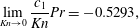 $$\begin{eqnarray}\displaystyle & \displaystyle \lim _{Kn\rightarrow 0}\frac{c_{1}}{Kn}Pr=-0.5293, & \displaystyle\end{eqnarray}$$
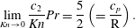 $$\begin{eqnarray}\displaystyle & \displaystyle \lim _{Kn\rightarrow 0}\frac{c_{2}}{Kn}Pr=\frac{5}{2}\left(=\frac{c_{p}}{\text{R}}\right). & \displaystyle\end{eqnarray}$$
The value for
 $\lim _{Kn\rightarrow 0}(c_{1}Pr/Kn)$
predicted by the moment equations for the temperature-driven case is the same as
 $\lim _{Kn\rightarrow 0}(c_{2}Pr/Kn)$
for the pressure-driven case. These values were discussed in § 6.1 and are tabulated in table 3. The equality of
 $c_{1}$
for temperature-driven case and
 $c_{2}$
for pressure-driven case follows from Onsager’s reciprocal relations (De Groot & Mazur Reference de Groot and Mazur1984; Takata et al.
Reference Takata, Sone, Lhuilliere and Wakabayashi1998).
All macroscopic models describe the correct asymptotic limit for
 $\lim _{Kn\rightarrow 0}(c_{2}Pr/Kn)=(5/2)$
, which follows from Fourier’s law (3.6).
In summary, our results indicate that the R26 equations with evaporation boundary conditions yield an excellent quantitative description in all cases, for both MM and BGK collision models, which are not matched by the NSF or R13 theories.
7 Evaporation from a planar surface: Knudsen layer structure and Ytrehus’ problem
Whilst no flow profiles within the Knudsen layer are available from kinetic theory for the case of an evaporating sphere, Sone and coauthors have examined the structure of Knudsen layers for evaporation/condensation from a planar interface (Sone & Onishi Reference Sone and Onishi1978; Takata et al. Reference Takata, Sone, Lhuilliere and Wakabayashi1998). The planar interface can be derived as a particular case of the solutions in the spherical geometry obtained in § 4, recovered by defining
 $$\begin{eqnarray}\unicode[STIX]{x1D702}=\frac{r-1}{Kn\sqrt{2}},\end{eqnarray}$$
and taking an asymptotic limit
 $Kn\rightarrow 0$
. Here,
 $\unicode[STIX]{x1D702}$
is the dimensionless distance from the interface, which is made dimensionless with the mean free path,
 $~\unicode[STIX]{x1D706}=\unicode[STIX]{x1D707}_{\infty }\sqrt{2\text{R}T_{\infty }}/p_{\infty }$
. It is convenient to introduce a dimensionless temperature defect
 $\unicode[STIX]{x1D6E9}$
as
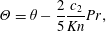 $$\begin{eqnarray}\unicode[STIX]{x1D6E9}=\unicode[STIX]{x1D703}-\frac{2}{5}\frac{c_{2}}{Kn}Pr,\end{eqnarray}$$
which has been defined so as to vanish for the NSF and NSF(+jump) models so that
 $\unicode[STIX]{x1D6E9}$
is a purely non-Fourier contribution to the temperature that only appears inside Knudsen layer.
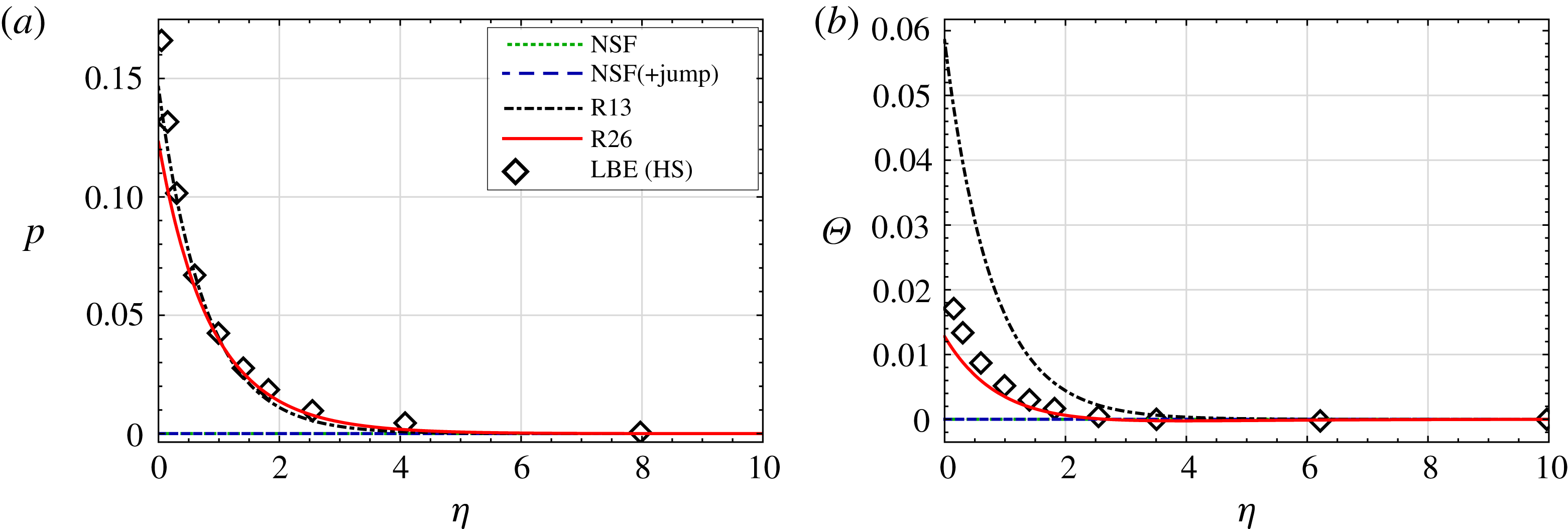
Knudsen layer functions in pressure-driven flow (
 $p_{l}=1$
,
 $\unicode[STIX]{x1D703}_{l}=0$
): curves of the normalised pressure
 $p$
(a) and the temperature defect
 $\unicode[STIX]{x1D6E9}$
(b) are plotted against scaled distance from the interface
 $\unicode[STIX]{x1D702}$
, for the NSF, R13 and R26 theories with complete evaporation (
 $\unicode[STIX]{x1D717}=1$
). Note that NSF curves do not deviate from zero. Also plotted are the results for the LBE from Sone & Onishi (Reference Sone and Onishi1978).
7.1 Knudsen layer: pressure-driven flow
$(p_{l}=1,\unicode[STIX]{x1D703}_{l}=0)$

Figure 3 compares the pressure
 $p$
and temperature defect
 $\unicode[STIX]{x1D6E9}$
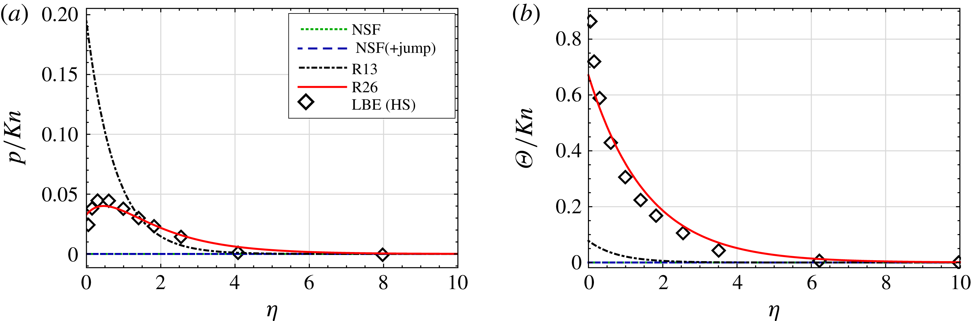
for the different macroscopic theories with the results by Sone & Onishi (Reference Sone and Onishi1978). The results indicate that NSF and NSF(+jump) cannot describe non-zero pressure and temperature defects, whilst the Knudsen layer profile for pressure (figure 3
a) is captured quite accurately by both the R13 and R26 equations. However, the temperature defect
 $\unicode[STIX]{x1D6E9}$
near the wall (figure 3
b) is only accurately predicted by the R26 equations, with the LBE result around three times smaller than that predicted by the R13 equations at
 $\unicode[STIX]{x1D702}=0$
.
Knudsen layer functions in temperature-driven flow (
 $p_{l}=0$
,
 $\unicode[STIX]{x1D703}_{l}=1$
): curves of the normalised pressure
 $p/Kn$
(a) and the temperature defect
 $\unicode[STIX]{x1D6E9}/Kn$
(b) are plotted against scaled distance from the interface
 $\unicode[STIX]{x1D702}$
, for the NSF, R13 and R26 theories with complete evaporation (
 $\unicode[STIX]{x1D717}=1$
). Also plotted are the results for the LBE from Sone & Onishi (Reference Sone and Onishi1978).
7.2 Knudsen layer: temperature-driven flow
$(p_{l}=0,\unicode[STIX]{x1D703}_{l}=1)$

Unlike the pressure-driven case, in temperature-driven flow (figure 4
a,b), the pressure and temperature defect both vanish as
 $Kn\rightarrow 0$
with
 $O(Kn)$
. Therefore, to obtain the next-order terms in
 $Kn$
, the results are divided with the Knudsen number before the limit is taken to recover the most relevant values in this limit.
Figure 4(a) shows that the LBE benchmark for the pressure profile exhibits a maxima at a finite distance from the boundary, inside the Knudsen layer, which is only captured by the R26 model. According to our analytical solutions, the ultimate source of the fascinating behaviour can be traced to the combination of unique exponentials appearing in the solution of the R26 equations in (4.7a
). The actual Knudsen layer is a linear superposition of many exponential functions
 $\text{e}^{-r\unicode[STIX]{x1D6FE}_{i}/Kn}$
(Struchtrup Reference Struchtrup2008) – with different coefficients
 $\unicode[STIX]{x1D6FE}_{i}$
– the R13 equations give only one such contribution so that non-monotonic behaviour cannot be captured. In contrast, the R26 system provides three exponential functions to form the Knudsen layer, thus capturing the more complex behaviour. For the temperature defect (figure 4
b) the R26 solution still provides far greater accuracy in the Knudsen layer.
7.3 Summary of the behaviour of the Knudsen layer
The Knudsen layer is the kinetic boundary layer, found in the region of gas flow adjacent to the boundary. Whilst the R13 and R26 theories pick up the existence of Knudsen layer, it is the R26 theory which has access to three exponential functions to approximate this region. Therefore, R26 can (i) capture intricate qualitative features of the LBE solution and (ii) provide a good quantitative accuracy. Consequently, from here on, we focus on comparing the R26 equations with the classical approach of the NSF and its extension NSF(+jump). Henceforth, we consider only MM collision model.
7.4 Comparison of predicted mass- and heat-flux coefficients for evaporation from a planar surface (Ytrehus’ problem)
As a special case, we can find relevant flow coefficients for the steady evaporation from a planar surface into a half-space by using the reduced distance (7.1) and taking an asymptotic limit
 $Kn\rightarrow 0$
. The half-space evaporation problem, often referred to as Ytrehus’ problem (Ytrehus & Ostmo Reference Ytrehus and Ostmo1996), concerns an evaporating liquid surface kept at a temperature
 $\unicode[STIX]{x1D703}_{l}$
and evaporation pressure
 $p_{l}$
. Far from the interface, the flow is in a uniform equilibrium state with bulk velocity
 $v=v_{\infty }>0$
and
 $q=0$
. With the
 $v_{\infty }$
and
 $q$
prescribed, the coefficients
 $c_{1}$
and
 $c_{2}$
in (4.1) are
 $$\begin{eqnarray}c_{1}=v_{\infty }\quad \text{and }\quad c_{2}=0,\end{eqnarray}$$
and the temperature
 $\unicode[STIX]{x1D703}_{l}$
and evaporation pressure
 $p_{l}$
are determined from the boundary conditions. Defining
 $$\begin{eqnarray}p_{l}=\unicode[STIX]{x1D6FC}_{p}\frac{v_{\infty }}{\sqrt{2}}\quad \text{ and }\quad \unicode[STIX]{x1D703}_{l}=\unicode[STIX]{x1D6FC}_{\unicode[STIX]{x1D703}}\frac{v_{\infty }}{\sqrt{2}},\end{eqnarray}$$
where the coefficients
 $\unicode[STIX]{x1D6FC}_{p}$
and
 $\unicode[STIX]{x1D6FC}_{\unicode[STIX]{x1D703}}$
are determined by solving different macroscopic models. In table 4, we compare our results obtained from the NSF, NSF(+jump), R26 models with Ytrehus’ solution using half-range moment method (Ytrehus & Ostmo Reference Ytrehus and Ostmo1996).
The solution of Ytrehus’ problem obtained from the classical NSF, NSF(+jump) and R26 theories compared with Ytrehus & Ostmo (Reference Ytrehus and Ostmo1996).

As expected, NSF without the temperature jump boundary condition gives
 $\unicode[STIX]{x1D6FC}_{\unicode[STIX]{x1D703}}=0$
, but also gives
 $16\,\%$
deviation for the pressure coefficient
 $\unicode[STIX]{x1D6FC}_{p}$
. The NSF(+jump) with temperature jump boundary condition provide excellent agreement for the temperature coefficient
 $\unicode[STIX]{x1D6FC}_{\unicode[STIX]{x1D703}}$
but underpredicts the pressure coefficient by 6 %. The agreement of the R26 equation for both the pressure and temperature coefficients is excellent (
 ${\lesssim}1\,\%$
), highlighting the importance of kinetic effects in the Knudsen layer next to the evaporating interface and reinforcing our conclusions from § 7.3.
8 Evaporation from a spherical drop: comparison of predicted mass and heat-flux coefficients
Figures 5 and 6 show the variations in flow coefficients (
 $c_{1}$
and
 $c_{2}$
) with Knudsen number, for the pressure-driven and temperature-driven flows, respectively. In all the figures, the solid (red) curves show the R26 solutions, the NSF(+jump) solutions are denoted by the dashed (blue) curves and the NSF with the classical boundary conditions without temperature jump are depicted as dotted (green) curves. The results are compared with the LBE solutions from Chernyak & Margilevskiy (Reference Chernyak and Margilevskiy1989) and Takata et al. (Reference Takata, Sone, Lhuilliere and Wakabayashi1998), which are denoted by the symbols.
8.1 Pressure-driven flow
$(p_{l}=1,\unicode[STIX]{x1D703}_{l}=0)$

Figures 5(a) and 5(b) show the variations in mass-flux coefficient (
 $c_{1}$
) and the heat-flux coefficient (
 $c_{2}$
) with the Knudsen number, respectively. In this case, mass flux goes from liquid to vapour (i.e.
 $c_{1}>0$
) and heat flows from vapour to liquid (
 $c_{2}<0$
) because the enthalpy of phase change must be supplied to the droplet to keep its temperature constant.
(a) Mass-flux coefficient
 $c_{1}=vr^{2}$
and (b) heat-flux coefficient
 $c_{2}=qr^{2}$
as a function of the Knudsen number for the pressure-driven case (
 $p_{l}=1$
,
 $\unicode[STIX]{x1D703}_{l}=0$
). The symbols, circles and diamonds, denoting the results obtained in Chernyak & Margilevskiy (Reference Chernyak and Margilevskiy1989) and Takata et al. (Reference Takata, Sone, Lhuilliere and Wakabayashi1998), respectively, from the linearised Boltzmann equation.
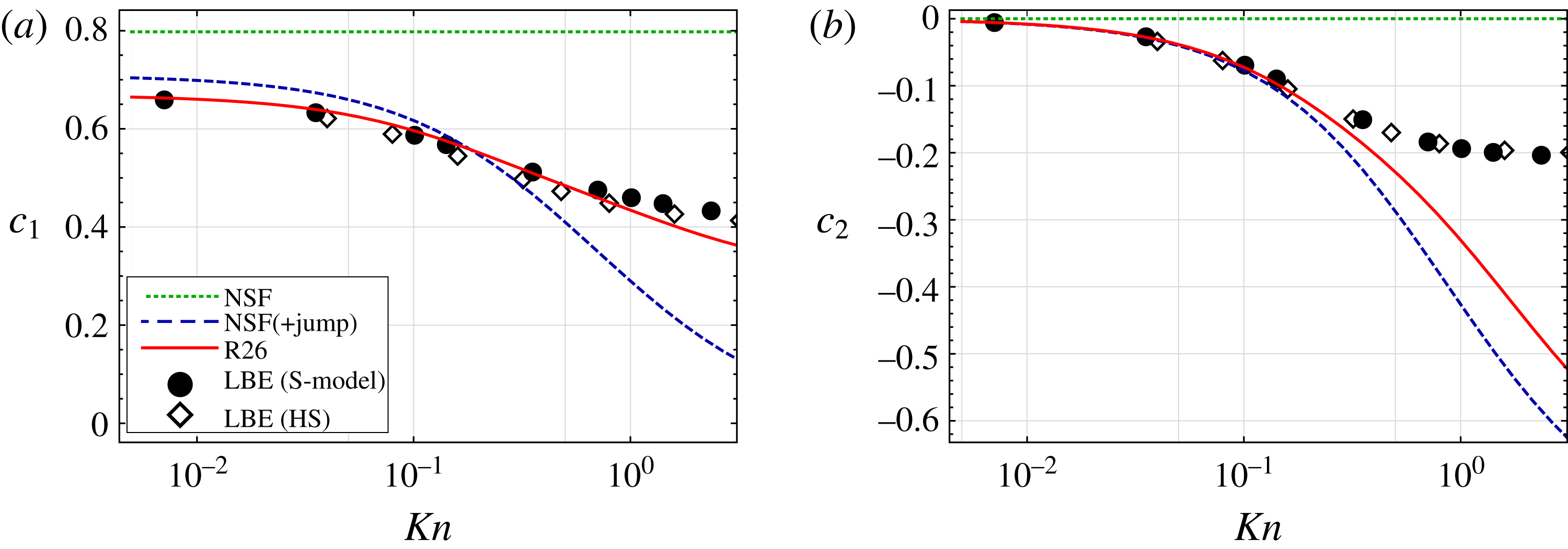
The LHKS relation (5.6) used for NSF gives a constant mass flow coefficient for all Knudsen numbers, as shown in figure 5(a). The LHKS relation is derived for a planar interface; therefore, it does not take the curvature of the interface into account. Furthermore, the heat-flux coefficient is zero (figure 5
b) for the NSF model, which follows from the no temperature jump condition at the interface. Consequently, the NSF model is insensitive to variations in
 $Kn$
and loses validity for microflows. On the other hand, the NSF(+jump) model includes the temperature jump and the curvature effects, and gives a non-constant mass flux and non-zero heat flux, with an offset of approximately
 $10\,\%$
for
 $Kn\lesssim 0.4$
in mass-flux coefficient and
 $Kn\lesssim 0.1$
in heat-flux coefficient.
As illustrated in figure 5, the R26 results for
 $c_{1}$
are within
 $10$
% of kinetic data for
 $Kn\lesssim$
3 (figure 5
a), while for
 $c_{2}$
they are valid for
 $Kn\lesssim$
 $0.5$
(figure 5
b).
8.2 Temperature-driven flow
$(p_{l}=0,\unicode[STIX]{x1D703}_{l}=1)$

In this case, figure 6 shows that
 $c_{1}<0$
and
 $c_{2}>0$
; that is, a mass flux from vapour to liquid (condensation) and a positive heat flux from liquid are induced. This flow behaviour is governed by the boundary conditions (5.3a
) and (5.3b
). For
 $\unicode[STIX]{x1D703}_{l}>0$
, the heat goes from liquid to vapour giving
 $c_{2}>0$
from the boundary condition (5.3b
); therefore the mass-flux equation (5.3b
) leads to condensation at the interface, i.e.
 $c_{1}<0$
.
Mass flow coefficient
 $c_{1}=vr^{2}$
and (b) heat-flux coefficient
 $c_{2}=qr^{2}$
as a function of the Knudsen number for the temperature-driven case (
 $p_{l}=0$
,
 $\unicode[STIX]{x1D703}_{l}=1$
). The symbols, circles and diamonds, denote the results obtained in Chernyak & Margilevskiy (Reference Chernyak and Margilevskiy1989) and Takata et al. (Reference Takata, Sone, Lhuilliere and Wakabayashi1998), respectively, from the linearised Boltzmann equation.
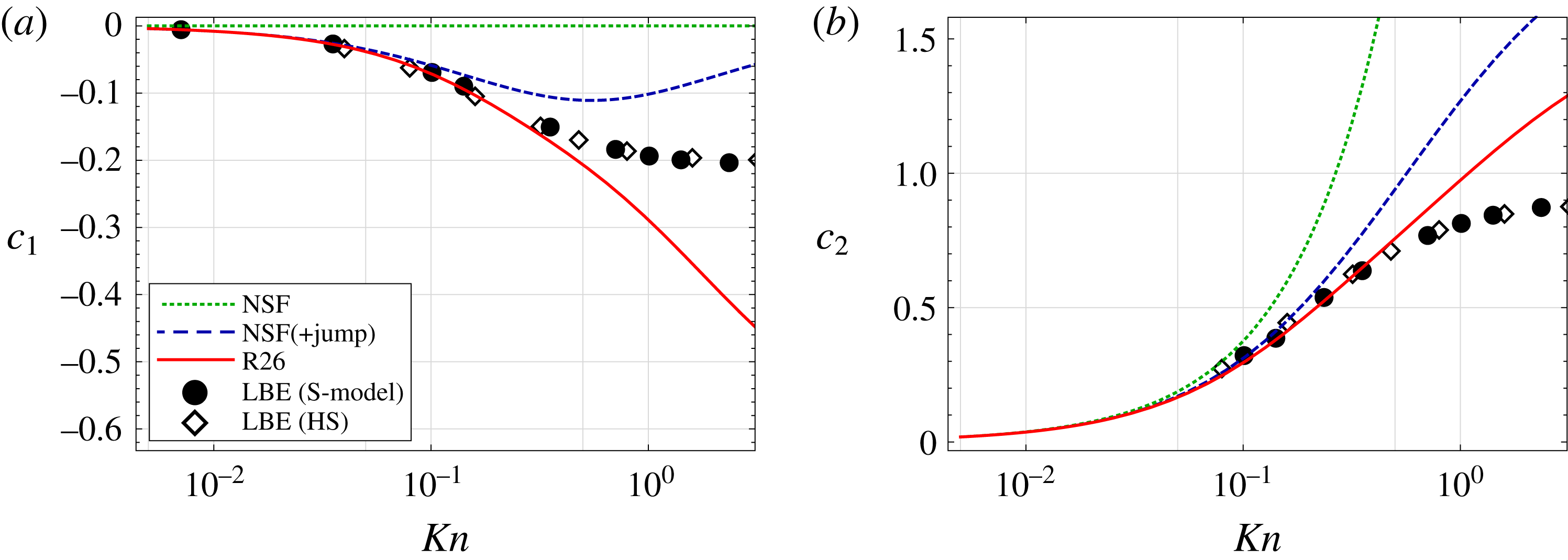
From figure 6(a,b), it can be seen that all models agree well with the LBE simulations for small
 $Kn$
, but in both cases the R26 model shows considerable improvement over the NSF-based models at moderate
 $Kn$
. The R26 results are within
 $10$
% of kinetic data for
 $Kn\lesssim 0.8$
for both
 $c_{1}$
and
 $c_{2}$
, while the NSF(+jump) model shows similar agreement for
 $Kn\lesssim 0.3$
.
8.3 Onsager reciprocity relations
Due to the microscopic reversibility of the evaporation and condensation processes, the Onsager reciprocity relations should hold (Xu et al.
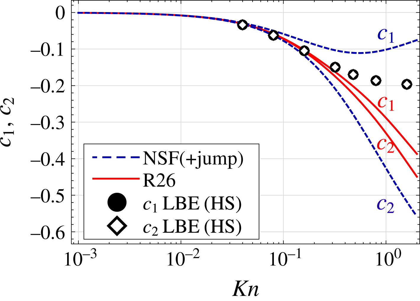
Reference Xu, Kjelstrup, Bedeaux, Rsjorde and Rekvig2006), which in this case state that the heat-flux coefficient (
 $c_{2}$
) driven by the pressure difference should be equal to the mass flow coefficient (
 $c_{1}$
) driven by the temperature difference. In figure 7, our theoretical results for the heat-flux coefficient in the pressure-driven case and the mass flow coefficient in the temperature-driven case are compared to kinetic data from Takata et al. (Reference Takata, Sone, Lhuilliere and Wakabayashi1998). As shown, in the kinetic simulations Onsager reciprocity relations are valid for the entire range of Knudsen numbers. On the other hand, macroscopic theories derived here give agreement extending up to
 $Kn\lesssim 0.5$
for R26 and
 $Kn\lesssim 0.03$
for NSF(+jump), with approximately 10 % deviation. Note that for the classical NSF both
 $c_{1}$
and
 $c_{2}$
vanish. Therefore, within the range which we expect R26 to be accurate, Onsager reciprocity is approximately satisfied.
It has been shown by Rana & Struchtrup (Reference Rana and Struchtrup2016) that the macroscopic wall boundary conditions, derived using Grad’s closure at the boundary, violate the reciprocity relation for high Knudsen numbers. Violation of the reciprocity relation is a serious concern for macroscopic boundary conditions; therefore, a more careful study of the thermodynamically admissible boundary conditions based on a full second law analysis with proper Onsager coefficients is required, which is beyond the scope of this paper. However, as observed in Rana & Struchtrup (Reference Rana and Struchtrup2016), the evaporation/condensation boundary conditions derived here should allow us to identify and estimate the values of the unknown coefficients appearing in such thermodynamically admissible boundary conditions.
Validity of Onsager’s reciprocity relation,
 $c_{2}(p_{l}=1,\unicode[STIX]{x1D703}_{l}=0)=c_{1}(p_{l}=0,\unicode[STIX]{x1D703}_{l}=1)$
, is examined for NSF with jump boundary conditions (dashed blue lines) and R26 equations (solid red lines). Our analytic solutions for MM over moderate Knudsen numbers are compared to LBE kinetic data symbols from Takata et al. (Reference Takata, Sone, Lhuilliere and Wakabayashi1998). The LBE solutions for
 $c_{1}$
and
 $c_{2}$
(symbols) coincide.
To summarise our findings in § 8, it has been shown in this section that the classical NSF model fails to even qualitatively describe LBE results. The R26 model shows significant quantitative improvements over the popular NSF(+jump) approach and, impressively, is within 10 % of all LBE data for
 $Kn\lesssim 1$
as compared to
 $Kn\lesssim 0.1$
for NSF(+jump). With respect to practical computations of microflows, this means the R26 theory can be relied upon for an order of magnitude smaller characteristic scales than the NSF(+jump) theory.
9 Non-Newtonian total normal stress
Having an analytic solution allows us to analyse the magnitude of competing contributions to this non-equilibrium flow. Here we study the total normal stress (
 $p+\unicode[STIX]{x1D70E}$
) experienced by the liquid droplet, whose sign will be seen to change depending on which theory is used. Our primary focus is to understand how this happens by studying the competing contributions from the Newtonian stress, thermal stress and stress due to the Knudsen layer, as defined in § 4.3.
Total normal stress (
 $p+\unicode[STIX]{x1D70E}$
) for (a) pressure-driven case and (b) temperature-driven case for
 $Kn=0.1$
. The solid (red) curves show the R26 solutions, the NSF(+jump) solutions are denoted by the dashed (blue) curves and the NSF with the classical boundary conditions without temperature jump are depicted by dotted (green) curves.
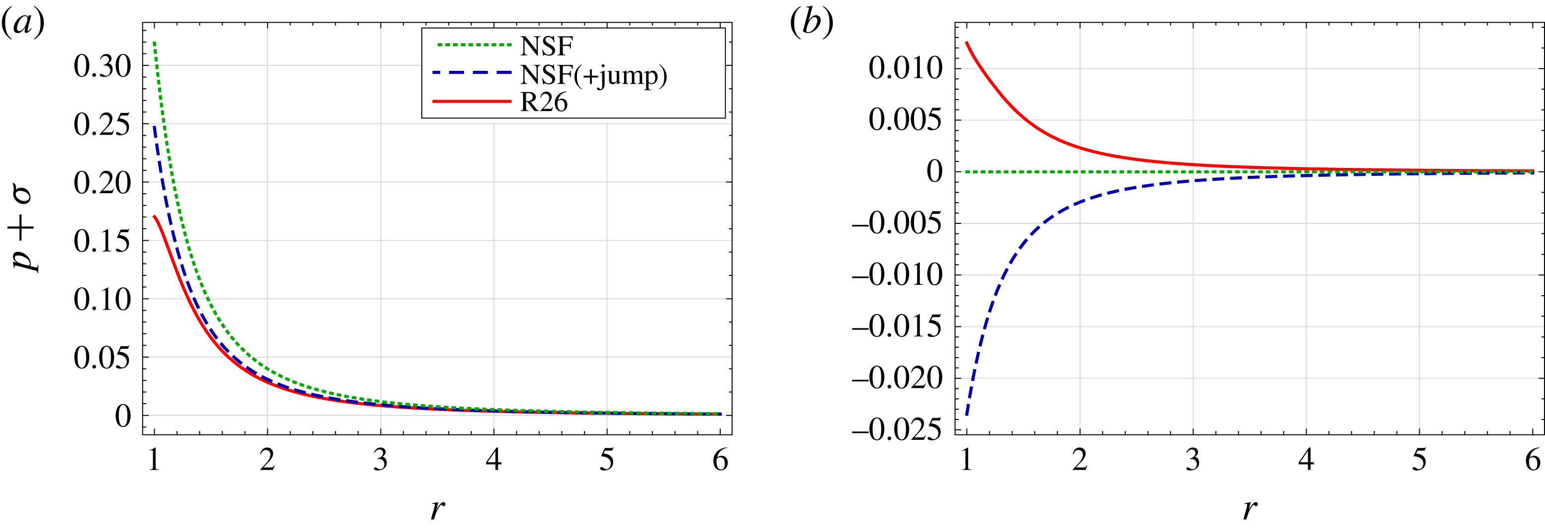
Figure 8 shows the total normal stress obtained from three macroscopic models (NSF, NSF(+jump) and R26) for the pressure-driven case (figure 8
a) and the temperature-driven case (figure 8
b). The results evaluated are for a relatively small Knudsen number
 $Kn=0.1$
.
In pressure-driven flow (figure 8 a), all data, including the classical NSF theory, predict essentially the same qualitative behaviour: a maximum at the interface and decay to zero in the far field. Nonetheless, there is a substantial gap in case of the classical NSF theory, in particular, near the interface, whereas a somewhat better agreement is observed between the NSF(+jump) and R26 models.
Notably, there is a fundamental difference in case of temperature-driven flow in figure 8(b): the total normal stress is zero for the classical NSF model, negative for the NSF(+jump) model and positive for the R26 model. The ultimate origin of this behaviour can be explained in a concise way by the non-Newtonian contributions to the total normal stress in the R26 theory.
Different contributions to the total normal stress (
 $p+\unicode[STIX]{x1D70E}$
) for (a) pressure-driven case and (b) temperature-driven case obtained from the R26 equations for
 $Kn=0.1$
. The Newtonian stress is denoted by the dot-dashed (grey) curves, thermal stress is denoted by the dashed (green) curves, normal stress due to Knudsen layer are depicted by the dotted (purple) curves and the total normal stress is denoted by the solid (red) curves.
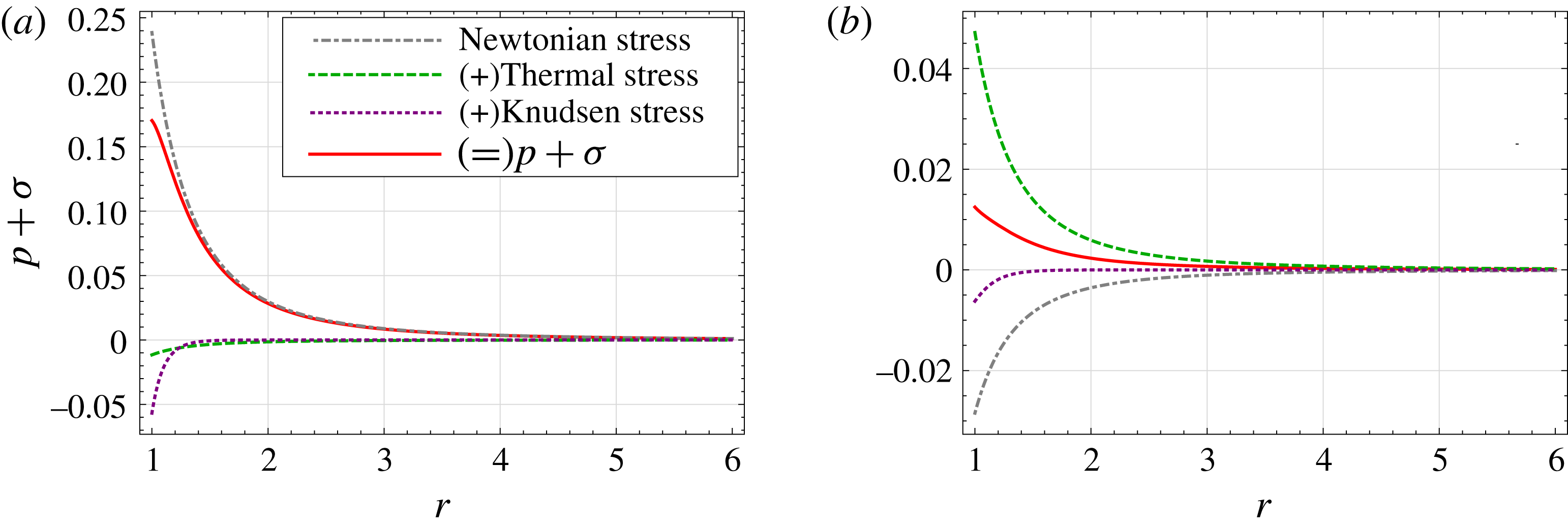
Figure 9 shows the different contributions to the total normal stress for the pressure-driven case (figure 9
a) and the temperature-driven case (figure 9
b) obtained from the R26 equations for
 $Kn=0.1$
. In both of these figures, due to the small
 $Kn$
, the Knudsen layer (denoted by the dotted purple lines) is restricted close to the interface. Furthermore, in both the cases, the thermal stress (dashed green lines) is of second order in Knudsen number, as the term
 $Kn\,c_{2}\sim O(Kn^{2})$
, see § 6.
For the pressure-driven case (figure 9
a), the hydrodynamic stress (denoted by the dot-dashed grey lines) is of first order in
 $Kn$
. Hence, for this case, the thermal stress contribution as is one order of magnitude smaller than the Newtonian stress; so that the total normal stress (solid red lines) away from the interface is dominated by the Newtonian stress.
More interestingly, for the temperature-driven case (figure 9
b), the Newtonian stress is of second order, as
 $Kn\,c_{1}\sim O(Kn^{2})$
, i.e. of the same order as the thermal stress, but, critically, of opposite sign. As a result the thermal stress forces the total stress to become positive whereas without its contribution, as in the NSF, this contribution would be negative.
10 Summary and conclusion
This article has developed the macroscopic modelling of phase-change processes and shown that the R26 equations provide a significant improvement over conventional models, accurately approximating benchmark Boltzmann equation results up to
 $Kn\approx 1$
. Notably, the analytic solutions provide unique insight, by allowing us to decompose our solution and determine the relative contributions of different physical effects, particularly in and around the Knudsen layers.
The R26 equations have been considered for planar wall boundary-value problems, for example in Gu & Emerson (Reference Gu and Emerson2009), Gu et al. (Reference Gu, Emerson and Tang2010), Gu & Emerson (Reference Gu and Emerson2014). However, the analytical solution in a spherical geometry and more importantly for a liquid–vapour phase boundary was attempted for the first time here. Our analytic solution highlights why the R26 model is superior to the R13: it has access to three exponential functions to describe the Knudsen layer rather than just one. These findings are consistent with those of Gu & Emerson (Reference Gu and Emerson2014), where superposition of three exponentials from the R26 theory produced an improved description of the thermal Knudsen layer.
The general interest of the present study is to explore boundary-value problems for moderately rarefied gas flows, with an emphasis on evaporation from nanostructures. For example, evaporative cooling from nano pores
 ${\sim}O(100~\text{nm})$
can lead to thermal management in electrical systems directly at the source of hot spots. Such a device operates around atmospheric pressure, with mean free path
 $\unicode[STIX]{x1D706}\sim O(10~\text{nm})$
(based upon the saturation temperature) in the vapour phase, giving a Knudsen number
 $Kn\lesssim O(1)$
. For the purpose of design optimisation, which requires repetition of simulations with different parameters, Boltzmann solvers can become impractical due to the large computational time involved. Macroscopic models, despite limitations on the their accuracy, give a computationally fast and detailed access to quantities of interest. The R26 theory developed here, which we have benchmarked against LBE, gives us a framework to study evaporation/condensation for
 $Kn\lesssim O(1)$
, i.e. down to nanoscales.
Very recently, fundamental solutions (Green’s functions) were derived for the linearised R13 equations by Claydon et al. (Reference Claydon, Shrestha, Rana, Sprittles and Lockerby2017). The numerical framework based upon these fundamental solutions, generalised to account for phase-change phenomena, should allow for three-dimensional multiphase microflows to be modelled at remarkably low computational cost. Extension of the method of fundamental solutions for the R26 equations and development of a simulation tool for moment equations to capture geometrically complex flows will be the subject of future work.
Another line of inquiry is to study thermodynamically admissible boundary conditions for higher-order moment equations. It has been shown by Rana & Struchtrup (Reference Rana and Struchtrup2016) that the macroscopic boundary conditions, derived using Grad’s closure at the boundary, violate the reciprocity relation for high Knudsen numbers, i.e. there arises the problem of boundary conditions for a finite system of equations that approximate the microscopic boundary conditions for the Boltzmann equation. The boundary conditions must be consistent with the moment equations and the resulting problem must be resolved. Looking forward, a more careful study of the boundary conditions based on a full second law analysis with proper Onsager coefficients should lead to improved agreement between macroscopic theories and exact solutions of the Boltzmann equation.
Acknowledgements
This work has been financially supported in the UK by EPSRC grants (EP/N016602/1, EP/P020887/1 and EP/P031684/1) and the Leverhulme Trust. A.S.R. has also received funding from the European Union’s Horizon 2020 research and innovation programme under the Marie Skodowska-Curie grant agreement no. 713548.
Supplementary material
Supplementary material is available at https://doi.org/10.1017/jfm.2018.85.
Appendix A. Solution for the R26 equations
Here we shall give a step by step procedure to obtain the analytic solution for the R26 equations. As a Step 1 we assume that the pressure is given as the superposition of exponential functions given by (4.7a
). In Step 2, by substituting this ansatz in the momentum balance equation (3.4b
) and integrating, we readily obtain the expression for
 $\unicode[STIX]{x1D70E}$
given in (4.7b
). Step 2 introduces a constant integration
 $b_{1}$
. In Step 3, we shall use the stress balance equation (3.7a
) to get
 $m$
 $$\begin{eqnarray}m=\frac{b_{2}}{r^{4}}-15\mathop{\sum }_{i=1}^{3}a_{i}\left(1+\frac{r\unicode[STIX]{x1D6FE}_{i}}{Kn}+\frac{2r^{2}\unicode[STIX]{x1D6FE}_{i}^{2}}{5Kn^{2}}+\frac{r^{3}\unicode[STIX]{x1D6FE}_{i}^{3}}{15Kn^{3}}\right)\frac{Kn^{4}\text{e}^{-r\unicode[STIX]{x1D6FE}_{i}/Kn}}{r^{4}\unicode[STIX]{x1D6FE}_{i}^{5}},\end{eqnarray}$$
where,
 $b_{2}$
is a new constant of integration. By substituting
 $m$
from the previous equation into (3.10a
), in Step 4, we obtain
 $\unicode[STIX]{x1D6F7}$
. Note that, Step 4 does not introduces any additional integration constants. In Step 5, we substitute
 $\unicode[STIX]{x1D70E}$
,
 $m$
and
 $\unicode[STIX]{x1D6F7}$
, from previous steps into the balance equation for
 $m$
(3.9a
), to obtain
 $R$
. This step brings one new integration constant
 $b_{3}$
, scaling with
 $r^{2}$
, as
 $$\begin{eqnarray}R=b_{3}r^{2}+\frac{1}{r}(\cdot )+\frac{1}{r^{3}}(\cdot )+3\mathop{\sum }_{i=1}^{3}a_{i}\left(1+\frac{r\unicode[STIX]{x1D6FE}_{i}}{Kn}+\frac{r^{2}\unicode[STIX]{x1D6FE}_{i}^{3}}{3Kn^{3}}\right)(\cdot )\frac{\text{e}^{-r\unicode[STIX]{x1D6FE}_{i}/Kn}}{r^{3}\unicode[STIX]{x1D6FE}_{i}^{3}},\end{eqnarray}$$
where, expressions inside the brackets
 $(\cdot )$
do not depend on
 $r$
. For any physically meaningful solutions,
 $R$
must vanish as
 $r\rightarrow \infty$
, therefore
 $b_{3}=0$
. An expression for
 $\unicode[STIX]{x1D713}$
is obtained from the equation (3.10b
) in Step 6. In Step 7,
 $\unicode[STIX]{x1D714}$
is obtained from the balance equation for
 $R$
(3.9b
), which again gives an integration constant
 $b_{4}$
scaling with
 $r$
, therefore
 $b_{4}=0$
. At this point, in Step 8, we have to obtain a solution for
 $\unicode[STIX]{x1D6E5}$
which satisfies equation (3.9c
) and equation (3.10c
), at the same time. We get
 $\unicode[STIX]{x1D6E5}$
from (3.9c
) and substitute
 $\unicode[STIX]{x1D714}$
,
 $\unicode[STIX]{x1D6E5}$
and
 $R$
in (3.10c
) to get
 $$\begin{eqnarray}\displaystyle & \displaystyle b_{1}={\textstyle \frac{4}{5}}(5c_{1}+2c_{2})Kn, & \displaystyle\end{eqnarray}$$
 $$\begin{eqnarray}\displaystyle & \displaystyle b_{2}=\left(\frac{2c_{2}}{5Pr_{M}Pr_{R}}+\frac{5c_{1}+2c_{2}}{5Pr_{M}}\right)36Kn^{2}, & \displaystyle\end{eqnarray}$$
 $\unicode[STIX]{x1D6FE}$
as
 $$\begin{eqnarray}\displaystyle 120374\unicode[STIX]{x1D6FE}^{6}-242756\unicode[STIX]{x1D6FE}^{4}+119400\unicode[STIX]{x1D6FE}^{2}-1\,5306.4 & = & \displaystyle 0,\end{eqnarray}$$
for the MM model, and
 $$\begin{eqnarray}\displaystyle 81081\unicode[STIX]{x1D6FE}^{6}-110055\unicode[STIX]{x1D6FE}^{4}+37905\unicode[STIX]{x1D6FE}^{2}-3675 & = & \displaystyle 0,\end{eqnarray}$$
for the BGK model. The positive roots of these polynomials were listed in table 1. Finally, the expression for the temperature
 $\unicode[STIX]{x1D703}$
is obtained by substituting
 $\unicode[STIX]{x1D6E5}$
,
 $R$
,
 $\unicode[STIX]{x1D70E}$
and
 $q$
into (3.7b
) and then solving for
 $\unicode[STIX]{x1D703}$
. The new constant
 $c_{3}$
following from this integration vanishes due to (4.4).
The coefficients
 $k_{1}$
,
 $k_{2}$
and
 $k_{3}$
appearing in (4.8) depend on the transport coefficients in the collision model and are given by
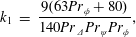 $$\begin{eqnarray}\displaystyle k_{1} & = & \displaystyle \frac{9(63Pr_{\unicode[STIX]{x1D719}}+80)}{140Pr_{\unicode[STIX]{x1D6E5}}Pr_{\unicode[STIX]{x1D713}}Pr_{\unicode[STIX]{x1D719}}},\end{eqnarray}$$
 $$\begin{eqnarray}\displaystyle k_{2} & = & \displaystyle -\frac{81Pr_{M}Pr_{\unicode[STIX]{x1D719}}+Pr_{\unicode[STIX]{x1D713}}(64Pr_{\unicode[STIX]{x1D6E5}}+9Pr_{\unicode[STIX]{x1D719}}(4Pr_{\unicode[STIX]{x1D6E5}}+7Pr_{R}+2)+80Pr_{R})}{36Pr_{\unicode[STIX]{x1D6E5}}Pr_{\unicode[STIX]{x1D713}}Pr_{\unicode[STIX]{x1D719}}},\end{eqnarray}$$
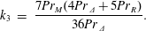 $$\begin{eqnarray}\displaystyle k_{3} & = & \displaystyle \frac{7Pr_{M}(4Pr_{\unicode[STIX]{x1D6E5}}+5Pr_{R})}{36Pr_{\unicode[STIX]{x1D6E5}}}.\end{eqnarray}$$


 Open access

