Introduction
A geophysical and glaciological program to study the West Antarctic ice streams that drain into the Ross Ice Shelf was begun in 1983, with initial studies on Ice Stream B. Upstream B (UpB) camp, in the middle of Ice Stream B2, one of the main branches of Ice Stream B (Fig. 1), was established in November 1983.
a. Antarctica, showing the resistivity stations discussed in the text (reproduced from Reference BentleyDrewry (1983) with modification). b. Map of West Antarctic Ice Streams A, B and C showing the location of UpB camp). Hachured strips denote zones of concentrated crevasses. The short-dashed line indicates the grounding line (junction with the Ross Ice Shelf). The long-dashed line shows the boundaries between two ice streams. For more detail, see Shabtaie and Reference Alley and BentleyBentley (1988).

Geophysical experiments conducted at and near UpB during the 1983-84 season included electrical resistivity sounding. Previous resistivity measurements at station RI, located in the flow band of Ice Stream E on the Ross Ice Shelf (Reference BentleyBentley, 1976; Reference Shabtaie and BentleyShabtaie and Bentley, 1979, Reference Shabtaie and Bentley1984), had revealed the existence of highly resistive ice at the base of the ice shelf with resistivity comparable to that reported for temperate glaciers (e.g. sec Röthlisberger and Reference Shabtaie and BentleyVögtli, 1967; Reference Glen and ParenGlen and Paren, 1975). Resistivity measurements were conducted on Ice Stream B particularly to obtain more information about the nature of this anomaly. Electrode separations covered a large enough range (2 m 3 km) to study the ice stream throughout its thickness.
The field methods, data analysis and modeling techniques are similar to those previously described (Reference BentleyBentley, 1977; Reference Shabtaie and BentleyShabtaic and Bentley, 1979, Reference Shabtaie and BentleyShabtaic and Bentley 1984, in press a); we will not discuss them here. Here, we first calculate the resistivity as a function of depth in the ice, ρ(z), to be expected from the variations of temperature and density. Then, we calculate the corresponding apparent resistivities, ρa, and find that they do not match the observations well. We find that we must introduce additional parameters, representing other physical and chemical changes in the ice, to find a satisfactorily fitting model.
Measurements of density and temperature
Density
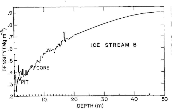
Densities were measured on a 21 m core that was extracted at UpB camp near the resistivity profile during the 1983–84 field season. Cores were cut into pieces 10-20 cm long, and the densities (Fig. 2) were calculated by measuring the length, diameter and the weight of the individual pieces. To measure densities in the uppermost layers, density-tube samples were taken from the side walls of a 2.5 m pit at different depths and weighed. Each plotted density (Fig. 2) tram the pit is the mean of four measurements at each depth. For densities at depths greater than 21m, we have taken a smooth curve through spot measurements on a 100m core from a hole drilled near the center of the resistivity profile during the 1984-85 field program (Reference Alley and BentleyAlley and Bentley, 1988).
Density versus depth at UpB. The 1983-84 pit and core densities are indicated. The smooth curve at depths greater than 20 m shows mean densities from the 1984–85corehole

Temperatures
Temperature measurements were made in the pit and the 21 m corehole on 16 and 17 January, just before and after the resistivity measurements. Temperatures in the pit were read from pre-installed thermometers; those in the 21 m corehole were measured at intervals of 0.5-1 m using a Thermometric glass thermistor sensor. The temperature profile (Fig. 3a) shows the expected mid-summer shape.
a. Temperature versus depth at UpB. a. Temperatures in the upper 20 m measured in the pit and shallow corehole at UpB. b. Temperatures from two different hot water drilled holes. Crosses show the measurements in the 1983–84 200 m hole circles show measurement, in a hole drilled to the bed (Personal communication from H. Engelhardt, 1993). The solid line is the temperature model described in the text.
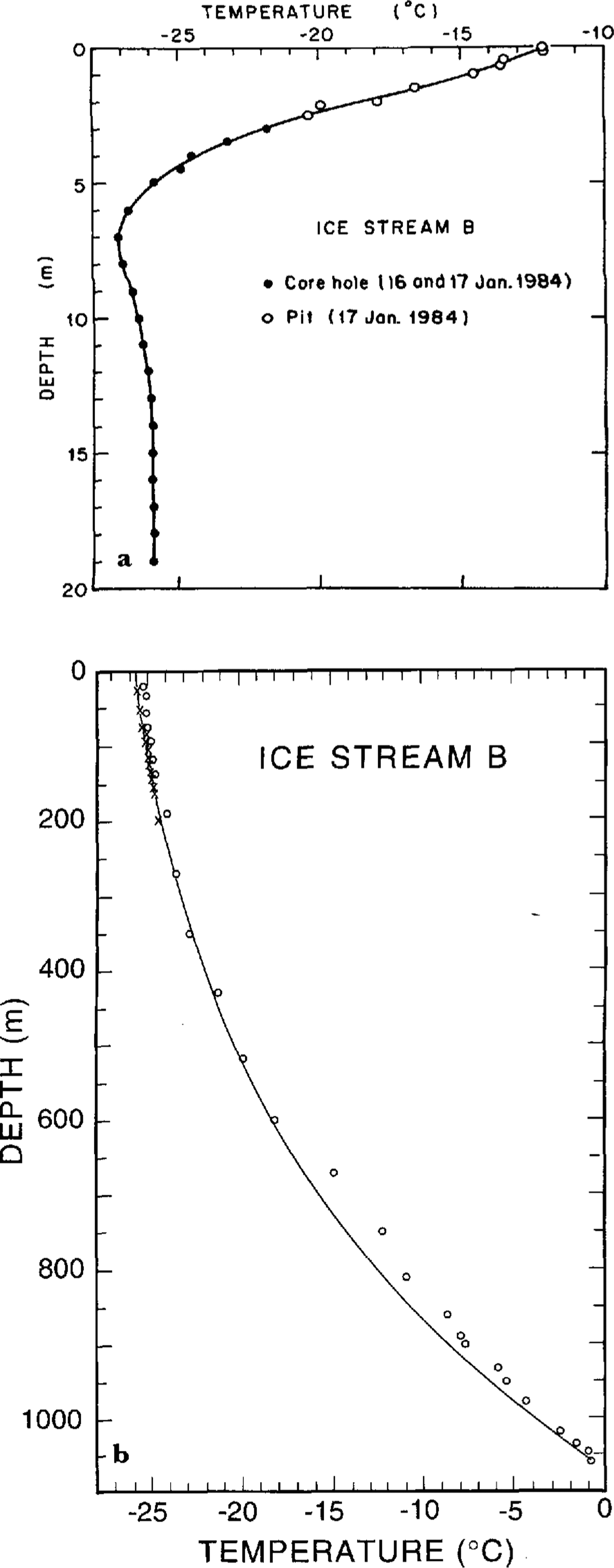
During December 1983, a string of 15 thermistor sensors was emplaced at depths between 25 and 200 min a hot-water drillhole. Temperature measurements (Fig. 3b) were made in January 1985, 13 months after the installation of the sensors (long enough to eliminate transient temperature changes). The temperatures show no negative gradient below the winter cold wave in the upper 10 m, which implies that the advection of cold ice from upstream is insignificant.
Temperatures deeper than 200 m were calculated from the model discussed next.
Temperature modeling
Basal boundary condition
The temperature gradient, Gg, that would be produced at the base of a stationary ice sheet by the geothermal flux, qg, in the absence of melting is

where θc (7 x 10⁷Jm 1 a-1°C-1) is the thermal conductivity of ice. For moving ice, the contribution from basal shear heating must be added to the geothermal heat to obtain the basal temperature gradient, Gb; then, still with no melting,

where τb is basal shear stress and Vb is the sliding velocity. (The shear-heating term in (Equation 2) is independent of how the basal shear stress is accommodated by the ice sheet and its bed, so long as the heat is released near the interface.) We assume that the basal shear stress is equal to the driving stress,τ and that Vb, is equal to surface velocity, V. These assumptions maximize both τb and Vb and therefore maximize our calculated rate of strain heating. The driving stress is given by

where is the mean ice-column density, g is the acceleration of gravity, H is the ice thickness and is the surface slope averaged over a distance of 20H to eliminate the effect of longitudinal stress gradients.
At Byrd Station, the assumption of a negligible basal melt rate is acceptable. The value of Gb measured in the corehole there was 0.0325°C m-1 (Reference Gow, Ueda and GarfieldGow and others, 1968) and also τbVb/θc = 0.0065" C m-1 (Reference Budd, Jenssen and RadokBudd and others, 1971). (Equation 2) then gives Gg = 0.026°C m -1. This is close to the value of Gg, 0.023°cm-1, given by (Equation 1) for a global mean geothermal flux of 1.6 × 10⁶Jm-2 a1. Lacking any better value, we initially assume Gg = 0.026°C m1 also at UpB.
For an ice stream, the basal melt rate, bH, is not negligible, so (Equation 2) is not valid; instead,

where L (335 J g-1) is the specific latent energy of fusion and γi (0.917 Mg m-3 is the density of ice. (Equation 4) is a simple generalization of an equation given by Reference Whillans, Bolzan and ShabtaicWeertman (1961). Gb and bH arc both unknown and cannot be estimated independently, so we treat bH as an adjustable parameter in the heat equation. At UpB, V = 440 ma-1 (Reference Shabtaie, Whillans and BentleyWhillans and others, 1987), H = 1060 m,α = 2.4 x 10⁻³ (Reference Shabtaie and BentleyShabtaie and others, 1987) and γi = 0.90 (calculated from Figure 2); then τb = τ = 22kPa, from (Equation 3).
Ice-stream temperature model
The equation of heat conduction in an ice sheet is (see Reference PatersonPaterson, 1981, chapter 10):

where T is the temperature, t is time, θd is the thermal diffusivity, z is the vertical direction (positive downward), X is the horizontal direction along the flow, y is the horizontal direction transverse to flow, W is the vertical velocity of an ice particle, ėxy and τxy arc the xy components of strain rate and shear stress, respectively, and C is the specific-heat capacity of the ice. In solving Equation, we assume: (a) the firn layer can be ignored, (b) horizontal temperature gradients are negligible and internal strain heatings are small compared with the basal shear heating. Furthermore, we can neglect the horizontal advection term (∂T/∂x) at UpB, because there is such a small regional difference in mean annual 10m temperatures (-26° to -27°C, 300 km downstream of UpB on the ice shelf (Reference VögtliThomas, 1976) compared with -24° to -26°C, 200-300 km upstream (Reference Bentley, Cameron, Bull, Kojima and GowBentley and others, 1964)) and because, as already mentioned, our temperature measurements (Fig. 3b) show that advection is not significant.
The vertical velocity (W) can be approximated by (Reference Whillans, Bolzan and ShabtaicWeertman, 1961)

where is the surface balance rate (9 cm ice a-1 at UpB (Reference Shabtaie and BentleyShabtaie and Bentley, 1987). The temperature at the bed is given by the pressure-melting temperature, Tm, which can be found from the Clausius Clapeyron relationship (Reference RobinRobin, 1976) Tm≈µP, where = µ=-7.4 × 10⁴°C m2 N-1 and is the hydrostatic pressure. For UpB, Tm = -0.7°C.
(Equation 5) can be solved numerically for steady state (∂T/∂t=0). Our procedure was to assume different values of bH, from which Gb and W could be calculated from Equations and (6), respectively. The modeled temperature-depth curves were then matched against the measured temperatures in the upper 200 m of the ice stream. We found for the best-fitting model bH = 0.07 m a-1 (the fit worsens markedly outside the range of 0.05<bH<0.1) and Gb = 0.05°Cm-1 (Fig. 3b). The modeled melt rate is twice that, 0.032 m a-1, generated by the shear-heating term in (Equation 4), even though that value is an upper limit. That could indicate an elevated geothermal flux or other unrecognized heat source, or it could reflect a violation of the assumption of steady state or of assumptions (b) or (c), all of which are questionable for such a high-energy system as an ice stream. For resistivity modeling, fortunately, why T(z) has a particular shape is irrelevant.
Recent deep drilling at UpB has made it possible to obtain temperatures all the way to the bed (Reference Engelhardt, Humphrey, Kamb and FahnestockEngelhardt and others, 1990). The latest measurements (personal communication from H. Engelhardt, 1993) are plotted in Figure 3b. There is satisfactory agreement for our purposes between modeled and measured temperatures, although there is a slight offset between them deeper than 600 m and the measured basal temperatures show fluctuations larger than would be expected so deep in the ice sheet. We have not deemed it fruitful to re-do our -resistivity modeling on the basis of the measured temperatures, as we are concerned with effects far larger than those caused by the small temperature differences.
Resistivity
In an ice sheet, density, temperature, impurities, crystal size and other chemical and physical properties change with depth and can or might affect the resistivity. The two parameters whose effects upon ρ(z) are known are those whose determination we have already discussed, temperature and density. We will try to evaluate the effects of other factors from the measured resistivities.
The effect of temperature on the resistivity of both firn and solid ice is governed by the Arrhenius law with activation energy E:

where ρ0 = ρ(0) is the resistivity of the surface layer with temperature T0 = TK(0), k = 8.6 × 10⁻⁵ eV K-1] (Boltzmann's constant) and TK is the absolute temperature. An activation energy of 0.25 eV for firn and solid ice was determined from resistivity and temperature measurements at Dome C, on the East Antarctic plateau (Shabtaie and Bentley, in press a). That value also works well at UpB, as is shown by the modeling discussed below.
Firn can be modeled as a mixture of two components, ice and air, with volume fractions ν1 and ν2 where ν1 + ν2 = 1. The mixture equation derived by Reference LooyengaLooyenga (1965) describes the electrical behavior of firn well. In general, Looyenga's equation gives the complex permittivity of a mixture, in terms of two component permittivities ε1 and ε2:

Equation 8 is symmetrical in ν2 and ν1, i.e. the result is the same regardless of whether the mixture is assumed to be ice in air or air in ice. For the d.c. limit, (Equation 8) reduces to

where σ is the d.c. conductivity. For firn, σ = σfirn, σ1 = σice, σ2 = σair = 0 and ν2 = 1 – ν1 = 1 - γfirn/γice, where γfirn and γice are firn and ice densities, respectively.The resulting mixture equation for the resistivity of firn is

Reference BentleyBentley (1977) and Reference Shabtaie and BentleyShabtaie and Bentley (1979, in press b) found that (Equation 10) closely described resistivities measured at several stations on the Ross lee Shelf and at Dome C.
Bed resistivity
Another parameter needed for calculating Pa is the resistivity in the bed. The resistivity of wet, porous sediments, ρr, is generally approximated by Archie's law (Reference ArchieArchie, 1942):

where ρw is the pore-water resistivity, a ~ 1 and m. ~ 1.5 for most sedimentary rocks, and Φ is the porosity. The resistivity we need is the mean resistivity of the upper few hundred meters of the subglacial sediments. Seismic work (Reference Rooney, Blankenship, Alley, Bentley, Thomson, Crame, Thomson, thlisberger and gtliRooney and others, 1991) indicates that 60Ωm of low velocity (~2 kms-l) sediment underlies the ice at UpB, so no deeper layers need be considered. The wave velocity implies a porosity of about 30% (Reference Blankenship, Bentley, Rooney and AlleyBlankenship and others, 1987). Using a typical ground-water resistivity of 10Ω m (Reference Shabtaie and BentleyShabtaie and others, 1987) leads to a resistivity of only 60Ω. Measurement between two probes 20 m apart in the bed at UpB, however, suggested a resistivity greater than 100Ω m (personal communication from H. Reference Engelhardt, Humphrey, Kamb and FahnestockEngelhardt, 1990). To be conservative, we take a high resistivity value for modeling purposes (1000Ω m, except where otherwise noted) ― adoption of a lower value would only strengthen our conclusion that the basal ice has high resistivity.
Apparent resistivity models
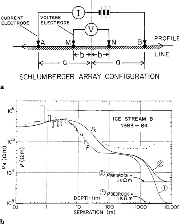
From the data presented in Figures 2 and Figure 3, and (Equations 7) and (10), we can calculate what ρ(z) would be if it depended on γ and T alone (Fig. 4). In our numerical model, the layer thicknesses range from 0.1m at the top of the ice sheet to 10m at the bottom. For model 1, ρbedrock = l kΩm, and E = 0.25eV. The corresponding model for Pa, the apparent resistivity calculated by the numerical techniques discussed by Shabtaie and Bentley (in press a), is also shown in Figure 4. The ρa model fits the data for a <40 m but falls much lower than the data at greater separations. This is still true even when resistivity as high as 5 kΩm (pure subglacial melt water (Reference GowGow, 1968)) in the bed is assumed (Fig. 4, model 2). I t is clear that the cause of the high resistivity anomaly is not a high value of the bed resistivity, so we will use a value of 1 kΩ m for the remainder of this analysis.
a.Schlumberger four-electrode array configuration; a and b are the current and potential electrode separations (i.e. distance from the center), respectively. The apparent resistivity ρa for this configuration is given by 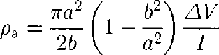 where ∆V and I are potential difference and current, respectively. b. Plots of apparent resistivity, ρa, versus electrode separation and modeled resistivity, ρ, versus depth. The heights of the data-point symbols represent the standard deviations of the measurements. The two models show the effects of temperature and density only, with different assumed resistivities in the bed. The vertical and horizontal scales are the same for both ρa and ρ.
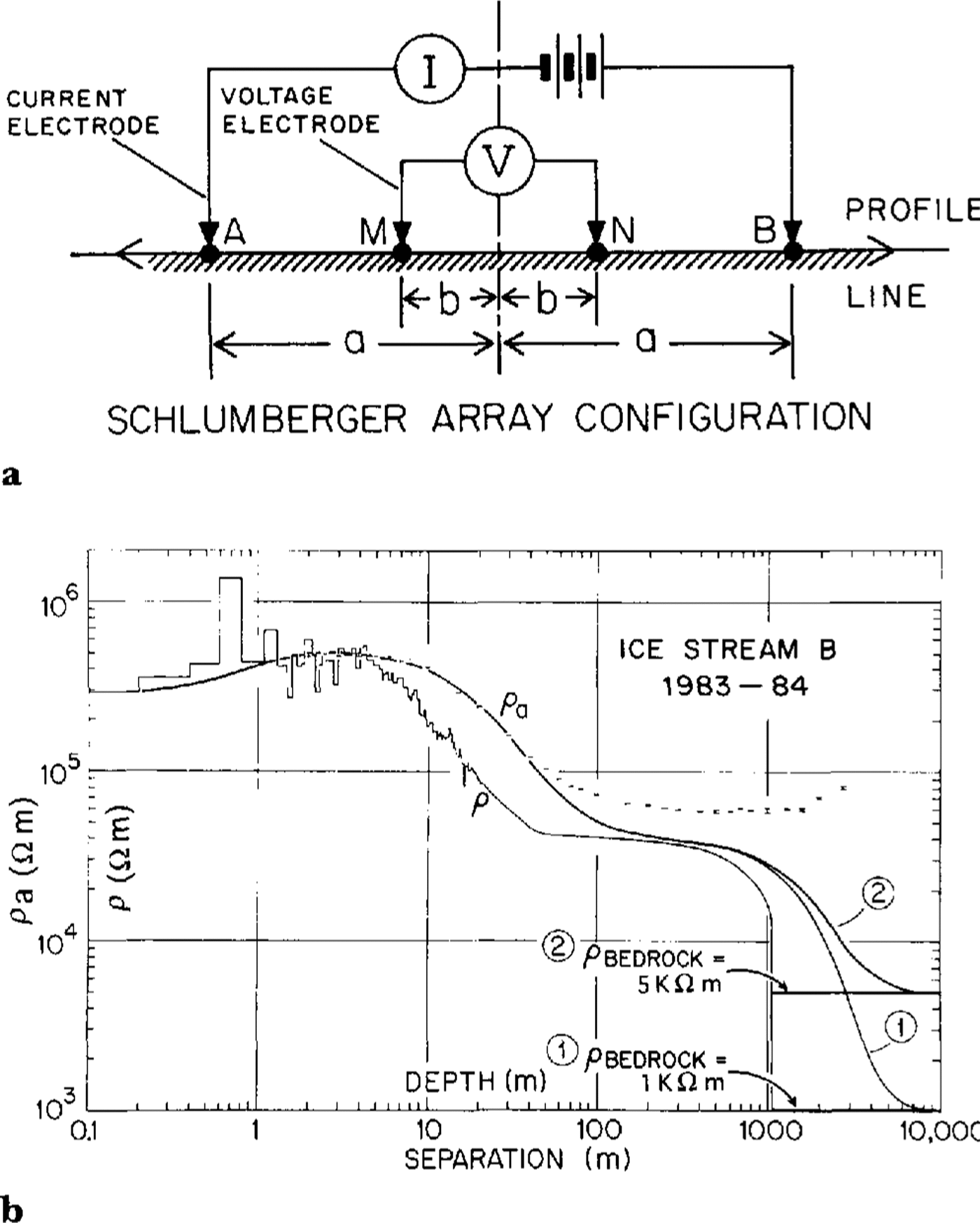
Several models that incorporate high resistivity anomalies (in addition to the temperature and density effects) were tested; a few examples are shown in Figures 5 and Figure 6. The fact that modeled and measured ρa differ for a>40 indicates that the high resistivity must start at a shallow depth. I t is clear from model 3 (Fig. 5) that a gradual increase starting at a shallow depth will not work. What is required is an increase in ρ(z) by a factor of about 1½, starting at about 20 m (Fig. 5, models 4 and 5).
Plot, of modeled resistivity versus depth (dashed lines) and corresponding apparent resistivity versus electrode separation (solid lines) for models 3, 4 and 5. Model1 is repeated for reference. Dots are the apparent resistivity data points; the diameter of the dots is equal to the largest standard deviation (the point at a = 1000 m in 10,000 Figure 4). Note the different scales for ρa and ρ

An increase by several orders of magnitude in ρ(z) deep in the ice is needed to produce the high ρa values at large separations. Models that include such an increase below 800 m fit the data fairly well (Fig. 5, model 5; Fig. 6, model 6) but a still better fit is provided by a model in which ρ(z) first decreases to a lesser value between 650 and 800 m (Fig. 6, models 7 and 8). Model 8 fits the data particularly well. Comparison of models 7 and 8 shows the sensitivity of the models changes in the position of the peak and trough in ρ(z) between 650 and 800 m depth.
Plots of modeled resistivity versus depth (dashed lines) and corresponding apparent resistivity versus electrode separation (solid lines) for models 6, 7 and 8. Model 1 is repeated for difference. Dots are the apparent resistivity data points; the diameter of the dots is equal to the largest standard deviation (the point at a = 1000 m in Figure 4). Note the different scales for ρa and ρ.

The shape of the best-fitting model (Fig. 6, model 8) is similar to the one calculated for other stations in Antarctica. Resistivity depth curves from several sites (R I, near the mouth of Ice Stream E on the Ross Ice Shelf; J9, also on the ice shelf (Shabtaie and Reference Shabtaie and BentleyBentley, 1984, in press a)) are shown along with our model for Ice Stream B in Figure 7. In general, the profiles show similar features; exceptions are the sharp increase in p(z) at shallow depth on the UpB profile and the absence atJ9 of the order-of-magnitude increase in the basal ice.
Best fitting models of resistivity (or conductivity) versus depth, corrected to solid-ice density and a temperature of – 20° C, at four Antarctic locations.

The analyses for station J9 (Reference Shabtaie and BentleyShabtaie and Bentley, 1984) and Dome C (Shabtaie and Bentley, in press a) show that variation of ρ(z) with depth does not correlate with salts, sulfates, acids or any other impurities found in the chemical analysis of ice cores from those sites. Instead, changes in ρ(z) are highly correlated with crystal-size variation. For example, at Dome C both resistivity and crystal-size increase between 90 and 400 m, and below 540 m; in between, in the Holocene Wisconsin transition zone, both decrease markedly. This correlation is also found elsewhere (Reference Shabtaie and BentleyShabtaie and Bentley, 1984). Furthermore, the shape of ρ(z) at UpB correlates well with crystal-size variation at Byrd Station (Reference Gow and WilliamsonGow and Williamson, 1976). By analogy, therefore, we conclude that the Wisconsin-Holocene transition zone at UpB is at a depth between 6.50 and 800 m.
Electrical conductivity behavior of polar ice
It has long been known that resistivities In polar ice sheets are two or three orders of magnitude lower than in temperate and laboratory ice (see Reference Glen and ParenGlen and Paren, 1975; Reference BentleyBentley, 1977; Reference Shabtaie and BentleyShabtaie and Bentley, 1979, Reference Shabtaie and BentleyShabtaie and Bentley 1984). The resistivities we have obtained from measurements at 13 locations on the East and west Antarctic inland ice and on the Ross Ice Shelf (SReference Shabtaie and Bentleyhabtaie and Bentley, 1979; work in progress by S. Shabtaie) and measurements elsewhere in the Arctic and Antarctic (Reference Meyer and thlisbergerNleyer and Röthlisberger, 1962; Reference østremøstrem, 1967; Reference Glen and ParenGlen and Paren, 1975) all show this for the upper layers of the ice sheet. In deep polar ice, however, in both East and west Antarctica, the range of the resistivity values is close to that of temperate ice, although the temperatures are well below freezing.
Reference Fitzgerald and ParenFitzgerald and Paren (1975) found that the electrical behavior of polar ice samples changed after melting and refreezing to that of temperate or pure ice. Reference Glen, Homer and ParenGlen and others (1977) proposed that temperate glaciers are purified by the flushing out of interstitial impurities by percolating melt water. But phenomena that require melting cannot explain high resistivities in deep polar ice that has always been frozen. Furthermore, field measurements both in the Arctic (Reference Wagenbach, Münnich, Schotterer and OeschgerVogtli, 1967) and in the Antarctic (Reference ReynoldsReynolds, 1982), in zones where there is surface melting and refreezing, yielded resistivities that are typical of polar ice rather than temperate ice.
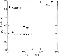
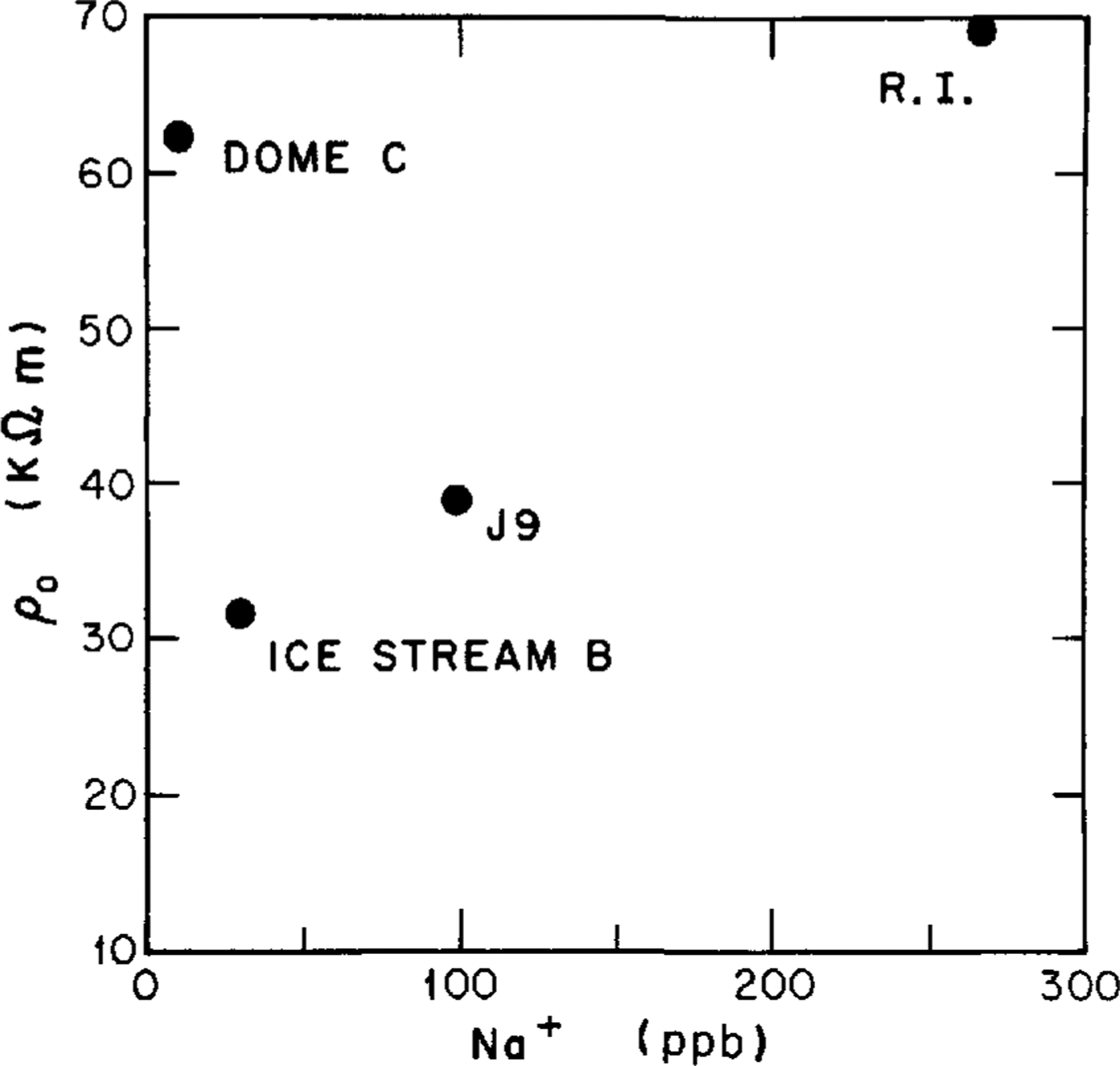
It is possible that soluble impurities are incorporated substitutionally into the ice lattice and that the concentration of these impurities affects the defect population, thus changing the resistivity of the ice. Laboratory measurements on monoerystalline ice doped with HF, HCI and NaCl (Reference Camplin, Glen and ParenCamplin and others, 1978; Reference Gross, Hayslip and HoyGross and others, 1978) have shown resistivities comparable with those in polar ice. However, the required impurity concentrations are much higher than the levels found in polar-ice samples: 8-.50 μM of HF (Reference Camplin, Glen and ParenCamplin and others, 1978) and 3-40 μM of HCI or NaCl (Reference Gross, Hayslip and HoyGross and others, 1978) compared with impurity levels in polar ice sheets that range from less than 1-3 μM (Reference Delmas, Ascencio and LegrandDelmas and others, 1980; Reference Petit, Briat and Royer Petit and others, 1981; Reference HerronHerron, 1982; Reference Legrand and DelmasLegrand and Delmas, 1988). Furthermore, there is no correlation between measured near-surface resistivities (corrected to solid-ice density and 20°C and salt concentration in the form of Na + (Reference Boutron and LoriusBoutron and Lorius, 1977; Reference Herron and LangwayHerron and Langway, 1979) for our Antarctic sites (Fig. 8). Resistivity modeling based on measured variations of salt impurities with depth at J9 (Reference Shabtaie and BentleyShabtaie and Bentley, 1984) and Dome C (Reference Shabtaie and BentleyShabtaie and Bentley, in press a) also failed to match the measured values. Although measurements in a few deep holes in both the Arctic and the Antarctic confirm the existence of impurities throughout the ice column, the impurity concentrations in temperate glaciers, which are found relatively close to industrial centers and/or deserts, are up to an order of magnitude larger than in polar ice (Reference WeertmanWagenbach and others, 1988). Clearly, the cause of the very low conductivities in temperate and some polar ice cannot be related to impurities alone; some other factor or factors must come into play.
Near-surface resistivity, corrected to solid-ice density and a temperature of -20° C, versus salt concentration at four Antarctic stations.
New model
At several locations, we have observed a strong correlation between conductivities and crystal size (Reference Shabtaie and BentleyShabtaie and Bentley, 1984, in press a). An explanation for this is found in a theoretical model (unpublished work of S. Shabtaie) in which the impurities surround the ice grains like shells. The impurity coatings must already exist at very shallow depth to explain electrical conduction in near-surface low-density snow (Reference Shabtaie and BentleyShabtaie and Bentley, 1990, in Reference Shabtaie, Whillans and Bentleypress b).
Near the surface, the grains are about 1 mm2 in size and are ellipsoidal in shape. However, both melting and deformation at high stresses cause extensive recrystallization and crystal growth in the ice. In temperate glaciers and deep in polar ice sheets, crystals can reach over 100 cm2 in size and are no longer convex in shape; they twist, fold and surround other crystals and become "interlocking" (Reference RigsbyRigsby, 1968; Reference GowGow, 1970). In our model, this transformation and recrystallization effectively breaks the continuity of the impurity shells surrounding the ice crystals - it is the connectivity of the system that controls the conduction. Breaking the conducting paths does not mean removing the impurities from the system, only disconnecting them. Moderate concentrations of impurities in temperate ice and deep polar ice are accommodated by locating them in isolated domains at grain boundaries.
We believe this new model can explain conduction phenomena throughout an ice sheet. Quantitative details have been worked out for snow and firn by Reference Shabtaie and BentleyShabtaie and Bentley (in press a) and for solid ice in a manuscript soon to be submitted.
Conclusions
A detailed resistivity profile was completed on Ice Stream B at separations from 2 m to 3 km. Resistivities were modeled as a function of depth using measured densities and temperatures, and functional relations that are now well known. Fits were good only in the uppermost part of the ice sheet; below that, model fitting required a 50% increase in resistivity at a depth of only about 20 m and an increase by at least two orders of magnitude in the bottom 200 m or so. A five-fold decrease in resistivity between 650 and 850 m was also suggested; by analogy, we associate this with the Holocene-Wisconsin transition zone. We propose that the principal features of the resistivity- depth profile can be explained by the degree of connectedness between impurities lying on two-grain boundaries. In particular, we believe that the high resistivity at large depth arises because the extensive recrystallization and grain growth at those depths destroy the connectivity of the two-grain-boundary conduction paths.
Acknowledgements
Special thanks are due to PICO personnel (B. Koci, J. Anderson and B. Boller), who drilled the 200 m hot water hole. Other individuals who assisted with different aspects of the experiment are J. Dollman, K. C. Taylor, B. R. Weertman and J. E. Nyquist. The field program was supported by U.S. National Science Foundation grant DPP-81-20332. This is contribution 546 of the Geophysical and Polar Research Center, University of Wisconsin-Madison.