I. INTRODUCTION
A survey into spectrum utilization within the 30 MHz–3 GHz band revealed that licensed frequency bands are underutilized. On the contrary, unlicensed bands experience high percentage utilization [Reference Cordeiro, Challapali, Birru and Sai Shankar1]. This led to the development of cognitive radios (CRs). CRs will opportunistically utilize these underutilized frequency bands. The promise of wide instantaneous bandwidth has made CR an active research area. CR nodes are wireless devices that are aware of their surroundings and can adjust their operating parameters autonomously [Reference Harada2]. CRs can be said to originate from software defined radios (SDRs). Jondral [Reference Jondral3] and Haykin [Reference Haykin4] describe CRs as SDRs that can additionally sense their environment, track changes, and react to the findings. With the definitions in [Reference Jondral3, Reference Haykin4], it is clear that one of the key requirements of CR nodes is spectrum sensing. It is a key requirement because the nodes have to detect any licensed user, also called a primary user (PU), as quickly as possible after the PU becomes active. For example, IEEE802.22 specifies a limit of two seconds [Reference Cordeiro, Challapali, Birru and Sai Shankar1].
There have been numerous discussions about how best to prevent CR nodes from causing harmful interference to PUs. One of the suggestions involves creating a database of free spectrum in which CR nodes will have real time access to, hence removing the need for spectrum sensing capability in every CR node. This is a reasonable idea but there is still a need for spectrum sensing at central locations to update the database. This scheme best suites a fully established network of CR nodes but does not suite CR nodes that intend to form or are in ad-hoc networks [Reference Fette5] and CR nodes would still need to detect each other.
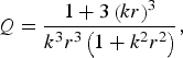
Wideband antennas or wide tuning antennas are required to carry out spectrum sensing. Wideband antennas are preferable because they give the opportunity to utilize the advances made in concurrent baseband signal processing with digital signal processing (DSP). Current social trends suggest that CR nodes would ultimately be handheld and mobile. This means that antennas are of limited dimensions and hence electrically small and narrowband. Additional techniques are required to make this antenna broadband. The trade-off between antenna size and Q imposed by the Chu limits makes realizing this antenna difficult. The relationship between Q and antenna size, defined by the radius r of the smallest sphere that can enclose the antenna, is given in (1) [Reference Schantz6].
 $$Q=\displaystyle{{1+3\left({kr} \right)^3 } \over {k^3 r^3 \left({1+k^2 r^2 } \right)}}\comma$$
where, k = 2π/λ.
Passive matching networks help to match antennas, but because they involve resonating the reactive part of the antenna with passive elements, they only give good match at specific frequencies. Away from this spot frequency, the antenna return loss decreases. This necessitates the use of multiple or reconfigurable matching networks to cover wide frequency bands.
However, using non-Foster elements could help provide continuous wideband matching because unlike Foster elements, the slope of the reactance versus frequency of a non-Foster element is always negative. This means that the locus on the Smith chart goes in the anticlockwise direction with increasing frequency. With these properties, non-Foster elements are able to cancel out completely the reactance of other elements and antennas because of the difference in slope and direction of rotation on the Smith chart. Typically, non-Foster elements are negative capacitors and inductors.
II. NEGATIVE IMPEDANCE CONVERTER
A) Linvill circuit
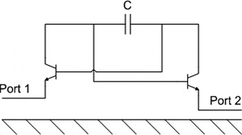
One means of achieving non-Foster elements is through the use of negative impedance converters (NIC). NICs were first proposed by Linvill [Reference Linvill7]. Sussman-Fort and Rudish [Reference Sussman-Fort and Rudish8] described the NIC as a two port network which generates the negative of whatever impedance is connected across one port. The negative impedance is seen across the second port. The Linvill NIC consists of two transistors connected in the common base configuration. The reactance to invert is connected between the two collectors and the base of one transistor is connected to the collector of the second transistor in the form of a feedback path. The emitters form the two ports of the NIC. The circuit schematic of the NIC is shown in Fig. 1. Note that the schematic does not include the bias network.
Linvill's NIC circuit schematic.

Prior work on NICs includes reference [Reference Sussman-Fort and Rudish8], in which a NIC was realized with a top frequency of 120 MHz. The NIC was used to match a 6 and 12 inch blade antenna. Its performance in terms of signal-to-noise (S/N) over a resistively matched antenna and gain were shown. It performed better than a passively matched equivalent over a wide bandwidth. The paper also showed better performance than a resistive matched blade antenna. In [Reference Mirzaei and Eleftheriades9], the NIC was used to match a meta-material antenna. A NIC was used along with trimming capacitors to obtain a relatively wideband tuneable match. Its top frequency was at 500 MHz with the bandwidth match of 200 MHz. Other publications [Reference Aberle10–Reference Song and Rojas14] all show simulated performance of the NIC. One of the reasons why NICs have not been achieved in the higher frequency ranges is because of the difficulty involved in achieving a stable NIC. As the frequency is increased, the complexities involved in realizing the NIC increase because of the parasitics of the components used. One of the major challenges of the NIC design is stability though it is reciprocal and symmetrical. Standard stability test methods such as the K factor, auxiliary stability factor (B1) test, and the position of stability circles do not correctly predict the instabilities experienced with NICs. This is a position also shared by Stearns [Reference Stearns15].
B) Antenna and simulation result
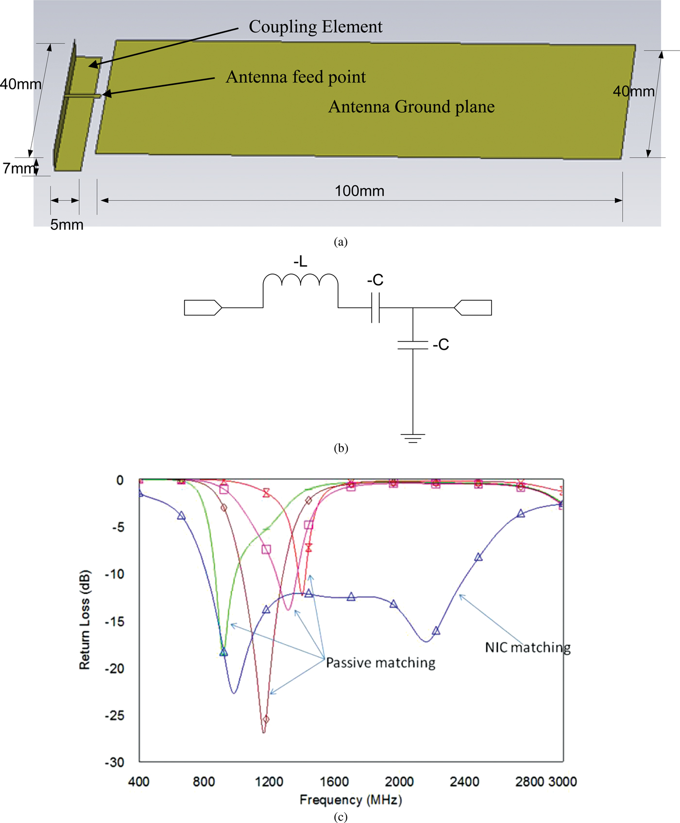
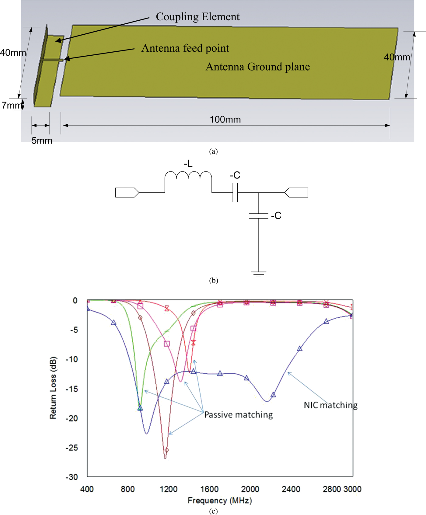
The antenna used in this work is a chassis antenna. The coupling element is displaced from the edge of the ground plane which also doubles as the radiating element. It can also serve as the chassis of a mobile or handheld device. The dimensions of the ground plane are 40 mm × 100 mm. The size of the coupling element is 40 mm × 5 mm × 7 mm and it is displaced from the edge of the ground plane by 6 mm. The ground plane and coupling elements are fabricated from copper. They are held together by RohacellTM with ɛr of 1.08. Extensive work has been done on this antenna as reported in [Reference Hu, Kelly, Song, Hall and Gardner16]. A physical representation is shown in Fig. 2(a). The Q of the antenna is found to be 19 at 900 MHz. Negative elements realized by simulating Linvill's circuit schematic with an AVAGO ATF54143 transistor were used to match this antenna and wideband matching was achieved. The L-shaped matching network, shown in Fig. 2(b), consists of negative capacitors and inductors. The series negative inductor and capacitor were simulated using one NIC circuit and the shunt element was simulated using another NIC circuit. A detailed schematic of this matching network and its performance can be found in [Reference Tade, Hu, Gardner and Hall17–Reference Tade, Gardner and Hall18]. The non-Foster matching network provided an antenna return loss of −10 dB or better between 800 MHz and 2.4 GHz as shown in Fig. 2(c). This achieved a Q of 0.94. Realizing this Q with passive matching is not possible because of the Chu Limit. To cover this same bandwidth would require switching between multiple matching networks as can be seen in Fig. 2c, where the best effort results of matching the antenna with passive matching network are shown. It can be noted that narrow band are obtained and multiple networks are required to cover an 800 MHz bandwidth.
(a) The antenna structure. (b) The three negative element matching network. (c) Simulated NIC matched antenna return loss compared with best effort passive matching.
To start off, it was decided to first fabricate a single negative element using the Linvill's NIC model. The initial attempt at fabrication using the ATF 54143 transistor resulted in a circuit that was unstable with oscillation at 2.4 GHz. This instability and oscillations were not evident when stability checks were performed using the K factor and B1 auxiliary stability factor.
III. STABILITY ANALYSIS
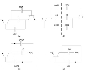
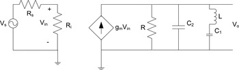
The standard stability test, K factor and B1 auxiliary stability factor test, for two port networks may fail to reveal instability. This is because they rely on a test done through two ports and these would not show instabilities due to the hidden modes. An approximate analytical stability method has been developed which is based on the transfer function analysis [Reference Sedra and Smith19]. Figure 3(a) shows the NIC schematic for a single negative element. The capacitor to invert is C and CB1 and CB2 are the DC blocking capacitors required in the NIC. In even mode, the current out of the transistors into the capacitor to invert, C, are equal but opposite in the direction of flow. This means that an open circuit is formed in the middle of the capacitor and effectively removes the influence of the capacitor in the analysis. The currents around the feedback paths are also equal but the direction of flow is the same, as shown in Fig. 3(a). Taking advantage of the symmetry of the circuit, the circuit can be split into two along its line of vertical symmetry (Fig. 3(b); this makes the value of the capacitors in the feedback path 2CB1 each and the capacitor to invert becomes 2C. Figure 3(c) shows one-half of the split circuit. Taking into consideration the current flow directions, it is possible to close-up the circuit and form Fig. 3(d). This then forms the basis of the rest of the analysis. The capacitors 2CB1 and 2CB2 are added together and this yields C 1 in Fig. 3(d). The equivalent circuit of the transistor and C 1 in Fig. 3(d) is shown in Fig. 4.
(a) The NIC schematic. (b) NIC in even mode operation. (c) NIC after split along its line of symmetry. (d) NIC with closed-up feedback path.

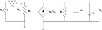
Equivalent circuit for even mode NIC without feedback path.

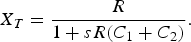
X T is the parallel combination of R, C 2 and C 1.
 $$X_T = \displaystyle{R \over {1 + sR\lpar C_1 + C_2 \rpar }}.$$
Now,
 $$V_0 = g_m V_{in} X_T \comma$$
so that
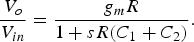 $$\displaystyle{{V_o } \over {V_{in} }} = \displaystyle{{g_m R} \over {1 + sR\lpar C_1 + C_2 \rpar }}.$$
The pole of this transfer function is:
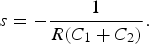 $$s = - \displaystyle{1 \over {R\lpar C_1 + C_2 \rpar }}.$$
It can be seen that the poles will be real and on the left side of the S-plane. This implies that the circuit will be unconditionally stable. The NIC schematic consists of a feedback path and this would be realized with transmission lines. The transmission lines which form the feedback path can be represented approximately by inductors. The inductance values are calculated from the line lengths. If this inductor, the equivalent of the feedback path between the two transistors, is included in series with the capacitor C 1 (Fig. 5) in the analysis, the circuit equivalent and transfer function becomes (6)
 $$\displaystyle{{V_o } \over {V_{in} }} = \displaystyle{{g_m R\lpar 1 + s^2 LC_1 \rpar } \over {s^3 RLC_1 C_2 + s^2 LC_1 + sR\lpar C_1 + C_2 \rpar + 1}}.$$
Equivalent circuit for even mode NIC with feedback path.

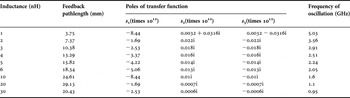
Typical values of R and C 2 can be obtained from the data sheet of the transistor (Avago ATF 54143). L is the inductor which approximately represents the circuit board track in the feedback path and C 1 is the DC blocking capacitor. Using these values, the positions of the poles of the transfer function can be determined. The poles of this transfer function are:
 $$s_1 = - 4.1166 \times 10^{12}\comma \;$$
 $$s_2 = 0.0142i \times 10^{12} \comma \;$$
 $$s_3 = - 0.0142i \times 10^{12} \comma \;$$
(R = 0.3 Ω, L = 4.9 nH, C 1 = 1 pF and C 2 = 0.8 pF).
Because they are on the imaginary axis of the s-plane and are complex conjugates, the circuit will oscillate at a given frequency with fixed amplitude. The frequency of oscillation was found to be at 2.26 GHz which is within 5% of the measured frequency of oscillation. Table 1 shows the results of a parametric study on the feedback path length using the analysis above. This shows how the frequency of oscillation changes with changes to the feedback length represented by inductance values. This gives a means of achieving a stable NIC that works at higher frequency ranges. It should be noted that the inductances are only approximations and as the length of the feedback path increases, the level of approximation increases.
Parametric analysis of NIC stability.

The stability analysis and the parametric study not only shows that reducing the length of the feedback path length helps achieve a stable NIC at higher frequency but it shows at what frequency the structure will become unstable for a given feedback path length. This is very useful as it helps in the choice of transistor used with every given structure. The transistor is chosen to ensure that its transition frequency is lower than the predicted frequency of oscillation given the length of the feedback path in the particular structure.
IV. NIC REALIZATION
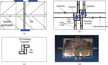
Using the information harnessed from the stability analysis in Section III, a NIC has been designed and built with a top frequency of 1.5 GHz which is the highest reported so far. In order to make the feedback path as small as possible, it was decided to design the NIC as a double layered structure. The top frequency is limited to 1.5 GHz by the choice of the transistor. With the feedback path length of 15 mm, the expected frequency of oscillation, calculated using the method in Section III, is 2.4 GHz. A transistor with a transition frequency of 1.5 GHz was therefore chosen, to give a reasonable margin. The structure is 50 × 50 mm with a common ground plane in between, Fig. 6(a). The two layers are connected together through a via. The top layer (Fig. 6(b)) contains the two transistors, the capacitor to invert and the DC bias network. The feedback path and the DC blocking capacitors are on the bottom layer, Fig. 6(c). The transistors used are SOT-23 package NXP BFS-17 transistors with a transition frequency (F T) of 1.5 GHz, which are biased at 5 V, 20 mA. The capacitor to invert is an AVX 3.9 pF capacitor. The substrate is Taconic TLY-5 with ɛr 2.2 and tan δ of 0.0009.
NIC layout: (a) cross-sectional view, (b) top view, (c) reverse view and (d) built NIC.

Negative elements are inherently unstable [Reference Sussman-Fort and Rudish8]; hence to measure the structure, there is a need to add passive elements so that the net reactance seen from the two measurement ports are positive. The actual NIC performance is then de-embedded from the measured results. Points A and B in Fig. 6(b) are the actual terminals of the NIC. Additional coplanar waveguide (CPW) transmission lines of length 17.5 mm are added between points A and B to allow SMA connectors to be used as the measurement ports. There are also 2 pF capacitors in shunt between the measurement ports and points A and B to make the overall capacitance positive and 10 Ω resistors which provide resistive damping. De-embedding is done using the NEG2 element in AWR design environment. A circuit board containing the added positive elements and the CPW transmission line between the measurement port and the points A and B in the circuit (Fig. 6(b)) was built and measured. The measured s-parameters were then fed into the NEG2 block. The NEG2 block in AWR works by negating the transpose of the Y matrix of the network. The NEG2 block was then connected in series at both ends with the s-parameter block of the measured structure. The resultant s-parameters of the cascaded blocks are the de-embedded s-parameters of the NIC. The condition for validity of the NEG2 element approach is met, because the negated network consisting of the CPW transmission lines and the positive lumped element is reciprocal.
A) Measured result
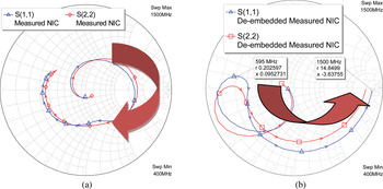
The structure described has been built (Fig. 6(d)) and measured. Figure 7(a) shows the S(1,1) and S(2,2) of the measured structure before de-embedding. It should be noted that the locus around the Smith chart is still clockwise, which represents Foster elements. This is because of the additional elements between the measurement port and points A and B (Fig. 6(b)). When the effects of these elements have been de-embedded, Fig. 7(b) is obtained. This exhibits the expected non-Foster performance by its anticlockwise rotation around the Smith chart with increasing frequency between 0.595 GHz and 1.5 GHz. The graph of impedance seen from the two ports against frequency has been reported in [Reference Tade, Gardner and Hall20]. It shows a negative slope with an increasing frequency which is characteristic of non-Foster elements.
Measured NIC (a) before de-embedding and (b) after de-embedding.

B) NIC matching
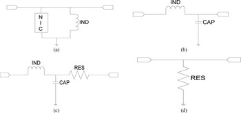
Owing to the complexity involved in achieving the NIC described above, the three element matching network was revised. Instead of using the three negative elements matching network, a new matching network which is made up of the single element NIC and a positive inductor was designed, Fig. 8(a). In this case, the measured de-embedded NIC was combined with an inductor. To obtain the best performance, the matching network needs to be as close to the antenna feed point as possible. We combined the measured de-embedded s-parameters of the NIC, the lumped inductor and the measured antenna in CST and simulated the antenna return loss. The revised matching network and the antenna return loss are shown in Figs 8(a) and 9.
(a) Revised NIC matching network. (b) Reactive passive matching network. (c) Lossy reactive passive matching network. (d) Resistive matching network.

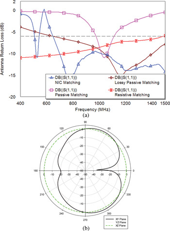
A better than −6 dB return loss was obtained between 647 and 1500 MHz. This shows a better performance than what is obtainable through the use of passive matching networks which shows a −6 dB return loss bandwidth of 137 MHz. The Q of the antenna is reduced from 19 to 1.25 with the NIC matching network. This wide bandwidth and size enables the antenna to be used for spectrum sensing in mobile/handheld devices.
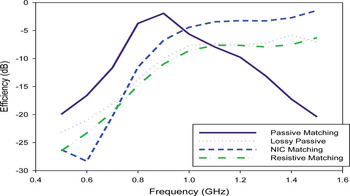
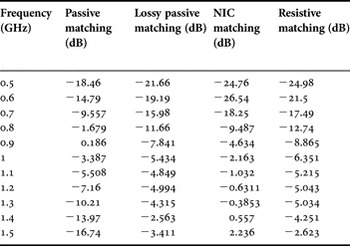
The NIC matching network was compared with other known forms of obtaining wideband return loss in antennas which includes passive matching (Fig. 8(b)), lossy passive matching (Fig. 8(c)), and resistive matching network (Fig. 8(d)). The comparison between the antenna return loss is shown in Fig. 9. There is a portion of the NIC matched antenna return loss that is greater than 0 dB, this is because the input impedance has a small negative resistance of −0.49 Ω at this frequency (508 MHz). This would not start an oscillation as it is small when compared to the system impedance. The antenna return loss of the different matching networks show that resistive matching and lossy matching can also provide wideband matching. The simulated antenna radiation pattern at 1.5 GHz with the revised NIC matching network is shown in Fig. 9(b) in the XZ, XY, and YZ plane and the table showing the gain of the antenna with different matching network is also shown in Table 2. Detailed description of the performance of the different matching networks can be found in [Reference Tade, Gardner and Hall21]. The antenna return loss alone does not give a complete picture as loss is known to also improve return loss. To get the complete picture on the performance of the NIC matched antenna when compared with other matching network alternatives, there is a need to look at the antenna efficiency, Fig. 10. It shows that the NIC matched antenna has a better efficiency when compared to resistive matching and lossy matching which offer wideband performance. It should be noted that the passive match does better over narrower bandwidth.
(a) Antenna return loss with different matching networks. (b) Simulated radiation pattern at 1.5 GHz.

Simulated antenna efficiency with different matching networks.

Simulated gain of the different matching networks.

V. NOISE AND LINEARITY
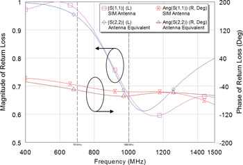
This section describes measurements to establish the noise and linearity performance of the NIC and antenna combination. It has been difficult to fabricate a complete NIC matched chassis antenna majorly because the current fabrication method requires that a large part of the ground plane, about 20%, be used for a single element NIC. Realizing the complete matching network described in Section II would require a sizable amount of the ground plane, which might not be available in practical devices. The ground plane, which also doubles as the radiating element of the antenna, will be disturbed to make accommodation for the NIC and its required biasing network. This disruption disturbs the surface current on the antenna ground plane and causes the impedance of the antenna to change. For practical and commercial fabrication, other methods of fabrication are recommended such as monolithic microwave integrated circuit (MMIC). Owing to this constraint, it was decided to replace the antenna with an equivalent lumped element circuit to allow an assessment of the noise and linearity properties. The antenna equivalent consists of CPW transmission lines and lumped elements and is designed to represent the antenna in the frequency ranges 0.7–1 GHz. This small frequency range was chosen because it is hard to find a practical passive lumped element equivalent for an antenna which completely represents the antenna at over a wider bandwidth. Figure 11 shows the magnitude and phase plots of both the measured antenna and the antenna equivalent circuit. It can be seen that there is a reasonable agreement between the equivalent circuit and the antenna between 700 and 1000 MHz. Below and above this frequency band the frequency response of the equivalent antenna circuit and the actual antenna begin to have significant differences. Hence, the antenna equivalent cannot be used as a true representative of the antenna outside this frequency range. Therefore, the decision was made to characterize the noise and linearity performance of the NIC matched antenna within this frequency range.
Two port equivalent characteristics compared with chassis antenna.

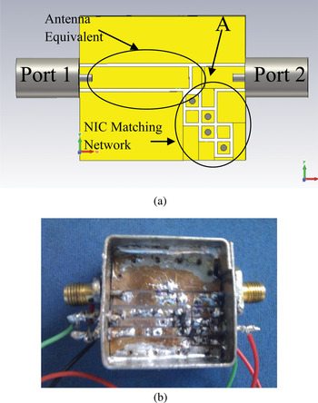
The equivalent circuit transforms the 50 Ω port impedance through transmission lines and lumped elements into the impedance seen at the feed point of the chassis antenna at point A in Fig. 12(a). The NIC matching network is then connected to point A, as shown in Fig. 12(a). Figure 12(b) shows the fabricated NIC matching network with the equivalent circuit representing the antenna.
Equivalent antenna with NIC matching network (a) layout structure and (b) fabricated structure.

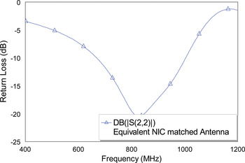
Connecting the NIC matching network to point A is equivalent to having the NIC matching network connected directly to the antenna. Using the same design technique used to realize the NIC in Section IV, the equivalent NIC matched chassis antenna was designed between 0.7 and 1 GHz. The structure is shown in Fig. 12 while its s(2,2) which represents the return loss is shown in Fig. 13. It shows a better than −10 dB return loss within the band of interest.
Measured return loss of equivalent antenna with NIC matching network.

This structure is then used to measure the noise and inter modulation characteristics of the NIC matched antenna.
A) Noise measurement
In order to measure the noise contribution of the representative NIC matched antenna, the Y-factor method [22] was used. In this measurement setup, a Noise Com Inc noise tube (NC346B) with a known excess noise ratio (ENR) was connected to port 1 of the device under test (DUT), which in this case is the equivalent chassis antenna circuit. Port 2 of the DUT is connected to the spectrum analyzer via a low noise amplifier (LNA). The LNA is optional and it is only required to amplify the measured noise power beyond the noise floor of the spectrum analyzer. The noise contribution of the LNA is corrected for in the overall measurement.
The noise tube requires a 28 V supply and by turning this on and off the power levels of both the on and off states N ON and N OFF are recorded. The Y-factor is given by:
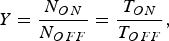 $$Y = \displaystyle{{N_{ON} } \over {N_{OFF} }} = \displaystyle{{T_{ON} } \over {T_{OFF} }}\comma$$
Where T ON and T OFF are given by
 $$T_{ON} = T_{sys} + T_{ON}^s\comma$$
 $$T_{OFF} = T_{sys} + T_{OFF}^s\comma$$
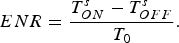 $$ENR = \displaystyle{{T_{ON}^s - T_{OFF}^s } \over {T_0 }}.$$
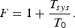
T 0 is the reference temperature or the room temperature during measurements. The ENR in equation (10) is the ENR of the noise tube at the specified frequency. T sys is the noise temperature of the measurement system. T ONs and T OFFs are the noise temperature of the noise tube in its on and off states respectively.
The noise factor of the system F, is computed from the noise temperature by using equation (11),
 $$F = 1 + \displaystyle{{T_{sys} } \over {T_0 }}.$$
The noise factor of the DUT has to be extracted from the measured noise factor of the system by performing a second stage correction using the Friis formula for noise factor,
 $$F_{cascade} = F_1 + \sum\nolimits_{i = 2}^n {\displaystyle{{F_i - 1} \over {G_1 G_2 \cdots G_{i - 1} }}}\comma$$
 $$NF\lpar dB\rpar = 10\log F.$$
Noise figure (NF) of the DUT is then used to calculate the SNR advantage of the NIC matched antenna compared to a lossy matching of the same antenna. The SNR adv is computed using:
 $$SNR_{adv} = \lpar S_{NIC} - S_{lossy} \rpar - \lpar NF_{NIC} - NF_{lossy}\rpar .$$
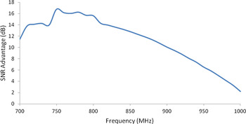
S NIC and S lossy are the gain of the antenna with the different matching networks. Figure 14 shows a SNR advantage of 4 dB or more across the measured frequency band of 700–1000 MHz. It was decided to compare the SNR of the NIC with a lossy matched antenna because it is the only other simple and viable means via which similar wide matched bandwidth can be obtained from the antenna.
SNR adv of NIC matched antenna to resistive matched equivalent.

B) Linearity measurement
CR nodes are frequency nomadic, which means that they cannot benefit from the advantages of frequency planning. Hence, they might have to operate next to high-power signals. This places a higher requirement on the linearity of CR nodes. The need for highly linear nodes will increase with increase in dynamic spectrum access being proposed for CR [Reference Marshall23]. The use of a NIC for broad band matching of antennas involves non-linear devices and it is thus important to characterize the NIC linearity.
The third order intercept point of the equivalent circuit described above has been measured. The measurement setup consists of a vector signal generator (VSG), the DUT and a spectrum analyzer. In this measurement, two tones generated from Anritsu MG3700 VSG separated by 3 MHz are injected into the DUT through port 1. The output spectrum measured at port 2 is then used to determine the intermodulation levels.
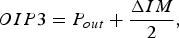
The output third order intercept point is given by
 $$OIP3 = P_{out} + \displaystyle{{\Delta IM} \over 2}\comma \;$$
where P out is the power level of the two fundamental tones and ΔIM is the difference in power level between the fundamental tone and the third order products.
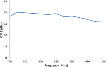
The OIP3 is shown in Fig. 15 as function of frequency.
OIP3 of NIC matched antenna.

The OIP3 is found to be similar to the OIP3 of other radio frequency (RF) front-end devices [Reference Marshall23] and is not expected to impact negatively on linearity of the overall system performance.
Using the cascade IP3 calculation in equation (16), it can be seen that the impact of the NIC matched antenna in a receiver mode is minimal as the IP3 of the overall system is dominated by the linearity of the later stage components. In transmit mode however, the IP3 performance will impact on the overall performance but this will not be significant as its IP3 value is within the range of other non-linear devices in the RF front-end.
 $$\displaystyle{1 \over {IIP3_{sys}^2 }} = \displaystyle{1 \over {IIP3_1^2 }} + \sum\nolimits_{i = 2}^n {\displaystyle{{G_1^2 G_2^2 G_3^2 \cdots \cdots G_{i - 1}^2 } \over {IIP3_i^2 }}}\comma \;$$
 $$IIP3 = OIP3 - Gain.$$
VI. CONCLUSION
This paper has demonstrated several important advances in the theory, design and implementation of NICs for the use in antenna matching. A customized stability analysis technique has been developed and applied to help show how to design a NIC for stable operation at high frequencies. The application of this method has been demonstrated in a practical NIC circuit working up to 1.5 GHz, the highest reported so far. The circuit fabrication technology available for this work made it impractical to integrate the prototype NIC with a practical antenna. However, important noise and non-linearity measurements have been carried out with the NIC connected to a passive circuit network designed to generate an impedance equivalent to that of the antenna over 700 MHz to 1 GHz, the widest practically achievable sample portion of the frequency range. By this method, it has been shown that NIC matching has a significant SNR advantage when compared to resistive passive matching, which is the only other practical way to achieve such a bandwidth enhancement. Similarly, as a measure of the non-linearity of the NIC, the third order intercept point has been shown to be comparable with other typical front end components using similar transistors.
The results demonstrate the potential for using NIC matching for electrically small or broadband antennas, up into the GHz frequency range. Further research is required for producing NIC elements in more suitable technology, such as MMIC, facilitating reduced size, direct integration, and further improved performance through reduced losses. MMIC technology would offer the further advantage of being able to select and scale transistor structures for an optimum combination of frequency range, stability, noise and linearity, for any given application.
 Oluwabunmi Tade received his B.Sc degree in Systems Engineering from the University of Lagos, Nigeria in 2005 and an M.Sc degree in Communications Engineering from the University of Birmingham, UK in 2009. He is a student member of EuMA. From 2007 to 2008, he was an NSS Engineer with Globacom Nigeria undertaking numerous network installations, upgrades, and integration. He is currently a Ph.D student with the Communications group of the School of Electronic, Electrical and Computer Engineering of the University of Birmingham. His research interests include: cognitive radio system and architecture, using non-Foster circuits to enhance performance of electrically small antennas for use in cognitive radio systems, and linearity measurement in active antennas.
 Peter Gardner has an MA in physics from the University of Oxford and a Ph.D in electronic engineering from the University of Manchester Institute of Science and Technology (UMIST). From 1981 to 1989, he was with Ferranti, Poynton, Cheshire, as Senior Engineer in microwave amplifiers, before joining the Department of EE&E at UMIST as a Research Associate working on microwave negative resistance circuits, low-noise MMIC design, and tunable resonators. In 1994, he joined the School of EECE at Birmingham University, where he is now Reader in Microwave Engineering. His current research interests include microwave and millimetric adaptive antennas and amplifier linearization.
 Peter Hall is Professor of Communications Engineering, leader of the Antennas and Applied Electromagnetics Laboratory, and Head of the Devices and Systems Research Centre in the Department of Electronic, Electrical and Computer Engineering at The University of Birmingham. After graduating with a Ph.D in antenna measurements from Sheffield University, he spent 3 years with Marconi Space and Defence Systems, Stanmore working largely on a European Communications satellite project. He then joined The Royal Military College of Science as a Senior Research Scientist, progressing to Reader in Electromagnetics. He joined The University of Birmingham in 1994. He has researched extensively in the areas of antennas, propagation, and antenna measurements. He has published five books, over 350 learned papers and taken various patents and awards. Professor Hall is a Fellow of the IEE and the IEEE and a past IEEE Distinguished Lecturer. He is a past Chairman of the IEE Antennas and Propagation Professional Group. He is a member of the IEEE AP-S Fellow Evaluation Committee. He is currently on the editorial board of Microwave and Optical Technology Letters. He received the LAPC IET James Roderick James Lifetime Achievement Award and in 2012 the EurAAP Award, and the IEEE AP-S John Kraus Award.