1. Introduction
While the primary justification for the creation of Social Security in 1935 was to create “more adequate provision for aged persons,”Footnote 1 today it accounts for 16–17% of total annual federal government expenditures, second only to health expenditures (excluding defense). Economists have traditionally viewed Social Security as a vehicle that partially insures individuals against risks that markets do not insure well, such as the risk of an uncertain lifetime, and the risk of unfavorable labor market outcomes causing old-age poverty. Social Security annuities are paid until death, so they are commonly believed to insure individuals against the risk of out-living their own savings. Meanwhile, Social Security benefits are a concave function of work-life earnings, and this concavity is intended to enable better work-retirement consumption smoothing, particularly when events such as unemployment and economic recessions negatively impact early life labor income.
While public pension programs, in general, are understood to have important insurance effects, there is also considerable evidence that such programs negatively affect households’ consumption, saving, and labor supply decisions. In particular, Social Security causes households to exit from the labor market earlier, to work fewer hours during employment, and to also reduce the personal savings needed for financing retirement consumption [Jeske (Reference Jeske2003), Wallenius (Reference Wallenius2013), Alonso-Ortiz (Reference Alonso-Ortiz2014)]. Therefore, the literature on Social Security’s overall welfare consequences has traditionally evolved as a comparison of the benefits of its insurance effects, to its distortionary costs on household behavior. This literature has broadly concluded that under traditional preferences, the welfare gains from the insurance effects of Social Security are usually smaller than its distortionary welfare losses [Auerbach and Kotlikoff (Reference Auerbach and Kotlikoff1987), Bagchi (Reference Bagchi2015)], although some find overall welfare gains, especially when labor supply is inelastic [Hubbard and Judd (Reference Hubbard and Judd1987), İmrohoroğlu et al. (Reference İmrohoroğlu, İmrohoroğlu and Joines1995)]. This literature, however, has typically ignored how Social Security m\right interact with a third type of risk: the risk related to one’s health status.
On the one hand, Social Security transfers resources from early life, when health risks are relatively low, to old age, when health risks are considerably higher. This transfer can potentially improve welfare, especially if households cannot save efficiently for uncertain old-age medical expenditures. While there are both public and private avenues that allow households to partially insure against health risks, such as Medicaid, Medicare, employment-based health insurance, and individual health insurance, the impact of Social Security on consumption smoothing in the context of health risk is not well understood. On the other hand, as households engage in precautionary savings due to the presence of health risk in their budget constraints, Social Security has a negative effect on disposable income in early life, especially for households that are borrowing constrained, which can distort precautionary savings and potentially reduce welfare. Traditional welfare analyses of Social Security have typically abstracted from health risks and have therefore overlooked these mechanisms [e.g., Hubbard and Judd (Reference Hubbard and Judd1987), İmrohoroğlu et al. (Reference İmrohoroğlu, İmrohoroğlu and Joines1995), Bagchi (Reference Bagchi2015)].
In this paper, we quantify the importance of idiosyncratic health risk in a calibrated general equilibrium model of Social Security. More specifically, we compare the welfare implications of Social Security in an environment with labor income, mortality, as well as health risks to those in an environment where health risk is removed from the model. To do this, we begin by constructing a calibrated general equilibrium macroeconomic model with households, firms, markets for goods and services, and a government that provides partial insurance against income and health risks. Then, we compute two common policy experiments with this model. First, in order to assess the overall welfare effects of Social Security in our model environment, we cut its payroll tax rate by 50% from its current level. Second, to evaluate how the degree of redistribution implicit in Social Security affects households with varying degrees of economic resources, we modify the progressivity of Social Security’s benefit-earnings rule. To tease out the precise effect of idiosyncratic health risk, we repeat these experiments in a hypothetical version of our model in which we completely remove idiosyncratic health risk from a household’s economic environment. More specifically, we still allow for exogenous health expenditure as an increasing function of age, but health expenditure does not vary by household type anymore and is therefore not a source of idiosyncratic risk but simply follows a deterministic trend that directly depends on age. We also examine the implications of these experiments for labor supply, consumption, and saving decisions, the markets for goods and services, the values of key macroeconomic aggregates, and the government’s budget.
In general, our findings indicate that idiosyncratic health risk has important implications for the welfare effects of Social Security. The presence of partially insured health risk, especially in old age, increases the long-term consumption smoothing benefits of Social Security, but its payroll tax reduces disposable income in early life and negatively affects short-term consumption smoothing by reducing a household’s ability to self-insure against such risk. We find that in our model framework, the short-term consumption smoothing effect dominates: downsizing Social Security always leads to higher overall welfare in general equilibrium, but the welfare gain is larger when we account for health risk. Similarly, we find that increasing the progressivity of Social Security’s benefit-earnings rule has a larger positive effect on overall welfare in the presence of health risk, and reduced progressivity has an almost identical negative effect both with and without health risk. In other words, our results from this experiment suggest that ignoring the effect of health risk on labor income, household expenditures, and survivorship in a general equilibrium environment underestimates the insurance value of Social Security.
Given that the key mechanism in our model is the trade-off between long- and short-term consumption smoothing, we examine how our computational results change when we allow households access to additional tools that help smooth health risk. We find that allowing for early Medicare eligibility (due to an event such as disability) weakens the precautionary motive, as a result of which downsizing Social Security leads to roughly identical welfare gains both with and without health risk. The same is true when we modify the progressivity of Social Security’s benefit-earnings rule: allowing for early Medicare, we find that the welfare gains from increased progressivity are roughly identical in models with and without health risk, and the welfare loss from reduced progressivity is significantly smaller in the presence of health risk.
The United States experienced a significant regulatory overhaul of its healthcare system more than a decade ago. On March 23, 2010, President Barack Obama signed into law the Patient Protection and Affordable Care Act, also known as the ACA, as the largest piece of healthcare reform legislation in the USA over the past 40 years. While there is a burgeoning literature that examines the implications of the ACA with respect to household-level healthcare spending and welfare, not much is known regarding the role of Social Security in providing insurance against health risks. Currently, economists and policymakers understand Social Security as providing insurance against income and mortality risks, and the literature has already shown that under traditional preferences, these effects may not be strong enough to yield overall welfare gains. However, insurance against health risks provides two separate channels through which Social Security m\right affect welfare:
 $\left (i\right)$
the self-insurance channel and
 $\left (ii\right)$
the redistribution of health risk channel. To the best of our knowledge, our paper is the first to quantitatively evaluate and compare the importance of these two channels.
The remainder of the paper is structured as follows. Section 2 briefly reviews the literature. Section 3 introduces the computational model. Section 4 outlines our baseline calibration. We discuss our computational experiments and their results in Section 5. Finally, we conclude in Section 6.
2. Related literature
As discussed in Glomm and Jung (Reference Glomm and Jung2013), government transfers can be classified as early (i.e., transfers to the young) vs. late (i.e., transfers to the old). Both transfers are associated with a certain level of tax distortions that the government can attempt to minimize. In this project, our objective is to examine the effects of health risk on the welfare implications of a late redistribution system—US Social Security—focusing either on the revenue or the spending side. We do this in an environment with realistic mortality, labor income, and health risks, where health risk affects household income, medical expenditures, and survivorship. This research contributes to several related strands of the literature.
First, starting with Abel (Reference Abel1985) and Hubbard and Judd (Reference Hubbard and Judd1987), a number of studies have examined the importance of the traditional roles of unfunded public pensions in justifying the size of US Social Security. Abel (Reference Abel1985) and Hubbard and Judd (Reference Hubbard and Judd1987) find a welfare-improving role for Social Security in a model with mortality risk and closed annuity markets, but Hubbard and Judd (Reference Hubbard and Judd1987) find that these welfare gains are significantly reduced or even eliminated when borrowing constraints are introduced. In a related study, İmrohoroğlu et al. (Reference İmrohoroğlu, İmrohoroğlu and Joines1995) examine the optimality of Social Security in a life cycle economy with mortality risk, missing annuity markets, idiosyncratic employment risk, and borrowing constraints. While this literature does not arrive at a consensus regarding the optimal size of Social Security in the USA, it generally concludes that the welfare-improving role of Social Security is much smaller once the consumption, saving, and labor supply distortions from Social Security are accounted for. Our analysis extends this literature by comprehensively accounting for health risk in a household’s budget constraint as well as the utility function, all within a calibrated general equilibrium model of Social Security.
Second, there are a number of studies that jointly examine Social Security and health risk in their model frameworks. For example, İmrohoroğlu and Kitao (Reference İmrohoroğlu and Kitao2012) evaluate Social Security reform proposals accounting for benefit claiming and labor force participation using a general equilibrium model with health risk, and Braun, et al. (Reference Braun, Kopecky and Koreshkova2017) evaluate the welfare implications of means tested social insurance, such as Medicaid and Supplemental Security Income, conditional on current US Social Security and health risk in a similar general equilibrium framework. Disability insurance (DI) and its connection to retirement have been studied in partial equilibrium frameworks by Low and Pistaferri (Reference Low and Pistaferri2015) and Blundell et al. (Reference Blundell, Britton, Dias and French2021).Footnote 2
More recently, Jones and Li (Reference Jones and Li2018; Reference Jones and Li2020) use a partial equilibrium framework and examine Social Security reform using models with health-dependent income, health expenditures, and mortality risk and conclude that the progressivity of US Social Security should be increased to a lump-sum benefit and the claiming adjustments should be reduced. Extending this literature, we use a general equilibrium model to specifically investigate the role of health risk on the insurance role of Social Security, as well as its effects on the degree of redistribution implicit in Social Security’s payout formula. We thereby quantify the marginal effect of health risk, that is, we examine how the welfare implications of Social Security change as we turn health risk on and off, which is a novel contribution to this literature.
Third, a rapidly growing macro-health literature has developed general equilibrium models with health to investigate either the sources of the increase in health spending [e.g., Suen (Reference Suen2006), Zhao (Reference Zhao2014)] or the effects of health insurance programs and their associated tax financing instruments [e.g., Jeske & Kitao (Reference Jeske and Kitao2009), Pashchenko and Porapakkarm (Reference Pashchenko and Porapakkarm2013), Jung and Tran (Reference Jung and Tran2016)]. However, because these studies mostly focus on either the sources of growth in medical spending or healthcare reform, they do not examine how Social Security’s insurance role interacts with health risk. In addition, they do not consider how Social Security’s implicit redistribution through the concave benefit-earnings rule affects the welfare of households with varying exposure to health risks. The current paper addresses these questions.
Finally, there is a large literature investigating optimal tax progressivity [e.g., Conesa and Krueger (Reference Conesa and Krueger2006), Heathcote et al. (Reference Heathcote, Storesletten and Violante2017), Jung and Tran (Reference Jung and Tran2022), Heer and Rohrbacher (Reference Heer and Rohrbacher2021)] and the effects of tax progressivity on tax revenue, wealth equality, and human capital accumulation [e.g., Holter et al. (Reference Holter, Krueger and Stepanchuk2019)]. While we do not focus on overall income tax progressivity, our experiments with the Social Security’s benefit-earnings rule are essentially examining the implications of modifying the degree of redistribution implicit in Social Security. Three recent papers that specifically look at the implications of modifying Social Security’s progressivity are Nishiyama and Smetters (Reference Nishiyama and Smetters2008), Golosov et al. (Reference Golosov, Shourideh, Troshkin and Tsyvinski2013), and Bagchi (Reference Bagchi2019). Nishiyama and Smetters (Reference Nishiyama and Smetters2008) show that the relatively long averaging period in Social Security’s benefit-earnings rule already provides substantial insurance against early life income uncertainty affecting retirement consumption, so the welfare gains from increased progressivity do not outweigh its distortions on labor supply and saving. Golosov et al. (Reference Golosov, Shourideh, Troshkin and Tsyvinski2013) use a model with deterministic earnings and a history-dependent benefit-earnings rule and show that more progressive benefit-earnings rules than the current US formula will improve welfare in a partial equilibrium setting. However, their analysis ignores factors such as idiosyncratic earnings and mortality risk, as well as health risk. On the other hand, Bagchi (Reference Bagchi2019) examines how the correlation between earnings and mortality risk interacts with the welfare effects of Social Security’s benefit-earnings rule, and finds that due to their lower expected utility from old-age consumption, poorer households with lower probability of survival do not necessarily benefit from increased progressivity. The key mechanisms that we capture in this paper that Nishiyama and Smetters (Reference Nishiyama and Smetters2008) and Bagchi (Reference Bagchi2019) ignore are the interactions of health risk with a household’s budget constraint, as well as their utility function. Our model features three channels through which health risk affects households: their labor income, their medical expenditures, and also their life expectancy. Arguably, accounting for all of these channels together within a calibrated general equilibrium environment leads us to new and different conclusions.
3. Model
We develop an overlapping generations model consisting of utility-maximizing households, profit-maximizing firms, and a government that provides consumption insurance for low-income households, Social Security, Medicare, and Medicaid.
3.1 Demographics
The economy is populated with overlapping generations of individuals who live a maximum of
 $J$
periods. Individuals are able to retire with benefits once they reach the eligible retirement age
 $J_{r}.$
This implies they are retired for at most
 $J-J_{r}+1$
periods. Since almost all households have fully retired at very high ages, we introduce a second age threshold
 $J_{R}$
after which retirement is enforced. This does not affect our results and helps reduce the computational burden.
In each period, individuals of age
 $j$
face an exogenous survival probability
 $\pi _{j}\!\left(\varepsilon ^{h}\right)$
that depends on their health state
 $\varepsilon ^{h}$
at age
 $j$
. In addition, the population grows exogenously at rate
 $\mathfrak{n}$
. We assume stable demographic patterns, so that age
 $j$
agents make up a constant fraction
 $\mu _{j}$
of the entire population at any point in time. The relative sizes of the cohorts alive
 $\mu _{j}$
and the mass of individuals dying
 $\tilde{\mu }_{j}$
in each period (conditional on survival up to the previous period) can be recursively defined as
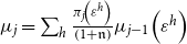 $\mu _{j}=\sum _{h}\frac{\pi _{j}\!\left(\varepsilon ^{h}\right)}{\left (1+\mathfrak{n}\right )}\mu _{j-1}\!\left(\varepsilon ^{h}\right)$
and
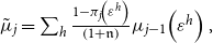 $\tilde{\mu }_{j}=\sum _{h}\frac{1-\pi _{j}\!\left(\varepsilon ^{h}\right)}{\left (1+\mathfrak{n}\right )}\mu _{j-1}\!\left(\varepsilon ^{h}\right),$
where
 $\mu _{j}\!\left(\varepsilon ^{h}\right)$
is the mass of individuals with health state
 $\varepsilon ^{h}$
. Accidental bequests
 $t^{\text{Beq }}$
are taxed by the government and redistributed to the surviving households as lump-sum transfers.
3.2 Preferences
The period utility function
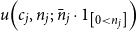 $u\!\left (c_{j},n_{j};\,\bar{n}_{j}\cdot 1_{\left [0\lt n_{j}\right ]}\right )$
depends on consumption
 $(c)$
, labor
 $(n)$
, and labor force participation status, captured by the indicator variable
 $1_{\left [0\leq n_{j}\right ]}$
, where
 $1_{\left [true\right ]}=1$
and
 $0$
otherwise. The age-dependent labor force participation cost (measured in hours) is given by
 $\bar{n}_{j}$
. When the individual dies, (s)he values bequests of assets
 $a_{j}$
according to the function
 $b\!\left (a_{j}\right ),$
which is increasing in asset holdings
 $a_{j}.$
3.3 Health status, health expenditure, and health insurance status
Health status
 $\varepsilon ^{h}$
is exogenous and evolves according to a Markov process with age and permanent income group-dependent transition probability matrix
 $\Pi _{j,\vartheta }^{h}$
. Transition probabilities to next period’s health status
 $\varepsilon _{j+1}^{h}$
depend not only on the current health status
 $\varepsilon _{j}^{h}$
but also on current age
 $j$
and the individuals permanent income group
 $\vartheta$
, so that an element of transition matrix
 $\Pi _{j,\vartheta }^{h}$
is defined as the conditional probability
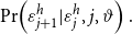 $\Pr \!\left (\varepsilon _{j+1}^{h}|\varepsilon _{j}^{h},j,\vartheta \right ).$
Health expenditures
 $m\!\left (\varepsilon _{j}^{h},j,\vartheta \right )$
at a certain age
 $j$
depend on the current health status
 $\varepsilon _{j}^{h}$
, age
 $j$
itself, and the permanent income group.
The health insurance state of a household at age
 $j$
,
 ${\text{HI}}_{j}\in \left \{ 0,1\right \},$
is determined when the household becomes economically active in the first model period and does not change thereafter. If the household has private employer provided insurance (EHI), then the indicator variable
 $\text{HI}_{j}=1$
, otherwise
 $\text{HI}_{j}=0$
. Once the household retires, the private health insurance state is
 $\text{HI}_{j}=0.$
We assume that a fixed percentage of every newborn cohort enters the model uninsured, that is, with
 $\text{HI}_{j}=0$
.
In addition, households qualify for Medicaid if they pass the Medicaid income and asset test. The indicator variable for Medicaid
 $1_{\left [\text{MAid-Yes}\right ]}$
equals one if adjusted gross income is less than the earnings threshold
 $y_{\text{AGI }}\lt y_{\text{MAid}}$
and the asset holdings are below the asset threshold
 $a\lt a_{\text{MAid}}$
and zero otherwise.
Finally, households also qualify for Medicare once they reach eligibility age
 $J_{r}$
. “Dual eligibles” are households that qualify for both, EHI and Medicaid before retirement or Medicare and Medicaid after retirement. In this case, Medicaid is the secondary insurance or the payer of last resort. For “Triple eligibles,” EHI is the primary insurance, Medicare is the secondary, and Medicaid is the tertiary insurance. The out-of-pocket medical expenditures are therefore insurance state dependent and can be written as
 \begin{align*} & o_{j}\!\left (m_{j},y_{\text{AGI},j},a_{j},\text{HI}_{j}\right ) \\[3pt] & \quad= \begin{cases} \left (1-\overset{\text{Primary HI}}{\overbrace{1_{\left [\text{MAid-Yes}\right ]}\kappa _{\text{MAid}}}}\right )\times m & \text{if\,}\ \overset{\text{working, no private HI}}{\overbrace{\text{HI}=0\,\wedge \,j\lt J_{r}}}\\ \\ \left (\left (1-\overset{\text{Primary}}{\overbrace{\kappa _{\text{EHI}}}}\right )-\overset{\text{Medicaid is secondary HI}}{\overbrace{1_{\left [\text{MAid-Yes}\right ]}\kappa _{\text{MAid}}\!\left (1-\kappa _{\text{EHI}}\right )}}\right )\times m & \text{if}\,\ \overset{\text{working, with private HI}}{\overbrace{\text{HI}_{j}=1\,\wedge \,{j\lt J_{r}}}}\\ \\ \left (\begin{array}{c} \left (\left (1-\overset{\text{Primary}}{\overbrace{\kappa _{\text{EHI}}}}\right )-\overset{\text{Medicare is secondary HI}}{\overbrace{\kappa _{\text{MCare}}\!\left (1-\kappa _{\text{EHI}}\right )}}\right )\\ \\ -\overset{\text{Medicaid is tertiary HI}}{\overbrace{1_{\left [\text{MAid-Yes}\right ]}\kappa _{\text{MAid}}\!\left (\left (1-\kappa _{\text{EHI}}\right )-\kappa _{\text{MCare}}\!\left (1-\kappa _{\text{EHI}}\right )\right )}} \end{array}\right )\times m & \text{if}\,\ \overset{\text{Medicare, working with private HI}}{\overbrace{\text{HI}_{j}=1\,\wedge \,j \geq J_{r}\,\wedge \,n_{j}\gt 0}},\\ \\ \left (\left (1-\overset{\text{Primary}}{\overbrace{\kappa _{\text{MCare}}}}\right )-\overset{\text{Medicaid is secondary HI}}{\overbrace{1_{\left [\text{MAid-Yes}\right ]}\kappa _{\text{MAid}}\!\left (1-\kappa _{\text{MCare}}\right )}}\right )\times m & \text{if}\,\overset{\text{Medicare eligible, no private HI, working or retired}}{\overbrace{\text{HI}_{j}=0\,\wedge \,j\geq J_{r}\,\wedge \,n_{j}\geq 0}}, \end{cases} \end{align*}
where
 $\kappa _{\text{EHI}}$
is the reimbursement rate of EHI,
 $\kappa _{\text{MAid}}$
is the reimbursement rate of Medicaid, and
 $\kappa _{\text{MCare}}$
is the reimbursement rate of Medicare. Households with EHI pay a premium of
 $p_{\text{EHI}}$
every period, and households on Medicare pay Medicare Plan B Premium of
 $p_{\text{MCare}}$
.
3.4 Income process
Conditional on labor force participation, a household earns before-tax wage income
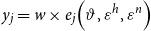 $y_{j}=w\times e_{j}\!\left(\vartheta,\varepsilon ^{h},\varepsilon ^{n}\right)$
 $\times n_{j}$
at age
 $j$
, where
 $w$
is the wage rate, and
 $e_{j}\!\left(\vartheta,\varepsilon ^{h},\varepsilon ^{n}\right)$
is a labor productivity endowment that depends on age
 $j$
, a permanent income group
 $\vartheta$
, an idiosyncratic productivity shock
 $\varepsilon ^{n}$
, and most notably, health status
 $\varepsilon ^{h}$
. The transition probabilities for the idiosyncratic productivity shock
 $\varepsilon ^{n}$
follow a Markov process with transition probability matrix
 $\Pi ^{n}.$
Let an element of this transition matrix be defined as the conditional probability
 $\Pr \!\left (\varepsilon _{j+1}^{n}|\varepsilon _{j}^{n}\right )$
, where the probability of next period’s labor productivity
 $\varepsilon _{j+1}^{n}$
depends on today’s productivity
 $\varepsilon _{j}^{n}.$
3.5 Technology and factor prices
The economy consists of firms that use physical capital
 $K$
and effective labor services
 $N$
to produce output. Firms are perfectly competitive and solve the following maximization problem:
 \begin{equation} \max _{\left \{ K,\,N\right \} }\!\left \{ F\!\left (K,N\right )-q\times K-w\times N\right \}, \end{equation}
taking the rental rate of capital
 $q$
and the wage rate
 $w$
as given. Capital depreciates at rate
 $\delta$
in each period.
3.6 Government
The government collects five separate taxes: a consumption tax at rate
 $\tau _{C}$
, a tax on accidental bequests at rate
 $\tau _{B}$
, a progressive income tax on taxable income
 $y_{j}$
denoted
 $T_{y}(y_{j})$
, and payroll taxes
 $T_{ss}\!\left(y_{j}^{n};\,\bar{y}\right)$
and
 $T_{\text{MCare}}\!\left(y_{j}^{n}\right)$
for Social Security and Medicare, respectively, collected on labor income
 $y_{j}^{n}$
. The payroll tax for Social Security is proportional only up to the maximum taxable earnings of
 $\bar{y}$
. With these tax revenues, the government runs the following spending programs: Social Security, Medicare, Medicaid, lump-sum transfers to low-income earners to guarantee a minimum consumption level
 $\underline{c}$
, and general public goods purchases.
Households receive Social Security benefits after the eligibility age
 $\left (J_{r}\right )$
if they do not participate in the labor market (i.e., if
 $n_{j}=0$
), and the amount of benefits paid to a particular household depends on its earnings history. For each household, the government calculates an average of past earnings (up to the maximum taxable earnings), referred to as the average indexed monthly earnings
 $(\text{AIME})$
. The Social Security benefit amount, also called the primary insurance amount (PIA),
 $b_{ss,j}\!\left (\text{AIME}\right )$
is a function of AIME.
Households become eligible for Medicare after age
 $J_{r},$
at which point they also start paying a Medicare premium
 $p_{\text{MCare}}$
every period. We assume that the government’s budgets, both for Social Security and Medicare, are balanced.Footnote
3
This implies
 \begin{gather} \int 1_{\left [j\geq J_{r}\right ]}b_{ss}\!\left (\text{AIME}\!\left (\boldsymbol{x}\right )\right )d\Lambda (\boldsymbol{x})=\int T_{ss}\!\left (w\times e(\boldsymbol{x})\times n(\boldsymbol{x});\,\bar{y}\right )\!d\Lambda (\boldsymbol{x}), \end{gather}
and
 \begin{equation} \int 1_{\left [j\geq J_{r}\right ]}\kappa _{\text{MCare}}\times m(\boldsymbol{x})d\Lambda (\boldsymbol{x})=\int \!\left (T_{\text{MCare}}\!\left (w\times e(\boldsymbol{x})\times n(\boldsymbol{x})\right )+1_{\left [j\geq J_{r}\right ]}p_{\text{MCare}}\right )\!d\Lambda (\boldsymbol{x}). \end{equation}
Households are also eligible for Medicaid payments if they pass the income and asset tests
 $y(\boldsymbol{x})\lt y_{\text{MAid}}$
and
 $a_{j}\lt a_{\text{MAid}}$
, respectively. The government also finances a minimum consumption floor
 $c_{min}$
with social transfers
 $b_{si}.$
The expenditures on public goods purchases
 $G$
are the residual such that its total revenues from capital and labor income taxes are sufficient to finance its total spending:
 \begin{align} & G+\overset{\text{Medicaid payments}}{\overbrace{\int \!\left (1_{\left [\text{MAid-Yes}\right ]}\kappa _{\text{MAid}}\times m(\boldsymbol{x})\right )d\Lambda (\boldsymbol{x})}}+\overset{\text{social transfers}}{\overbrace{\int b_{si}\!\left (\boldsymbol{x}\right )d\Lambda (\boldsymbol{x})}}=\int T_{y}\!\left (y(\boldsymbol{x})\right )d\Lambda (\boldsymbol{x})onumber\\[4pt]& \quad +\tau _{C}\int c(\boldsymbol{x})d\Lambda (\boldsymbol{x})+\tau _{B}\int t^{\text{Beq}}(\boldsymbol{x})d\Lambda (\boldsymbol{x}). \end{align}
3.7 Insurance companies
Private insurance companies maximize profits with free entry so that premiums
 $p_{\text{EHI}}$
clear the following zero-profit condition
 \begin{gather} \kappa _{\text{EHI}}\int 1_{\left [\text{HI}_{j}=1\,\land \,\text{MAid-No}\right ]}m(\boldsymbol{x})d\Lambda (\boldsymbol{x})=p_{\text{EHI}}\int 1_{\left [\text{HI}_{j}=1\,\land \,y_{j}(x)\gt y_{\text{MAid}}\right ]}d\Lambda (\boldsymbol{x}). \end{gather}
3.8 The household maximization problem
The state vector of a household at a particular age is defined as
 $x_{j}=\left \{ \vartheta,a_{j},\text{AIME}_{j},\text{HI}_{j},\varepsilon _{j}^{n},\varepsilon _{j}^{h}\right \} \in \left \{ 1,2,3\right \} \times R^{+}\times R^{+}\times \left \{ 0,1\right \} \times \times \left \{ 1,2,3,4,5\right \} \times \left \{ 1,2,3,4,5\right \}$
, where
 $\vartheta$
denotes the permanent income group of no-school, high-school, and college types,
 $a_{j}$
denotes the beginning-of-period assets,
 $\text{AIME}_{j}$
denotes the average past earnings that determine Social Security benefits,
 $\text{HI}_{j}$
denotes the deterministic health insurance state,
 $\varepsilon _{j}^{n}$
denotes the labor shock, and
 $\varepsilon _{j}^{h}$
denotes the health state.
After the realization of the state variables, agents simultaneously chose from their choice set
 \begin{equation*} \mathcal {C}_{j}\equiv \left \{ \left (c_{j},n_{j},a_{j+1}\right )\in R_{+}\times \left [0,1\right ]\times R_{+}\right \} \end{equation*}
where
 $c_{j}$
is the consumption,
 $n_{j}$
is the labor, and
 $a_{j+1}$
are asset holdings for the next period, in order to maximize their lifetime utility. All choice variables in the optimization problem are functions of the state vector but we suppress this notation in order to not clutter the exposition.
3.8.1 Working households
The household problem of the working household can be recursively written as
 \begin{align} V\!\left (x_{j}\right ) & =\max _{\left \{ c_{j},n_{j},a_{j+1}\right \} }\left \{ u\!\left (c_{j},n_{j};\,\bar{n}_{j}\cdot 1_{\left [0\lt n_{j}\right ]}\right )+\beta \!\left (\pi _{j}\!\left (\varepsilon{}^{h}\right )\times \mathbb{E}\left [V\!\left (x_{j+1}\right )|\,x_{j}\right ] \left (1-\pi _{j}\!\left (\varepsilon{}^{h}\right )\right )b\!\left (a_{j+1}\right )\right )\right \} onumber\\ & s.t. \end{align}
 \begin{align} \left (1+\tau _{C}\right )c_{j}& + a_{j+1}\overset{\text{Out-of-pocket medical spending}}{\overbrace{+o_{j}\!\left (m_{j},y_{\text{AGI},j},a_{j},\text{HI}_{j}\right )+}}1_{\left [\text{HI}_{j}=1\,\land \,\text{MAid-No}\right ]}p_{\text{EHI}}+1_{\left [j\geq J_{r}\right ]}p_{\text{MCare}}+T_{y}\!\left (y_{j}\right )onumber\\& +T_{\text{ss}}\!\left (y_{n,j};\,\bar{y}\right )+T_{\text{MCare}}\!\left (y_{n,j}\right )onumber\\& =\left (1+r\right )a_{j}+y_{n,j}+1_{\left [j\geq J_{r},n_{j}=0\right ]}b_{ss,j}\!\left (\text{AIME}{}_{j}\right )+b_{si,j}+\left (1-\tau _{B}\right )t^{\text{Beq}}, c_{j}\geq \underline{c},\,a_{j}\geq 0, \end{align}
where
 $\beta$
is a time preference factor,
 $\pi _{j}\!\left (h_{j}\right )$
is the age and health state-dependent survival probability,
 $w$
is the market wage rate,
 $r$
is the interest rate, and
 $o_{j}$
is out-of-pocket medical spending as a function medical spending, income, asset holding, and private health insurance state. EHI premiums
 $p_{\text{EHI}}$
are only paid if the individual has private insurance from the employer so that
 $\text{HI}_{j}=1$
and the individual does not qualify for Medicaid (i.e., MAid-No). The Medicare Plan B premium is denoted
 $p_{\text{MCare}}$
and the after tax income is defined as
 \begin{equation} y_{j}^{\text{at}}=y_{\text{AGI,}j}-T_{y}\!\left (y_{j}\right )-T_{\text{ss}}\!\left (y_{n,j};\,\bar{y}\right )-T_{\text{MCare}}\!\left (y_{n,j}\right ), \end{equation}
where
 $\tau _{C}$
is a consumption tax,
 $T_{y}$
is the progressive income tax, which is a function of taxable household income
 $y_{j}$
,
 $T_{\text{ss}}$
is Social Security’s payroll tax, also a function of labor income
 $y_{n,j}$
(up to a taxable maximum
 $\bar{y}),$
 $T_{\text{MCare}}$
is Medicare’s payroll tax, and
 $\tau _{B}$
is a tax on accidental bequests
 $t^{\text{Beq}}$
. Labor income
 $y_{n,j}$
and total taxable income
 $y_{j}$
are defined as
 \begin{align} y_{n,j} & =w\overset{\text{Health-dependent labor income}}{\overbrace{\times e_{j}\!\left(\vartheta,\varepsilon ^{h},\varepsilon ^{n}\right)\times }}n_{j},onumber\\ y_{\text{AGI},j} & =y_{n,j}+r\times a_{j}+1_{\left [j\geq J_{r}\right ]}b_{ss,j}\!\left (\text{AIME}{}_{j}\right ),onumber \\ y_{j} & =y_{\text{AGI},j}-1_{\left [\text{HI}_{j}=1\,\land \,\text{MAid-No}\right ]}p_{\text{EHI}}onumber\\&\quad -\max \left [0,\left (o_{j}\!\left (m_{j},y_{\text{AGI},j},a_{j},\text{HI}_{j}\right )+1_{\left [j\geq J_{r}\right ]}p_{\text{MCare}}\right )-0.075\times y_{\text{AGI},j}\right ], \end{align}
where
 $y_{\text{AGI},j}$
is adjusted gross income. In addition, private health insurance premiums are tax deductible as are out-of-pocket health expenses and Medicare premiums that exceed
 $7.5$
% of
 $y_{\text{AGI}}$
.Footnote
4
Social Security payments are denoted
 $b_{ss,j}$
and social transfers are defined as
 \begin{align*} b_{si,j} & =\max \left [0,\text { }\left (1+\tau _{C}\right )\underline {c}+o_{j}\!\left (m_{j}\right )+1_{\left [\text {HI}_{j}=1\,\land \,\text {MAid-No}\right ]}p_{\text {EHI}}\right.\\& \quad +\left. 1_{\left [j\geq J_{r}\right ]}p_{\text {MCare}}-y_{j}^{\text {at}}-a_{j}-\left (1-\tau _{B}\right )t^{\text {Beq}}\right ], \end{align*}
and ensure a minimum consumption floor
 $\underline{c}$
after medical expenses, insurance premiums, and taxes are paid for. A household consuming at the lower bound cannot save into the next period.
Average past labor earnings follow:
 \begin{equation*} \text {AIME}{}_{j+1}=\begin {cases} \min \left (\frac {\left (j-1\right )\times \text {AIME}_{j}+y_{n,j}}{j},\bar {y}\right ) & \text {if}\ 1\leq j\lt J_{r},\\[4pt] \text {AIME}_{j} & \text {if}\ j\geq J_{r}, \end {cases} \end{equation*}
and
 \begin{align*} 0 & \leq n_{j}\leq 1, \end{align*}
and
 $J_{r}$
is the eligibility age for Social Security and Medicare. The indicator functions are defined as
 $1_{\left [true\right ]}=1$
and
 $1_{\left [false\right ]}=0$
.
3.8.2 Retired households
Households can stop working at any time; however, they receive Social Security benefits and qualify for Medicare starting at or after age
 $j\geq J_{r}$
and are forced to retire at age
 $j\geq J_{R}$
, where
 $J_{r}\lt J_{R}$
.Footnote
5
A retired households optimization problem reduces to
 \begin{align} V\!\left (x_{j}\right ) & =\max _{\left \{ c_{j},a_{j+1}\right \} }\left \{ u\!\left (c_{j}\right )+\beta \!\left (\pi _{j}\!\left (\varepsilon{}^{h}\right )\mathbb{E}\left [V\!\left (x_{j+1}\right )|\,x_{j}\right ]+\left (1-\pi _{j}\!\left (\varepsilon{}^{h}\right )\right )b\!\left (a_{j+1}\right )\right )\right \}onumber \\ & s.t. \end{align}
 \begin{align*} \left (1+\tau _{C}\right )c_{j}+a_{j+1}+o_{j}\!\left (m_{j}\right )+p_{\text{MCare}}+T_{y}\!\left (y_{j}\right )& =\left (1+r\right )a_{j}+b_{ss,j}\!\left (\text{AIME}{}_{j}\right )+b_{si,j}+\left (1-\tau _{B}\right )t^{\text{Beq}},\\& c_{j}\geq \underline{c},\,a_{j}\geq 0, \end{align*}
where after tax income is
 \begin{equation} y_{j}^{\text{at}}=y_{\text{AGI,}j}-T_{y}\!\left (y_{j}\right ), \end{equation}
and adjusted gross income
 $y_{\text{AGI }}$
and taxable income
 $y_{j}$
(net of bequests) are defined as
 \begin{align*} y_{\text{AGI},j} & =r\times a_{j}+b_{ss,j}\!\left (\text{AIME}{}_{j}\right ).\\ y_{j} & =y_{\text{AGI},j}-\max \left [0,\left (o_{j}\!\left (m_{j}\right )+1_{\left [j\geq J_{r}\right ]}p_{\text{MCare}}\right )-0.075\times y_{\text{AGI},j}\right ]. \end{align*}
We assume that all retired households are on Medicare so that out-of-pocket spending is only a function of medical spending. Social transfers are expressed as
 \begin{equation*} b_{si,j}=\max \left [0,\text { }\left (1+\tau _{C}\right )\underline {c}+o_{j}\!\left (m_{j}\right )+p_{\text {MCare}}-y_{j}^{\text {at}}-a_{j}-\left (1-\tau _{B}\right )t^{\text {Beq}}\right ]. \end{equation*}
3.8.3 Aggregation
We denote
 $\boldsymbol{x}\equiv \left \{ j,\,x_{j}\right \}$
as the augmented state vector including age
 $j$
and
 $\Lambda \!\left (\boldsymbol{x}\right )$
is the measure of households with state
 $\boldsymbol{x}$
which incorporates the relative cohort sizes
 $\mu _{j}$
.
3.9 Equilibrium
Given the transition probability matrices
 $\left \{ \Pi _{j}^{h},\Pi _{j}^{n}\right \} _{j=1}^{J},$
the survival probabilities
 $\left \{ \pi _{j}\!\left(\varepsilon ^{h}\right)\right \} _{j=1}^{J}$
, and the exogenous government policies
 $\left \{ \tau _{C},\tau _{B},T_{y},T_{\text{ss}},T_{\text{MCare}},b_{si},b_{ss},\kappa _{\text{MCare}},\kappa _{\text{MAid}},G\right \} _{j=1}^{J},$
a stationary competitive equilibrium is a collection of sequences of distributions
 $\Lambda \!\left (\boldsymbol{x}\right )$
of individual household decisions
 $\left \{ c\!\left (\boldsymbol{x}\right ),n\!\left (\boldsymbol{x}\right ),a\!\left (\boldsymbol{x}\right )\right \},$
aggregate stocks of physical capital and effective labor services
 $\left \{ K,L\right \},$
factor prices
 $\left \{ w,q,R\right \},$
and insurance premiums
 $\text{prem}^{\text{GHI}}$
such that:
 $\left (a\right )$
 $\left \{ c\!\left (\boldsymbol{x}\right ),n\!\left (\boldsymbol{x}\right ),a\!\left (\boldsymbol{x}\right )\right \}$
solves the consumer problem (6,7),
 $\left (b\right )$
the firm first-order conditions hold in both sectors
 \begin{eqnarray*} w & = & \frac{\partial F\!\left (K,L\right )}{\partial L},\\ q & = & \frac{\partial F\!\left (K,L\right )}{\partial K},\\ R & = & 1+q-\delta =1+r, \end{eqnarray*}
 $\left (c\right )$
markets clear
 \begin{align} K=\int a(\boldsymbol{x})d\Lambda (\boldsymbol{x}) \end{align}
 \begin{align} L=\int e(\boldsymbol{x})n(\boldsymbol{x})d\Lambda (\boldsymbol{x}). \end{align}
 \begin{eqnarray*} T^{\text{Beq}} & = & \sum \limits _{j=1}^{J}\tilde{\mu }_{j}\int a_{j}\!\left (x_{j}\right )d\Lambda \!\left (x_{j}\right ), \end{eqnarray*}
 $\left (d\right )$
the aggregate resource constraint holds
 \begin{equation*} G+K'+\int \!\left (c\!\left (\boldsymbol{x}\right )+m\!\left (\boldsymbol{x}\right )\right )d\Lambda \!\left (\boldsymbol{x}\right )=Y+\left (1-\delta \right )K, \end{equation*}
 $\left (e\right )$
the government programs clear so that (2), (3), and (4) hold,
 $\left (f\right )$
the budget conditions of the insurance companies (5) hold, and
 $\left (g\right )$
the distribution is stationary
 \begin{equation*} \left (\mu _{j+1},\Lambda\! \left (x_{j+1}\right )\right )=T_{\mu,\Lambda }\!\left (\mu _{j},\Lambda \!\left (x_{j}\right )\right ), \end{equation*}
where
 $T_{\mu,\Lambda }$
is a one period transition operator on the measure distribution
 \begin{equation*} \Lambda \!\left (\boldsymbol{x}^{\prime}\right )=T_{\Lambda }\!\left (\Lambda \!\left (\boldsymbol{x}\right )\right ). \end{equation*}
4. Calibration
We calibrate the model developed in the previous section to match the US economy. We entertain macroeconomic data targets such as overall capital accumulation, pattern of labor supply and health/medical expenditures over the life cycle, the life cycle pattern of income heterogeneity, and also the share of medical and government expenditures in GDP. While calibrating the model, we pay special attention to the payout formula of Social Security and some of the features of the Medicare and Medicaid programs.Footnote 6
For the calibration, we distinguish between two sets of parameters:
 $\left (i\right )$
externally selected parameters and
 $\left (ii\right )$
internally calibrated parameters. Externally selected parameters are estimated independently from our model and are either based on our own estimates using data from the Medical Expenditure Panel Survey (MEPS) or the Panel Survey of Income Dynamics (PSID) for the 1999–2009 period or estimates provided by other studies. We summarize these external parameters in Table 1. Internally calibrated parameters are assigned values so that model-generated data match a given set of targets from US data. Model-generated data moments and target moments from US data are juxtaposed in Table 2. In addition, we contrast model-generated moments that were not targeted by our calibration with moments from the data in Table 3 to demonstrate the performance of the model.
External parameters

Notes: These parameters are based on our own estimates from MEPS and CMS data as well as other studies.
Calibrated (endogenous) parameters

Notes: We choose these parameters in order to match a set of target moments in the data. We choose internal parameters so that model-generated data match data from MEPS, CMS, and NIPA.
*We do not distinguish between Medicare and Medicaid for the population older than 65. We therefore compare the size of Medicare in the model to the spending of Medicare plus Medicaid on individuals older than 65 to capture the out-of-pocket spending of the older generation more realistically without explicitly modeling Medicaid past the age of 65. According to NHEA (2020b ), aggregate Medicare spending in 2010 was approximately 3.47% of GDP. More details are provided in Section 4.
Model performance

Notes: These are not calibration targets.
Data source is MEPS 1999–2009, heads of HIEU, population we\righted, PSID 1999–2009 heads of households, population we\righted and SSA (2010).
**Medicaid in the model refers to the portion of Medicaid that targets the working age population. According to NHEA (2020b ), aggregate Medicaid payments for individuals younger than 65 in 2010 were approximately 1.7% of GDP. More details are provided in Section 4.
4.1 Demographics
One model period is defined as 1 year. We model households from age
 $25$
to age
 $99$
which results in
 $J=75$
periods. The labor supply choice periods are
 $j\in [0,\,J_{R}]=[0,60]$
which corresponds to ages
 $25$
and
 $84$
, respectively. Once the individual enters period
 $61$
, that is, age
 $85$
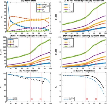
, (s)he is forced to exit the labor force. Panel [6] in Figure 1 depicts health state-dependent survival probabilities, which we obtain from estimates in İmrohoroğlu and Kitao (Reference İmrohoroğlu and Kitao2012). In the model, we distinguish between healthy and sick individuals which we discuss in greater detail in Section 4.3 below. Given these survival probabilities and the number of healthy vs. sick individuals generated by the model’s exogenous health process, we adjust the population growth rate
 $\mathfrak{n}$
to match the fraction of individuals older than
 $65$
.
Exogenous health state process and health spending shocks. Notes: Healthy is defined as the head of the HIEU reporting either excellent, very good, or good health. Sick is defined as fair or poor health. Data source is MEPS 1999–2009, heads of HIEU, population we\righted. All dollar values are denominated in 2009 dollars using the OECD CPI for the USA. The survival probabilities in panel [5] are from İmrohoroğlu and Kitao (Reference İmrohoroğlu and Kitao2012) who base their estimates on data from the Health and Retirement Study and life table estimates in Bell and Miller (Reference Bell and Miller2005).

4.2 Preferences
We specify period utility as
 \begin{equation*} u\!\left (c_{j},l_{j};\,\bar {n}_{j}\right )=\frac {\left (c_{j}^{\eta }\times \left [1-n_{j}-\bar {n}_{j}\cdot 1_{\left [0\lt n_{j}\right ]}\right ]{}^{1-\eta }\right )^{1-\sigma }}{1-\sigma }. \end{equation*}
We set the relative risk aversion parameter
 $\sigma$
to
 $3$
, and the intertemporal discount factor
 $\beta$
to
 $0.998$
to match the capital-output ratio target in equilibrium. Labor is chosen from a grid
 $n\in \left \{ 0,n_{\min },\ldots,n_{\max }\right \}$
where the minimum amount of non-zero labor possible is
 $n_{\min }=300$
hours per year, set to match the fraction of retirees at age 65, and the maximum amount of labor possible is set to
 $n_{\max }=80$
work hours per week. The fixed cost of working
 $\bar{n}_{j}$
is set to match the labor participation rate by age group from MEPS. The consumption intensity parameter
 $\eta$
is
 $0.4$
to match average labor hours of the working population. The warm glow bequest function is
 \begin{equation*} b\!\left (a_{j}\right )=\theta _{0}\frac {\left (a_{j}+\theta _{1}\right )^{\left (1-\sigma \right )\eta }}{1-\sigma }, \end{equation*}
where
 $\theta _{1}$
determines the curvature of the function.Footnote
7
We set
 $\theta _{1}=\$500,000$
as in De Nardi (Reference De Nardi2004) and French (Reference French2005) and scale parameter
 $\theta _{0}$
to match the average asset holdings of 90-year olds.
4.3 Health status, health expenditure, and health insurance status
We use data from MEPS 1999–2009 to estimate the magnitude of the age-dependent health expenditure shocks
 $m\!\left (\varepsilon _{j}^{h},j,\vartheta \right )$
as well as the Markov transition probability matrix
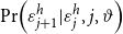 $\Pr \!\left (\varepsilon _{j+1}^{h}|\varepsilon _{j}^{h},j,\vartheta \right )$
which depends on age
 $j$
and the permanent income group
 $\vartheta$
. We group individuals into five health groups so that
 $\varepsilon ^{h}$
 $\in \left \{ 1,2,3,4,5\right \}$
by self-reported health status: 1. excellent health, 2. very good health, 3. good health, 4. fair health, and 5. poor health. We then calculate average medical spending of each health group by age and permanent income group to determine the magnitude of the health spending shocks
 $m\!\left (\varepsilon _{j}^{h},j,\vartheta \right )$
. Since MEPS only accounts for about 65–70% of healthcare spending in the national accounts [see Sing et al. (Reference Sing, Jessica, Selden, Cowan and Keehan2006); Bernard et al. (Reference Bernard, Cowan, Selden, Cai, Catling and Heffler2012)] we scale up the medical spending profiles for individuals older than 65 similar to Pashchenko and Porapakkarm (Reference Pashchenko and Porapakkarm2013).
We next estimate an ordered logit model to determine the conditional probability of moving to a specific health group
 $\varepsilon _{j+1}^{h}$
in year
 $t+1$
conditional on being a member of health group
 $\varepsilon _{j}^{h}$
at time
 $t$
of a
 $j$
year old individual using a fourth-order age polynomial. We control for permanent income groups
 $\vartheta$
which allows for education-specific health shock processes over age.
Following Zhao (Reference Zhao2014), we assume that the fraction of newborn households with employer provided health insurance,
 $\text{HI}_{j}=1$
is
 $75$
%. At the age of 65, households become eligible for Medicare and are assumed to enroll in it. A household is eligible for Medicaid if it passes an earnings and an assets test, which can become their secondary insurance if they already have private insurance or Medicare. In rare cases, Medicaid may be tertiary insurance if households that are older than 65 are still working and qualify for Medicare. In this case, Medicare becomes primary insurance, private employer-sponsored insurance is secondary, and Medicaid functions as tertiary insurance.
4.4 Income process
To calibrate the labor income process, we assume that labor productivity at age
 $j$
can be decomposed as
 \begin{equation} e_{j}\!\left(\vartheta,\varepsilon ^{h},\varepsilon ^{n}\right)=\bar{e}_{j}\!\left (\vartheta,h\!\left(\varepsilon ^{h}\right)\right )\times \varepsilon ^{n}, \end{equation}
where
 $\bar{e}_{j}$
 $\left (\vartheta,h\right )$
is deterministic in age
 $j$
, education level
 $\vartheta$
, and health state
 $h$
, and
 $\varepsilon ^{n}$
is a stochastic component that follows an auto-regressive process
 \begin{gather} \ln \left (\varepsilon _{j}^{n}\right )=ho \times \ln \left (\varepsilon _{j-1}^{n}\right )+\epsilon _{j}, \end{gather}
with persistence parameter
 $ho$
and a white-noise disturbance
 $\epsilon _{j}\sim N\!\left (0,\sigma _{\epsilon }^{2}\right )$
.
The
 $h\!\left(\varepsilon ^{h}\right)$
health state is binary and defined as
 \begin{equation*} h\!\left(\varepsilon ^{h}\right)=\begin {cases} \text {healthy} & \text {if}\ {\varepsilon }^{h}\in \left \{ 1,2,3\right \} \\ \text {sick} & \text {if}\ {\varepsilon }^{h}\in \left \{ 4,5\right \}. \end {cases} \end{equation*}
These are standard definitions for healthy/sick in the macro-health literature. The education level is permanent and fixed at age 20. We define three permanent educational groups:
 \begin{equation*} \vartheta =\begin {cases} 1 & \text {if less than high school},\\ 2 & \text {if high school},\\ 3 & \text {if college graduate or higher.} \end {cases} \end{equation*}
Figure 1 depicts the fraction of healthy individuals per age group and Table D.1 shows the relative cohort sizes of healthy/sick types by permanent income group.
4.4.1 Stochastic component
To calibrate the stochastic component
 $\varepsilon ^{n}$
, we use
 $ho =0.977$
and
 $\sigma _{\epsilon }^{2}=0.0141$
based on estimates from French (Reference French2005) who uses PSID data and controls for cohort effects and health states. We approximate the joint distribution of the persistent and transitory shocks using a five-state first-order discrete Markov process following Tauchen and Hussey (Reference Tauchen and Hussey1991).
4.4.2 Deterministic component
Using 1999–2009 MEPS data, we construct cohort-adjusted and bias-corrected wage profiles for each subgroup
 $\left (\vartheta,h\right )$
. Table D.1 shows the relative cohort sizes of these types in the population. We use observations from the head of health insurance eligibility units (HIEU) and limit the sample by focusing on individuals with labor incomes larger than
 $\$400$
.Footnote
8
We then use hourly wage observations of the head of a HIEU, deflate this variable with the urban Consumer Price Index (CPI), and remove cohort effects. We then follow the procedure in Rupert and Zanella (Reference Rupert and Zanella2015) and Casanova (Reference Casanova2013) and estimate a selection model to remove the selection bias that is typically associated with wage observations to get an average wage offer rate for each
 $\left (\vartheta,h\right )$
subgroup. We finally smooth the wage profiles with a second-degree polynomial in age.
4.5 Technology and factor prices
We assume that output is produced using a Cobb-Douglas production function with inputs capital and labor
 \begin{equation} Y=A\times K^{\alpha }\times N{}^{(1-\alpha )}, \end{equation}
where
 $\alpha$
is the share of capital in total income. We set the capital share to
 $\alpha =0.35$
and the annual capital depreciation rate to
 $\delta =0.064$
and normalize the total factor productivity
 $A$
to unity.
4.6 Government
4.6.1 Taxes
The consumption tax rate,
 $\tau _{C}$
, is set to
 $5$
%. The tax on bequests
 $\tau _{B}$
is set to 100%, similar to Conesa and Krueger (Reference Conesa and Krueger2006). This means that all accidental bequests are collected by the government. The income tax function is progressive and has the following specification:
 \begin{equation*} T_{y}(y)=\max \left [0,\,y-\tau _{0}\times y^{\left (1-\tau _{1}\right )}\right ], \end{equation*}
where
 $T_{y}(y)$
denotes net tax revenues as a function of pre-tax income
 $y$
,
 $\tau _{1}$
is the progressivity parameter, and
 $\tau _{0}$
is a scaling factor to match US income tax revenue.Footnote
9
We impose a non-negative tax payment restriction in the benchmark model,
 $T_{y}(y)\geq 0$
. This restriction excludes all government transfers embedded in the progressive tax function. Government transfers are explicitly modeled in government spending programs.Footnote
10
We follow Guner, et al. (Reference Guner, Kaygusuz and Ventura2014) and Guner, et al. (Reference Guner, Lopez-Daneri and Ventura2016) to calibrate the income tax function in the benchmark model as we model many transfers explicitly.Footnote
11
The tax progressivity level
 $\tau _{1}$
is
 $0.053$
. The scaling parameter
 $\tau _{0}$
is chosen so that residual (unproductive) government consumption
 $G$
, which adjusts to clear the government budget constraint in expression (4), is
 $G/Y=17.4$
%.
4.6.2 Expenditures
The government uses income tax revenue to make lump-sum transfers to maintain a minimum level of consumption, Medicaid, and residual unproductive government consumption
 $G$
. According to data from the National Health Expenditure Accounts NHEA ([2020b
)], Medicaid spending (Federal and State) was
 $2.7$
% of GDP. In order to qualify for Medicaid, households have to pass an earnings and asset test. They become eligible if their earnings are below a threshold
 $y_{\text{MAid}}$
and their asset holdings are below a threshold
 $a_{\text{Maid}}$
. These are calibration parameters and are picked to match the fraction of workers on Medicaid per age group as shown in Panel 3 of Figure 4. The dollar values for these thresholds are shown in Table 2.Footnote
12
The reimbursement rate for Medicaid
 $\kappa _{\text{MAid}}$
depends on the medical spending level as can be seen in Figure 3 which is based on data from MEPS. Using these income and asset thresholds in combination with the reimbursement levels, Medicaid spending in the model is
 $2.1$
% of GDP.
PIA payout formula based on AIME. Notes: Source is Social Security Administration at https://www.ssa.gov/oact/cola/bendpoints.html.

Exogenous health insurance reimbursement rates. Notes: Source is MEPS 1999–2009.

Calibration target I: Labor supply. Notes: Panel [1] and average work hours are calibration targets that determine the fixed cost of labor participation as well as the consumption vs. leisure we\right in the utility function. Panels [4]–[9] depict the model performance in terms of matching labor income profiles by permanent income group and health state. Data sources: MEPS 1999–2009, heads of HIEU, population we\righted for panels 1–3. All dollar values are in 2009 USD.

4.6.3 Social security
The Social Security system is self-financed via a payroll tax. The tax function is defined as
 $T_{\text{ss}}\!\left (y_{n,j};\,\bar{y}\right )=\tau ^{SS}\times \max \!\left (y_{n,j},\bar{y}\right )$
with
 $\tau ^{SS}=10.6$
%. The Social Security payroll tax is collected on labor income up to a maximum contribution limit of
 $\$$
128,400 or
 $2.47$
times median income.Footnote
13
Households in the model start drawing Social Security benefits as well as Medicare benefits after 65. For each household, the government calculates an average of past earnings (up to the maximum taxable earnings), referred to as the AIMEs
 $(AIME)$
. The Social Security benefit amount in 2010, also called the PIA
 $(PIA)$
, is calculated as
 $90$
% of the first
 $\$$
761 of AIME, plus
 $32$
% of AIME over
 $\$761$
and through
 $\$4,586$
, plus
 $15$
% of AIME over
 $\$4,586$
up to a maximum AIME of
 $2.47$
times median income.Footnote
14
We approximate this step function with the following parsimonious polynomial:
 \begin{equation} b_{ss}(\text{AIME})=a_{0}\times \text{AIME}^{a_{1}} \end{equation}
and use a cap on the AIME of
 $2.47$
times median income which corresponds to the maximum Social Security payments. Parameter
 $a_{1}=0.567$
determines the curvature of the Social Security benefit-earnings formula, and the scale parameter
 $a_{0}$
adjusts so that Social Security’s budget is balanced with the current payroll tax rate and the taxable maximum. Figure 2 depicts the
 $PIA$
formula and the polynomial approximation that we use in this paper. Total pension payments amount to
 $5.6$
% of GDP in the baseline equilibrium, similar to the number reported in the budget tables of the Office of Management and Budget for
 $2010$
. The distribution of pension payments is shown in Figure 5.Footnote
15
Performance I: Life cycle profiles compared to data. Notes: These are not calibration targets. Panel 2 shows the insurance status by age group and consists of individuals with either private health insurance (
 $\text{HI}_{\textit{j}}=1$
) or government health insurance such as Medicaid or Medicare. Data source: MEPS 1999–2009, heads of HIEU, population we\righted.

4.6.4 Medicare
The Medicare system is also self-financed via a payroll tax and Medicare premium payments. The Medicare tax function is
 $T_{\text{MCare}}\!\left (y_{n,j}\right )=\tau ^{\text{MCare}}\times y_{n,j}$
with
 $\tau ^{\text{MCare}}=2.9$
%. It is not restricted by an upper limit [see SSA (2007)]. Overall, the model results in total income tax revenue of
 $19.5$
% of GDP, Social Security tax revenue of
 $5.6$
% of GDP, and Medicare tax revenue of
 $1.9$
% of GDP. According to data from the National Health Expenditure Accounts NHEA ([2020b
)], Medicare spending in 2010 was
 $3.5$
% of GDP. Given reimbursement rates for Medicare
 $\kappa _{\text{MCare}}$
from MEPS shown in Figure 3, the size of Medicare in the model is
 $4.4$
%.
4.7 Insurance companies
We set the reimbursement rate of private insurance companies
 $\kappa _{\text{EHI}}$
according to MEPS data in Figure 3. EHI premiums
 $p_{\text{EHI }}$
clear the zero-profit condition (5) and result in annual premium payments of
 $\$6,190$
in the baseline equilibrium. Claxton et al. (Reference Claxton, DiJulio, Finder, Lundy, McHugh, Osei-Anto, Whitmore, Pickreign and Gabel2010) report average annual premiums for employer-sponsored health insurance in 2010 are
 $\$5,049$
for single coverage and
 $\$13,770$
for family coverage.
4.8 Model performance
The model is solved for a steady-state competitive equilibrium via backward iteration on discrete grids for assets, labor, and the earnings history measure AIME. Table 2 and Figure 4 show the targeted moments of the calibration. In addition, we perform checks of non-targeted data moments in Figure 5 and Table 3.
The model provides a reasonable fit for the life cycle pattern health expenditure (Panel 1 in Figure 5) and the percentage of insured individuals (Panel 2 in Figure 5). From Table 3, we see that the model results in medical spending as fraction of GDP of
 $15.4$
% which is close to the
 $15.2$
% reported for the period 1999–2009 in NHEA (2020b
). The interest rate in the model is
 $5.5$
% which is also a standard value in the calibration literature. Gomme et al. (Reference Gomme, Ravikumar and Rupert2011) report values between
 $5.2-5.9$
%. The overall size of Medicare is
 $4.4$
% of GDP which compares well with the
 $4.4$
% reported in NHEA (2020a
). The size of Medicaid in the model is
 $2.1$
% of GDP which is only sl\rightly below the
 $2.62$
% reported in NHEA (2020a
) for the 1999–2009 period.
The Frisch labor elasticity in our model is age dependent and results in labor elasticities between 0.98 and 2.75, with higher values for older individuals.Footnote 16 These values are well within the macro estimates of 1.1–3.1 based on Fiorito and Zanella (Reference Fiorito and Zanella2012) and Peterman (Reference Peterman2016) or the summary of the empirical literature of labor supply elasticities in Whalen and Reichling (Reference Whalen and Reichling2017) and the meta study in Elminejad et al. (Reference Elminejad, Havránek and Horváth2021).
In our model, the intertemporal elasticity of substitution (IES) is
 $\frac{1}{\sigma }.$
Footnote
17
Most empirical studies of the IES ignore the role of labor/leisure—compared with the papers of the meta study of Havránek et al. (Reference Havránek, Horváth, Irsova and Rusnak2015)—and even if they do incorporate labor/leisure related variables into their econometric specifications, they usually report a leisure-held-constant IES measure (IES
 $_{const-L})$
. The estimates of IES
 $_{const-L}$
vary but center around 0.5 or sl\rightly lower if accounting for publication bias [Havránek (Reference Havránek2015)]. The leisure-held-constant IES in our model is
 $\text{IES}_{const-L}=\left (1+\eta \!\left (\sigma -1\right )\right )^{-1}$
which given our calibration equals
 $\text{IES}_{const-L}=0.56$
.
Finally, the model provides a good match of the Gini coefficients of Social Security payments, medical spending, income, labor income, and assets as shown in Table 3.Footnote 18
5. Experiments
In order to examine the importance of idiosyncratic health risk in our calibrated general equilibrium model of Social Security, we compute two sets of experiments. In the first experiment, we cut Social Security’s payroll tax rate from its baseline level of
 $10.6$
% to
 $5.3$
% (which is a 50% tax rate cut), while holding the taxable maximum income and the Social Security benefit-earnings formula constant. We correspondingly adjust the scale parameter
 $a_{0}$
so that Social Security’s budget is balanced according to expression (2). In addition, the unproductive government consumption
 $G$
adjusts to clear the government budget constraint in expression (4). This experiment illustrates the overall consumption smoothing effect of Social Security in a realistic incomplete-markets framework.
In the second experiment, we hold Social Security’s payroll tax rate and taxable maximum constant and modify the progressivity of the benefit-earnings formula via parameter
 $a_{1}$
. This experiment, on the other hand, highl\rights how the degree of redistribution implicit in Social Security affects the welfare of households exposed to varying degrees of income and health risk. We again adjust the scale parameter
 $a_{0}$
so that Social Security’s budget is balanced according to expression (2) and
 $G$
so that the government budget is balanced according to expression (4).
Because our goal is to understand how the specifics of the health risk environment shape Social Security’s welfare effects in our framework, we compute the above two sets of experiments using the following two versions of our model:
-
1. Baseline version: our original calibrated general equilibrium model, with health risk affecting labor income, expenditures, and also survival probabilities, and
-
2. No-health-risk version: a modified general equilibrium model with idiosyncratic health risk removed from labor income, expenditures, and also survivorship. In this modified framework, there is no within-cohort variation in the age-dependent component of labor productivity, medical expenditures, and the survival probability, conditional on health status.
These two versions of our model allow us to control the specific channels through which health risk affects the household budget constraint and survivorship. It is also worth noting that switching from the Baseline version to the No-health-risk version of our model also requires some adjustments to the calibration so that the two models are comparable in terms of macro aggregates.
More specifically, in the No-health-risk version of the model, we first set the medical expenditures at every age equal to the average spending at that age across all households so that health spending follows a deterministic age profile and aggregates to the same overall level of health spending as in the Baseline model with idiosyncratic health spending. While this leaves the age-dependent component of health spending in the model, it turns off the idiosyncratic component.
Second, on the earnings side, we recalculate the labor productivity endowment function and remove the correlation between health status
 $\varepsilon ^{h}$
and the age-dependent labor productivity endowment. In order to accomplish this, we recalculate the deterministic part
 $\bar{e}_{j}\!\left (\vartheta,h\!\left(\varepsilon ^{h}\right)\right )$
of the endowment process in expression (14) and assign the average labor endowment over both sick and healthy types from our baseline calibration to each education group so that the deterministic part now simplifies to
 $\bar{e}_{j}\!\left (\vartheta \right )=$
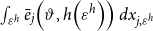 $\int _{\varepsilon ^{h}}\bar{e}_{j}\!\left (\vartheta,h\!\left(\varepsilon ^{h}\right)\right )dx_{j,\varepsilon ^{h}}$
, where
 $dx_{j,\varepsilon ^{h}}$
is the measure of the different health types of each age group in the population.
Finally, we calculate the average age-dependent conditional survival probability in the baseline calibration across the healthy and sick and then assign those probabilities to each age. Note that this adjustment automatically implies that the overall population size in this modified model is identical to that in the Baseline model.
With these specification changes in place, our No-health-risk model corresponds to the canonical rational-expectations overlapping generations framework that is routinely used to evaluate dynamic public policy but is augmented with a deterministic medical spending component to make it comparable (in terms of macro aggregates) to our Baseline model that includes idiosyncratic health risk. We do not otherwise re-calibrate this model, hence the benchmark outcomes between the model with and without health risk in Table 3 differ sl\rightly.
In all of our experiments, we measure the welfare effects using a consumption equivalence variation (CEV) measure, defined as a state-independent percentage change
 $\Delta _{C}$
in period consumption, such that the discounted expected lifetime utility under the experiment equals the discounted expected lifetime utility of the benchmark economy. Mathematically,
 $\Delta _{C}$
solves
 \begin{align} & \sum _{j=1}^{J}\mu _{j}\beta ^{j-1}\int \left [\begin{array}{c} \pi _{j}\!\left (h_{j}^{B}\!\left ({\textbf{\textit{x}}}_{j}^{B}\right )\right )\times u\!\left (\left (1+\Delta _{C}\right )\times c_{j}^{B}\!\left ({\textbf{\textit{x}}}_{j}^{B}\right ),n_{j}^{B}\!\left ({\textbf{\textit{x}}}_{j}^{B}\right );\,\bar{n}_{j}\cdot 1_{\left [n_{min}\leq n_{j}^{B}\!\left ({\textbf{\textit{x}}}_{j}^{B}\right )\right ]}\right )\\[9pt] +\beta \!\left (1-\pi _{j}\!\left (h_{j}^{B}\!\left ({\textbf{\textit{x}}}_{j}^{B}\right )\right )\right )\times b\!\left (a_{j+1}^{B}\right ) \end{array}\right ]d\Lambda \!\left ({\textbf{\textit{x}}}_{j}^{B}\right )\qquad\qquad\nonumber\\[5pt]& =\sum _{j=1}^{J}\mu _{j}\beta ^{j-1}\int \left [\begin{array}{c} \pi _{j}\!\left (h_{j}^{E}\!\left ({\textbf{\textit{x}}}_{j}^{E}\right )\right )\times u\!\left (c_{j}^{E}\!\left ({\textbf{\textit{x}}}_{j}^{E}\right ),n_{j}^{E}\!\left ({\textbf{\textit{x}}}_{j}^{E}\right );\,\bar{n}_{j}\cdot 1_{\left [n_{min}\leq n_{j}^{E}\!\left ({\textbf{\textit{x}}}_{j}^{E}\right )\right ]}\right )\\[9pt] \qquad\qquad\qquad + \beta \!\left (1-\pi _{j}\!\left (h_{j}^{E}\!\left ({\textbf{\textit{x}}}_{j}^{E}\right )\right )\right )\times b\!\left (a_{j+1}^{E}\right ) \end{array}\right ]d\Lambda \!\left ({\textbf{\textit{x}}}_{j}^{E}\right ), \qquad\qquad\end{align}
where superscripts
 $B$
and
 $E$
denote the baseline and the experiment, respectively. We also report separate CEV measures for each of the permanent income groups. Intuitively, this CEV measure captures the welfare gains (or losses) as percent of period consumption of a newly entering individual (i.e., a 25 year old in the model) under each one of our computational experiments.Footnote
19
We also examine the implications of these experiments for labor supply, consumption, and savings decisions, the markets for goods and services, the values of key macroeconomic aggregates, and the government’s budget.
5.1 Cutting Social Security’s payroll tax
First, what are the implications of the presence of health risk when attempting reforms such as cuts to Social Security? Our goal is to qualitatively and quantitatively asses the role of the health risk channel and how it interacts with the benefits and costs relevant for the program. To investigate this, we first reduce the payroll tax that funds Social Security from its baseline value of
 $\tau _{SS}=10.6$
% to
 $\tau _{SS}=5.3$
% (a reduction of 50%) while keeping the remaining institutional features fixed. We then adjust the scaling factor
 $a_{0}$
of the Social Security benefit-earnings formula (17) to clear the budget of the pension program in expression (2). This essentially reduces Social Security payments but retains the progressivity level of the payout formula. We run this experiment twice: first using the Baseline version of our model with full idiosyncratic health risk, and then using the No-health-risk version of our baseline model.
5.1.1 Payroll tax rate reduction with health risk
We report the results of this experiment for the Baseline version of our model in the second column of Table 4. It is clear from the table that not surprisingly, downsizing Social Security in our model environment leads to an overall welfare gain equivalent to
 $5.1$
% of period consumption, with larger welfare gains going to middle- and high-income households (CEVs of
 $+5.1$
% and
 $+6.8$
%, respectively). These welfare gains are driven primarily by increased labor supply and saving, which leads to an increase in labor and capital of roughly
 $3.4$
% and
 $6.6$
%, respectively. The effects on labor supply are driven by both labor participation (extensive margin) and labor hours of the working (intensive margin) across all three income groups. The increase in effective labor is sl\rightly stronger among the less educated who benefit the most from the increase of the overall wage rate of about
 $1.4$
%. In general, as we scale back Social Security, individuals increase their self-insurance efforts. First, due to lower payroll taxes, they have more disposable income, which is partly saved: capital owned by low- and middle-income households increase by
 $12$
and
 $11$
%, respectively. Second, higher wage rates ultimately induce workers to lower their labor hours as income effects overpower substitution effects. This leads to a decrease of the average labor hours of the working population from
 $39.1$
to
 $37.3$
hours per week.
Social Security tax cut by 50% with and without health risk

Notes: We simulate a 50% reduction of the size of Social Security in a model with idiosyncratic medical spending shocks and age deterministic health spending, respectively. The Health risk model has idiosyncratic health spending shocks and health affects labor productivity. The No-health-risk model has no idiosyncratic health spending shocks and income is independent of health. Medical spending in this model is deterministic and depends on age and the permanent income group. The magnitude of these age-dependent health expenditures is equal to the average health spending shock of the same age/permanent income type as in the model with full health risk. Due to the resulting lower variation in health spending, the Gini coefficient of health spending in the model without health risk is lower. We have not recalibrated the benchmark version of the no-risk model, therefore the benchmark versions of the two models shown above show sl\right differences in some of the aggregate moments. Data in rows marked with the % symbol are either fractions in percent or tax rates in percent. The other rows are normalized with values of the respective benchmark case. Each column presents steady-state results. CEV values are reported as percentage changes in terms of lifetime consumption of a newborn individual with respect to consumption levels in the benchmark. Labor No HiSchool, Labor HiSchool, and Labor College show the supply of efficiency units of labor for each agent type, respectively. Avge. Part. No HiSchool, Avge. Part. HiSchool, and Avge. Part. College shows the labor participation rate for each agent type respectively.
Social Security benefits of low- and middle-income households decrease by about
 $46$
% while the consumption insurance payments (referred to as Social Insurance at the bottom of Table 4) increase by 30% for low-income households. This is primarily the result of old, retired households in the lowest income group hitting the consumption floor due to the cuts to Social Security. On the other hand, consumption insurance payments to middle- and high-income groups drop as they are able to adequately save for retirement and thereby avoid the consumption floor. As a result, overall (Social Insurance) transfer payments decrease by about 7%. Despite the decreases in transfer payments, the growth effects are strong enough to result in overall welfare gains for the low- and medium-income households. High-income households experience a sl\rightly larger drop in their Social Security benefits (about 50.5% compared to 46% of the low- and middle-income groups), but due to the fact that these households are significantly more self-insured to begin with, their labor supply increases by only
 $1.9$
% and their capital stock decreases sl\rightly by
 $1.1$
%.
Since health expenditures are exogenous, the increase in capital stock causes an expansion in output and as a result we observe a decline of the medical expenditures to GDP ratio from
 $15.5$
to
 $14.9$
%. As one would expect, the Gini coefficient of asset holdings sl\rightly decreases as high-income households accumulate sl\rightly less capital than before the reduction in Social Security benefits. Due to the lower payroll tax, the Gini coefficient of labor income decreases sl\rightly as well. It is worth noting that the above welfare result (i.e., the observed welfare gain) is consistent with the fact that in a general equilibrium model with endogenous labor supply, Social Security’s distortionary welfare losses are larger than the welfare gains from partial insurance against labor income and mortality risk [Bagchi (Reference Bagchi2015)].Footnote
20
To summarize, downsizing Social Security allows households to better harness their precautionary motive and self-insure against health risk, and this effect is stronger for low- and middle-income households who are more likely to be borrowing constrained because of the Social Security payroll tax. We find that downsizing Social Security under the current benefit-earnings formula and taxable maximum for the Social Security payroll tax leads to welfare gains that are more pronounced for these households.
5.1.2 Payroll tax rate reduction in the absence of health risk
We next examine how a reduction in the size of Social Security affects welfare and the macro aggregates in the No-health-risk version of our model.Footnote
21
As before, we cut the Social Security payroll tax rate by 50% to
 $\tau _{SS}=5.3$
% and let the scaling parameter
 $a_{0}$
adjust to clear the Social Security budget in expression (2), while keeping the curvature parameter
 $a_{1}$
at its benchmark value.
Column 4 in Table 4 shows that similar to our baseline model, reducing the size of Social Security leads to a similar increase in capital of about
 $7.3$
%, which translates into a
 $4.5$
% increase in output. In this experiment, a newly entering individual experiences a welfare gain of
 $4.7$
% of compensating consumption. However, this welfare gain is smaller than what we find in our Baseline model under an identical tax cut. In other words, downsizing Social Security appears to have a smaller positive effect on welfare when we eliminate idiosyncratic health risk, which in turn suggests that Social Security allows better consumption smoothing in a model environment without health risk. Column 5 in Table 4 shows the difference (
 $\Delta$
) of the steady-state results of the model with idiosyncratic health risk (column 2) and the results of the model without idiosyncratic health risk (column 4).
Comparing the welfare effects of the payroll tax cut across permanent income groups, we find welfare gains equivalent to
 $3.3$
% and
 $4.7$
% of compensating consumption for low- and middle-income households, respectively, in our No-health-risk model, which are smaller than those obtained in our Baseline model. Clearly, these households do not benefit as much from Social Security’s insurance effects in the No-health-risk environment. High-income households, on the other hand, experience welfare gains equivalent to
 $6.9$
% of CEV in the No-health-risk environment, compared to
 $6.8$
% in the Baseline model. This should not be surprising, as Social Security leads to higher welfare losses among high-income households due to the progressivity of its payout formula. The presence of idiosyncratic health risk plays a smaller welfare role for high-income households as they can more effectively self-insure, with or without Social Security.
The capital accumulation rates increase for low- and middle-income households and decrease for high-income households, since these households were more likely to be borrowing constrained and had lower savings levels to begin with. Second, comparing the capital accumulation rates of the different household income types across the two models, we observe that in the model without idiosyncratic health risk the capital accumulation response is less elastic (i.e., low- and middle-income households accumulate less in the absence of idiosyncratic health risk, and high-income households decrease their capital stock less than in the model with health risk). The presence of health risk leads to stronger responses in capital accumulation in reaction to changes in the pension program.
In summary, we find that the presence of health risk in our model framework leads to an overall strengthening of the household-level precautionary motive, so downsizing Social Security leads to larger overall welfare gains. These welfare gains are more concentrated within low- and medium-income households, for whom health risk potentially poses a much larger consumption uncertainty. High-income households, on the other hand, also benefit from the payroll tax rate reduction, but their welfare gains are roughly identical both with and without health risk.
5.2 Modifying Social Security’s benefit-earnings formula
A key determinant of Social Security’s implicit insurance is the formula that governs the relationship between a household’s past work-life income and the level of Social Security benefits received during retirement. Currently, the US benefit-earnings formula replaces 90% of the average work-life earnings of households in the bottom 20% of the wage distribution but only about 40–50% of average work-life earnings of households with higher income. This concavity in the benefit-earnings rule is intended to facilitate better work-retirement consumption smoothing for households that m\right experience unfavorable health and labor income shocks during their work life. We now examine how health risk interacts with the welfare effects from modifying this benefit-earnings formula. We report the results from changing the curvature parameter
 $a_{1}$
in our baseline model with health risk and the model without health risk in Table 5.
Changing PIA progressivity
 $\textit{a}_{1}$
with and without health risk

Notes: We simulate a change in the progressivity level of the primary insurance amount (PIA) in a model with idiosyncratic medical spending shocks and age deterministic health spending, respectively. The Health risk model has idiosyncratic health spending shocks and health affects labor productivity. The No-health-risk model has no idiosyncratic health spending shocks and income is independent of health. Medical spending in this model is deterministic and depends on age and the permanent income group. The magnitude of these age-dependent health expenditures is equal to the average health spending shock of the same age/permanent income type as in the model with full health risk. Due to the resulting lower variation in health spending, the Gini coefficient of health spending in the model without health risk is lower. We have not recalibrated the benchmark version of the no-risk model, therefore the benchmark versions of the two models shown above show sl\right differences in some of the aggregate moments.
The middle column
 $\textit{a}_{1}\approx 0.57$
is the normalized benchmark economy with a PIA progressivity level based on US Social Security regulations. Data in rows marked with the % symbol are either fractions in percent or tax rates in percent. The other rows are normalized with values of the benchmark case (middle column). Each column presents steady-state results. CEV values are reported as percentage changes in terms of lifetime consumption of a newborn individual with respect to consumption levels in the benchmark. Labor No HiSchool, Labor HiSchool, and Labor College show the supply of efficiency units of labor for each agent type, respectively. Avge. Part. No HiSchool, Avge. Part. HiSchool, and Avge. Part. College shows the labor participation rate for each agent type, respectively.
5.2.1 Social Security progressivity with health risk
We first evaluate how changing the curvature of Social Security’s benefit-earnings rule affects welfare in our Baseline model with health risk. To do this, we recompute our model under Social Security’s curvature parameter values
 $a_{1}=0.0$
and
 $1.0$
in expression (17). Figure 6 shows the payout formula for various values of curvature parameter
 $a_{1}$
.
Social Security payout formula for different values of curvature parameter
 $\textit{a}_{1}$
. Notes: In these experiments
 $\textit{a}_{0}$
adjusts to clear the Social Security balance in expression (2). The benchmark parameters for the pension payout formula are
 $\textit{a}_0=2.214$
and
 $\textit{a}_1=0.567$
.

Functionally, parameter values
 $a_{1}=0$
and
 $a_{1}=1$
correspond to the two corner cases where Social Security benefits are either equal for all households and completely unrelated to past work-life income
 $(a_{1}=0),$
or where they are fully proportional (i.e., a linear function) to average work-life income
 $(a_{1}=1)$
. Also, note that in each experiment Social Security’s scale parameter
 $a_{0}$
adjusts to balance the Social Security budget constraint under the current payroll tax rate, the taxable maximum income, and the curvature parameter
 $a_{1}$
under that experiment according to expression (2).Footnote
22
The results for these experiments are summarized in columns 1–3 in Table 5.
5.2.2 Increasing PIA progressivity
 $(\textit{a}_{1}=0)$

As is clear from column 1 in Table 5, making Social Security’s benefit-earnings rule more progressive (decreasing
 $a_{1}$
) compared to the benchmark economy leads to a sharp drop in the Gini coefficient of Social Security payments from
 $0.26$
to
 $0.12$
and has an overall positive effect on welfare equivalent to a
 $2.95$
% percent increase in lifetime consumption.Footnote
23
The gains are largest at
 $6.2$
% of CEV for low-income households, but the change to lump-sum payments also generates losses of
 $0.5$
% of CEV for high-income households. We trace these welfare gains to two primary mechanisms that work in opposite direction:
 $\left (i\right )$
incentive effects, which reduce capital accumulation and lead to welfare losses, especially among high-income households, and
 $\left (ii\right )$
insurance effects, which produce welfare gains for low-income households.
First, the lump-sum pension payments trigger a negative effect on capital accumulation for low- and middle- income households as the promise of higher pension payments (increases of 16.8% and 5.2%, respectively) reduces household savings. We observe decreases in capital stock of almost 10% for low-income households and 3.5% for middle-income households. For high-income households the effect is reversed. The switch to a lump-sum pension payments effectively reduces the pension payments of high-income households by almost 25% so they respond by increasing their savings (capital stock increases by about 0.4%). Overall, this leads to a decrease in aggregate capital stock of
 $4.2$
% in our Baseline model with health risk. Wages decrease, average hours worked decrease, and the labor participation rate decreases across all three income groups. Overall, GDP decreases by 2.2%.
On the other hand, Social Security payments to low- and middle-income households increase so that fewer older households hit the consumption lower bound. Therefore, fewer older people require Social Insurance (e.g., food stamps) and we observe a drop in Social Insurance payments of over
 $40$
%. The decrease of labor and wages lead to lower incomes and since Social Security payments are indexed to income, the pension program shrinks, which counterbalances some of the negative incentive effects. However, the decrease in income, especially among the working population, leads to an almost
 $7.6$
% increase in overall Medicaid expenditures compared to an overall drop of Social Security payments of about
 $3.4$
%. From a public finance viewpoint this is an interesting result: a more equitable distribution of Social Security increases not only conditional transfers to the older poor population but also the younger poor population (through Medicaid). On the other hand, payments via the social insurance program—which maintains a minimum consumption floor and represents the other transfer program to the poor—decrease, seemingly because more equitable pension payments keep more individuals from hitting the consumption floor.
As the overall size of Social Security decreases by 3.4%, the size of Medicaid increases by about 7.6%. Without this increase, it stands to reason that low-income households may not have been able to gain from increased redistribution through the benefit-earnings rule of Social Security.
In summary, we observe that improved risk sharing through the more equitable Social Security system is welfare improving for households who experience relatively high income and health risk.Footnote 24 These households tend to have lower income which compromises their ability to self-insure, which is reflected in the observed welfare gains from a lump-sum benefit-earnings rule that is unrelated to past income. High-income households, on the other hand, experience welfare losses under this experiment, which ultimately turns Social Security into a more progressive program.
5.2.3 Decreasing PIA progressivity
$(\textit{a}_{1}=1)$

Making Social Security’s benefit-earnings rule less progressive (increasing
 $a_{1}$
) reduces the implicit redistribution through Social Security and leads to a welfare loss of
 $0.78$
% of CEV overall in our Baseline model with health risk. This is because with a linear (fully proportional) benefit-earnings rule, low- and medium-income households experience welfare losses equivalent to
 $3.1$
% and
 $0.8$
% of CEV, whereas high-income households gain from the fully proportional rule (CEV of
 $2.1$
%) as shown in Table 5.
With a linear payout formula, the pension system does not redistribute wealth between the permanent income groups as the returns from Social Security are proportional to the contributions to the program.Footnote
25
As a consequence, overall capital accumulation remains roughly unchanged as richer households can now recoup more of their pension contributions upon retirement. We observe this from the much higher Social Security payments to high-income households (an increase of almost
 $19$
%), which allows them to reduce their precautionary saving, thereby reducing their asset holdings by almost
 $3$
%. On the flip side, low- and middle-income households experience a drop in their Social Security benefits of almost
 $14$
% and 4%, respectively. Middle-income households save sl\rightly more to make up for the loss of insurance through Social Security, and low-income households do not change their savings that much due to negative income effects.
In addition, we observe that low- and middle-income households increase their labor supply. Not only do they increase their labor hours but they also increase their labor participation. Both are a reaction to the loss of insurance through pension payments and the need to work harder to generate additional funds that can be saved for retirement. The opposite holds for high-income households who cut back on labor hours worked. Overall, these labor market changes lead to sl\rightly lower wages. These negative income effects cause some of the low-income households to qualify for Medicaid which increases in size by
 $2.1$
%. Since high-income households save less now, they have enough funds to maintain their consumption levels despite negative income effects from lower wages. As a result, their welfare increases by
 $2.1$
%. Poorer households experience a relatively large welfare loss of almost
 $3.1$
% of CEV, which in a sense reverses the welfare results observed earlier under the earlier experiment.
5.2.4 Social Security progressivity in the absence of health risk
In order to investigate how much of the above welfare effects can be specifically attributed to the presence of idiosyncratic health spending risk, we next compute the above experiments with the No-health-risk version of our model.
5.2.5 Increasing PIA progressivity
$(\textit{a}_{1}=0)$

Even if idiosyncratic health risk is eliminated from our baseline model (No-health-risk version in Table 5), we find that switching to lump-sum benefits leads to an overall welfare gain equivalent to
 $2.66$
% of CEV, which is sl\rightly smaller than the
 $2.95$
% of CEV welfare gain in the Baseline model with health risk. This happens despite a
 $4.1$
% decrease in capital stock, which is sl\rightly smaller than the
 $4.2$
% decrease in the Baseline model. GDP decreases by
 $2.2$
% in this case, which is almost the same decrease we observed in the Baseline model under the same policy experiment. The welfare results are also very similar. Low-income households gain from the policy and high-income household lose. However, the magnitudes of the gains are sl\rightly larger (
 $6.67$
% vs.
 $6.16$
% for low-income households and
 $2.28$
% vs.
 $2.85$
% for middle-income households) as are the magnitudes of the losses (
 $-1.07$
% as compared to
 $-0.55$
%). As the precautionary savings motive is stronger in the model with idiosyncratic health risk, it is perhaps not surprising that a policy that provides insurance leads to smaller welfare gains in an environment where individuals have a strong incentive to self-insure compared to an environment where precautionary savings is less prevalent.Footnote
26
In summary, making Social Security’s benefit-earnings rule more progressive increases welfare, but the effect is stronger in the environment with health risk.
5.2.6 Decreasing PIA progressivity
$(\textit{a}_{1}=1)$

When we switch to a linear (fully proportional) benefit-earnings rule without health risk, we find that overall welfare decreases by
 $0.82$
% of CEV, with the largest welfare losses going to low-income households (CEV of
 $-3.1$
%). Middle-income households lose about
 $0.81$
% of CEV while high-income households gain about
 $2$
%. Comparing these to the welfare effects of the same experiment in our Baseline model, we find that decreasing the progressivity in Social Security’s benefit-earnings rule has roughly similar negative effect in the absence of health risk. In other words, the reduced insurance from a strictly proportional benefit-earnings rule appears to have largely the same effect in either scenario.
Decreasing the level of pension progressivity in the No-health-risk model increases capital stock by
 $0.34$
% which is sl\rightly smaller than the
 $0.35$
% increase in the Baseline model, and it also leads to an output gain of
 $0.61$
%, which is again sl\rightly smaller than the
 $0.62$
% decline in the Baseline model. Taken together, these results suggest that idiosyncratic health risk does not strongly affect the measured changes in aggregate variables under this experiment.
Finally, it is worth noting that the overall welfare effects of modifying Social Security’s benefit-earnings formula seem to suggest that additional insurance through a more progressive payout formula is welfare improving, especially for low- and middle-income households that are at a higher risk of ending up at the minimum consumption floor. In one of the earlier papers to investigate the insurance component of Social Security, Nishiyama and Smetters (Reference Nishiyama and Smetters2008) conclude that the long averaging period of US Social Security already provides substantial insurance against uninsured labor market risks, which suggests that additional insurance through a more concave benefit-earnings rule would be less important. We find evidence contrary to this result. Furthermore, if we make Social Security less progressive and move to a proportional benefit-earnings formula, our model predicts overall welfare losses despite the fact that high-income individuals would prefer a linear payout scheme over a lump-sum payout formula.
More recently, Bagchi (Reference Bagchi2019) examines how the positive correlation between income and life expectancy interacts with the welfare implications of Social Security’s benefit-earnings formula. Using a model with differential mortality but without health risk, he finds that the optimal benefit-earnings formula is sl\rightly less concave than the current US formula, because the poor have lower life expectancy and therefore they heavily discount the utility from old-age consumption. This appears to be not the case in our model: a more progressive Social Security payout formula leads to welfare gains, and this is true for the version with and without idiosyncratic health risk.
The key mechanisms that we capture in this paper that Nishiyama and Smetters (Reference Nishiyama and Smetters2008) and Bagchi (Reference Bagchi2019) ignore are the interactions of health risk with a household’s budget constraint as well as the households expected utility through a health-dependent survival process. Our model features three channels through which health risk affects households: their labor income, their medical expenditures, and also their life expectancy. Nishiyama and Smetters (Reference Nishiyama and Smetters2008) do not consider any of these channels in their welfare analysis of Social Security’s benefit-earnings rule, thereby underestimating the riskiness of the environment in which a household solves their life cycle problem. Bagchi (Reference Bagchi2019), on the other hand, accounts for differential mortality, that is, the positive correlation between income and life expectancy, but does not account for how labor income and medical expenditures are affected by a household’s exposure to health risk. Arguably, accounting for all of these channels together within a calibrated general equilibrium environment leads to somewhat different conclusions.
In our model, if we push toward a more progressive pension payments formula, then the presence of idiosyncratic health risk amplifies the welfare effects (i.e., gains) compared to an environment with health spending following a deterministic age-driven path. If we push toward a less progressive pension scheme, then the presence of idiosyncratic health risk dampens the welfare effects (i.e., losses). This finding that the insurance value of the program is higher when health risk is present is similar to the finding in Braun et al. (Reference Braun, Kopecky and Koreshkova2017) who show that the welfare benefits of mean-tested social insurance programs are larger when old-age Social Security is not available and vice versa. In addition, our result that moving to a lump-sum benefit formula is welfare improving is similar to the findings in Jones and Li (Reference Jones and Li2020) who show that welfare is maximized when baseline benefits of Social Security are independent of lifetime earnings.
5.3 Early Medicare
Given that the key mechanism in our model is the household-level precautionary motive, we next investigate how our computational results change when we allow households access to additional tools that help smooth health risk. One such tool is early Medicare eligibility (due to an event such as disability) that causes individuals to permanently exit the labor market before the traditional age of 65. The literature on early retirement has demonstrated a strong link of health shocks that lead to disability and subsequent early labor market exit [e.g., Low and Pistaferri (Reference Low and Pistaferri2015), Kitao (Reference Kitao2014), Blundell et al. (Reference Blundell, Britton, Dias and French2021)]. Disability Insurance (DI) therefore plays a key role for the early retirement decision of many individuals, especially in the 55 plus age range. The eligibility criteria for DI benefits and early Medicare payments are complex, so we focus on some of the key institutional details that capture the effects of accessing DI, Medicare, or Social Security before the age of 65. In particular, we modify our initial model to allow individuals to qualify for Medicare as early as age 55 and for Social Security as early as age 62 with the early collection penalties, both conditional on permanently exiting the labor market (thereby mimicking disability).Footnote 27 This extension, which we refer to as the “Early Medicare” model, introduces additional insurance against bad health shocks prior to the full retirement age. We repeat our two computational experiments, that is, cutting Social Security’s payroll tax by 50% and modifying the progressivity of the benefit-earnings rule, both with and without health risk, with this Early Medicare model.
As expected, we find that downsizing Social Security leads to roughly identical welfare gains both with and without health risk in this Early Medicare model (see Table 6). This is due to the fact that early Medicare allows households an additional tool to self-insure against bad health shocks that happen prior to age 65, as a result of which the precautionary motive is considerably weaker. The same is true when we modify the progressivity of Social Security’s benefit-earnings rule in this Early Medicare model (see Table 7): allowing for early Medicare, we find that the welfare gains from increased progressivity are roughly identical in models with and without health risk, and the welfare loss from reduced progressivity is significantly smaller in the presence of health risk.
Early retirement and Social Security tax cut by 50%

Notes: We simulate a 50% reduction of the size of Social Security in a model without early retirement benefits and a model with early retirement benefits. We again distinguish between a Health risk model with idiosyncratic health spending shocks and a No-health-risk model with deterministic age-dependent medical spending.
Early retirement and changing PIA progressivity
 $\textit{a}_{1}$

Notes: We simulate a change in the progressivity level of the primary insurance amount (PIA) in a model without early retirement benefits and a model with early retirement benefits. We again distinguish between a Health risk model with idiosyncratic health spending shocks and a No-health-risk model with deterministic age-dependent medical spending.
In summary, our computational results from the Early Medicare model suggest that the effects of the implementation details of the Social Security program (such as the magnitude of the payments or the progressivity of the payments) are not particularly sensitive to the presence of idiosyncratic health risk, if a different component of social insurance, such as a DI program, or in our case, Medicare benefits prior to the full retirement age of 65, already removes a large portion of this idiosyncratic risk.
6. Conclusions
In conclusion, in this paper we quantify the importance of idiosyncratic health risk in a calibrated general equilibrium model of Social Security. More specifically, we compare the welfare implications of Social Security in an environment with labor income, mortality, as well as health risks to those in an environment where health risk is removed from the model. To do this, we begin by constructing a calibrated general equilibrium macroeconomic model with households, firms, markets for goods and services, and a government that provides partial insurance against income and health risks. We then compute two experiments using this calibrated model.
First, in order to evaluate the overall consumption smoothing effects of Social Security, we compute the effects of a 50% reduction in Social Security’s payroll tax rate. Second, in order to examine how the degree of redistribution implicit in Social Security affects the welfare gains or losses for households with varying exposure to health risks, we compute the welfare effects of modifying the progressivity of Social Security’s benefit-earnings rule. Finally, we repeat these experiments in a hypothetical version of our model in which we remove health risk from the household’s economic environment. We also examine the implications of these experiments for labor supply, consumption, and saving decisions, the markets for goods and services, the values of key macroeconomic aggregates, and the government’s budget.
In general, our findings indicate that health risk has important implications for the welfare effects of Social Security. The presence of partially insured health risk, especially in old age, increases the consumption smoothing benefits of Social Security, but its payroll tax reduces disposable income in early life and negatively affects a household’s ability to self-insure against such risk. We find that in our model framework, the short-term consumption smoothing effect dominates: downsizing Social Security always leads to higher overall welfare in general equilibrium, but the welfare gain is larger when we account for health risk. We highl\right that in a riskier environment precautionary savings motives are stronger and the distortions caused by taxes and payouts related to the pension program are smaller. Downsizing a pension program that is less “distortive” to begin with therefore results in smaller welfare gains.
Similarly, we find that increasing the progressivity of Social Security’s benefit-earnings rule has a larger positive effect on overall welfare in the presence of health risk, and reduced progressivity has an almost identical negative effect both with and without health risk. In other words, our results from this experiment suggest that ignoring the effect of health risk on labor income, household expenditures, and survivorship in a general equilibrium environment underestimates the insurance value of Social Security.
Given that the key mechanism in our model is the trade-off between long- and short-term consumption smoothing, we also examine how our computational results change when we allow households access to additional tools that help smooth health risk, especially those that occur prior to the full retirement age of 65. To do this, we modify our initial model to allow individuals to qualify for Medicare as early as age 55 and for Social Security as early as age 62 with the early collection penalties, both conditional on permanently exiting the labor market. We find that as expected, downsizing Social Security leads to roughly identical welfare gains both with and without health risk in this case, and modifying the progressivity of Social Security’s benefit-earnings rule, welfare gains from increased progressivity are roughly identical with and without health risk, and the welfare loss from reduced progressivity is significantly smaller in the presence of health risk.
A key finding of this research addresses whether a quantitative policy analyst can safely ignore a careful representation of idiosyncratic health risk. The answer of whether idiosyncratic health risk matters for policy modeling depends on both
 $(i)$
the institutional details of the policy and
 $(ii)$
the households’ preference for consumption smoothing. For instance, we find large differences in the welfare effects between the health-risk and the No-health-risk models for the 50% Social Security tax cut when households’ level of risk aversion is moderate or high (
 $\sigma$
= 3 or 4). Similarly, we find large differences for models with high risk aversion when we modify the progressivity of Social Security’s benefit-earnings rule. In other words, if individuals are sufficiently risk averse, then including a careful representation of idiosyncratic health risk into the model framework is important, especially if the policy that a researcher attempts to simulate has a strong mitigating effect on this risk. If individuals are less risk averse and if the interested policy does not mitigate idiosyncratic health risk, then a model can abstract from including a careful representation of idiosyncratic health risk.
Finally, it is worth noting that we do not address the effects of transitions between the benchmark steady state and the new steady state under our counterfactual Social Security policies. Transition dynamics impose complex issues as they depend on the nature of the welfare criteria (e.g., welfare of newborn vs. welfare of different groups along transitions as discussed in Krueger and Ludwig (Reference Krueger and Ludwig2016)) as well as the way that the policy is phased in (e.g., a surprise one time implementation vs. staggered time varying implementations as discussed in Dyrda and Pedroni (Reference Dyrda and Pedroni2022)). While accounting for the costs of transitions is important for real-world policy evaluation in general [Bakıs et al. Reference Bakıs, Kaymak and Poschke2015, Krueger and Ludwig (Reference Krueger and Ludwig2016)], we conjecture that the interactions of idiosyncratic health risk with the workings of the Social Security program are unlikely to be affected by how a new Social Security policy is implemented. Moreover, due to the fact that our goal is to simply quantify the importance of such interactions rather than conducting comprehensive analyses of potential future policies, we leave the discussion of the effects of transitions in combination with the exposure to idiosyncratic health risk for future research. In addition, we also assume stable demographic patterns and exogenous health risk. Modeling an endogenous health capital investment process that affects survival and productivity is left for future research as are implementations of a human capital accumulation processes.
Supplementary material
To view supplementary material for this article, please visit http://doi.org/10.1017/S1365100522000438
Conflict of interest
Shantanu Bagchi received a Summer Research Grant from the College of Business and Economics at Towson University. Beyond that he has no further relevant or material financial interests that relate to the research described in this paper.
Juergen Jung received a grant from the School of Emerging Technologies (SET) at Towson University. Beyond that he has no further relevant or material financial interests that relate to the research described in this paper.
The content is solely the responsibility of the authors and does not represent the official views of the supporting institutions.