
1. Introduction
Historically, researchers have used the complex trajectories of particles in unsteady flows as a paradigm of chaotic motion. However, recent developments in coherent structure analysis has shifted focus away from characterizing the uncertainty in particle trajectories and towards discovering the foundational structures which determine their transport.
One central idea underlies much of this work: if organizing structures of particle transport are what are sought, then the particles themselves and their properties should be the best indicators of such structures. This motivates the approach pioneered by Haller & Yuan (Reference Haller and Yuan2000), where coherent structures are extracted by viewing the relationship between individual trajectories. More recently, this perspective has led to a proliferation of Lagrangian-based techniques for the detection of coherent structures, ranging from trajectories sampling deviations in flow conditions (Haller et al. Reference Haller, Hadjighasem, Farazmand and Huhn2016) to the network-based approaches of Schlueter-Kuck & Dabiri (Reference Schlueter-Kuck and Dabiri2017) and Hadjighasem et al. (Reference Hadjighasem, Karrasch, Teramoto and Haller2016).
In a sense, all of these techniques are data driven: structures are computed from viewing the trajectories after their transport by a dynamical system rather than from first principles. And although many of these approaches have seen success, it has been increasingly recognized that there are many issues in standard coherent structure analysis. As noted by Hadjighasem et al. (Reference Hadjighasem, Farazmand, Blazevski, Froyland and Haller2017), traditional methods have many free parameters which require significant tuning and often a priori knowledge of coherence to yield accurate results. Even techniques like spectral clustering, which claim fewer parameters (Hadjighasem et al. Reference Hadjighasem, Karrasch, Teramoto and Haller2016), are only straightforwardly applied to simple flows with well-defined trajectory clusters. As a result, some newer approaches have sought to minimize free parameters and establish firmer bases from which coherence can be judged. Filippi et al. (Reference Filippi, Rypina, Hadjighasem and Peacock2021), for example, introduces a form of spectral clustering which automatically selects optimal parameters using parameter sweeps to maximize the spectral gap of the eigenvalue spectrum. Other efforts, including that of Vieira, Rypina & Allshouse (Reference Vieira, Rypina and Allshouse2020), seek to quantify the uncertainty present in coherent structures analysis by altering user-provided parameters and observing the robustness of the results. And while these methods are successful in detecting structures most robust under advection by a flow, it is an attractive quality for the parameters of any coherent structure detection technique to have interpretability outside any particular flow. If the parameters or thresholds of an algorithm have physical meanings themselves, their values can be justified more generally and a priori before flow analysis, even in the event that the parameters themselves vary from case to case.
Even more dramatic, however, than the explosion of Lagrangian-based flow analyses has been the machine learning revolution, driven forward by the increasing availability of large data sets and the development of increasingly powerful algorithms for their analyses. Data-driven techniques have been used in the context of dynamical systems to reveal linear subspaces of highly nonlinear systems (Lusch, Kutz & Brunton Reference Lusch, Kutz and Brunton2018), to find governing equations given only trajectory information (Brunton et al. Reference Brunton, Proctor, Kutz and Bialek2016), and to identify underlying degrees of freedom in complex systems (Iten et al. Reference Iten, Metger, Wilming, Del Rio and Renner2020). Many parallels can be drawn between data from dynamical systems and, for example, the pixels of an image (Brunton, Noack & Koumoutsakos Reference Brunton, Noack and Koumoutsakos2020); it is unsurprising that as a result so many algorithms developed in the context of machine vision can be straightforwardly applied to large degree-of-freedom dynamical systems like those found in fluid mechanics.
In this paper we extend these ideas by analysing the spatial patterns which emerge when training a specialized neural network to reconstruct a large number of Lagrangian trajectories. In particular, by employing a neural network architecture known as an autoencoder, we show that when forced to communicate trajectory reconstruction information through noisy channels, neural networks will choose trajectories’ respective coherent structures as the most robust means of information transfer. This is not to say that we propose a more efficient or accurate means of generating coherent structures; rather, we explore the notion that a neural network will naturally ‘discover’ structures which strongly resemble those which have been well established, thereby adding an additional perspective to this body of work.
2. Robust representation
In any classical flow analysis it is often useful to seek a visualization of the flow in some non-trivial manner. To accomplish such a task in, for instance, a single two-dimensional image is actually quite challenging, as a large amount of information (say, an entire trajectory) must be represented in a single pixel (a scalar value). Streamlines may be sufficient for steady flows, but the behaviours of trajectories in even a simple unsteady flow already become difficult to communicate visually. For these complex flows, almost any image will fail to represent the full depth of trajectory dynamics. This is unsurprising: from a dimensional perspective, a trajectory sampled at  $N_t$ time points on some time interval will be a data point of dimension
 $d\times N_t$, where
 $d$ is the spatial dimension of the flow. To communicate the kinematics of trajectories in a single image, then, is to compress this
 $d\times N_t$ dimensional data point into a data point having just a single dimension.
We seek to view the Lagrangian coherent structure (LCS) problem as one of communication and representation. In other words, what are the simplest and most robust ways to communicate information about trajectories in a flow? If a single image is insufficient, how much information is really needed? In some sense, this is the basic strategy of LCS analysis in general: to seek the basic footprint which governs the Lagrangian nature of fluid elements. To extend our understanding of this broad field, and to explicitly relate the underlying structures to the accuracy of reconstructed Lagrangian trajectories, we turn to a machine learning framework known as an autoencoder.
2.1. Autoencoder (AE)
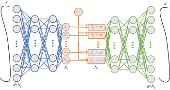
The basic set-up is simple: starting with a trajectory  $\boldsymbol{x}$ of dimension
 $d\times N_t$, a neural network transforms the data point through several connected layers into a vector
 $\boldsymbol {z}$ having only dimension
 $N_z$, where
 $N_z \ll d\times N_t$. Next, a second neural network must create a trajectory
 $x'$ resembling the original trajectory as well as possible, only by viewing the low-dimensional representation, the vector
 $\boldsymbol {z}$ with dimension
 $N_z$. We refer to each individual channel of this vector as
 $z_i$, where
 $i=1,2,\ldots ,N_z$. These two cooperating networks are known as the encoder and the decoder, respectively, and the low-dimensional vector is known as the latent layer or latent representation.
Since we seek robust, rather than simply sufficient representations, we include an extension to this basic framework. Rather than viewing the latent vector  $\boldsymbol {z}$ with channels
 $z_i$, the decoder instead sees a perturbed representation with channels
 $z_i+\sigma \epsilon$, where
 $\epsilon$ is Gaussian white noise. As a result of this set-up, the learned representation
 $\boldsymbol {z}$ must be robust to perturbations at least of size
 $\sigma$ or the decoder will fail to reconstruct the original trajectory. This set-up is shown in figure 1.
Schematic of the autoencoder framework we employ to reconstruct trajectories.

To finish the implementation of our autoencoder, we select as the loss function
 \begin{equation} L=\|\boldsymbol{x}-\boldsymbol{x}'\|^2+\beta\left[\frac{1}{N_z}\sum_{i=1}^{N_z}\mu_i^2\right], \end{equation}
which includes two distinct contributions. The first term,  $\|x-x'\|^2$, is a straightforward reconstruction loss which measures how closely the reconstructed trajectory
 $x'$ resembles the actual trajectory
 $x$. Since we fix the level of the Gaussian noise at
 $\sigma =1$, the network may train for arbitrarily large means so that the effects of noise are insignificant. In other words, with no penalty for the magnitude of the mean activation, the signal-to-noise ratio could become as large as necessary for accurate reconstructions. The second term in the loss function therefore penalizes this behaviour, and its relative strength in the loss formulation is controlled by the hyperparameter
 $\beta$, the value of which has been the subject of many studies (Higgins et al. Reference Higgins, Loic, Pal, Burgess, Glorot, Botvinick, Mohamed and Lerchner2017; Burgess et al. Reference Burgess, Higgins, Pal, Matthey, Watters, Desjardins and Lerchner2018). If
 $\beta =0$ the network can increase the signal-to-noise ratio and is only concerned with the accurate reconstruction of trajectories – not the robustness of the reconstructions towards noise. In this form the autoencoder is quite similar to a basic principle component analysis (PCA). In fact, a single layer autoencoder with no activation functions will learn the same coordinate transformation as PCA (Bengio, Courville & Vincent Reference Bengio, Courville and Vincent2013). As
 $\beta$ is increased, however, the network is subject to increasing levels of noise in the latent layer, and must become more clever about finding robust representations which the applied noise will not render unreadable by the decoder. In effect, the increase of
 $\beta$ decreases the signal-to-noise ratio in the latent representation, and is thus a parameter set by a user with a clearly defined and interpretable role in the physical system.
Our particular encoder is comprised of an input layer which takes as an input the coordinates of the trajectory, two hidden layers which contain 50 nodes each, and the latent layer with  $N_z$ nodes. All layers are fully connected and utilize ReLU (rectified linear unit) activation, except for the latent layer which uses an absolute value activation to ensure that the latent activations are positive. The architecture of the decoder is the same as the encoder, but reversed. Preliminary tests show that our results are robust to choices for the number of nodes in a network, but that certain choices like the activation function of the latent layer may influence the performance of the network.
3. Results
As LCS are known to control the transport of particles, we therefore expect them to feature prominently in the robust representation of trajectories in any such flow. To investigate this hypothesis, we choose two flows which have been the subject of previous coherent structure analysis: the unsteady Bickley jet and two-dimensional direct numerical simulation (DNS) of two-dimensional turbulence.
3.1. Bickley jet
The Bickley jet, an unsteady flow with distinct vortices and a central meandering jet, is defined on the domain  $x=[0,20]$ Mm and
 $y=[-3, 3]$ Mm by the streamfunction
 \begin{align} \varPsi(x,y,t)&=c_3y-U_0L\tanh(y/L) +A_3U_0L\mathrm{sech}^2(y/L)\cos(k_3x)\nonumber\\ &\quad+A_3U_0L\mathrm{sech}^2(y/L)\cos(k_2x-\sigma_2t). \end{align}
In the following analysis we follow the parameters of Rypina et al. (Reference Rypina, Brown, Beron-Vera, Koçak, Olascoaga and Udovydchenkov2007) and an integration time of  $T=10^6$ s. Choosing 10 latent nodes (
 $N_z=10$), we train the autoencoder architecture for ten distinct runs using values of
 $\beta$ logarithmically spaced between
 $\beta =0.001$ and
 $\beta =1.0$. These values of
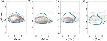
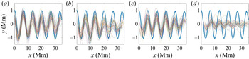
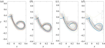
 $\beta$ represent increasing pressures for the network to communicate via robust representations under the influence of random noise, and decreasing relative pressures to reconstruct the trajectories accurately. Example reconstructed trajectories from the Bickley jet are shown in figures 2 and 3. As
 $\beta$ is increased, the reconstruction accuracy significantly suffers as expected. For trajectories within one of the vortices (figure 2), an increasing value of
 $\beta$ ultimately confuses the network such that it can no longer even qualitatively resemble the true dynamics. For a sample trajectory in the centre jet (figure 3), a similar degradation occurs with increasing
 $\beta$, but with some features retained in the reconstructed trajectories. In some sense this hints at a dynamic simplicity associated with the centre jet that is unlike any one of the vortices.
Example trajectory (in blue) taken from a vortex in the Bickley jet and attempts to reconstruct the trajectory by four different networks for training values of  $(a)$
 $\beta =0.001$,
 $(b)$
 $\beta =0.01$,
 $(c)$
 $\beta =0.1$ and
 $(d)$
 $\beta =1.0$.

Same as figure 2 but sample trajectory is taken from the central meandering jet.

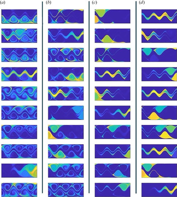
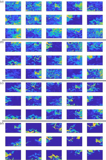
As with many dimensional reduction techniques, the reconstructed data are only part of the picture. Because the decoder can only see the representation of the latent layer, viewing these representations directly gives us insight into the essential flow features which are retained by the encoder – it is this process from which Lagrangian structures emerge. Since this autoencoder has  $N_z=10$ (a parameter choice whose effect is discussed below), each single trajectory will have some activation on all ten of the latent nodes. To visualize these activations, we apply the autoencoder to trajectories originating on an evenly spaced grid of initial conditions. In figure 4 we then show the mean activations
 $z_i$ of the latent layer. Here, each pixel of a latent node image represents the activation of a single trajectory starting in that particular initial position.
All  $N_{z} = 10$ latent nodes coloured by activated trajectories. Results are shown for
 $(a)$
 $\beta =0.001$,
 $(b)$
 $\beta =0.01$,
 $(c)$
 $\beta =0.1$ and
 $(d)$
 $\beta =1.0$. Each image corresponds to a single node.

Evident from figure 4, the learned representations of trajectories correspond well with the different dynamic regions of the Bickley jet, structures which have been thoroughly examined in previous studies (Hadjighasem et al. Reference Hadjighasem, Farazmand, Blazevski, Froyland and Haller2017). This is the explicit LCS connection that we sought from our method and a non-locality which departs from PCA. In figure 4 this is represented by the shift from the rightmost ( $\beta = 1.0$) to leftmost (
 $\beta = 0.001$) columns, where the node activations shift from ones which resemble LCS to those which resemble PCA. From the noise perspective, it makes sense to code dynamically similar trajectories (which are usually close to one another in physical space) into the same latent node. To illustrate: consider two trajectories, one belonging to a vortex and one belonging to the central jet (e.g. those in figures 2 and 3). If these two trajectories are coded into the same latent channel, added noise to the latent representation may lead to the confusion of one for the other and a large reconstruction loss. This very event is observed in figure 2(d), where a vortex trajectory is mistaken as one from the jet. So similar trajectories, often from the same dynamic region of the flow, are coded into nearby positions in the latent space using the same latent channel. This way, any noise added to the latent layer will only cause one vortex (jet) trajectory to be mistaken for another vortex (jet) trajectory and, therefore, a smaller reconstruction loss.
As a result of this interpretation, we can also view our method as related to that of Fang, Balasuriya & Ouellette (Reference Fang, Balasuriya and Ouellette2019) and Fang & Ouellette (Reference Fang and Ouellette2021). In these works, the authors define a coherent subset of a flow as a set of trajectories which can be constructed by linear approximations from one another. This definition tends to capture desirable properties of spatiotemporal coherence, and is connected to the operations performed by our autoencoder under the limit of large  $\beta$. Rather than defining similarity as the result of linear approximation, the latent layer reflects a richer notion of similarity as stemming from more general nonlinear transformations all related to the same kinds of kinematic motions, like that of a jet or that of a vortex.
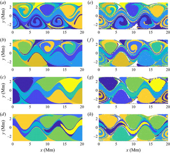
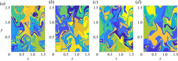
We demonstrate this result further in figure 5, where we colour each initial condition with the same colour if they activated the same latent node (therefore, there is a maximum of  $N_z$ possible colours). Then, we advect these nodes through the same training time length of the trajectories, since coherence under advection is generally a requirement among LCS techniques (Hadjighasem et al. Reference Hadjighasem, Farazmand, Blazevski, Froyland and Haller2017). Evident from figure 5, the structures detected in the high-noise limit of the Bickely jet are robust to advection at least within the time scale seen during training by the autoencoder. The opposite is true for the low-noise limit, as the critical structures retained by the autoencoder are subject to advection by the flow as would any random scalar field. The only exceptions to this observation are the coherent structures on the very edges of the initial domain. Because the autoencoder transformations are smooth in nature, the network struggles considerably to represent data on a periodic domain. For all training, therefore, trajectories are given to the encoder as continuous, so structures which are continuous on a periodic domain are nonetheless represented as two different structures.
Initial conditions of trajectories coloured by their corresponding latent node of highest activation. Results are shown for (a)  $\beta =0.001$, (b)
 $\beta =0.01$, (c)
 $\beta =0.1$ and (d)
 $\beta =1.0$. Advected final positions of trajectories for corresponding values of
 $\beta$ are shown in (e–h).

Now, a natural question is how the autoencoder behaves for a different number of latent nodes,  $N_z$. The entire point of dimensional reduction is to pass the trajectories through an information bottleneck, so excessively large values of
 $N_z$ eliminate the purpose of the endeavour altogether. Related to this is the question of what exactly the structures in figure 5 represent. In the present analysis we simply state that, for large
 $\beta$, these resemble the well-known LCS of the Bickley jet, and possess similar coherence properties under advection. However, they should not be expected to exactly align with LCS found by other techniques because this will be a function of
 $N_z$.
To pursue this line of inquiry, we repeat the training runs for two additional values of  $N_z=5$ and
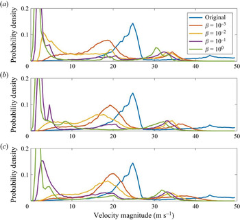
 $N_z=15$. As we have noted, it is challenging to determine an optimal number of coherent structures, as a single coherent structure can often be subdivided into two structures with the same level of coherence (this can be observed in figure 5). This a priori specification of the number of structures is a familiar problem with LCS methods in general. However, in the present context there is a limit in which too few latent nodes will not provide a sufficient amount of information to reconstruct flow features accurately. Figure 6 shows reconstructed probability density functions (p.d.f.s) of trajectory velocities for the three different networks trained on the Bickley jet. Evident from the reconstructed p.d.f.s, for all values of
 $N_z$, major flow features are retained (i.e. the large velocity magnitude peak which represents the meandering jet), and the accuracy with which these prominent flow features are reconstructed decreases with increasing values of
 $\beta$.
Reconstructed velocity p.d.f.s for  $(a)$
 $N_z=5$,
 $(b)$
 $N_z=10$ and
 $(c)$
 $N_z=15$.

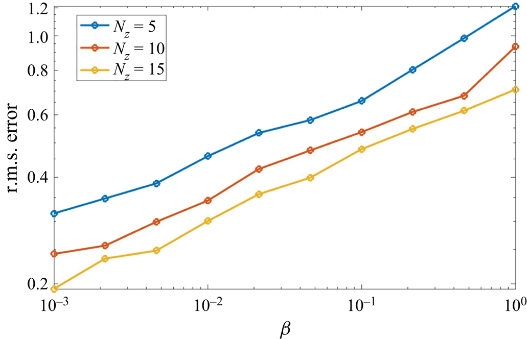
To quantify more precisely how this error scales with the noise in the latent layer, in figure 7 we plot the average root-mean-squared (r.m.s.) error against values of  $\beta$. Although different network architectures result in different average error for the same value of
 $\beta$, the relationship with which they scale remains constant. One interpretation of this behaviour is that the vertical position of this line reports information about the absolute level of accuracy, while the slope of the line indicates something more fundamental about the ease or difficulty of reconstructing trajectories in the flow in question. This interpretation makes the most sense when considering the limiting case: in a completely chaotic system with no spatiotemporal coherence, the autoencoder will not be able to extract any features. Increasing levels of noise will therefore have little effect on the reconstruction accuracy, as any change (regardless of magnitude) will have an equally negative influence on the autoencoder's ability to reconstruct trajectories. So, for a totally random system, we would expect that the reconstruction accuracy is independent of the latent noise
 $\beta$, or a flat line. The fact that all lines in figure 7 have generally the same slope for all
 $N_{z}$ reflects an underlying similarity between the network representations, and future efforts could therefore be focused on choosing
 $N_{z}$ according to the number or character of the coherent structures rather than overall reconstruction accuracy.
Root-mean-squared trajectory reconstruction error against latent layer noise  $\beta$ for the Bickley jet.

3.2. Two-dimensional turbulence
We now seek to demonstrate, briefly, that this method is not only useful for relatively simple problems like the Bickley jet. As done in other studies of LCS identification (Hadjighasem et al. Reference Hadjighasem, Farazmand, Blazevski, Froyland and Haller2017), we analyse DNS of two-dimensional turbulence. To generate the data, we solve the two-dimensional, incompressible Navier–Stokes equations on a periodic domain using a pseudospectral method. The flow is made turbulent by stochastic forcing, the exact set-up of which can be found in Karrasch & Schilling (Reference Karrasch and Schilling2020). We define a Reynolds number as  ${Re}=u_{{rms}}L/\nu$, where
 $u_{{rms}}$ is the r.m.s. velocity,
 $L$ is the length of the domain and
 $\nu$ is the kinematic viscosity. Our analysis will focus on a case at a Reynolds number of
 ${Re}=111$, but we also briefly consider a higher Reynolds number of
 ${Re}=255$.
As for our previous example, we train ten different networks at the same values of increasing  $\beta$. Because it is anticipated that there would be a greater number of underlying degrees of freedom in the flow, or a wider variety of coherent structures that could be identified, we start by training a network for
 $N_z=15$. Sample reconstructed trajectories for an integration length of
 $T=2$ s are shown in figure 8. Consistent with the results for the Bickley jet, as the hyperparameter
 $\beta$ is increased, the reconstruction fidelity decreases.

As  $\beta$ increases, the latent node activations also follow a similar pattern as before. Latent node colourings in the spirit of figure 4 are shown in figure 9. We again observe the trend that as the latent noise increases, node activations transition from local-in-energy structures towards local-in-space structures. By this we mean that for large
 $\beta$, initial locations which are close in physical space tend to activate together (local-in-space), whereas low values of
 $\beta$ cause more spatially disparate but energetic features (i.e. PCA) to be activated (local-in-energy). In correspondence with figure 5, figure 10 shows the trajectories coloured at their initial positions by the latent node of highest activation, and again we observe at the highest noise levels structures which strongly resemble LCS. It is worth noting, however, that some structures may be missing from these high-noise representations. Because the reconstruction loss is summed equally across all trajectories, highly coherent structures which contain a relatively small share of the trajectory ensemble are considered less important. As a result, structures like turbulent vortices are often included in some other latent representation, rather than in a latent node by themselves. As we have shown, in flows where vortices consist a large percentage of the trajectories (e.g. the Bickley jet), vortices are often represented in single latent nodes.
Same node colourings as figure 4 for (a)  $\beta =0.001$, (b)
 $\beta =0.01$, (c)
 $\beta =0.1$ and (d)
 $\beta =1.0$.

Same visualization as figure 5. As before, results are shown for (a)  $\beta =0.001$, (b)
 $\beta =0.01$, (c)
 $\beta =0.1$, (d)
 $\beta =1.0$.

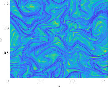
To solidify this interpretation, it is useful to compute the finite-time Lyapunov exponents (FTLEs) of the same system, the high-valued ridges of which separate dynamically distinct regions of a flow (see, for example, Shadden, Lekien & Marsden Reference Shadden, Lekien and Marsden2005). We begin by defining a flow map which maps trajectories from their initial positions  $x_0$ at time
 $t_0$ to their final positions
 $x_1$ at
 $t_1$,
 \begin{equation} \varPhi_{t_0}^{t_1}(x_0)=x_0+\int_{t_0}^{t_1}u(x,\tau)\,\textrm{d}\tau, \end{equation}
where  $u(x,t)$ is the velocity field of the flow. To understand the behaviour of these trajectories as their initial positions vary, we employ the Cauchy–Green strain tensor
 \begin{equation} \boldsymbol{\Delta} = [\nabla\varPhi_{t_0}^{t_1}]^{*}[\nabla\varPhi_{t_0}^{t_1}]. \end{equation}
The Cauchy–Green strain tensor offers a notion of how far initially close trajectories will stray over this time frame. This tensor then leads to the definition of the FTLE field as
 \begin{equation} \mathrm{FTLE}(x_0)=\frac{1}{t_1-t_0}\log(\sqrt{\lambda_{max}(\boldsymbol{\Delta})}), \end{equation}
where  $\lambda _{max}(\boldsymbol {\nabla })$ is the largest eigenvalue of
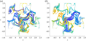
 $\boldsymbol {\nabla }$ and represents the largest separation that two trajectories advected under (3.2) will experience. Figure 11 shows the FTLE field computed for the same two-dimensional turbulence field. Comparing the ridges of the FTLE field with the boundaries of latent nodes in figure 10, we find strong correspondence for the highest noise levels (
 $\beta =1.0$). Furthermore, figure 12 shows the final positions of the advected tracers coloured by their latent node of highest activation for the lowest and highest noise levels. Because the ridges of the FTLE field separate regions of the flow where trajectories will diverge, we expect that the highest noise level structures will be most careful about separating trajectories along these lines. Indeed, we confirm that the trajectories in the high-noise limit are still spatially local, or coherent, after advection, whereas those for the low-noise limit are not.
Finite-time Lyapunov exponent field for the low-Reynolds-number two-dimensional turbulence.

Trajectories coloured by their latent node of highest activation for the lowest noise level  $\beta = 0.001$ (a) and highest noise level
 $\beta = 1.0$ (b).

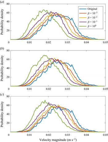
Finally, figure 13 shows the reconstructed p.d.f.s from networks with different values of  $N_z$. As before, we see consistent results across the different networks, indicating that the primary effect of
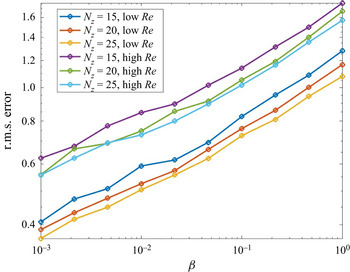
 $N_{z}$ in the present context is to perhaps unnecessarily split coherent structures into multiple segments. Interestingly, as the noise is increased for all networks, there is a bias towards lower velocities, but the error scales similarly for the different networks. Then in figure 14, we again plot the reconstruction error as a function of
 $\beta$. As in the case of the Bickley jet, the varying size of the latent layer causes the absolute reconstruction error to shift for a given value of
 $\beta$, but the fundamental rate at which error increases with increasing
 $\beta$ again remains roughly the same. To add to this, figure 14 also plots this relationship for the same flow but at a higher Reynolds number. At the larger
 ${Re}$, a jump in the r.m.s. error is seen, but interestingly, the rate at which the error rises with
 $\beta$ remains nearly constant. As suggested in the case of the Bickley jet, one interpretation of this behaviour is that the slope of this line indicates an underlying complexity of the flow – that is, how fundamentally difficult it is for the autoencoder network to reconstruct trajectories. Under this interpretation, there is a sense in which the two-dimensional turbulence at a higher Reynolds number is not necessarily a more complex flow, even if the errors themselves increase in an absolute sense. We defer this question to future analysis.
Reconstructed velocity p.d.f.s for (a)  $N_z=15$, (b)
 $N_z=20$ and (c)
 $N_z=25$.

Root-mean-squared error against latent layer noise  $\beta$ for two-dimensional turbulence at two different Reynolds numbers.

4. Conclusion
Utilizing the machine learning framework known as an autoencoder, we demonstrate that the most robust way to encode information about trajectories is through their respective coherent structures – one which can span from traditional PCA to more complex LCS based on a signal-to-noise hyperparameter  $\beta$. This parameter comes with an intuitive interpretation – acceptable reconstruction loss – the selection of which is motivated outside of a posteriori validation and can be chosen differently in different circumstances. For low values of
 $\beta$, node activations resemble local-in-energy coherent structures, since this limit naturally seeks the most energetic features of the flow, even if these are non-local in physical space. In the limit of high
 $\beta$, the presence of noise forces the autoencoder network to seek more robust features to maintain trajectory accuracy, and what we observe strongly resembles the well-known LCS for both the Bickley jet and two-dimensional turbulence.
There is still much to be explored about the connection between robust representation of trajectories and coherent structures. For example, this method is still dependent on setting the number of latent nodes ahead of time, unnecessarily fragmenting coherent structures across multiple nodes. Preliminary work has shown promise of employing a variational autoencoder, where the noise level is also a learned parameter, since this in theory forces the network to limit the number of activated nodes. This is an interesting avenue for future research. Another avenue for continued research is the relationship between trajectory reconstruction error and  $\beta$, since our results suggest that this provides an indication of the underlying complexity of the flow.
Funding
The authors acknowledge grant G00003613-ArmyW911NF-17-0366 from the US Army Research Office and grant N00014-18-1-2472 from the US Office of Naval Research. Computational resources were provided by the Center for Research Computing (CRC) at the University of Notre Dame.
Declaration of interests
The authors report no conflict of interest.