2.1 Solving the two free-boundary problems

The algorithm presented in Galeano-Rios et al. (Reference Galeano-Rios, Milewski and Vanden-Broeck2017) solves the problem of the suddenly appearing pressed area and its subsequent evolution upon the impact of a solid. Moreover, the method is able to deal with the vanishing contact area when lift-off takes place. We review it in what follows. We first consider, for simplicity, the solid to be fixed as the free surface impacts on it. That is to say, we consider the case of $h(t)$ being constant and solving the system given by (2.1)–(2.11), disregarding (2.7) initially. We then discuss how (2.7) is introduced.

Figure 1.

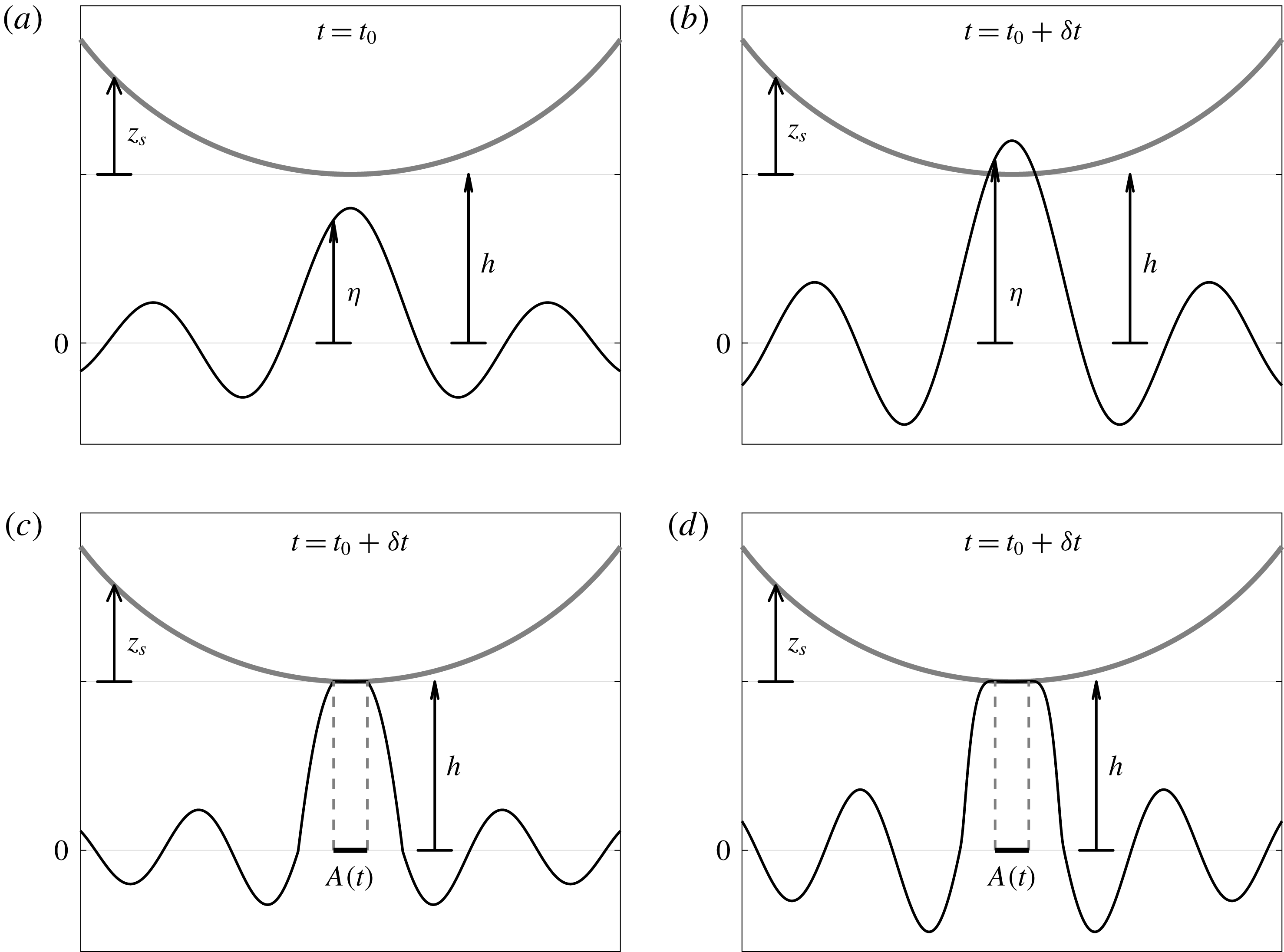
Schematics of onset of contact as solved by the kinematic match method. The boundary of the fixed solid, given by $z_{s}$ , is shown in grey; and the fluid interface, given by $\unicode[STIX]{x1D702}$ , in black. The height of the solid surface $z_{s}$ is measured with respect to that of its lowest point $h$ . Panels show: (a) regular evolution with no pressed area, (b) inconsistent estimate of free surface at $t=t_{0}+\unicode[STIX]{x1D6FF}t$ , (c) tentative solution for $t=t_{0}+\unicode[STIX]{x1D6FF}t$ with an $A_{test}$ that yields a wrong contact angle, and (d) solution with an $A_{test}$ that yields the right contact angle.

We consider the free surface of a fluid bath which, at a time $t=t_{0}$ , approaches a fixed, perfectly hydrophobic solid, shown in figure 1(a). In order to calculate the free-surface elevation at a certain time $t_{0}+\unicode[STIX]{x1D6FF}t$ , we need to solve the free-boundary problem over the time interval $t\in [t_{0},t_{0}+\unicode[STIX]{x1D6FF}t]$ . First, we tentatively impose $p_{s}(\boldsymbol{x},t)=0$ and we solve the system given by (2.1)–(2.6); if the solution satisfies (2.10) everywhere (i.e. predicts no contact or overlap between the fluid and the solid), then it trivially solves the remaining conditions of system (2.1)–(2.11). However, if (as in the example of figure 1) our prediction for the location of the free surface at time $t_{0}+\unicode[STIX]{x1D6FF}t$ suggests that part of the fluid occupies the same space as the solid, then we have not obtained a solution to (2.1)–(2.11) and an impact must have occurred; see figure 1(b). The evolution of the free surface should have been constrained by the presence of the solid and there should be a region within which $p_{s}(\boldsymbol{x},t)$ was not identically zero over the interval $[t_{0},t_{0}+\unicode[STIX]{x1D6FF}t]$ .

In order to find a correct solution to system (2.1)–(2.11), and since $A(t_{0}+\unicode[STIX]{x1D6FF}t)$ is to be determined, we proceed by testing a contact area candidate $A_{test}$ . We assume the contact area changes continuously; therefore $A_{test}$ must be small at the onset of contact. We solve the system for $\unicode[STIX]{x1D702}$ everywhere outside $A_{test}$ , and for the value of $p_{s}$ on $A_{test}$ (where $\unicode[STIX]{x1D702}$ is known). The method exchanges the known and unknown variables in the pressed area, yielding a closed problem for system (2.1)–(2.9) at $t_{0}+\unicode[STIX]{x1D6FF}t$ . Naturally, the solution to (2.1)–(2.9), obtained assuming $A(t+\unicode[STIX]{x1D6FF}t)=A_{test}$ , might not satisfy (2.10) or (2.11), since this was just an initial choice, so we need to verify these. If either condition is not satisfied, we repeat the process using a new $A_{test}$ , obtained by perturbing our prior choice until the solution satisfies (2.10) and (2.11) (see figures 1(c) and 1(d)).

At a time $t=t_{1}$ , when the fluid is in contact with the solid (i.e. $A(t_{1})\neq \emptyset$ ), we proceed with the method in a similar manner. For time $t_{1}+\unicode[STIX]{x1D6FF}t$ we iterate on our candidate pressed areas $A_{test}$ , chosen in the vicinity of $A(t_{1})$ , and we solve system (2.1)–(2.9) for each $A_{test}$ until we verify (2.10) and (2.11). We note that, if $A(t_{1})$ is relatively small, the empty set is considered to be in its vicinity and therefore we include the possibility of $A_{test}=\emptyset$ , i.e. $p_{s}(\boldsymbol{x},t)=0$ .

When the impacting object is able to move vertically, the problem involves the response of the fluid forces onto it and we still need to iterate on the contact area; however, we no longer know a priori the exact elevation of the free surface $\unicode[STIX]{x1D702}$ on $A_{test}$ . Nevertheless, we know $\unicode[STIX]{x1D702}$ up to a vertical translation, given by $h(t)$ . This vertical translation adds an unknown to the system, but we also add (2.7), which closes the problem (2.1)–(2.9) for a given $A_{test}$ at $t=t_{0}+\unicode[STIX]{x1D6FF}t$ . We can thus iterate on $A_{test}$ once again, and stop the iteration when (2.10) and (2.11) are satisfied.

2.2 The linearised model

2.2.1 Linearised fluid equations

Following Galeano-Rios et al. (Reference Galeano-Rios, Milewski and Vanden-Broeck2017) we use a linearised quasi-potential approximation of the fluid flow, with $\boldsymbol{u}$ defined on the domain $D=\{(\boldsymbol{x},z),z\leqslant 0\}$ , where $z=0$ is the undisturbed free-surface level. We define $\unicode[STIX]{x1D711}(\boldsymbol{x},z,t)$ as the velocity potential, $\unicode[STIX]{x1D6E5}_{H}$ as the two-dimensional Laplacian, i.e. $\unicode[STIX]{x1D6E5}_{H}=\unicode[STIX]{x2202}_{xx}+\unicode[STIX]{x2202}_{yy}$ , and $N$ as the Dirichlet-to-Neumann operator, given by

(2.12) $$\begin{eqnarray}\displaystyle N\unicode[STIX]{x1D711}(\boldsymbol{x},0,t)=\unicode[STIX]{x1D711}_{z}(\boldsymbol{x},0,t). & & \displaystyle\end{eqnarray}$$

In formulating the Faraday wave problem, we set $g$ as the gravity constant, $a$ as the amplitude of the vertical shaking and $\unicode[STIX]{x1D714}_{o}$ as its angular frequency. The fluid viscosity $\unicode[STIX]{x1D708}$ is corrected to $\unicode[STIX]{x1D708}^{\ast }$ in order to use a quasi-potential approximation whilst still matching the driving amplitude at which the Faraday threshold is observed. For the parameter regime at which we run simulations (see appendix A), $\unicode[STIX]{x1D708}^{\ast }=0.8025\unicode[STIX]{x1D708}$ (Milewski et al. Reference Milewski, Galeano-Rios, Nachbin and Bush2015). We adopt the Faraday wavelength $\unicode[STIX]{x1D706}_{F}$ as the unit length, the reciprocal of the subharmonic Faraday wave frequency $f_{F}^{-1}$ as the unit time, and $\unicode[STIX]{x1D70C}\unicode[STIX]{x1D706}_{F}^{3}$ as the unit mass, where $\unicode[STIX]{x1D70C}$ is the density of the bath’s fluid. We also define

(2.13a-d ) $$\begin{eqnarray}\displaystyle Fr=\unicode[STIX]{x1D706}_{F}\,f_{F}^{2}/g,\quad We=\unicode[STIX]{x1D70C}\unicode[STIX]{x1D706}_{F}^{3}\,f_{F}^{2}/\unicode[STIX]{x1D70E},\quad \unicode[STIX]{x1D6E4}=a\unicode[STIX]{x1D714}_{o}^{2}/g,\quad Re=\unicode[STIX]{x1D706}_{F}^{2}\,f_{F}/\unicode[STIX]{x1D708}^{\ast }, & & \displaystyle\end{eqnarray}$$

and $\unicode[STIX]{x1D719}(\boldsymbol{x},t)=\unicode[STIX]{x1D711}(\boldsymbol{x},0,t)$ .

The free surface can be shown to evolve (Galeano-Rios et al. Reference Galeano-Rios, Milewski and Vanden-Broeck2017) according to

(2.14) $$\begin{eqnarray}\displaystyle & \displaystyle \unicode[STIX]{x1D702}_{t}={\displaystyle \frac{2}{Re}}\unicode[STIX]{x1D6E5}_{H}\unicode[STIX]{x1D702}+N\unicode[STIX]{x1D719}, & \displaystyle\end{eqnarray}$$

(2.15) $$\begin{eqnarray}\displaystyle & \displaystyle \unicode[STIX]{x1D719}_{t}=-{\displaystyle \frac{(1-\unicode[STIX]{x1D6E4}\cos (4\unicode[STIX]{x03C0}t))}{Fr}}\unicode[STIX]{x1D702}+{\displaystyle \frac{1}{We}}\unicode[STIX]{x1D705}[\unicode[STIX]{x1D702}]+{\displaystyle \frac{2}{Re}}\unicode[STIX]{x1D6E5}_{H}\unicode[STIX]{x1D719}-p_{s}, & \displaystyle\end{eqnarray}$$

subject to

(2.16) $$\begin{eqnarray}\displaystyle & \displaystyle \unicode[STIX]{x1D702}\rightarrow 0,\quad \text{when }\sqrt{x^{2}+y^{2}}\rightarrow \infty , & \displaystyle\end{eqnarray}$$

(2.17) $$\begin{eqnarray}\displaystyle & \displaystyle \unicode[STIX]{x1D719}\rightarrow 0,\quad \text{when }\sqrt{x^{2}+z^{2}}\rightarrow \infty . & \displaystyle\end{eqnarray}$$

We note that these equations describe the free surface in the frame of reference of the moving bath, which introduces a time-dependent coefficient in (2.15), and that the curvature $\unicode[STIX]{x1D705}$ is not yet linearised. In fact, we will retain the full curvature in the contact area, where it is $O(1)$ and known a priori from the geometry of the solid, as was done in Galeano-Rios et al. (Reference Galeano-Rios, Milewski and Vanden-Broeck2017).

2.2.2 Vertical dynamics of the sphere

We recall that $m_{s}$ is the mass of the droplet and define $\unicode[STIX]{x1D707}_{air}$ as the dynamic viscosity of air, $R_{o}$ as the droplet radius and $h^{c}$ as the height of the centre of mass, which yields $h=(h^{c}-R_{o})/\unicode[STIX]{x1D706}_{F}$ as the dimensionless height of the south pole of the sphere. We approximate the effects of air on the moving droplet using Stokes’ drag and we introduce the dimensionless quantities

(2.18a,b ) $$\begin{eqnarray}\displaystyle Ma=m_{s}/(\unicode[STIX]{x1D70C}\unicode[STIX]{x1D706}_{F}^{3}),\quad So=6\unicode[STIX]{x03C0}\unicode[STIX]{x1D707}_{air}R_{o}/(m_{s}\,f_{F}). & & \displaystyle\end{eqnarray}$$

We thus have

(2.19) $$\begin{eqnarray}\displaystyle h_{tt}=-{\displaystyle \frac{(1-\unicode[STIX]{x1D6E4}\cos (4\unicode[STIX]{x03C0}t))}{Fr}}-So\,h_{t}+{\displaystyle \frac{1}{Ma}}\int _{A(t)}p_{s}\,\text{d}A. & & \displaystyle\end{eqnarray}$$

We describe the lower half of the impacting sphere, in dimensionless variables, using

(2.20) $$\begin{eqnarray}\displaystyle z_{s}(\boldsymbol{x})=\left\{\begin{array}{@{}ll@{}}{\displaystyle \frac{R_{o}}{\unicode[STIX]{x1D706}_{F}}}-\sqrt{{\displaystyle \frac{R_{o}^{2}}{\unicode[STIX]{x1D706}_{F}^{2}}}-|\boldsymbol{x}|^{2}}, & |\boldsymbol{x}|\leqslant {\displaystyle \frac{R_{o}}{\unicode[STIX]{x1D706}_{F}}},\\[6.0pt] \infty , & |\boldsymbol{x}|>{\displaystyle \frac{R_{o}}{\unicode[STIX]{x1D706}_{F}}}.\end{array}\right. & & \displaystyle\end{eqnarray}$$

Thus, given the horizontal location of the centre of mass as $\boldsymbol{X}(t)=(X(t),Y(t))$ , we can rewrite constraints (2.8)–(2.11) as

(2.21) $$\begin{eqnarray}\displaystyle & \displaystyle p_{s}=0,\quad \boldsymbol{x}\notin A(t), & \displaystyle\end{eqnarray}$$

(2.22) $$\begin{eqnarray}\displaystyle & \displaystyle \unicode[STIX]{x1D702}(\boldsymbol{x},t)=h(t)+z_{s}(\boldsymbol{x}-\boldsymbol{X}(t)),\quad \boldsymbol{x}\in A(t), & \displaystyle\end{eqnarray}$$

(2.23) $$\begin{eqnarray}\displaystyle & \displaystyle \unicode[STIX]{x1D702}(\boldsymbol{x},t)<h(t)+z_{s}(\boldsymbol{x}-\boldsymbol{X}(t)),\quad \boldsymbol{x}\notin A(t), & \displaystyle\end{eqnarray}$$

(2.24) $$\begin{eqnarray}\displaystyle & \displaystyle \unicode[STIX]{x2202}_{n}\unicode[STIX]{x1D702}(\boldsymbol{x},t)=\unicode[STIX]{x2202}_{n}z_{s}(\boldsymbol{x}-\boldsymbol{X}(t)),\quad \boldsymbol{x}\in L(t). & \displaystyle\end{eqnarray}$$

The horizontal trajectory $\boldsymbol{X}(t)$ is naturally dependent on the surface waves, and it needs to be coupled to system (2.14)–(2.24) to close the problem. For the sake of clarity, we present the horizontal dynamics in detail later in the text.

We highlight that, whilst the problem given by (2.14)–(2.24) is linear during each droplet flight, the problem remains highly nonlinear during impacts. The implicit nonlinearity takes place through the free-boundary problem for the pressure and the pressed area.

2.3 Approximation by superposition of normal impacts

We now introduce a further approximation to the problem, namely we consider impacts to be quasi-normal to the surface. This approximation was used by all previous works on walking droplets; however, the arguments that follow constitute (to the best of our knowledge) the first mathematical justification for it.

As mentioned in § 1, the walking velocity of droplets ( $C_{w}\approx 1~\text{cm}~\text{s}^{-1}$ ) is typically small relative to the vertical velocity of impact ( $U_{z}\approx 10~\text{cm}~\text{s}^{-1}$ ). This means that impacts are nearly vertical and that the difference between imposing condition (2.22) exactly and approximately (i.e. using the simplification that $\boldsymbol{X}(t)$ is constant during the impact) is of the order of the distance that the droplet moved during contact with the bath multiplied by the gradient of $z_{s}$ (bottom half of a sphere). Moreover, the linear approximation to surface deflection allows for the problem to be decomposed into a vertical (i.e. almost normal) impact on an initially quiescent interface and the unforced evolution of the waves.

We consider the time $t=t_{0}$ at which impact is imminent and we rewrite equation (2.22), in dimensionless units, as for $t\in (t_{0},t_{l})$ :

(2.25) $$\begin{eqnarray}\displaystyle \unicode[STIX]{x1D702}(\boldsymbol{x},t)=h(t)+z_{s}(\boldsymbol{x}-\boldsymbol{X}(t_{0}))+[z_{s}(\boldsymbol{x}-\boldsymbol{X}(t))-z_{s}(\boldsymbol{x}-\boldsymbol{X}(t_{0}))],\quad \boldsymbol{x}\in A(t). & & \displaystyle\end{eqnarray}$$

Here we know the term in square brackets to be of $O(|\unicode[STIX]{x1D735}z_{s}|C_{w}(t_{l}-t_{0})/\unicode[STIX]{x1D706}_{F})$ , where $t_{l}$ is the time at which lift-off happens with $t_{l}-t_{0}<T_{F}/2$ (typically), and $C_{w}$ is the typical speed of a walking droplet, which is small with respect to the phase velocity of the waves, $C_{p}=\unicode[STIX]{x1D706}_{F}/T_{F}$ . Moreover, for the case of an impacting sphere, when the radius of $A(t)$ is less than half the radius of the sphere (as is the typical case for walking droplets), $|\unicode[STIX]{x1D735}z_{s}|$ is at most $O(1)$ . Therefore, the term in square brackets is at most $O(C_{w}/C_{p})$ (typically $C_{w}/C_{p}\approx 0.05$ ) and thus we can conclude that, near the impact location, we can impose an axisymmetric kinematic condition (by ignoring the term in square brackets) with an error of at most this order.

We now rewrite the quasi-normal impact as the superposition of three different problems: problem $a$ , given by the axisymmetric impact of a sphere onto the quiescent surface of a bath; problem $b$ , defined by the unforced wave field evolution of the free surface without the ongoing impact; and problem $r$ , given by the remaining terms in the full problem. More specifically, we define problems $a$ and $b$ , such that

(2.26) $$\begin{eqnarray}\displaystyle & \displaystyle \unicode[STIX]{x1D702}=\unicode[STIX]{x1D702}^{a}+\unicode[STIX]{x1D702}^{b}+\unicode[STIX]{x1D702}^{r}, & \displaystyle\end{eqnarray}$$

(2.27) $$\begin{eqnarray}\displaystyle & \displaystyle \unicode[STIX]{x1D719}=\unicode[STIX]{x1D719}^{a}+\unicode[STIX]{x1D719}^{b}+\unicode[STIX]{x1D719}^{r}, & \displaystyle\end{eqnarray}$$

(2.28) $$\begin{eqnarray}\displaystyle & \displaystyle h(t)=h^{a}(t)+\unicode[STIX]{x1D702}^{b}(\boldsymbol{X}(t),t)+h^{r}(t), & \displaystyle\end{eqnarray}$$

where the super-indices $a$ and $b$ indicate the solution of each problem and $r$ is the remainder with respect to the solution of the full impact problem (2.14)–(2.24). First, for $t\in [t_{0},t_{l}]$ , we define the homogeneous problem $b$ as

(2.29) $$\begin{eqnarray}\displaystyle & \displaystyle \unicode[STIX]{x1D702}_{t}^{b}={\displaystyle \frac{2}{Re}}\unicode[STIX]{x1D6E5}_{H}\unicode[STIX]{x1D702}^{b}+N\unicode[STIX]{x1D719}^{b}, & \displaystyle\end{eqnarray}$$

(2.30) $$\begin{eqnarray}\displaystyle & \displaystyle \unicode[STIX]{x1D719}_{t}^{b}=-{\displaystyle \frac{(1-\unicode[STIX]{x1D6E4}\cos (4\unicode[STIX]{x03C0}t))}{Fr}}\unicode[STIX]{x1D702}^{b}+{\displaystyle \frac{1}{We}}\unicode[STIX]{x1D6E5}_{H}\unicode[STIX]{x1D702}^{b}+{\displaystyle \frac{2}{Re}}\unicode[STIX]{x1D6E5}_{H}\unicode[STIX]{x1D719}^{b}, & \displaystyle\end{eqnarray}$$

subject to $\unicode[STIX]{x1D702}^{b}$ , $\unicode[STIX]{x1D719}^{b}\rightarrow 0$ when $|x|\rightarrow \infty$ , with

(2.31a,b ) $$\begin{eqnarray}\displaystyle \unicode[STIX]{x1D702}^{b}(\boldsymbol{x},t_{0})=\unicode[STIX]{x1D702}(\boldsymbol{x},t_{0})\quad \text{and}\quad \unicode[STIX]{x1D719}^{b}(\boldsymbol{x},t_{0})=\unicode[STIX]{x1D719}(\boldsymbol{x},t_{0}). & & \displaystyle\end{eqnarray}$$

That is to say, problem $b$ gives the evolution of the fluid flow as if the impact that occurs in the time interval $[t_{0},t_{l}]$ does not take place. We highlight that, due to the finite wave speed, outside the vicinity of the impact location, problem $b$ is in fact the full problem.

We can then rewrite equation (2.25) using equation (2.26) and subtract $\unicode[STIX]{x1D702}^{b}(\boldsymbol{X}(t),t)$ from both sides to obtain

(2.32) $$\begin{eqnarray}\displaystyle & & \displaystyle \unicode[STIX]{x1D702}^{a}(\boldsymbol{x},t)+[\unicode[STIX]{x1D702}^{b}(\boldsymbol{x},t)-\unicode[STIX]{x1D702}^{b}(\boldsymbol{X}(t),t)]+\unicode[STIX]{x1D702}^{r}(\boldsymbol{x},t)\nonumber\\ \displaystyle & & \displaystyle \quad =[h(t)-\unicode[STIX]{x1D702}^{b}(\boldsymbol{X}(t),t)]+z_{s}(\boldsymbol{x}-\boldsymbol{X}(t_{0}))+O(C_{w}/C_{p}),\end{eqnarray}$$

where the term in square brackets on the right-hand side of (2.32) will be used to define $h^{a}$ as used in (2.28). Namely, for $t\in [t_{0},t_{l}]$ , we define the axisymmetric impact problem $a$ as

(2.33) $$\begin{eqnarray}\displaystyle & \displaystyle \unicode[STIX]{x1D702}_{t}^{a}={\displaystyle \frac{2}{Re}}\unicode[STIX]{x1D6E5}_{H}\unicode[STIX]{x1D702}^{a}+N\unicode[STIX]{x1D719}^{a}, & \displaystyle\end{eqnarray}$$

(2.34) $$\begin{eqnarray}\displaystyle & \displaystyle \unicode[STIX]{x1D719}_{t}^{a}=-{\displaystyle \frac{(1-\unicode[STIX]{x1D6E4}\cos (\unicode[STIX]{x1D714}_{o}t))}{Fr}}\unicode[STIX]{x1D702}^{a}+{\displaystyle \frac{1}{We}}\unicode[STIX]{x1D705}[\unicode[STIX]{x1D702}^{a}]+{\displaystyle \frac{2}{Re}}\unicode[STIX]{x1D6E5}_{H}\unicode[STIX]{x1D719}^{a}-p_{s}^{a}, & \displaystyle\end{eqnarray}$$

(2.35) $$\begin{eqnarray}\displaystyle & \displaystyle h_{tt}^{a}=-{\displaystyle \frac{(1-\unicode[STIX]{x1D6E4}\cos (4\unicode[STIX]{x03C0}t))}{Fr}}-So\,h_{t}^{a}+{\displaystyle \frac{1}{Ma}}\int _{A^{a}(t)}p_{s}^{a}\,\text{d}A^{a}, & \displaystyle\end{eqnarray}$$

subject to $\unicode[STIX]{x1D702}^{a}$ , $\unicode[STIX]{x1D719}^{a}\rightarrow 0$ when $|x|\rightarrow \infty$ , and

(2.36) $$\begin{eqnarray}\displaystyle & \displaystyle \unicode[STIX]{x1D702}^{a}(\boldsymbol{x},t)=h^{a}(t)+z_{s}(\boldsymbol{x}-\boldsymbol{X}(t_{0})),\quad \boldsymbol{x}\in A^{a}(t), & \displaystyle\end{eqnarray}$$

(2.37) $$\begin{eqnarray}\displaystyle & \displaystyle \unicode[STIX]{x1D702}^{a}(\boldsymbol{x},t)<h^{a}(t)+z_{s}(\boldsymbol{x}-\boldsymbol{X}(t_{0})),\quad \boldsymbol{x}\notin A^{a}(t), & \displaystyle\end{eqnarray}$$

(2.38) $$\begin{eqnarray}\displaystyle & \displaystyle p_{s}^{a}(\boldsymbol{x},t)=0,\quad \boldsymbol{x}\notin A^{a}(t), & \displaystyle\end{eqnarray}$$

(2.39) $$\begin{eqnarray}\displaystyle & \displaystyle \unicode[STIX]{x2202}_{n}\unicode[STIX]{x1D702}^{a}(\boldsymbol{x},t)=\unicode[STIX]{x2202}_{n}z_{s}(\boldsymbol{x}-\boldsymbol{X}(t_{0})),\quad \boldsymbol{x}\in L^{a}(t), & \displaystyle\end{eqnarray}$$

with

(2.40a,b ) $$\begin{eqnarray}\displaystyle \unicode[STIX]{x1D702}^{a}(\boldsymbol{x},t_{0})=0\quad \text{and}\quad \unicode[STIX]{x1D719}^{a}(\boldsymbol{x},t_{0})=0 & & \displaystyle\end{eqnarray}$$

and

(2.41a,b ) $$\begin{eqnarray}\displaystyle h^{a}(t_{0})=h(t_{0})-\unicode[STIX]{x1D702}^{b}(\boldsymbol{X}(t_{0}),t_{0}),\quad h_{t}^{a}(t_{0})=h_{t}(t_{0})-\unicode[STIX]{x1D702}_{t}^{b}(\boldsymbol{X}(t_{0}),t_{0}). & & \displaystyle\end{eqnarray}$$

Hence, problem $a$ is given by an axisymmetric impact on an undisturbed quiescent free surface, which preserves the relative initial height and relative incoming velocity from the full impact problem. Moreover, we assume that the contact area is simply connected, which (under the axial symmetry assumption) translates into the axisymmetric approximation $A^{a}(t)$ (of the full-problem contact area $A(t)$ ) being a disc.

We also know that the term in square brackets on the left-hand side of (2.32) is such that

(2.42) $$\begin{eqnarray}\displaystyle [\unicode[STIX]{x1D702}^{b}(\boldsymbol{x},t)-\unicode[STIX]{x1D702}^{b}(\boldsymbol{X}(t),t)]=O(\unicode[STIX]{x1D716}R_{o}/\unicode[STIX]{x1D706}_{F}^{2}), & & \displaystyle\end{eqnarray}$$

where $\unicode[STIX]{x1D716}$ is the typical amplitude of the wave and (2.42) is in dimensionless units. We note that typically $\unicode[STIX]{x1D716}R_{o}/(\unicode[STIX]{x1D706}_{F}^{2})\approx 1.5\times 10^{-4}$ . This shows that the remainder, $\unicode[STIX]{x1D702}^{r}$ , must be at most of $O(\unicode[STIX]{x1D716}R_{o}/\unicode[STIX]{x1D706}_{F}^{2})+O(C_{w}/C_{p})$ . We note that $\unicode[STIX]{x1D702}^{r}$ is given by problem $r$ ,

(2.43) $$\begin{eqnarray}\unicode[STIX]{x1D702}_{t}^{r}={\displaystyle \frac{2}{Re}}\unicode[STIX]{x1D6E5}_{H}\unicode[STIX]{x1D702}^{r}+N\unicode[STIX]{x1D719}^{r},\end{eqnarray}$$

(2.44) $$\begin{eqnarray}\displaystyle \unicode[STIX]{x1D719}_{t}^{r} & = & \displaystyle -{\displaystyle \frac{(1-\unicode[STIX]{x1D6E4}\cos (4\unicode[STIX]{x03C0}t))}{Fr}}\unicode[STIX]{x1D702}^{r}+{\displaystyle \frac{1}{We}}\unicode[STIX]{x1D6E5}_{H}\unicode[STIX]{x1D702}^{r}+{\displaystyle \frac{2}{Re}}\unicode[STIX]{x1D6E5}_{H}\unicode[STIX]{x1D719}^{r}-(p_{s}-p_{s}^{a})\nonumber\\ \displaystyle & & \displaystyle +\,(\unicode[STIX]{x1D705}-\unicode[STIX]{x1D6E5}_{H})[\unicode[STIX]{x1D702}^{a}+\unicode[STIX]{x1D702}^{b}+\unicode[STIX]{x1D702}^{r}]-(\unicode[STIX]{x1D705}-\unicode[STIX]{x1D6E5}_{H})[\unicode[STIX]{x1D702}^{a}],\end{eqnarray}$$

with

(2.45a,b ) $$\begin{eqnarray}\displaystyle \unicode[STIX]{x1D702}^{r}(\boldsymbol{x},t_{0})=0\quad \text{and}\quad \unicode[STIX]{x1D719}^{r}(\boldsymbol{x},t_{0})=0. & & \displaystyle\end{eqnarray}$$

It is important to mention that problem $r$ can only be solved a posteriori, as it needs function $p_{s}$ , which is obtained from the full problem (2.14)–(2.24). Nevertheless, (2.43) and (2.44) show that when the pressure is well approximated by that of an axisymmetric impact and when the curvature of the unforced problem is small, the remainder problem $r$ is the result of a weakly forced problem for which we expect to observe very small waves. In what follows, we approximate the problem by the sum of problem $a$ and problem $b$ , that is to say, we disregard the residual term in (2.26)–(2.28). We note that the resulting approximation yields a continuous solution for $\unicode[STIX]{x1D702}$ , $\unicode[STIX]{x1D719}$ and  $h$ .

Figure 2.

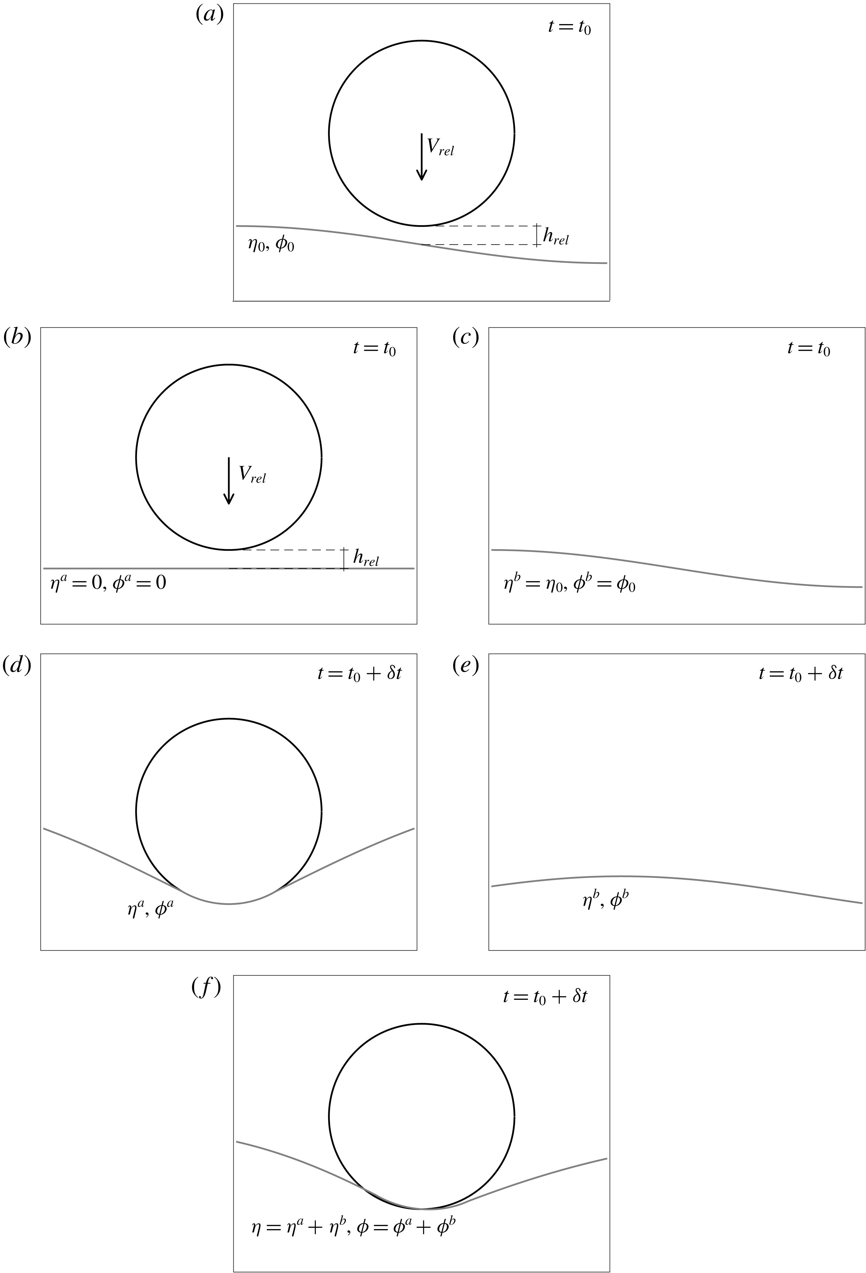
Schematics of the decomposition of the impact of a walking droplet problem into two simpler calculations. Panel (a) shows the initial conditions given by an imminent droplet impact, (b) and (c) show the initial conditions for each of the separate problems, (d) and (e) respectively show the evolution of (b) and (c), and (f) shows how the results (d) and (e) are combined. The sub-index rel indicates magnitudes measured in relation to the point of the free surface that is directly below the south pole of the sphere.

In summary, we model the wave field of a walking droplet by superposing translations of axisymmetric wave fields due to droplet impacts. When the droplet is in flight, we calculate the free-surface evolution by solving the linear equations (2.14) and (2.15), with $\unicode[STIX]{x1D705}=\unicode[STIX]{x1D6E5}_{H}$ , and the droplet height from (2.19); all subject to $p_{s}(\boldsymbol{x},t)=0$ . When an impact is about to happen, we separate the problem into two (see figure 2). We define problem $a$ as the axisymmetric impact of a droplet onto a bath, with the initial conditions $\unicode[STIX]{x1D702}^{a}(\boldsymbol{x},t_{0})=0$ and $\unicode[STIX]{x1D719}^{a}(\boldsymbol{x},t_{0})=0$ , and the position and velocity of the droplet being such that the relative height and vertical velocity with respect to the surface point exactly below the south pole are the same as in the physical problem (figures 2 b and 2 d). For this problem, we preserve the full curvature $\unicode[STIX]{x1D705}$ within $A(t)$ , as done in Galeano-Rios et al. (Reference Galeano-Rios, Milewski and Vanden-Broeck2017). We solve the axisymmetric problem $a$ until the droplet is once again airborne. In parallel, we define problem $b$ in which we find waves $\unicode[STIX]{x1D702}^{b}$ and $\unicode[STIX]{x1D719}^{b}$ with initial conditions $\unicode[STIX]{x1D702}^{b}(\boldsymbol{x},t_{0})=\unicode[STIX]{x1D702}(\boldsymbol{x},t_{0})$ and $\unicode[STIX]{x1D719}^{b}(\boldsymbol{x},t_{0})=\unicode[STIX]{x1D719}(\boldsymbol{x},t_{0})$ , but without the pressure induced by the droplet, which is to say we ignore the forcing of the ongoing droplet contact as we solve the wave field (figures 2 c and 2 e). The temporally dependent nature of gravity is preserved in both problems. We then superpose the axisymmetric solution of the droplet impact on the unforced surface waves at the predicted location of the droplet $\boldsymbol{X}(t)$ . Once the droplet is again in flight, we carry on solving a single problem, namely that resulting from the superposition.

We note that the vertical droplet motion obtained from the impact on the flat free surface is treated as an approximation to the motion of the actual droplet relative to the point on the fluid surface that is directly under the south pole of the droplet. That is to say, the height and velocities of the droplet as obtained from the impact of a flat interface will be added to the height and velocity of the fluid surface at the $\boldsymbol{X}(t)$ location in order to obtain the prediction for the height of the droplet for $t\in [t_{0},t_{l}]$ . We highlight that this superposition does not result in a perfect match of the surfaces (see figure 2 f); however, it still yields an exact match between the south pole of the droplet and the corresponding point of the free surface. The mismatch between the sphere and the free surface of the bath is of the order of the wave gradient in problem $b$ , i.e. $\unicode[STIX]{x1D716}/\unicode[STIX]{x1D706}_{F}=O(10^{-3})$ , multiplied by the radius of the typical pressed area ( ${\leqslant}0.5R_{o}$ ). Therefore, the typical mismatch is of $O(10^{-3})$ when expressed as a fraction of the droplet radius.

2.4 Horizontal dynamics

We derive equations for the horizontal motion of the sphere on the basis of the approximations introduced in § 2.3. For impacts, we arrive at a model that includes the horizontal components of the pressure forces that were previously discussed in § 2.2.2, as well as a drag force due to a simplified model of viscous forces in the intervening air layer similar to the one presented in Couder et al. (Reference Couder, Fort, Gautier and Boudaoud2005a ) and Protière, Boudaoud & Couder (Reference Protière, Boudaoud and Couder2006). The main advantage of the derivation presented in what follows is that we are able to include the effect of changes in pressed area over each contact of the droplet.

The horizontal motion of the droplet, expressed in dimensionless variables, is governed by

(2.46) $$\begin{eqnarray}\displaystyle \boldsymbol{X}_{tt} & = & \displaystyle {\displaystyle \frac{1}{Ma}}\left(\int _{A(t)}{\displaystyle \frac{-p_{s}\unicode[STIX]{x1D735}\unicode[STIX]{x1D702}}{\sqrt{1+|\unicode[STIX]{x1D735}\unicode[STIX]{x1D702}|^{2}}\,}}\,\text{d}A+\int _{S(t)}(\unicode[STIX]{x1D64F}_{air}\boldsymbol{\cdot }\hat{\boldsymbol{n}})_{H}\,\text{d}S\right.\nonumber\\ \displaystyle & & \displaystyle \left.+\,\int _{S^{2}\setminus S(t)}(-p_{air}\hat{\boldsymbol{n}}+\unicode[STIX]{x1D64F}_{air}\boldsymbol{\cdot }\hat{\boldsymbol{n}})_{H}\,\text{d}S\right),\end{eqnarray}$$

where $\unicode[STIX]{x1D64F}_{air}$ is the deviatoric part of the stress tensor for the air flow, $\hat{\boldsymbol{n}}$ is the outward-pointing unit normal to the sphere, $p_{air}$ is the air pressure, the sub-index $H$ indicates the projection onto the $xy$ plane, $S^{2}$ is the surface of the whole sphere, and we recall that $A(t)$ is the horizontal projection of $S(t)$ , the portion of the sphere’s surface that is in contact with the free surface of the bath. The first term in parentheses on the right-hand side of (2.46) corresponds to horizontal forces due to pressure between the two free surfaces; the second corresponds to the horizontal component of the viscous effects of the flow of air in the intervening layer; and the third term accounts for the contribution of horizontal forces due to the air, outside of the pressed area.

Given the scaling considerations discussed in § 2.3, the leading-order term for the pressure forces due to impact yields

(2.47) $$\begin{eqnarray}\displaystyle -{\displaystyle \frac{1}{Ma}}\int _{A(t)}p_{s}{\displaystyle \frac{\unicode[STIX]{x1D735}\unicode[STIX]{x1D702}}{\sqrt{1+|\unicode[STIX]{x1D735}\unicode[STIX]{x1D702}|^{2}}\,}}\,\text{d}A\approx -\unicode[STIX]{x1D735}\unicode[STIX]{x1D702}^{b}|_{(\boldsymbol{X}(t),t)}{\displaystyle \frac{1}{Ma}}\int _{A^{a}(t)}p_{s}^{a}\,\text{d}A, & & \displaystyle\end{eqnarray}$$

where we have also used the assumption that, since surface waves are long when compared to the droplet diameter, the local average of the gradient is approximately equal to $\unicode[STIX]{x1D735}\unicode[STIX]{x1D702}^{b}(\boldsymbol{X}(t),t)$ .

Since we are not simulating the air flow, we approximate the effect of the deviatoric stresses within the pressed area by

(2.48) $$\begin{eqnarray}\displaystyle {\displaystyle \frac{1}{Ma}}\int _{A(t)}(\unicode[STIX]{x1D64F}_{air}\boldsymbol{\cdot }\hat{\boldsymbol{n}})_{H}\sqrt{1+|\unicode[STIX]{x1D735}\unicode[STIX]{x1D702}|^{2}}\,\text{d}A\approx -{\displaystyle \frac{E(t)T_{F}}{m_{s}}}\boldsymbol{X}_{t}, & & \displaystyle\end{eqnarray}$$

with $E(t)$ being a skidding friction coefficient whose form we discuss below. The third term is approximated using Stokes’ drag, assuming the pressed area is a relatively small fraction of the surface area of the sphere, hence

(2.49) $$\begin{eqnarray}\displaystyle {\displaystyle \frac{1}{Ma}}\int _{S^{2}\setminus S(t)}(-p_{air}\hat{\boldsymbol{n}}+\unicode[STIX]{x1D64F}_{air}\boldsymbol{\cdot }\hat{\boldsymbol{n}})_{H}\,\text{d}S\approx So\,\boldsymbol{X}_{t}, & & \displaystyle\end{eqnarray}$$

with $So$ as in (2.18). We thus have

(2.50) $$\begin{eqnarray}\displaystyle \boldsymbol{X}_{tt}=-D(t)\boldsymbol{X}_{t}-\unicode[STIX]{x1D735}\unicode[STIX]{x1D702}^{b}|_{(\boldsymbol{X}(t),t)}{\displaystyle \frac{1}{Ma}}\int _{A^{a}(t)}p_{s}^{a}\,\text{d}A, & & \displaystyle\end{eqnarray}$$

where $D(t)=So+E(t)/(f_{F}m)$ . We note that, during impacts, the term $So$ (due to Stokes’ drag) is negligible.

2.4.1 Skidding friction

Realistic modelling of skidding friction due to the air flow within the lubrication layer requires methods that can solve a free-boundary lubrication theory problem on a curved, non-symmetric geometry that deforms, and whose deformation is coupled to droplet and wave motion. Moreover, it is the non-symmetric part of the solution to this problem that must be responsible for drag in walking droplets. Given the complexity of this problem, prior works have introduced different simplifications to address this effect; for instance, Moláček & Bush (Reference Moláček and Bush2013b ) introduced a scaling argument based on the assumption of a constant pressed area and experimental observations of the horizontal coefficient of restitution in single-droplet impacts on a flat interface.

We recall that our model yields a time-dependent pressed area approximation as part of the solution to the axisymmetric problem $a$ . This allows for the construction of the first skidding friction model that accounts for the effects of the changes in the pressed area during impacts. We thus revisit skidding friction modelling and we are able to derive a working approximation which yields slightly improved predictions (in terms of comparison to experiments) compared to the existing methods and also offers an explanation as to why two competing approaches used in the past by other groups can be seen as expressions of the same effect when we account for changes in the pressed area over an impact.

Assuming the pressed area $A(t)$ is small enough that the part of the sphere in contact with the free surface is almost flat, viscous friction forces in the thin air layer would be approximately given, in dimensional variables, by

(2.51) $$\begin{eqnarray}\displaystyle F_{D}=-\unicode[STIX]{x1D707}_{air}|A(t)|\,\overline{\unicode[STIX]{x2202}_{z}\boldsymbol{u}_{H}|_{(z=\unicode[STIX]{x1D702})}}, & & \displaystyle\end{eqnarray}$$

where $\unicode[STIX]{x1D707}_{air}$ is the dynamic viscosity of air, $|A(t)|$ is the surface area of $A(t)$ , $\boldsymbol{u}_{H}$ is the horizontal velocity of the air, and the bar indicates the mean in the contact area. The expression under the bar should scale as $\boldsymbol{X}_{t}/e$ , where $e$ is the width of the air layer, which we assume does not change substantially during the contact time. We thus make the approximation

(2.52) $$\begin{eqnarray}\displaystyle F_{D}=-\bar{k}\unicode[STIX]{x1D707}_{air}|A(t)|{\displaystyle \frac{\boldsymbol{X}_{t}}{e}}\approx -k\unicode[STIX]{x1D707}_{air}|A^{a}(t)|{\displaystyle \frac{\boldsymbol{X}_{t}}{R_{o}}}, & & \displaystyle\end{eqnarray}$$

where $\bar{k}$ is a scaling factor for the vertical derivative of the horizontal velocity which we absorb into $k=\bar{k}R_{o}/e$ , a drag parameter. Moreover, we approximate the pressed area $A(t)$ by the disc $A^{a}(t)$ . We note that for a typical droplet radius ( $R_{o}\approx 0.4~\text{mm}$ ) and for the typical air layer width ( $e\approx 2~\unicode[STIX]{x03BC}\text{m}$ ) as predicted in Protière et al. (Reference Protière, Boudaoud and Couder2006), we obtain $R_{o}/e\approx 200$ , which suggests that the values of the dimensionless coefficient $k$ should be of the order of $O(100\bar{k})$ .

In principle, $k$ could be different for each value of driving acceleration or even impact velocity and impact phase, as well as other factors; however, in the present work, we will treat $k$ as constant with respect to those variables. Consequently, in (2.48), we estimate

(2.53) $$\begin{eqnarray}\displaystyle E(t)=k{\displaystyle \frac{\unicode[STIX]{x1D707}_{air}}{R_{o}}}|A^{a}(t)|, & & \displaystyle\end{eqnarray}$$

which in (2.50), in dimensionless variables, yields

(2.54) $$\begin{eqnarray}\displaystyle \boldsymbol{X}_{tt}=-{\displaystyle \frac{3Da}{4Ra}}\left(6+k{\displaystyle \frac{|A^{a}(t)|}{\unicode[STIX]{x03C0}R_{o}^{2}}}\right)\boldsymbol{X}_{t}-\unicode[STIX]{x1D735}\unicode[STIX]{x1D702}^{b}|_{(\boldsymbol{X},t)}{\displaystyle \frac{1}{Ma}}\int _{A^{a}(t)}p_{s}^{a}\,\text{d}A, & & \displaystyle\end{eqnarray}$$

where $Ra=R_{o}^{2}\,f_{F}/\unicode[STIX]{x1D708}_{air}$ and $Da=\unicode[STIX]{x1D70C}_{air}/\unicode[STIX]{x1D70C}$ , with $\unicode[STIX]{x1D708}_{air}$ and $\unicode[STIX]{x1D70C}_{air}$ being the kinematic viscosity and the density of air, respectively. We note that the only undetermined parameter in this equation is $k$ , whose value we set as described later in the text. We anticipate, however, that the term $k(|A^{a}(t)|/\unicode[STIX]{x03C0}R_{o}^{2})$ will dominate the drag effect, in accordance with the relatively minor effect that air drag during flight has been shown to have; for instance, using the model of Milewski et al. (Reference Milewski, Galeano-Rios, Nachbin and Bush2015), we see nearly unchanging walking speeds with or without Stokes’ drag.

3.1 Simulations

Figure 3.

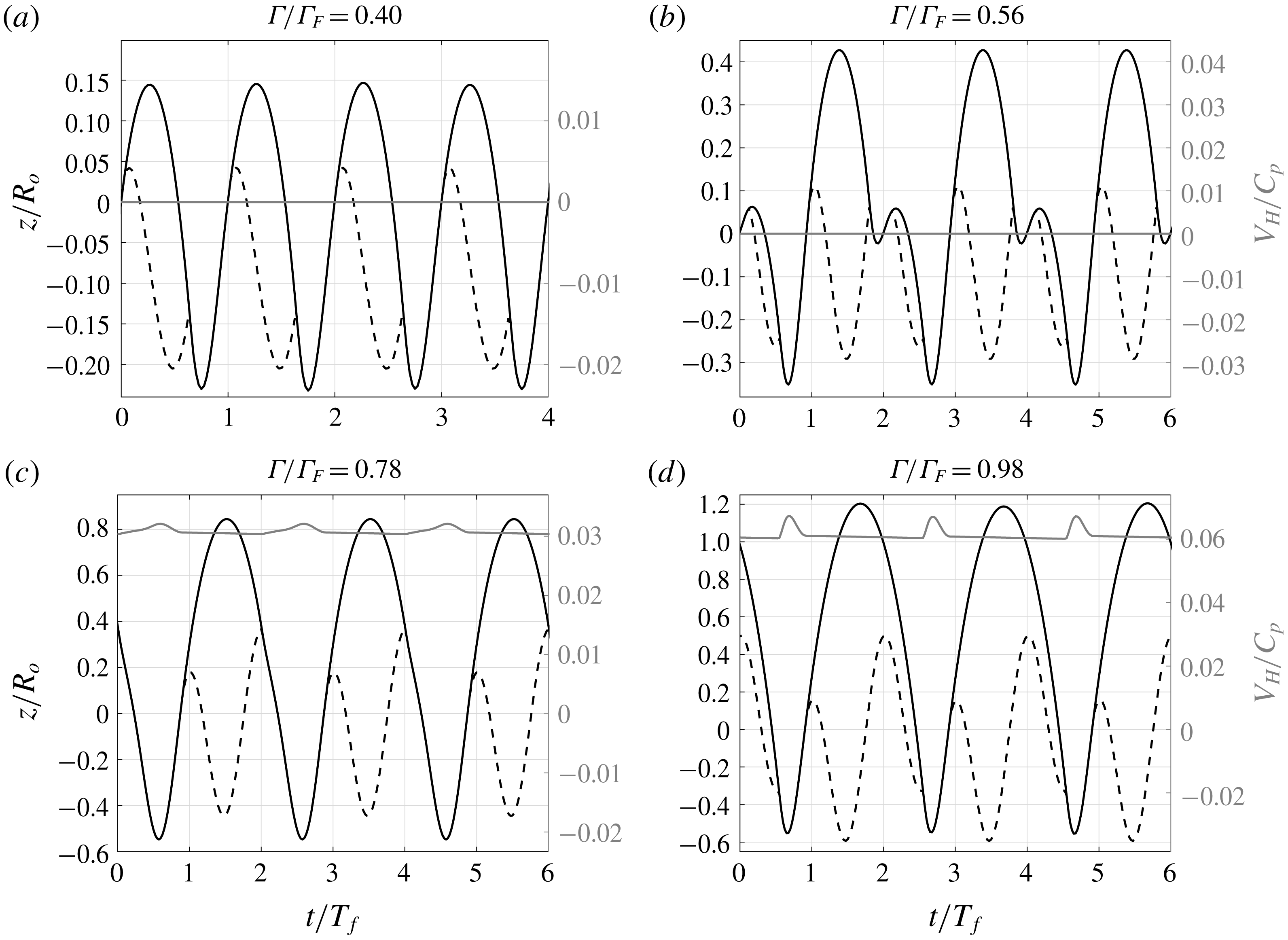
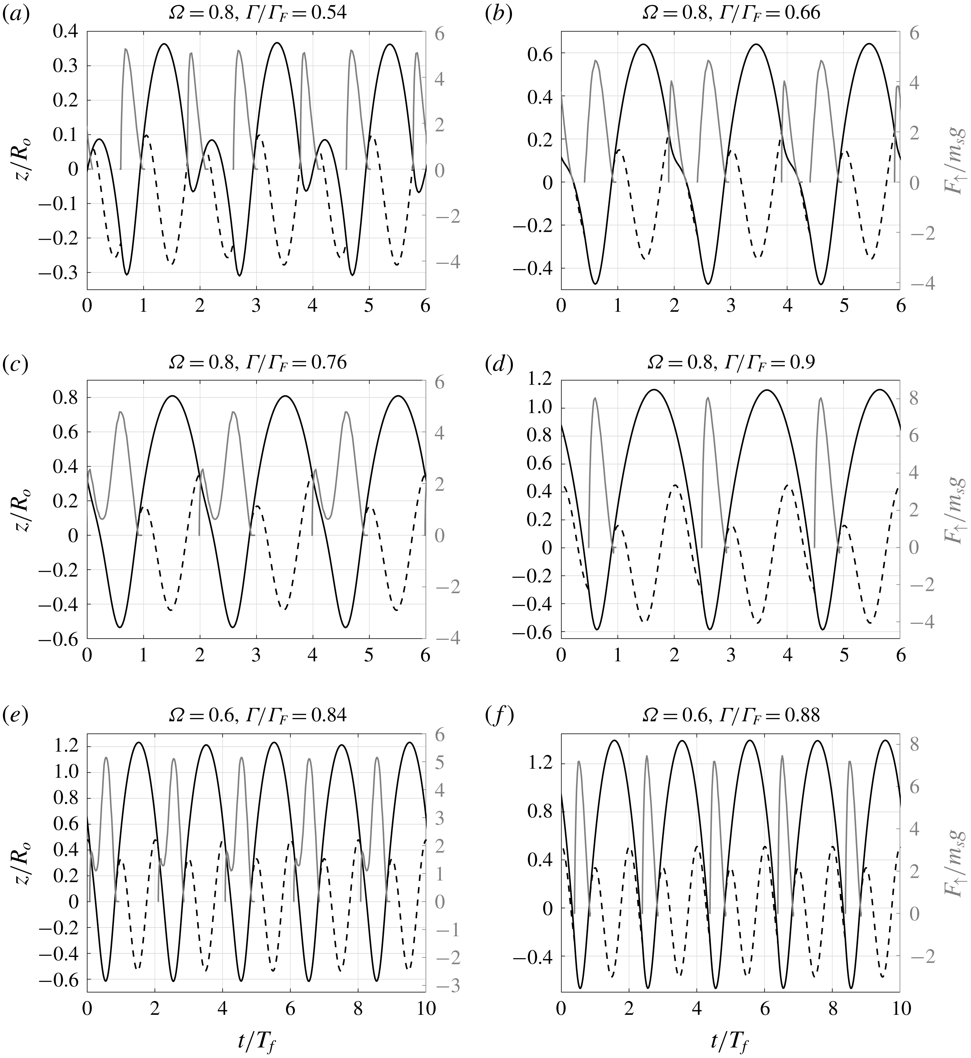
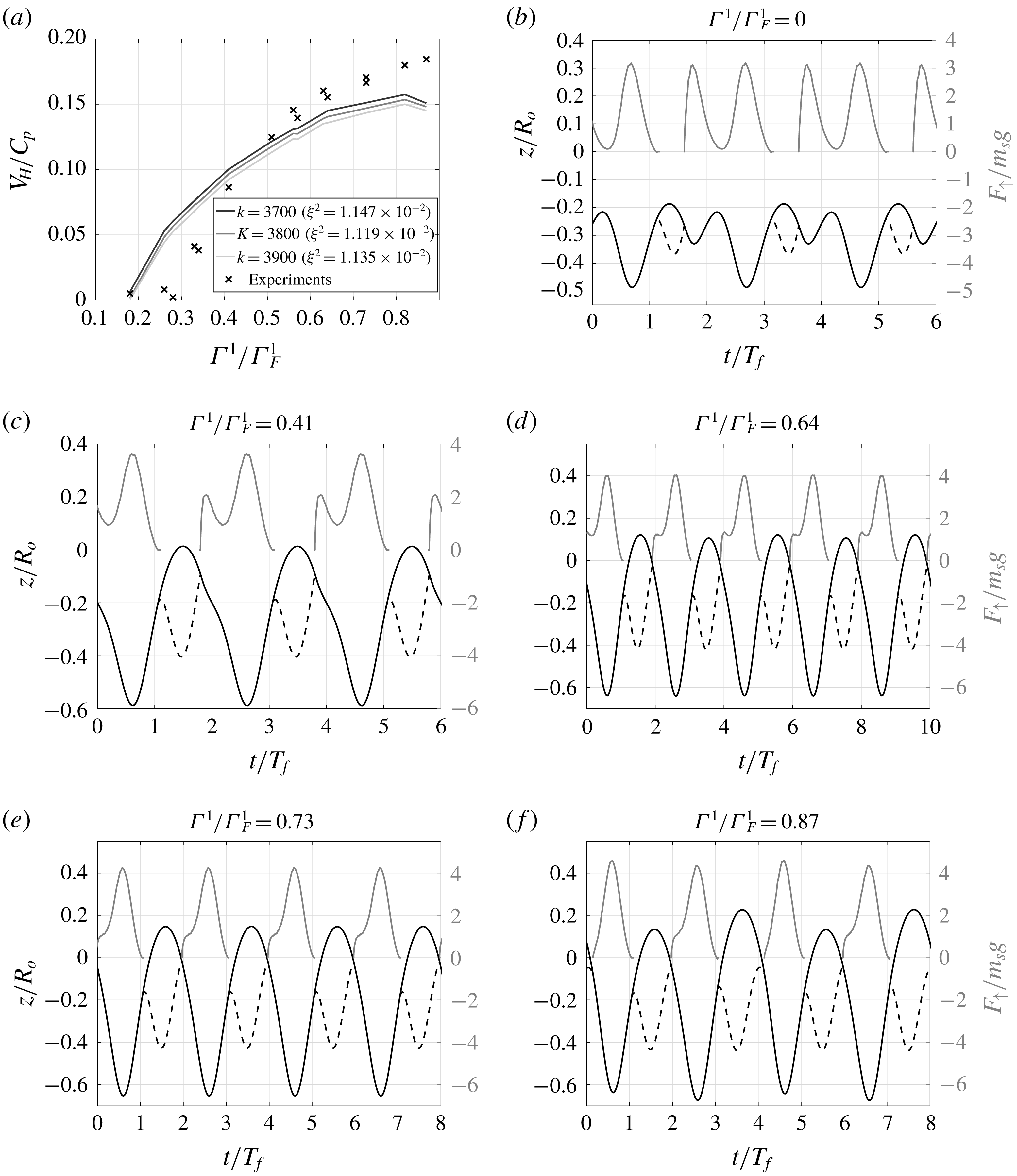
Simulation results for droplets walking at different driving accelerations ( $\unicode[STIX]{x1D6E4}$ ). Solid black lines show the trajectory of the south pole of the droplet and dashed lines correspond to the point of the free surface just under the south pole. Grey lines show the horizontal speed of the droplets. Here $C_{p}$ is the phase velocity of the Faraday waves ( $C_{p}=19.88~\text{cm}~\text{s}^{-1}$ ), and $T_{f}$ is the forcing period. All panels correspond to a droplet of radius $R_{o}=0.38~\text{mm}$ , i.e. vibration number $\unicode[STIX]{x1D6FA}=0.8$ ( $\unicode[STIX]{x1D6FA}=\unicode[STIX]{x1D714}_{o}\sqrt{\unicode[STIX]{x1D70C}R_{o}^{3}/\unicode[STIX]{x1D70E}}$ ) and drag parameter $k=3100$ . Panels (a–c) and (d) correspond to modes $(1,1)$ , $(2,2)$ , $(2,1)^{1}$ and $(2,1)^{2}$ , respectively.

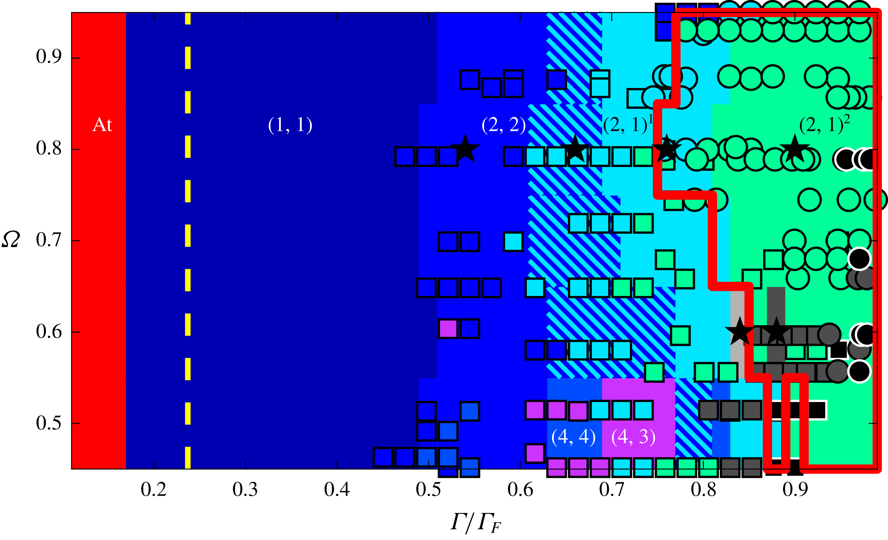
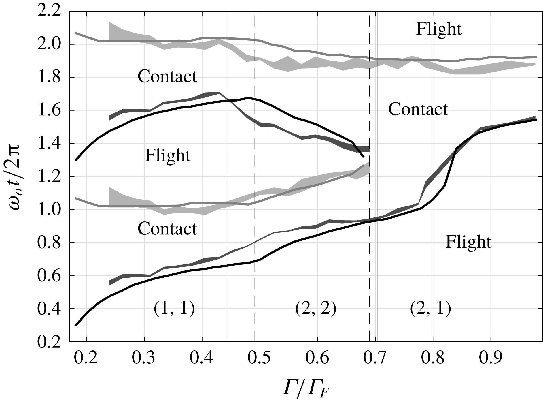
Simulations are initiated by imparting the droplet with a horizontal velocity of $0.1C_{p}$ and with a downward vertical velocity that is in the typical range for walking droplets; all while the droplet is slightly above the surface. Droplets will then settle onto a steady walking speed or come to a halt, if the system parameters do not allow steady walking. We are able to identify the known bouncing modes which we describe with the ordered pairs $(m,n)$ , following Gilet & Bush (Reference Gilet and Bush2009) and Moláček & Bush (Reference Moláček and Bush2013a ), in which $m$ stands for the number of forcing periods contained in a complete period of vertical motion, and $n$ corresponds to the number of contacts that take place during $m$ forcing periods. These different modes can be identified in figure 3, in which droplet contacts correspond to the time intervals over which the south pole coincides with the free surface. We are also able to distinguish variants within the same $(m,n)$ mode, such as the $(2,1)^{1}$ and $(2,1)^{2}$ (see figures 3 c and 3 d). We discuss the distinction of these modes in greater detail later in the text.

Figure 4.

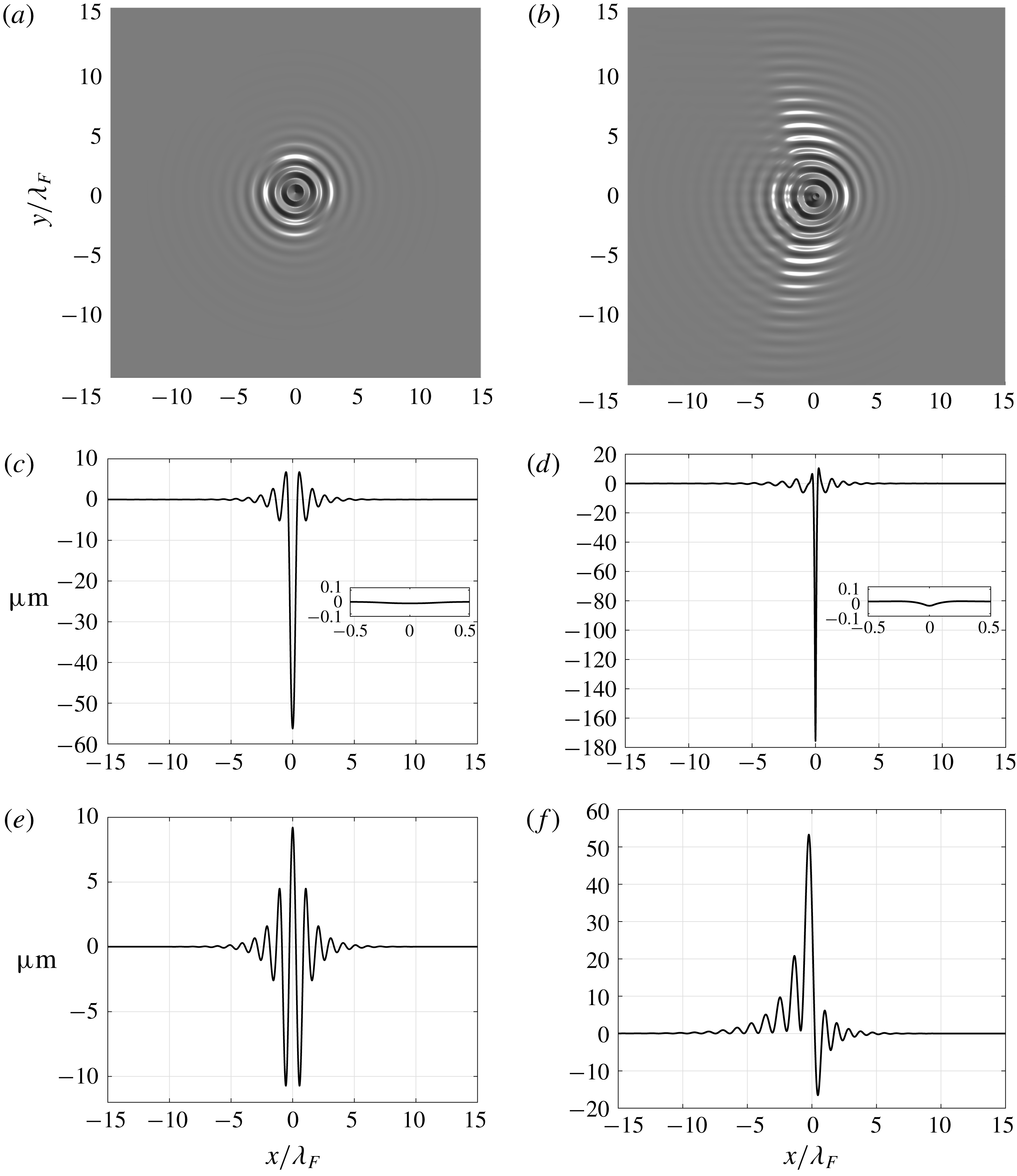
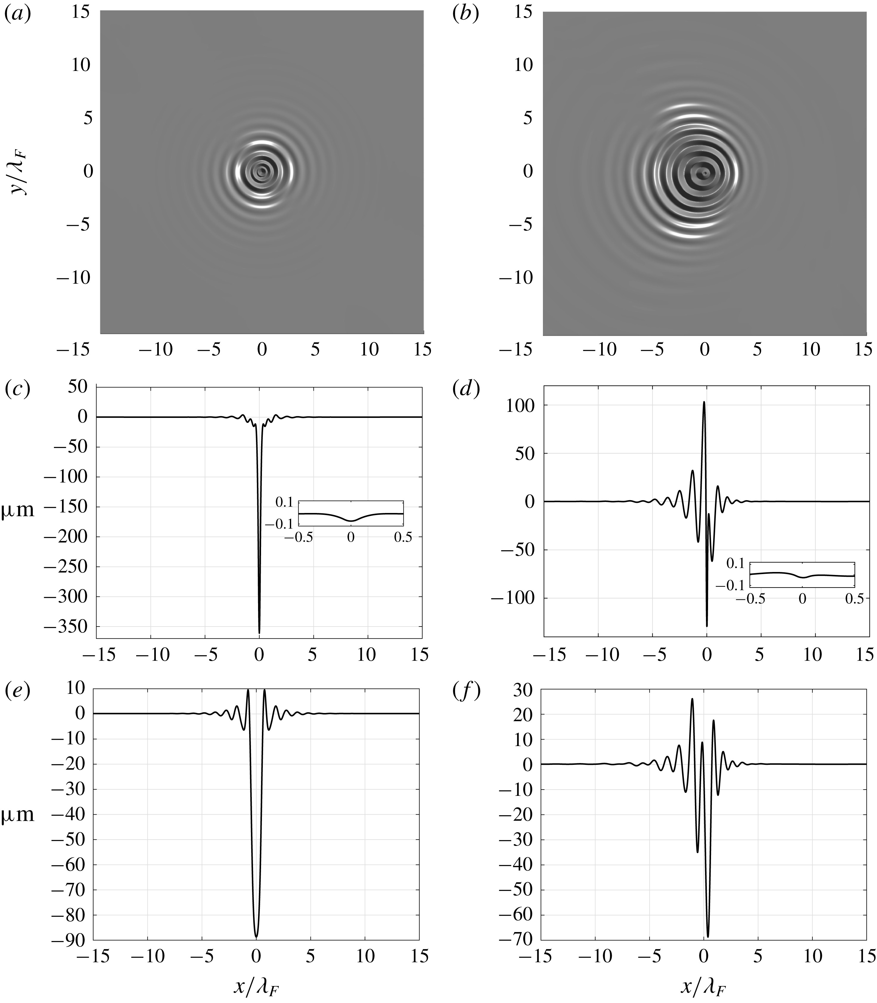
Wave field simulations for vibration number $\unicode[STIX]{x1D6FA}=0.8$ and drag parameter $k=3100$ . (a) Bouncer at $\unicode[STIX]{x1D6E4}/\unicode[STIX]{x1D6E4}_{F}=0.74$ , with (c) its cross-section at $y=0$ . (b) Walker moving to the right at $\unicode[STIX]{x1D6E4}/\unicode[STIX]{x1D6E4}_{F}=0.98$ , with (d) its section along the direction of walking. The wave field in panels (a–c) and (d) is sampled at the time of maximum absolute surface deflection and with $\boldsymbol{X}(t)=(0,0)$ . The inset plots in panels (c) and (d) show a close-up of the wave field at the impact location using the same vertical and horizontal scale (units of $\unicode[STIX]{x1D706}_{F}$ ). The cross-sections in panels (e) and (f) are analogous to those in (c) and (d), respectively; though in (e) and (f) the section is obtained just before a droplet impact. Animations of the wave field and droplet motion for these two simulations are included as supplementary movies available at https://doi.org/10.1017/jfm.2019.409. We note that the panels do not show the totality of the computational domain.

Figure 4 shows the simulation of the wave fields of a bouncer and a walker, which display the typical features reported in Eddi et al. (Reference Eddi, Sultan, Moukhtar, Fort, Rossi and Couder2011). We highlight that the vertical scale in figure 4(c–f) is greatly exaggerated in order to provide a quantitative comparison of the scales of the unforced waves and the impact dimple. This might create the illusion of a non-smooth interface. The inset plots in figure 4(c) and (d) (for which we use the same scale in $x$ and $z$ ) show that the free surface is in fact very smooth. Animations of the simulations presented in figure 4 are provided as supplementary movies; these also clearly portray the surface smoothness.

We run simulations of walking droplets in the parameter regimes investigated experimentally by previous works (Moláček & Bush Reference Moláček and Bush2013b ; Wind-Willassen et al. Reference Wind-Willassen, Moláek, Harris and Bush2013; Pucci et al. Reference Pucci, Sáenz, Faria and Bush2016) with the experimental set-up of $20~\text{cSt}$ and $80~\text{Hz}$ (see appendix A) for different values of the vibration number $\unicode[STIX]{x1D6FA}=\unicode[STIX]{x1D714}_{o}\sqrt{\unicode[STIX]{x1D70C}R_{o}^{3}/\unicode[STIX]{x1D70E}}$ (as defined in Dorbolo et al. (Reference Dorbolo, Terwagne, Vandewalle and Gilet2008)); we then compare their experimental reports to our simulation results for different values of the skidding friction parameter $k$ . We use the comparison to define an adequate value of $k$ for each $\unicode[STIX]{x1D6FA}$ and complete our skidding friction model. We note that, since all other parameters involved in the definition of $\unicode[STIX]{x1D6FA}$ are fixed for this study, $\unicode[STIX]{x1D6FA}$ can be simply considered as a proxy for the droplet radius.

3.1.1 Optimal values of $k$

Protière et al. (Reference Protière, Boudaoud and Couder2006) proposed a skidding friction model in which viscous effects yield a force that is proportional to droplet speed, where the proportionality constants were estimated on the basis of typical sizes for the contact area and air layer width. Moláček & Bush (Reference Moláček and Bush2013b ) presented a different skidding friction model in which the horizontal drag force due to the motion of the droplet as it slides on the surface is considered to be proportional to the vertical force exerted on the droplet, and to the droplet speed. They arrived at this form for the drag by means of experimental measurements of the horizontal coefficient of restitution of droplets impacting a bath at different angles. They go on to fit the resulting data of tangential coefficient of restitution as a function of the Weber number and interpret their findings as implying that the dominant effect for horizontal drag is momentum transference to the fluid bath. Moreover, they assume throughout their work that the pressed area is roughly constant.

Our present approach is similar to that of Protière et al. (Reference Protière, Boudaoud and Couder2006); however, we are able to consider the change in contact area during each impact. We obtain, as shown in (2.52), a friction model that is proportional to the instantaneous value of the contact area and to the droplet’s velocity. Nevertheless, in Galeano-Rios et al. (Reference Galeano-Rios, Milewski and Vanden-Broeck2017) it was shown that the pressed area and the vertical force are roughly proportional; therefore, a model that accounts for pressed area variations will produce a skidding friction term that is approximately proportional to forces and droplet speeds. Thus, when we account for the effects of the varying pressed area, we can reinterpret the findings of Moláček & Bush (Reference Moláček and Bush2013b ) as not being incompatible with those of Protière et al. (Reference Protière, Boudaoud and Couder2006). In particular, we can justify the form of the friction term given in Moláček & Bush (Reference Moláček and Bush2013b ) whilst still considering viscous effects as the main drivers of the resistance to motion during contact.

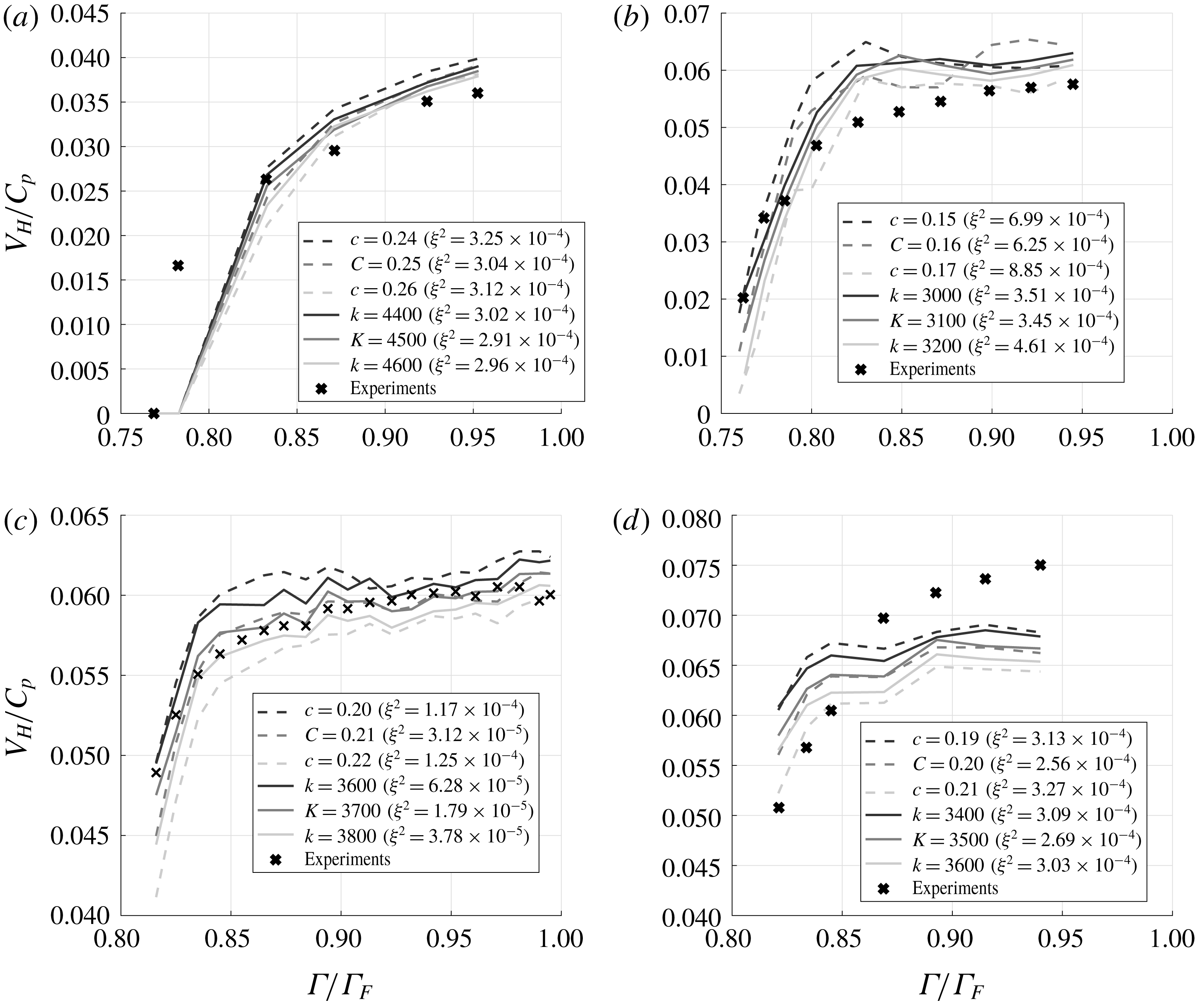
To find the optimal value $K$ of the proportionality constant $k$ for each droplet size (i.e. $\unicode[STIX]{x1D6FA}$ ) for which the walking speed was reported at different driving accelerations in the experimental works, we test a sequence of values of $k$ . For each tested $k$ we find the differences $\unicode[STIX]{x1D709}_{i}$ between the experimental report for horizontal speed $u_{i}^{e}$ and the average horizontal speed as calculated from the simulations $u_{i}^{s}$ , where the $i$ th experimental point corresponds to a given value of $\unicode[STIX]{x1D6E4}_{i}/\unicode[STIX]{x1D6E4}_{F}$ (see figure 5). We thus define the total squared error for each attempted value of the drag parameter $k$ as

(3.24) $$\begin{eqnarray}\displaystyle \unicode[STIX]{x1D709}^{2}(k,\unicode[STIX]{x1D6FA})=\mathop{\sum }_{i=1}^{n}\unicode[STIX]{x1D709}_{i}^{2}(k,\unicode[STIX]{x1D6FA},\unicode[STIX]{x1D6E4}_{i}/\unicode[STIX]{x1D6E4}_{F})=\mathop{\sum }_{i=1}^{n}(u_{i}^{e}-u_{i}^{s})^{2}(k,\unicode[STIX]{x1D6FA},\unicode[STIX]{x1D6E4}_{i}/\unicode[STIX]{x1D6E4}_{F}), & & \displaystyle\end{eqnarray}$$

and we define

(3.25) $$\begin{eqnarray}\displaystyle K(\unicode[STIX]{x1D6FA})=\text{argmin}\,\unicode[STIX]{x1D709}^{2}(\cdot ,\unicode[STIX]{x1D6FA}). & & \displaystyle\end{eqnarray}$$

Figure 5.

Walker speed as a function of $\unicode[STIX]{x1D6E4}$ for different values of the drag parameter $k$ , normalised by Faraday wave phase velocity ( $C_{p}=19~\text{cm}~\text{s}^{-1}$ in experiments, and $C_{p}=19.88~\text{cm}~\text{s}^{-1}$ in simulations): (a) $\unicode[STIX]{x1D6FA}=0.7$ , (b) $\unicode[STIX]{x1D6FA}=0.8$ , (c) $\unicode[STIX]{x1D6FA}=0.83$ , (d) $\unicode[STIX]{x1D6FA}=0.86$ . Dashed lines correspond to the skidding friction model presented in Moláček & Bush (Reference Moláček and Bush2013b ), solid lines correspond to the skidding friction model developed in the present work. Experimental data for (a), (b) and (d) were obtained from Moláček & Bush (Reference Moláček and Bush2013b ), and data for (c) from Pucci et al. (Reference Pucci, Sáenz, Faria and Bush2016)

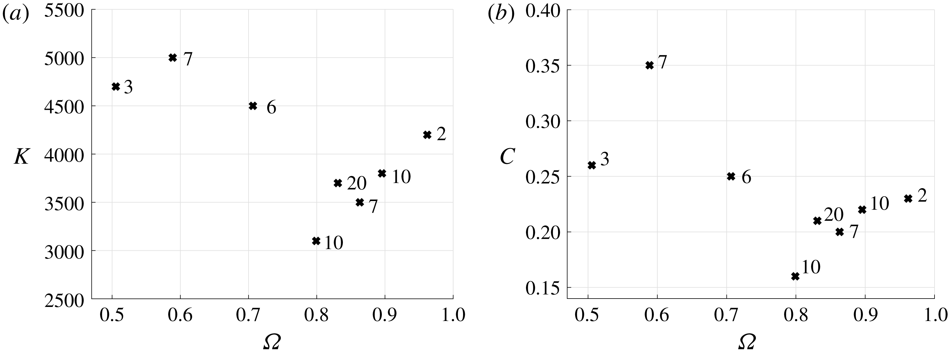
The values of $K(\unicode[STIX]{x1D6FA})$ are identified up to two significant figures and are reported in figure 5. Figure 6(a) shows the distribution of $K(\unicode[STIX]{x1D6FA})$ . We perform an entirely analogous calculation, using the friction model presented in Moláček & Bush (Reference Moláček and Bush2013b ), in which $F_{D}=-c\sqrt{\unicode[STIX]{x1D70C}R_{o}/\unicode[STIX]{x1D70E}}\,F(t)\boldsymbol{X}_{t}$ , and we obtain a similar distribution of values for the corresponding optimal proportionality constant $C(\unicode[STIX]{x1D6FA})$ . The respective walking speed predictions are reported in dashed lines in figure 5 and the distribution of $C(\unicode[STIX]{x1D6FA})$ is presented in figure 6(b). In practice, the value of $C$ used in different models ranges from $0.1$ to $0.35$ , as can be seen in the literature (Moláček & Bush Reference Moláček and Bush2013b ; Oza et al. Reference Oza, Rosales and Bush2013; Milewski et al. Reference Milewski, Galeano-Rios, Nachbin and Bush2015; Durey & Milewski Reference Durey and Milewski2017).

The agreement between theory and experiment shown in figure 5 is overall good, especially when considering the simplifications introduced; however, there clearly is room for improvement. The choice to stop at two significant figures in determining $K$ is based on the fact that the two neighbouring values at that precision provide an obvious bound to how much the predictions can be improved by a more precise value of $K$ , which indicate that no qualitative agreement is likely to be gained. A more complete understanding of the air flow in the intervening air layer would enable the production of better reduced models, as it would allow for a realistic treatment of the dependence of the $\bar{k}$ scaling factor on time or pressure distribution, and also of the time-varying air layer width $e$ . As part of our ongoing work, we have posed the problem including a coupled lubrication theory equation which we will attempt to address once we have successfully incorporated droplet deformations.

The skidding friction parameter $k$ is $O(10^{3})$ and $|A^{a}(t)|/(\unicode[STIX]{x03C0}R_{0}^{2})$ (i.e. the fraction of the droplet’s ‘shadow’ that is pressed) is $O(10^{-1})$ . Therefore $k|A^{a}(t)|/(\unicode[STIX]{x03C0}R_{0}^{2})$ is of order $O(10^{2})$ , which is significantly larger than $6$ (the factor that corresponds to Stokes’ drag). This verifies the intuition suggested at the end of § 2.4.1. Moreover, the value of $1/Ma$ (the reciprocal of the dimensionless mass of the droplet) ranges from $425$ (biggest walking droplets) to $1334$ (smallest walking droplets). This is consistent with walking droplet motion being dominated by the forces exerted by the waves onto the droplets, and also with bigger droplets, such as the superwalker considered in § 4.1 (for which $1/Ma=93$ ), being less prone to walking under single-frequency forcing.

Figure 6.

Skidding friction coefficients for the two models here considered. Panel (a) shows $K(\unicode[STIX]{x1D6FA})$ for the proposed model, and panel (b) shows $C(\unicode[STIX]{x1D6FA})$ for the model in Moláček & Bush (Reference Moláček and Bush2013b ). Numbers alongside the markers indicate the number of data points available in the literature for a given droplet size.

The similarity between figures 6(a) and 6(b) is consistent with the finding of the approximate proportionality between vertical force and pressed area reported in Galeano-Rios et al. (Reference Galeano-Rios, Milewski and Vanden-Broeck2017). We note that our proposed skidding friction model produces less total errors ( $\unicode[STIX]{x1D709}^{2}(K(\unicode[STIX]{x1D6FA}),\unicode[STIX]{x1D6FA})$ ) for most values of $\unicode[STIX]{x1D6FA}$ and that the relative deviation with respect to the mean value is smaller for $K$ ( $\unicode[STIX]{x1D70E}_{d}(K)/\bar{K}=0.16$ , $\unicode[STIX]{x1D70E}_{d}(C)/\bar{C}=0.24$ ). In what follows, we use $K(\unicode[STIX]{x1D6FA})$ for each droplet radius.

4.1 Superwalkers: two-frequency shaking

Valani et al. (Reference Valani, Slim and Simula2019) recently reported a new kind of walking droplets. These are relatively large droplets (up to 1.4 mm radius) that always bounce in place when the underlying bath is subject to simple harmonic motion, but walk particularly fast (up to approximately three times the maximum velocity for regular walkers, i.e. $C_{w}/C_{p}\approx 0.15$ ) when the bath is subject to vertical oscillations obtained using the superposition of two sinusoidal signals of different frequencies. More specifically, this was observed to happen when the second frequency added is resonant with the subharmonic Faraday waves. The most relevant predecessor of this work is Sampara & Gilet (Reference Sampara and Gilet2016), who considered a combination of 80 and 64 Hz forcing in a bath of 20 cSt silicone oil, and were thus able to find a series of novel trajectories for the walking droplet system.

Valani et al. (Reference Valani, Slim and Simula2019) drive the oil bath with a vertical acceleration of the form

(4.1) $$\begin{eqnarray}\displaystyle z_{tt}=-g(\unicode[STIX]{x1D6E4}\cos (\unicode[STIX]{x1D714}_{o}t)+\unicode[STIX]{x1D6E4}^{1}\cos ({\textstyle \frac{1}{2}}\unicode[STIX]{x1D714}_{o}t+\unicode[STIX]{x1D703}_{1})), & & \displaystyle\end{eqnarray}$$

and therefore have two extra physical parameters with respect to the regular walking droplet experiment; namely, the subharmonic forcing amplitude, controlled by $\unicode[STIX]{x1D6E4}^{1}$ , and the phase shift between the two frequencies, given by $\unicode[STIX]{x1D703}_{1}$ . Regarding the bath motion, the two main differences between Sampara & Gilet (Reference Sampara and Gilet2016) and Valani et al. (Reference Valani, Slim and Simula2019) are the choice of the second frequency as resonant with the subharmonic Faraday waves and the introduction of the phase shift parameter, which was kept constant and equal to zero in Sampara & Gilet (Reference Sampara and Gilet2016). Moreover, the droplet size considered in Sampara & Gilet (Reference Sampara and Gilet2016) is in the regular walker size range. These differences explain why the superwalkers where not observed in their work.

The changes to the problem formulation, needed to model superwalkers, amount to replacing each instance of the expression

(4.2) $$\begin{eqnarray}\displaystyle {\displaystyle \frac{(1-\unicode[STIX]{x1D6E4}\cos (4\unicode[STIX]{x03C0}t))}{Fr}} & & \displaystyle\end{eqnarray}$$

in (3.2), (3.3), (3.10), (3.11) and (3.17) by

(4.3) $$\begin{eqnarray}\displaystyle {\displaystyle \frac{(1-\unicode[STIX]{x1D6E4}\cos (4\unicode[STIX]{x03C0}t)-\unicode[STIX]{x1D6E4}^{1}\cos (2\unicode[STIX]{x03C0}t+\unicode[STIX]{x1D703}_{1}))}{Fr}}, & & \displaystyle\end{eqnarray}$$

and selecting an appropriate value for the skidding friction constant $k$ . Another minor modification to simulate superwalkers is the use of a larger axisymmetric impact domain, i.e. a domain of radius $4\unicode[STIX]{x1D706}_{F}$ (twice the diameter of the one used for regular walkers). This choice was made to guarantee that waves triggered by large droplets, which sometimes produce contacts that are twice as long as those of walkers, do not reach the boundary of the axisymmetric domain before the impact is over.

We highlight that superwalking droplets undergo a non-negligible amount of deformation. In particular, one can see that the droplet’s Bond ( $Bo_{d}=\unicode[STIX]{x1D70C}gR^{2}/\unicode[STIX]{x1D70E}$ ) and Weber ( $We_{d}=\unicode[STIX]{x1D70C}RV_{rel}^{2}/\unicode[STIX]{x1D70E}$ ) numbers are larger that those for regular walkers, which indicates that deformations induced by gravity and inertia will be more prevalent. Typical physical parameters for a walking droplet yield $Bo_{d}=0.0671$ and $We_{d}=0.195$ , whereas for the superwalkers considered here $Bo_{d}=0.91$ and $We_{d}=0.261$ . Moreover, the ratio of walking speed $C_{w}$ to the relative vertical speed before impact $U_{z}$ is $C_{w}/U_{z}\approx 0.6$ . We therefore consider that the main motivation for the present section is to demonstrate the surprising extent to which a model based on a non-deforming droplet can capture (super)walking droplet phenomena.

Figure 11.

Superwalkers at $\unicode[STIX]{x1D6FA}=1.91$ ( $R_{o}=0.68~\text{mm}$ ),  $\unicode[STIX]{x1D6E4}/\unicode[STIX]{x1D6E4}_{F}=0.71$ and $\unicode[STIX]{x1D703}_{1}=8\unicode[STIX]{x03C0}/9$ . (a) Average velocity of superwalkers for different values of the drag parameter $k$ , normalised by the phase velocity of the Faraday wave of frequency 40 Hz ( $C_{p}=19~\text{cm}~\text{s}^{-1}$ in experiments, and $C_{p}=19.88~\text{cm}~\text{s}^{-1}$ in the simulations). Vertical trajectories of the south pole (solid black lines) and of the free-surface point just underneath (dashed lines) are shown, together with vertical forces $F_{\uparrow }$ on droplets for different driving accelerations $\unicode[STIX]{x1D6E4}^{1}$ . Panels (b–f) show a droplet bouncing at single frequency forcing in the $(2,1)^{1}$ mode (b), walking in the $(2,1)^{1}$ mode (c), walking in the $(4,2)^{1}$ mode (d), walking in the $(2,1)^{2}$ mode (e), and walking in the $(4,2)^{2}$ mode (f). Experimental data in panel $(a)$ were obtained from Valani, Slim & Simula (Reference Valani, Slim and Simula2018).

In figure 3(a) of Valani et al. (Reference Valani, Slim and Simula2019), it is shown that superwalkers only appear in a window of the $\unicode[STIX]{x1D703}_{1}$ parameter that is centred roughly about $\unicode[STIX]{x1D703}_{1}=7\unicode[STIX]{x03C0}/9$ . Moreover, in figure 2(c) of Valani et al. (Reference Valani, Slim and Simula2018), the walking speed of a superwalker of $R_{o}=0.68~\text{mm}$ for fixed $\unicode[STIX]{x1D6E4}/\unicode[STIX]{x1D6E4}_{F}=0.71$ and $\unicode[STIX]{x1D703}_{1}=8\unicode[STIX]{x03C0}/9$ is reported as a function of $\unicode[STIX]{x1D6E4}^{1}/\unicode[STIX]{x1D6E4}_{F}^{1}$ , with $\unicode[STIX]{x1D6E4}_{F}^{1}$ given by the Faraday threshold for the fluid bath when driven at an angular frequency of $\unicode[STIX]{x1D714}_{o}/2$ . The superwalker phenomenon is reproduced for any value of the drag parameter $k$ in the order of the values chosen for $K(\unicode[STIX]{x1D6FA})$ (figure 6). That is to say, droplets bounce when in the presence of a single frequency and walk faster than typical walkers (up to more than twice as fast as the fastest walkers) when the second frequency is added to the driving. To find the optimal $K(\unicode[STIX]{x1D6FA})$ for $\unicode[STIX]{x1D6FA}(R_{o}=0.68)$ , we test different values of $k$ and find the one that minimises the squared error with respect to the experimental results reported in figure 2(c) of Valani et al. (Reference Valani, Slim and Simula2018).

Figure 11(a) shows the comparison between the experimental report of superwalker velocity (Valani et al. Reference Valani, Slim and Simula2019) and our simulation results for values of $k$ in the vicinity of its optimal value $K(\unicode[STIX]{x1D6FA}=1.91)$ . Figures 11(b–f) show the modes of bouncing displayed and the forces on the droplet due to collisions with the bath. When in the presence of a single-frequency forcing (figure 11 b), $\unicode[STIX]{x1D6E4}_{1}=0$ ; the droplet bounces in place displaying a $(2,1)^{1}$ mode with a particularly long contact. We note that our model shows in fact that the superwalkers are barely lifting off the surface when a single frequency is present. As the second frequency is introduced (figure 11 c–f), the droplet walks even for $\unicode[STIX]{x1D6E4}^{1}/\unicode[STIX]{x1D6E4}_{F}^{1}$ as low as $0.18$ (figures 11 a and 11 b). As in the case of the walkers, the mode of bouncing observed changes with the driving acceleration ( $\unicode[STIX]{x1D6E4}^{1}$ , in this case). In figure 11, we see the superwalkers bifurcation sequence: $(2,1)^{1}\rightarrow (4,2)^{1}\rightarrow (2,1)^{2}\rightarrow (4,2)^{2}$ . It is worth noting that, even though the skidding friction coefficient is of the same order as the one used for regular walkers, the walking speeds we obtain are in line with the superwalker experiments (up to three times the speed of single-frequency walkers).

We note that our model predicts that the superwalkers have a wave field that is qualitatively different from that of single-frequency walkers. As can be seen in figure 12(b), the wave field behind the superwalker does not exhibit, for these parameters, the typical interference pattern reported by Eddi et al. (Reference Eddi, Sultan, Moukhtar, Fort, Rossi and Couder2011), also observable in figure 4(b). Experimental reports from Valani et al. (Reference Valani, Slim and Simula2019) show that the wave field of the superwalkers indeed looks like our predictions. This distinctive wave field is likely due to the fact that we are exciting Faraday waves under two-frequency forcing, which will respond to a Mathieu equation that is different from the one for single-frequency forcing found by Benjamin & Ursell (Reference Benjamin and Ursell1954); see Zhang & Vinals (Reference Zhang and Vinals1997). In particular, the Fourier transform of the wave field contains a higher contribution of wavelengths in the range of the Faraday wavelength for 40 Hz forcing ( $k\approx 7.16~\text{cm}^{-1}$ ). Moreover, the wave field associated with such a large droplet deforms the free surface substantially in the vicinity of the droplet, as can also be seen in figures 11(b–f), even in the absence of a second forcing frequency (figures 11 b and 12 a). We highlight that the inset plots in figures 12 $(c)$ and 12 $(d)$ show that the surface remains smooth at the impact location. This can also be appreciated in the corresponding animation of the simulations results from the cases in figure 12, which are provided as supplementary movies.

Figure 12.

Wave field predictions for $\unicode[STIX]{x1D6FA}=1.91$ , $\unicode[STIX]{x1D6E4}/\unicode[STIX]{x1D6E4}_{F}=0.71$ and $\unicode[STIX]{x1D703}_{1}=8\unicode[STIX]{x03C0}/9$ . (a) Bouncer at $\unicode[STIX]{x1D6E4}^{1}/\unicode[STIX]{x1D6E4}_{F}^{1}=0$ , and (b) superwalker moving to the right at $\unicode[STIX]{x1D6E4}^{1}/\unicode[STIX]{x1D6E4}_{F}^{1}=0.87$ . Panels $(c)$ and $(d)$ show cross-sections of the wave field represented in $(a)$ and $(b)$ , respectively. The wave fields in panels (a–c) and $(d)$ are sampled at the time at which the maximum surface deflection (in absolute value) occurs while the droplet is located at $\boldsymbol{X}(t)=(0,0)$ . Inset plots in panels $(c)$ and $(d)$ show the impact location using the same scale for the vertical and horizontal axes (units of $\unicode[STIX]{x1D706}_{F}$ ). Panels $(e)$ and $(f)$ show the respective analogous cross-sections to $(c)$ and $(d)$ ; though taken just before a droplet impact. Animations of the wave field and droplet motion for these two simulations are included as supplementary movies.

To the best of our knowledge, no other model has captured superwalker phenomena. In particular, we attempted to use the model presented in Milewski et al. (Reference Milewski, Galeano-Rios, Nachbin and Bush2015) and obtained a significant mismatch in the vertical dynamics.

The superwalker phenomenon is one more piece of evidence for the extremely rich dynamics associated with the bouncing droplet system. A more complete treatment of superwalkers requires the consideration of droplet deformation and will be the subject of future work.